Positive-Unlabeled Node Classification
with Structure-aware Graph Learning

Abstract.

Node classification on graphs is an important research problem with many applications. Real-world graph data sets may not be balanced and accurate as assumed by most existing works. A challenging setting is positive-unlabeled (PU) node classification, where labeled nodes are restricted to positive nodes. It has diverse applications, e.g., pandemic prediction or network anomaly detection. Existing works on PU node classification overlook information in the graph structure, which can be critical. In this paper, we propose to better utilize graph structure for PU node classification. We first propose a distance-aware PU loss that uses homophily in graphs to introduce more accurate supervision. We also propose a regularizer to align the model with graph structure. Theoretical analysis shows that minimizing the proposed loss also leads to minimizing the expected loss with both positive and negative labels. Extensive empirical evaluation on diverse graph data sets demonstrates its superior performance over existing state-of-the-art methods.

1. Introduction

Graph-structured data are pervasive in various real-world applications, e.g., social networks (Wang et al., 2019), academic networks (Tang et al., 2008), and traffic networks (Dai et al., 2020). Node classification is a crucial task in analyzing these data that can provide valuable insights for their respective domains. For instance, on a content-sharing social network (e.g., Flickr), content classification enables topic filtering and tag-based retrieval for multimedia items (Seah et al., 2018). Another example is query graph for e-commerce, where classifying queries into different intents can help better focus on the intended product category (Fang et al., 2012).

Existing works on node classification (Veličković et al., 2018; Kipf and Welling, 2017) often assume that labeled nodes are balanced and accurate, which may not hold in real world. A popular case is positive-unlabeled (PU) learning (du Plessis et al., 2014; Kiryo et al., 2017), where we have a binary classification problem and all training data belong to positive class. Compared with ordinary semi-supervised learning (Zhou, 2021; Berthelot et al., 2019) for binary classification, PU learning is more challenging due to the absence of any known negative samples. PU learning also finds natural appearances in graph-structured data, especially node-level tasks, where we simply restrict all labeled nodes to be positive. The above setting, referred as PU node classification shown in Figure 1, has wide and diverse applications. An example is shown in Figure 1, where we need to find more papers in specific domains from a citation network. Another example is pandemic prediction (Panagopoulos et al., 2021), where only positive (affected) nodes are identified, and unlabeled nodes can be either positive or negative.

Previous works on PU learning (Kiryo et al., 2017; Zhao et al., 2022) mainly designed loss functions to effectively learn with only positively-labeled data. While these loss functions show better performance than naive baselines (e.g., treating all unlabeled data as negative samples), they often assume training samples are independent and identically distributed, and cannot leverage graph structures in PU node classification. Consider the application in Figure 1. For an identified positive node (papers known in specific domains), its neighboring unlabeled nodes (papers also citing/cited by it) are more likely to be positive (i.e., in similar domains) than those further away. However, such difference is typically ignored by existing PU learning methods, as they do not consider differences among unlabeled samples.

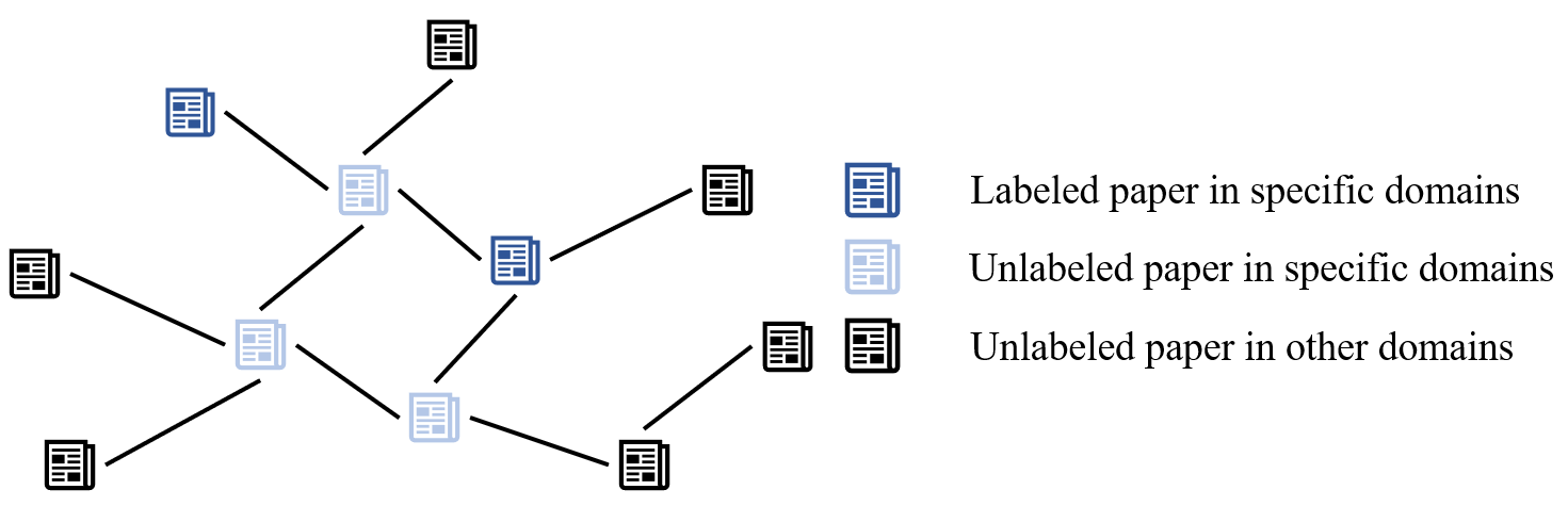
Figure 1. An example application for PU node classification: mining papers in specific domains from a citation network.

Motivated by the above limitations, in this paper, we propose to make use of graph structures for PU node classification. We first propose a novel loss function, referred as distance-aware PU loss, to introduce more accurate supervision. We also consider using graph structure as a regularization to encourage similar representations for neighboring nodes. Theoretical analysis demonstrates that minimizing our proposed loss also leads to minimizing the expected loss with both positive and negative labeled data. Empirical results on different graph data sets demonstrate the effectiveness of the proposed method.

2. Related Work

2.1. Learning from Graph-structured Data

Graph Neural Networks (GNNs) have emerged as a popular approach for learning from graph-structured data. The key idea is to leverage both node features and graph structures for node representations. At each layer of a GNN, node representations are updated by aggregating the representations of neighboring nodes. After $k$ layers of aggregation, the node representations can capture the information of their $k$-hop neighborhoods, providing richer information for node classification. Several GNN architectures have been proposed based on the general idea of neighbor aggregation (Kipf and Welling, 2017; Veličković et al., 2018; Xu et al., 2019). For example, Graph Convolutional Network (GCN) (Kipf and Welling, 2017) simplifies neighborhood aggregation through graph convolution, similar to the convolution operation for images. Graph Attention Network (GAT) (Veličković et al., 2018) applies self-attention mechanism to graph convolution, allowing the model to focus on the most relevant neighbors for each node. Graph Isomorphism Network (GIN) (Xu et al., 2019) learns more powerful representations from graph structures by incorporating permutation-invariant operations.

2.2. Positive-Unlabeled Learning

Positive-unlabeled (PU) learning refers to a special case of binary classification problem where part of training data is labeled as positive, and the rest unlabeled data can be either positive or negative. Existing PU learning methods can be broadly categorized into two approaches: prior-based methods and pseudo-label-based methods.

Prior-based methods assume the knowledge of the class prior, i.e., the proportion of positive samples in unlabeled samples, and use it to design special loss functions for PU learning. Examples include uPU (du Plessis et al., 2014), nnPU (Kiryo et al., 2017) and Dist-PU (Zhao et al., 2022), which have different forms of loss functions based on different assumptions. Other works, sush as (Chen et al., 2020; Gong et al., 2022), introduce other types of supervision to PU learning, e.g., model distillation with self-paced curriculum in (Chen et al., 2020).

In contrast, pseudo-label-based methods use two heuristic steps: first, identifying reliable negative samples from the unlabeled data, and then performing (semi-)supervised learning with additional pseudo labels. For example, PUbN (Hsieh et al., 2019) uses a model pretrained by nnPU to recognize high-confidence negative samples in the unlabeled data. PULNS (Luo et al., 2021) incorporates reinforcement learning to obtain an effective negative sample selector.

3. Methodology

For a graph $\mathcal{G}=(\mathcal{V},\mathcal{E},\mathbf{X})$, we use $\mathcal{V}=\{v_{1},\dots,v_{N}\}$ to denote the set of $N$ nodes, $\mathcal{E}\subseteq\mathcal{V}\times\mathcal{V}$ to denote the set of edges, and $\mathbf{X}=\{\mathbf{x}_{1},\dots,\mathbf{x}_{N}\}$ to denote the set of node attributes, with $\mathbf{x}_{i}$ being the attributes for node $v_{i}$. Denote the adjacency matrix by $\mathbf{A}\in\mathbb{R}^{N\times N}$, where $\mathbf{A}_{ij}=1$ if nodes ${v}_{i}$ and ${v}_{j}$ are connected, and 0 otherwise. Let $\mathcal{V}_{L}$ be the set of labeled positive nodes, and $\mathcal{V}_{U}=\mathcal{V}-\mathcal{V}_{L}$ be the set of unlabeled nodes. With these notations, the problem of PU node classification can be defined as follows.

Problem 1.

Given a graph $\mathcal{G}=(\mathcal{V},\mathcal{E},\mathbf{X})$ with a set of positively-labeled nodes $\mathcal{V}_{L}$, we want to learn a model $f$ (a GNN here) which predicts the true labels $\hat{\mathcal{Y}}_{U}$ of the unlabeled nodes $\mathcal{V}_{U}$, i.e.,

$$f(\mathcal{G},\mathcal{V}_{L},\mathcal{V}_{U})\rightarrow\mathcal{\hat{Y}}_{U}.$$

An example is illustrated in Figure 1, which aims to find papers in specific domains from a citation network. $\mathcal{V}_{L}$ contains papers that are known in these domains, while $\mathcal{V}_{U}$ contains papers whose domains are unknown. Compared to standard PU learning, a critical difference of PU node classification is the graph structure. In particular, homophily, i.e., connected nodes are more likely to belong to the same class, has been observed in many graph applications. For instance, in an academic network (Tang et al., 2008), papers are more likely to cite papers in the same field. In an epidemic network (Panagopoulos et al., 2021), neighbors of positive (affected) nodes are also more likely to be positive. Nevertheless, such information has been ignored by previous works on PU node classification (Wu et al., 2021; Yoo et al., 2021), which simply use the general PU loss for node classification.

To address this problem, in this section we consider leveraging the graph structure to provide more supervision for model training. Specifically, we propose the positive-unlabeled GNN (PU-GNN) with a distance-aware PU loss (section 3.1) as well as a regularizer from graph structure (section 3.2) to help model training.

3.1. Distance-aware PU Loss

There have been many works on designing special loss functions for PU learning (du Plessis et al., 2014; Kiryo et al., 2017; Zhao et al., 2022). One of the state-of-the-art work, Dist-PU (Zhao et al., 2022), defines the loss as follows:

(1) $$\mathcal{L}_{\text{Dist-PU}}\!=\!2\pi_{P}\left|\frac{1}{n_{L}}\!\sum\nolimits_{v_{i}\in\mathcal{V}_{L}}\hat{y}_{i}\!-\!1\right|+\left|\frac{1}{n_{U}}\!\sum\nolimits_{v_{i}\in\mathcal{V}_{U}}\hat{y}_{i}\!-\!\pi_{P}\right|,$$

where $n_{L}=|\mathcal{V}_{L}|$ denotes the number of labeled nodes, $n_{U}=|\mathcal{V}_{U}|$ denotes the number of unlabeled nodes, and $\pi_{P}$ is the prior probability for the positive class. A critical shortcoming of existing works like (1) is the ignorance of structural information for PU learning on graph. Therefore, in the following, we introduce how to integrate graph structure into the design of loss functions.

Consider a graph with only one positive node, while all other nodes are unlabeled. From homophily, the connected nodes are more likely to belong to the same class, and the influence of the only positive node should decrease with its distance to other nodes. As such, the distance to this positive node can help determine the node label: the closer an unlabeled node is to the positive node, the more likely it is to belong to the positive class.

When the graph has multiple positive nodes, a simple extension is to consider the distance of each unlabeled node to its nearest positive node. Mathematically, let $\text{dist}(v,v^{\prime})$ be the shortest-path distance between two nodes $v$ and $v^{\prime}$. We first propose to split all the unlabeled nodes in $\mathcal{V}_{U}$ into two subsets $\hat{\mathcal{V}}_{U}$ and $\breve{\mathcal{V}}_{U}$:

$$\hat{\mathcal{V}}_{U}=\Big{\{}v:v\in\mathcal{V}_{U},\min\nolimits_{v^{\prime}\in\mathcal{V}_{L}}\text{dist}(v,v^{\prime})\leq\delta\Big{\}},\quad\breve{\mathcal{V}}_{U}=\mathcal{V}_{U}\setminus\hat{\mathcal{V}}_{U},$$

where $\delta$ is a given threshold. Based on the above two subsets, we propose the following loss function for PU node classification:

$$\small\mathcal{L}_{\mathcal{G}}= 2\Big{(}\hat{\pi}_{P}+\breve{\pi}_{P}\Big{)}\Big{|}\frac{1}{n_{L}}\!\sum\nolimits_{v_{i}\in\mathcal{V}_{L}}\!\hat{y}_{i}\!-\!1\Big{|}$$

(2) $$+\Big{|}\frac{1}{\hat{n}_{U}}\!\sum\nolimits_{v_{i}\in\hat{\mathcal{V}}_{U}}\!\hat{y}_{i}\!-\!\hat{\pi}_{P}\Big{|}+\Big{|}\frac{1}{\breve{n}_{U}}\!\sum\nolimits_{v_{i}\in\breve{\mathcal{V}}_{U}}\!\hat{y}_{i}\!-\!\breve{\pi}_{P}\Big{|},$$

where $n_{L}=|\mathcal{V}_{L}|$, $\hat{n}_{U}=|\hat{\mathcal{V}}_{U}|,\breve{n}_{U}=|\breve{\mathcal{V}}_{U}|$, $\hat{\pi}_{P}$ (resp. $\breve{\pi}_{P}$) is the proportion of positive samples in $\hat{\mathcal{V}}_{U}$ (resp. $\breve{\mathcal{V}}_{U}$), and $\hat{y}_{i}$ is the prediction score for node $i$. Naturally, the choice of $\hat{\pi}_{P}$ and $\breve{\pi}_{P}$ should satisfy $\hat{\pi}_{P}>\breve{\pi}_{P}$, as nodes closer to labeled positive nodes should have higher probability of being positive. We note that each term in (2) corresponds to a set of nodes ($\mathcal{V}_{L}$, $\hat{\mathcal{V}}_{U}$ and $\breve{\mathcal{V}}_{U}$). With only one unlabeled data set (i.e., not using structural information), the loss in (2) reduces to the Dist-PU loss in (1). Similar to (Zhao et al., 2022), the following proposition shows that the proposed loss provides an upper bound on the training loss with ground-truth labels (both positive and negative).

Proposition 3.1.

Denote the distribution of positive (resp. negative) nodes as $p_{P}(v)$ (resp. $p_{N}(v)$). For each node $v_{i}$, denote its prediction as $y_{i}$, and define the expected loss on the whole graph as $\hat{\mathcal{L}}=\pi_{P}|\mathbb{E}_{v_{i}\sim p_{P}(v_{i})}\hat{y}_{i}-1|+(1-\pi_{P})|\mathbb{E}_{v_{i}\sim p_{N}(v_{i})}\hat{y}_{i}|$. Then for a class of bounded functions $F$ with VC dimension $V$, with probability at least 1 - $\delta$, we have:

$$\small\hat{\mathcal{L}}\leq\mathcal{L}_{\mathcal{G}} +8\pi_{P}C\sqrt{V/n_{L}}+12\pi_{P}\sqrt{\log(4/\delta)/(2n_{L})}$$

$$+4C\sqrt{V/(\hat{n}_{U}+\breve{n}_{U})}+6\sqrt{\log(4/\delta)/(2\hat{n}_{U}+2\breve{n}_{U})},$$

The above proposition demonstrates that minimizing $\mathcal{L}_{\mathcal{G}}$ also leads to minimizing the expected loss $\hat{\mathcal{L}}$ by minimizing the upper bound on the right hand side, though we do not know any negatively-labeled nodes in practice.

3.2. Structural Regularization

While distance-aware PU loss assigns different priors among unlabeled nodes, it still overlooks the pairwise relations between nodes. As such, we propose a regularization term based on the graph structure to encourage similar representations and final predictions for neighboring nodes.

Let $P(v_{i})$ be the uniform distribution on all nodes that are not node $v_{i}$’s neighbors. For each edge $(i,j)$ with $\mathbf{A}_{ij}=1$, we randomly sample $K$ nodes from $P(v_{i})$ as negative samples. The structural regularizer $\mathcal{R}_{S}$ is then defined as:

(3) $$\small\mathcal{R}_{S}\!=\!\sum\nolimits_{v_{i}\in\mathcal{V}}\sum\nolimits_{v_{j}\in\mathcal{N}(v_{i})}\Big{(}(\mathbf{S}_{ij}\!-\!1)^{2}\!+\!\sum\nolimits_{k=1}^{K}\mathbb{E}_{v_{k}\sim P(v_{i})}(\mathbf{S}_{ik}\!-\!0)^{2}\Big{)},$$

where $\mathbf{S}_{ij}=\sigma(\mathbf{z}_{i}^{\top}\mathbf{z}_{j})$ is the similarity between node $v_{i}$ and $v_{j}$’s representations $\mathbf{z}_{i}$ and $\mathbf{z}_{j}$, $\sigma(\cdot)$ is the sigmoid function, and $\mathcal{N}(v_{i})$ is the set of node $v_{i}$’s neighboring nodes. Minimizing the first term $(\mathbf{S}_{ij}\!-\!1)^{2}$ in (3) encourages neighboring nodes ($v_{i}$ and $v_{j}$) to have similar representations, while minimizing the second term $\sum\nolimits_{k=1}^{K}\mathbb{E}_{v_{k}\sim P_{n}(v_{i})}(\mathbf{S}_{ik}\!-\!0)^{2}$ in (3) encourages node $v_{i}$ to have different representations from its non-neighboring nodes $v_{k}$’s.

Combining (3) and (2), the final objective $\mathcal{L}$ is given by $\mathcal{L}=\mathcal{L}_{\mathcal{G}}+\alpha\mathcal{R}_{S}$, where $\alpha$ is used to balance the contribution of structural regularization $\mathcal{R}_{S}$.

4. Experiments

4.1. Experimental Setup

We conducted experiments on four node classification data sets: Cora, Citeseer, Pubmed and DBLP, which are popularly used in literature (Kipf and Welling, 2017; Veličković et al., 2018; Wu et al., 2021; Yoo et al., 2021). The data set statistics are summarized in Table 1. We follow the splits in (Sen et al., 2008), but merge their validation and test splits into a single test split. To transform these datasets into binary classification tasks, we follow the approach in (Wu et al., 2021), where we treated a subset of the classes as positive and the others as negative. The resulting numbers of positive and negative samples are shown in Table 1. To convert these datasets into PU learning problems, we randomly selected a small proportion of positive nodes (called label ratio) in the training set and removed the labels of the rest. We experimented with different label ratios, including $\{0.001,0.002,0.005,0.01\}$, to evaluate the performance of our approach under varying levels of label scarcity.

Table 1. Statistics of datasets.

		Cora	Citeseer	Pubmed	DBLP
# nodes	total	2,708	3,327	19,717	17,716
	positive	1,244	1,369	7,875	7,920
	negative	1,464	1,958	11,842	9,796
	training	271	333	1,971	1,772
	testing	2,437	2,994	17,746	15,944

For the proposed method, we set $\alpha=0.01$, threshold $\delta=3$, the number of negative samples $K=50$, and the class priors $\hat{\pi}_{P}=0.6,\breve{\pi}_{P}=0.3$. We use a two-layer GCN with hidden dimension 16 as the backbone. As will be demonstrated by experiments later, the proposed method is not sensitive to these hyper-parameters and it is easy to pick up proper values.

The proposed method is compared with the following baselines: (i) naive GCN, which considers all unlabeled nodes as negative; (ii) GCN with nnPU loss (Kiryo et al., 2017); (iii) GCN with Dist-PU loss (Zhao et al., 2022); (iv) LSDAN (Wu et al., 2021), which introduces long-range dependency with the nnPU loss (Kiryo et al., 2017); and (v) GRAB (Yoo et al., 2021), which models the given graph as a Markov network and uses loopy belief propagation (LBP) to estimate the label distribution of unlabeled nodes. As in (Kipf and Welling, 2017; Kiryo et al., 2017; Zhao et al., 2022), we use macro F1 score (%) on the testing nodes as performance measure. The experiment is repeated 5 times, and we report the average performance with standard deviation.

4.2. Node Classification Performance

Table 2 shows macro F1 scores (%) on the testing set with different label ratios. As can be seen, using the PU loss improves the naive GCN baseline much, and Dist-PU significantly outperforms nnPU in most cases. Methods specific to PU node classification (LSDAN (Wu et al., 2021) and GRAB (Yoo et al., 2021)) generally have better performances than Dist-PU, and their performances are comparable to each other. The proposed PU-GNN achieves the best performance for almost all data sets and label ratios, demonstrating that graph structure plays a critical role in the loss design for PU node classification.

Table 2. Macro F1 score (%) on the testing set with different label ratio $\{0.001,0.002,0.005,0.01\}$. GCN is used as the backbone network for all methods.

Data set	Method	0.001	0.002	0.005	0.01
Cora	naive	78.1$\pm$0.1	78.1$\pm$0.1	78.1$\pm$0.1	78.1$\pm$0.1
	nnPU	80.3$\pm$0.2	80.9$\pm$0.3	83.9$\pm$0.4	85.6$\pm$0.2
	Dist-PU	82.1$\pm$0.2	82.7$\pm$0.3	86.6$\pm$0.3	87.4$\pm$0.2
	LSDAN	81.8$\pm$0.2	82.8$\pm$0.2	86.7$\pm$0.3	87.6$\pm$0.2
	GRAB	82.5$\pm$0.3	84.4$\pm$0.3	86.5$\pm$0.2	87.5$\pm$0.2
	PU-GNN	84.8$\pm$0.3	86.0$\pm$0.3	87.3$\pm$0.2	88.3$\pm$0.2
Pubmed	naive	57.1$\pm$0.1	57.1$\pm$0.1	57.1$\pm$0.1	57.1$\pm$0.1
	nnPU	63.6$\pm$0.4	65.7$\pm$0.3	70.5$\pm$0.3	73.8$\pm$0.3
	Dist-PU	63.3$\pm$0.3	67.1$\pm$0.2	72.2$\pm$0.2	74.3$\pm$0.3
	LSDAN	69.6$\pm$0.4	71.4$\pm$0.3	72.7$\pm$0.2	75.1$\pm$0.2
	GRAB	70.6$\pm$0.3	71.6$\pm$0.4	73.3$\pm$0.2	75.0$\pm$0.3
	PU-GNN	73.0$\pm$0.4	73.5$\pm$0.3	74.0$\pm$0.2	74.8$\pm$0.2
Citeseer	naive	61.0$\pm$0.1	61.0$\pm$0.1	61.0$\pm$0.1	61.0$\pm$0.1
	nnPU	61.2$\pm$0.4	62.2$\pm$0.3	62.7$\pm$0.2	63.8$\pm$0.2
	Dist-PU	61.4$\pm$0.4	62.2$\pm$0.2	63.5$\pm$0.3	64.6$\pm$0.2
	LSDAN	62.7$\pm$0.3	63.6$\pm$0.2	65.6$\pm$0.3	70.5$\pm$0.3
	GRAB	61.8$\pm$0.4	62.6$\pm$0.3	65.2$\pm$0.3	69.7$\pm$0.4
	PU-GNN	64.5$\pm$0.4	64.7$\pm$0.2	65.8$\pm$0.3	73.0$\pm$0.3
DBLP	naive	34.4$\pm$0.2	34.4$\pm$0.2	34.4$\pm$0.2	34.6$\pm$0.3
	nnPU	83.4$\pm$0.3	83.9$\pm$0.2	85.4$\pm$0.3	86.7$\pm$0.4
	Dist-PU	83.8$\pm$0.2	84.1$\pm$0.3	86.8$\pm$0.2	87.3$\pm$0.3
	LSDAN	85.3$\pm$0.2	85.6$\pm$0.2	86.8$\pm$0.2	87.8$\pm$0.2
	GRAB	85.0$\pm$0.2	85.7$\pm$0.3	86.8$\pm$0.2	87.8$\pm$0.2
	PU-GNN	86.5$\pm$0.1	86.6$\pm$0.2	87.2$\pm$0.4	87.8$\pm$0.3

4.3. Ablation Study

4.3.1. Contribution of Each Component

We first study the usefulness of the proposed distance-aware PU loss (abbreviated as “PU loss”) and structural regularization (abbreviated as “struct reg”). Table 3 shows macro F1 scores (%) on the testing set of Cora for GCN and different variants of the proposed PU-GNN with different label ratios. As can be seen, both the distance-aware PU loss and structural regularization are critical to model performance. Moreover, with more labels, using only distance-aware PU loss achieves closer performance with the full PU-GNN model, and even slightly outperforms the full PU-GNN model at the end. This can be explained as more labeled nodes provide more accurate supervision, leading to better performances even when only the distance-aware PU loss is used.

Table 3. Macro F1 score (%) on the testing set with different variants of PU-GNN. Cora data set is used.

Label ratio	GCN	PU-GNN
		($\checkmark$ struct reg, $\checkmark$ PU loss)	84.8$\pm$0.3
0.001	78.1$\pm$0.1	($\checkmark$ struct reg, ✗  PU loss)	80.2$\pm$0.2
		(✗  struct reg, $\checkmark$ PU loss)	83.2$\pm$0.3
		($\checkmark$ struct reg, $\checkmark$ PU loss)	86.0$\pm$0.3
0.002	78.1$\pm$0.1	($\checkmark$ struct reg, ✗  PU loss)	80.6$\pm$0.3
		(✗  struct reg, $\checkmark$ PU loss)	85.0$\pm$0.4
		($\checkmark$ struct reg, $\checkmark$ PU loss)	87.3$\pm$0.2
0.005	78.1$\pm$0.1	($\checkmark$ struct reg, ✗  PU loss)	81.6$\pm$0.2
		(✗  struct reg, $\checkmark$ PU loss)	86.7$\pm$0.3
		($\checkmark$ struct reg, $\checkmark$ PU loss)	88.3$\pm$0.2
0.01	78.1$\pm$0.1	($\checkmark$ struct reg, ✗  PU loss)	83.4$\pm$0.3
		(✗  struct reg, $\checkmark$ PU loss)	88.7$\pm$0.3

4.3.2. Hyper-parameter Sensitivity

Here, we study the proposed method’s sensitivity to hyper-parameters. We use the Cora data set with label ratio 0.002. For $\hat{\pi}_{P}$ and $\breve{\pi}_{P}$, we should have $\hat{\pi}_{P},\breve{\pi}_{P}\in(0,1)$ and $\hat{\pi}_{P}\geq\breve{\pi}_{P}$, since they refer to the proportion of positive samples in a given node set. And for the threshold $\delta$ in (2), we vary it in $\{1,2,3,4,5\}$. We do not consider $\delta\geq 6$ as for all the three data sets, the largest distance between any pairs of nodes is not larger than $6$, hence using $\delta\geq 6$ will make $\breve{\mathcal{V}}_{U}$ be an empty set and reduce to the Dist-PU loss.

Table 4 shows macro F1 scores (%) on the testing set with different positive priors. We can see that our method attains satisfying performance across a wide range of values around $\hat{\pi}_{P}=0.6$ and $\breve{\pi}_{P}=0.3$, where performances better than any baseline methods in Table 2 are all highlighted.

Table 4. Macro F1 score (%) on the testing set with different $\hat{\pi}_{P}$ and $\breve{\pi}_{P}$’s. Cora data set is used.

	0.5	0.6	0.7	0.8	0.9
0.1	84.6$\pm$0.3	85.3$\pm$0.2	84.6$\pm$0.2	83.8$\pm$0.4	83.4$\pm$0.3
0.2	84.6$\pm$0.3	85.3$\pm$0.2	85.2$\pm$0.3	84.0$\pm$0.3	83.4$\pm$0.3
0.3	85.7$\pm$0.3	86.0$\pm$0.3	85.9$\pm$0.3	84.8$\pm$0.3	84.4$\pm$0.2
0.4	84.0$\pm$0.3	85.9$\pm$0.3	83.7$\pm$0.4	84.0$\pm$0.4	83.4$\pm$0.3

Table 5 compares the macro F1 scores (%) on the testing set with different thresholds $\delta$. As can be seen, setting $\delta$ too small (resp. too large) will make set $\hat{\mathcal{V}}_{U}$ (resp. $\breve{\mathcal{V}}_{U}$) only have a small amount of nodes, leading to similar performances with Dist-PU loss (82.7$\pm$0.3). The proposed method achieves good performances when $\delta$ is chosen from 2 or 3.

Table 5. Macro F1 score (%) on the testing set with different $\delta$’s. Cora data set is used.

$\delta$	1	2	3	4	5
F1 score (%)	83.0$\pm$0.4	85.8$\pm$0.2	86.0$\pm$0.3	83.2$\pm$0.3	82.8$\pm$0.3

5. Conclusion

In this paper, we propose to utilize graph structures to benefit PU node classification. We first propose a distance-aware loss function, which uses homophily in graph structure to introduce more accurate supervision for unlabeled nodes. Theoretical analysis demonstrates that minimizing the proposed loss leads to minimizing the expected loss with both positive and negative labels. We also propose a regularizer based on graph structure to further improve model performances. Empirical results across different data sets demonstrate the effectiveness of our proposed method. For future works, we may consider generalize the proposed method from homophily to heterophily for node classification.

References

- (1)
- Berthelot et al. (2019) David Berthelot, Nicholas Carlini, Ian Goodfellow, Nicolas Papernot, Avital Oliver, and Colin A Raffel. 2019. Mixmatch: A holistic approach to semi-supervised learning. NeurIPS (2019).
- Chen et al. (2020) Xuxi Chen, Wuyang Chen, Tianlong Chen, Ye Yuan, Chen Gong, Kewei Chen, and Zhangyang Wang. 2020. Self-pu: Self boosted and calibrated positive-unlabeled training. In ICML.
- Dai et al. (2020) Rui Dai, Shenkun Xu, Qian Gu, Chenguang Ji, , and Kaikui Liu. 2020. Hybrid Spatio-Temporal Graph Convolutional Network: Improving Traffic Prediction with Navigation Data.. In SIGKDD.
- du Plessis et al. (2014) Marthinus Christoffel du Plessis, Gang Niu, and Masashi Sugiyama. 2014. Analysis of learning from positive and unlabeled data. In NeurIPS.
- Fang et al. (2012) Yuan Fang, Bo-June Hsu, and Kevin Chen-Chuan Chang. 2012. Confidence-aware graph regularization with heterogeneous pairwise features. In SIGIR.
- Gong et al. (2022) Chen Gong, Qizhou Wang, Tongliang Liu, Bo Han, Jane J You, Jian Yang, and Dacheng Tao. 2022. Instance-dependent positive and unlabeled learning with labeling bias estimation. TPAMI 44, 8 (2022), 4163–4177.
- Hsieh et al. (2019) Yu-Guan Hsieh, Gang Niu, and Masashi Sugiyama. 2019. Classification from positive, unlabeled and biased negative data. In ICML.
- Kipf and Welling (2017) Thomas N Kipf and Max Welling. 2017. Semi-supervised classification with graph convolutional networks. In ICLR.
- Kiryo et al. (2017) Ryuichi Kiryo, Gang Niu, Marthinus Christoffel du Plessis, and Masashi Sugiyama. 2017. Positive-unlabeled learning with non-negative risk estimator. In NeurIPS.
- Luo et al. (2021) Chuan Luo, Pu Zhao, Chen Chen, Bo Qiao, Chao Du, Hongyu Zhang, Wei Wu, Shaowei Cai, Bing He, Saravanakumar Rajmohan, and Qingwei Lin. 2021. PULNS: positive-unlabeled learning with effective negative sample selector. In AAAI.
- Panagopoulos et al. (2021) George Panagopoulos, Giannis Nikolentzos, and Michalis Vazirgiannis. 2021. Transfer graph neural networks for pandemic forecasting. In AAAI.
- Seah et al. (2018) Boon-Siew Seah, Aixin Sun, and Sourav S Bhowmick. 2018. Killing two birds with one stone: Concurrent ranking of tags and comments of social images. In SIGIR.
- Sen et al. (2008) Prithviraj Sen, Galileo Namata, Mustafa Bilgic, Lise Getoor, Brian Galligher, and Tina Eliassi-Rad. 2008. Collective classification in network data. AI magazine 29, 3 (2008), 93–93.
- Tang et al. (2008) Jie Tang, Jing Zhang, Limin Yao, Juanzi Li, Li Zhang, and Zhong Su. 2008. Arnetminer: extraction and mining of academic social networks. In SIGKDD. 990–998.
- Veličković et al. (2018) Petar Veličković, Guillem Cucurull, Arantxa Casanova, Adriana Romero, Pietro Lio, and Yoshua Bengio. 2018. Graph attention networks. ICLR.
- Wang et al. (2019) Weiqing Wang, Hongzhi Yin, Xingzhong Du, Wen Hua, Yongjun Li, and Quoc Viet Hung Nguyen. 2019. Online user representation learning across heterogeneous social networks. In SIGIR.
- Wu et al. (2021) Man Wu, Shirui Pan, Lan Du, and Xingquan Zhu. 2021. Learning graph neural networks with positive and unlabeled nodes. TKDD 15, 6 (2021), 1–25.
- Xu et al. (2019) Keyulu Xu, Weihua Hu, Jure Leskovec, and Stefanie Jegelka. 2019. How powerful are graph neural networks?. In ICLR.
- Yoo et al. (2021) Jaemin Yoo, Junghun Kim, Hoyoung Yoon, Geonsoo Kim, Changwon Jang, and U Kang. 2021. Accurate graph-based PU learning without class prior. In ICDM.
- Zhao et al. (2022) Yunrui Zhao, Qianqian Xu, Yangbangyan Jiang, Peisong Wen, and Qingming Huang. 2022. Dist-PU: Positive-Unlabeled Learning from a Label Distribution Perspective. In CVPR.
- Zhou (2021) Zhi-Hua Zhou. 2021. Semi-supervised learning. Machine Learning (2021), 315–341.