Multiple and weak Markov properties in Hilbert spaces with applications to fractional stochastic evolution equations

Abstract.

We define various higher-order Markov properties for stochastic processes $(X(t))_{t\in\mathbb{T}}$, indexed by an interval $\mathbb{T}\subseteq\mathbb{R}$ and taking values in a real and separable Hilbert space $U$. We furthermore investigate the relations between them. In particular, for solutions to the stochastic evolution equation $\mathcal{L}X=\dot{W}^{Q}\!$, where $\mathcal{L}$ is a linear operator acting on functions mapping from $\mathbb{T}$ to $U$ and $(\dot{W}^{Q}(t))_{t\in\mathbb{T}}$ is the formal derivative of a $U$-valued (cylindrical) $Q$-Wiener process, we prove necessary and sufficient conditions for the weakest Markov property via locality of the precision operator $\mathcal{L}^{*}\!\mathcal{L}$.

As an application, we consider the space–time fractional parabolic operator $\mathcal{L}={(\partial_{t}+A)^{\gamma}}$ of order ${\gamma\in(1/2,\infty)}$, where $-A$ is a linear operator generating a $C_{0}$-semigroup on $U$. We prove that the resulting solution process satisfies an $N$th order Markov property if $\gamma=N\in\mathbb{N}$ and show that a necessary condition for the weakest Markov property is generally not satisfied if $\gamma\notin\mathbb{N}$. The relevance of this class of processes is twofold: Firstly, it can be seen as a spatiotemporal generalization of Whittle–Matérn Gaussian random fields if $U=L^{2}(\mathcal{D})$ for a spatial domain $\mathcal{D}\subseteq\mathbb{R}^{d}\!$. Secondly, we show that a $U$-valued analog to the fractional Brownian motion with Hurst parameter $H\in(0,1)$ can be obtained as the limiting case of $\mathcal{L}=(\partial_{t}+\varepsilon\,\mathrm{Id}_{U})^{H+\frac{1}{2}}$ for $\varepsilon\downarrow 0$.

1. Introduction

1.1. Background and motivation

Gaussian Markov random fields play an important role for various applications, such as the analysis of time series or longitudinal data, image processing and spatial statistics, see e.g. [42, Section 1.3]. The latter focuses on the statistical modeling of spatial or spatiotemporal dependence in data collected from phenomena encountered in disciplines such as climatology [1], epidemiology [26] and neuroimaging [34]. The popularity of Gaussian Markov random fields among the larger class of Gaussian random fields is a consequence of their additional conditional independence properties, which entail a sparse precision structure and facilitate efficient computational methods for statistical inference. In particular, hierarchical models based on Gaussian Markov random fields allow for efficient Bayesian inference using Markov chain Monte Carlo methods, see e.g. [42, Section 4.1].

Since a Gaussian process is fully characterized by its second-order structure, i.e., the mean and covariance function, a natural way to specify its distribution is to choose a suitable second-order structure. Alternatively, the dynamics of Gaussian random fields defined on a Euclidean domain $\mathcal{D}\subseteq\mathbb{R}^{d}$ can be specified by means of stochastic partial differential equations (SPDEs), such as the white noise $(\mathcal{W}(x))_{x\in\mathcal{D}}$ driven equation

$$LX(x)=\mathcal{W}(x),\quad x\in\mathcal{D}.$$ (1.1)

Here, $L$ is a linear operator acting on real-valued functions defined on $\mathcal{D}$. A spatial Gaussian random field $(X(x))_{x\in\mathcal{D}}$ is said to have the Markov property if the subcollections $(X(x))_{x\in\mathcal{D}_{1}}$ and $(X(x))_{x\in\mathcal{D}_{2}}$ corresponding to pairs of disjoint subdomains $\mathcal{D}_{1},\mathcal{D}_{2}\subseteq\mathcal{D}$ are independent conditional on $(X(x))_{x\in\mathcal{D}^{\prime}}$ for some non-trivial ‘splitting’ set $\mathcal{D}^{\prime}\subseteq\mathcal{D}$ separating the two. The precise specification of these sets, which respectively carry the intuitive interpretations of past, future and present, leads to various definitions of the Markov property. According to the theory of Rozanov [41], a real-valued Gaussian random field satisfying (1.1) has such a Markov property if and only if its precision operator $L^{*}\!L$ is local, where $L^{*}$ denotes the adjoint of $L$.

An important example in spatial statistics is the choice of a fractional-order differential operator $L:=\tau(\kappa^{2}-\Delta)^{\beta}$ in (1.1), where $\Delta$ is the Laplacian, $\mathcal{W}$ is Gaussian white noise and $\tau,\kappa,\beta\in(0,\infty)$. Whittle [47] observed that the covariance function of the stationary solution $(X(x))_{x\in\mathcal{D}}$ to (1.1) with $\mathcal{D}=\mathbb{R}^{d}$ then belongs to the widely used Matérn covariance class [33]. This observation motivated the SPDE approach for spatial statistical modeling proposed by Lindgren, Rue and Lindström [29]. Here, one considers (1.1) on a bounded Euclidean domain $\mathcal{D}\subsetneq\mathbb{R}^{d}$, augmented with boundary conditions, and approximates the resulting Whittle–Matérn fields by means of efficient numerical methods available for (S)PDEs. Owing to its ease of generalization and its computational efficiency as compared to covariance-based techniques, this approach has gained widespread popularity, see e.g. [5, 6, 7, 17, 28, 43]. Since in this case the precision operator is given by $L^{*}\!L=\tau^{2}(\kappa^{2}-\Delta)^{2\beta}\!$, we find that Whittle–Matérn fields are Gaussian Markov random fields in the sense of Rozanov [41] precisely when $2\beta\in\mathbb{N}$.

Recently, extensions of the SPDE approach incorporating time dependence have been discussed. A class of space–time equations which has been proposed in this context is

$$(\partial_{t}+L)^{\gamma}X(t,x)=\dot{\mathcal{W}}^{Q}(t,x),\quad(t,x)\in\mathbb{T}\times\mathcal{D},$$ (1.2)

where $\mathbb{T}\subseteq\mathbb{R}$ represents a time interval and $\dot{\mathcal{W}}^{Q}$ is spatiotemporal Gaussian noise, which is spatially colored by an operator $Q$, see [24, 27]. In particular, it has been shown in [24] that equation (1.2) extends the Matérn model in terms of spatial marginal covariance, and that the interplay of its parameters governs smoothness in space and time as well as the degree of separability.

Spatiotemporal random fields can be viewed as $U$-valued stochastic processes by letting a Hilbert space $U$ encode the spatial variable, so that (1.2) corresponds to a stochastic fractional evolution equation of the form

$$(\partial_{t}+A)^{\gamma}X(t)=\dot{W}^{Q}(t),\quad t\in\mathbb{T}.$$ (1.3)

The (temporal) Markov property of solutions to (1.2) is then equivalent to that of the $U$-valued solution process $(X(t))_{t\in\mathbb{T}}$, where the Markov behavior is considered with respect to the index set $\mathbb{T}$. Moreover, viewing (1.3) as a special case of

$$\mathcal{L}X(t)=\dot{W}^{Q}(t),\quad t\in\mathbb{T},$$ (1.4)

where $\mathcal{L}$ is now a linear operator acting on functions from $\mathbb{T}$ to $U$, the theory of Rozanov [41] suggests that locality of the precision operator $\mathcal{L}^{*}\!\mathcal{L}$, also acting on functions $f\colon\mathbb{T}\to U$, can be used to characterize temporal Markov behavior of the solution $X$.

1.2. Contributions

In this work we define simple, multiple ($N$-ple for $N\in\mathbb{N}$) and weak Markov properties for stochastic processes which take values in a Hilbert space $U$. These definitions generalize those appearing for instance in [18, 40, 41] for real-valued processes to infinite dimensions, see Definitions 3.1, 3.3 and 3.5, respectively. Besides gathering them in once place, we establish their interrelations, see Proposition 3.6 and Remark 3.7. The main results are Theorems 3.8 and 3.10, which give necessary and sufficient conditions, in terms of the precision operator $\mathcal{L}^{*}\!\mathcal{L}$, for the weakest notion of Markovianity for a $U$-valued Gaussian process defined via (1.4). These results are proven by a non-trivial extension of the theory by Rozanov [41, Chapters 2 and 3] from the real-valued to the $U$-valued setting.

In order to consider the more concrete class of processes defined via (1.3), we construct a stochastic integral for deterministic operator-valued integrands defined on the whole of $\mathbb{R}$ with respect to a two-sided (cylindrical) $Q$-Wiener process $(W^{Q}(t))_{t\in\mathbb{R}}$, see Subsection 2.2. We employ this stochastic integral to define the mild solution process $Z_{\gamma}=(Z_{\gamma}(t))_{t\in\mathbb{R}}$ to (1.3) on $\mathbb{T}=\mathbb{R}$, see Definition 4.5. Our rigorous definition of the fractional space–time operator $(\partial_{t}+A)^{\gamma}$ for $\gamma\in\mathbb{R}$, see Definition 4.3, extends the Weyl fractional calculus in the sense that one recovers the Weyl fractional derivatives and integrals defined in [22, Section 2.3] upon specializing to $U=\mathbb{R}$ and $A=0$.

We show that the mild solution $Z_{\gamma}$ to (1.3) satisfies the $N$-ple Markov property if $\gamma=N\in\mathbb{N}$, see Theorem 4.9. Conversely, we use Theorem 3.8 to show that $Z_{\gamma}$ is in general not weakly Markov for $\gamma\not\in\mathbb{N}$. This complements [14, Theorem 2.7], where the authors show that any time-homogeneous $U$-valued Gaussian simple Markov process is the solution to a first-order stochastic evolution equation.

Finally, we discuss another interesting aspect of the SPDE (1.3): A fractional $Q$-Wiener process $(W_{H}^{Q}(t))_{t\in\mathbb{R}}$ with Hurst parameter $H\in(0,1)$, as defined for instance in [12], can be obtained as a limiting case of (1.3) with $\gamma=H+\frac{1}{2}$ and $A=\varepsilon\operatorname{Id}_{U}$ as $\varepsilon\downarrow 0$, see Proposition 5.3. The proof is based on a Mandelbrot–Van Ness [31] type integral representation of $W^{Q}_{H}$, again using the two-sided stochastic integral from Subsection 2.2, see Proposition 5.2. The case $H=\frac{1}{2}$ corresponds to a (non-fractional) $Q$-Wiener process and is thus Markov. Conversely, although the results of Theorems 3.8 and 3.10 do not apply directly, the above observation provides evidence that $W^{Q}_{H}$ does not satisfy a weak Markov property for $H\in(0,1)\setminus\{\frac{1}{2}\}$.

1.3. Outline

In Section 2 we begin by establishing the necessary notation, see Subsection 2.1, followed by the construction of the stochastic integral with respect to a two-sided (cylindrical) $Q$-Wiener process in Subsection 2.2. Section 3 is devoted to defining, relating and (for solutions to (1.4)) characterizing various notions of Markov behavior for $U$-valued stochastic processes. The goal of Section 4 is to define and analyze the mild solution to (1.3) on $\mathbb{T}=\mathbb{R}$. To this end, we first describe the setting and define $(\partial_{t}+A)^{\gamma}$ with $\gamma\in\mathbb{R}$ in Subsections 4.1 and 4.2, respectively, and subsequently investigate for which values of $\gamma$ the process exhibits Markov behavior in Subsection 4.4. In Section 5 we recall the definition from [12] of a $Q$-fractional Wiener process and prove a Mandelbrot–Van Ness type integral representation, which allows us to exhibit it as a limiting case of (1.3).

This article is supplemented by three appendices: Appendix A collects some definitions and facts about spaces of functions with values in a Hilbert or Banach space. It is followed by Appendix B, which contains auxiliary results relating to specific results from the main text whose statements and proofs were postponed for readability; subjects include conditional independence, filtrations indexed by $\mathbb{R}$ and the mean-square differentiability of stochastic convolutions. Appendix C is a short overview of results regarding fractional powers of linear operators and their relation to the fractional parabolic operator $(\partial_{t}+A)^{\gamma}$.

2. Preliminaries

2.1. Notation

The sets $\mathbb{N}:=\{1,2,3,\dots\}$ and $\mathbb{N}_{0}:=\mathbb{N}\cup\{0\}$ denote the positive and non-negative integers, respectively. We write $s\wedge t$ (or $s\vee t$) for the minimum (or maximum) of two real numbers $s,t\in\mathbb{R}$. Empty sums and products are assigned the values zero and one, respectively. Given two arbitrary sets $D$ and $E$, the preimage of $E_{0}\subseteq E$ under the function $f\colon D\to E$ is defined by ${f^{-1}[E_{0}]=\{f\in E_{0}\}=\{x\in D:f(x)\in E_{0}\}}$. The identity on $D$ and the indicator function of $D_{0}\subseteq D$ are respectively denoted by $\operatorname{Id}_{D}\colon D\to D$ and $\mathbf{1}_{D_{0}}\colon D\to\{0,1\}$.

Let $(U,\langle\,\cdot\,,\,\cdot\,\rangle_{U})$ and $(\widetilde{U},\langle\,\cdot\,,\,\cdot\,\rangle_{\widetilde{U}})$ denote Hilbert spaces with induced norms ${\|\cdot\|_{U}}$ and $\|\cdot\|_{\widetilde{U}}$. Banach spaces are usually denoted by $(E,\|\cdot\|_{E})$ and $(F,\|\cdot\|_{F})$. These spaces are all assumed to be real and separable.

We write ${\mathscr{L}(E;F)}$ for the Banach space of bounded linear operators equipped with the usual operator norm. The adjoint operator of $T\in\mathscr{L}(E;F)$ is denoted by ${T^{*}\in\mathscr{L}(F^{*};E^{*})}$, where $E^{*},F^{*}$ denote the dual spaces; if $T\in\mathscr{L}({U};\widetilde{U})$, then we can identify $U^{*}=U$ and $\widetilde{U}^{*}=\widetilde{U}$ via the Riesz maps, so that $T^{*}\in\mathscr{L}(\widetilde{U};{U})$. We abbreviate $\mathscr{L}(E):=\mathscr{L}(E;E)$, and similarly for the other spaces of linear operators.

We write $T\in\mathscr{L}^{+}(U)$ to indicate that $T\in\mathscr{L}(U)$ is self-adjoint positive definite, meaning that $T^{*}=T$ and there exists $\theta\in(0,\infty)$ such that $\langle Tx,x\rangle_{U}\geq\theta\|x\|_{U}^{2}$ for all $x\in U$. Let $\mathscr{L}_{2}(U;\widetilde{U})\subseteq\mathscr{L}(U;\widetilde{U})$ denote the Hilbert space of all Hilbert–Schmidt operators equipped with the inner product $\langle T,S\rangle_{\mathscr{L}_{2}(U;\widetilde{U})}:=\sum_{j\in\mathbb{N}}\langle Te_{j},Se_{j}\rangle_{\widetilde{U}}$, where $(e_{j})_{j\in\mathbb{N}}$ is any orthonormal basis for $U$. The trace of $T\in\mathscr{L}^{+}(U)$ is defined by $\operatorname{tr}T:=\sum_{j\in\mathbb{N}}\langle Te_{j},e_{j}\rangle_{U}.$ We say that $T\in\mathscr{L}(U)$ belongs to the Banach space $\mathscr{L}_{1}(U)$ of trace class operators if $\|T\|_{\mathscr{L}_{1}(U)}:=\operatorname{tr}|T|<\infty$ for $|T|:=(T^{*}T)^{\frac{1}{2}}$, using the operator square root (see e.g. [45, Proposition 8.27]) and set $\mathscr{L}_{1}^{+}(U):=\mathscr{L}^{+}(U)\cap\mathscr{L}_{1}(U)$.

A linear operator $A$ on $E$ with domain $\mathsf{D}(A)$ is denoted by ${A\colon\mathsf{D}(A)\subseteq E\to E}$; for its range we write $\mathsf{R}(A)$. We call $A$ closed if its graph $\mathsf{G}(A):={\{(x,Ax):x\in\mathsf{D}(A)\}}$ is closed with respect to the norm $\|(x,Ax)\|_{\mathsf{G}(A)}=\|x\|_{\mathsf{D}(A)}=\|x\|_{E}+\|Ax\|_{E}$, and densely defined if $\mathsf{D}(A)$ is dense in $E$. If the closure $\overline{\mathsf{G}(A)}$ is the graph of a linear operator $\overline{A}$, then we call $\overline{A}$ the closure of $A$. We write $A\subseteq\widetilde{A}$ if $\mathsf{G}(A)\subseteq\mathsf{G}(\widetilde{A})$.

Throughout this work, we assume that a complete probability space $(\Omega,\mathcal{F},\mathbb{P})$ is given, meaning that $\mathcal{F}$ contains the collection $\mathcal{N}_{\mathbb{P}}$ of $\mathbb{P}$-null sets. We abbreviate the phrase “$\mathbb{P}$-almost surely” by “$\mathbb{P}$-a.s.” In what follows, we call a function $Z\colon\Omega\to E$ an $E$-valued random variable if it is strongly $\mathbb{P}$-measurable, see Subsection A.1 in Appendix A. We write $Z\sim N(m,Q)$ if $Z$ is a $U$-valued Gaussian random variable with mean $m\in U$ and covariance operator $Q\in\mathscr{L}^{+}_{1}(U)$; its existence is guaranteed by [4, Theorem 2.3.1]. Two stochastic processes $(X(t))_{t\in\mathbb{T}}$ and $(\widetilde{X}(t))_{t\in\mathbb{T}}$ are said to be modifications of each other if $\mathbb{P}(X(t)=\widetilde{X}(t))=1$ for all $t\in\mathbb{T}$, where $\mathbb{T}=[0,\infty)$, $\mathbb{T}=[0,T]$ for some $T\in(0,\infty)$ or $\mathbb{T}=\mathbb{R}$.

Let $\mathcal{G}_{1},\mathcal{H},\mathcal{G}_{2}\subseteq\mathcal{F}$ be sub-$\sigma$-algebras of $\mathcal{F}$. The join of two $\sigma$-algebras is denoted by $\mathcal{G}_{1}\vee\mathcal{G}_{2}:=\sigma(\mathcal{G}_{1}\cup\mathcal{G}_{2})$. We write $\mathcal{G}_{1}\perp\!\!\!\perp\mathcal{G}_{2}$ to indicate that $\mathcal{G}_{1}$ and $\mathcal{G}_{2}$ are independent. The expression $\mathbb{E}[Z\mid\mathcal{H}]$ denotes the conditional expectation of a random variable $Z$ given $\mathcal{H}$, and the conditional probability of $A\in\mathcal{F}$ given $\mathcal{H}$ is defined by $\mathbb{P}(A\mid\mathcal{H}):=\mathbb{E}[1_{A}\mid\mathcal{H}]$, $\mathbb{P}$-a.s. The notation $\mathcal{G}_{1}\perp\!\!\!\perp_{\mathcal{H}}\mathcal{G}_{2}$ indicates that $\mathcal{G}_{1}$ and $\mathcal{G}_{2}$ are conditionally independent given $\mathcal{H}$, i.e.,

$$\forall G_{1}\in\mathcal{G}_{1},\,G_{2}\in\mathcal{G}_{2}:\quad\mathbb{P}(G_{1}\cap G_{2}\mid\mathcal{H})=\mathbb{P}(G_{1}\mid\mathcal{H})\mathbb{P}(G_{2}\mid\mathcal{H}),\quad\mathbb{P}\text{-a.s.},$$ (2.1)

When conditioning on the natural $\sigma$-algebra $\sigma(Y)=\{Y^{-1}[B]:B\in\mathcal{B}(E)\}$ generated by an $E$-valued random variable $Y$, we may simply write $Y$ instead of $\sigma(Y)$; e.g., $\mathbb{E}[Z\mid Y]$ or $\mathcal{G}_{1}\perp\!\!\!\perp_{Y}\mathcal{G}_{2}$.

2.2. Stochastic integration with respect to a two-sided Wiener process

Let $(W_{1}^{Q}(t))_{t\geq 0}$ and $(W_{2}^{Q}(t))_{t\geq 0}$ be independent $U$-valued standard $Q$-Wiener processes for a given $Q\in\mathscr{L}_{1}^{+}(U)$, see for instance [30, Section 2.1], and define

$$W^{Q}(t):=\begin{cases}W_{1}^{Q}(t),&\quad t\in[0,\infty);\\ W_{2}^{Q}(-t),&\quad t\in(-\infty,0).\end{cases}$$

Then the two-sided $Q$-Wiener process $W^{Q}:=(W^{Q}(t))_{t\in\mathbb{R}}$ satisfies the following:

1. $W^{Q}(t)$ has mean zero and $W^{Q}(t)-W^{Q}(s)\sim N(0,(t-s)Q)$ for $t\geq s$;

2. $W^{Q}$ has continuous sample paths;

3. $W^{Q}(t_{4})-W^{Q}(t_{3})\perp\!\!\!\perp W^{Q}(t_{2})-W^{Q}(t_{1})$ for $t_{1}<t_{2}\leq t_{3}<t_{4}$.

One can define a stochastic integral with respect to such a process using a construction analogous to the one-sided case, as presented for instance in [30, Section 2.3]. Restricting ourselves to deterministic integrands $\Phi\colon\mathbb{R}\to\mathscr{L}(U;\widetilde{U})$, this procedure yields a square-integrable stochastic integral $\int_{\mathbb{R}}\Phi(t)\mathop{}\!\mathrm{d}W^{Q}(t)\in L^{2}(\Omega;\widetilde{U})$ which exists if and only if $\Phi(\,\cdot\,)Q^{\frac{1}{2}}\in L^{2}(\mathbb{R};\mathscr{L}_{2}(U;\widetilde{U}))$; see Subsection A.2 in Appendix A for the definitions of these (Bochner) spaces. In this case, it satisfies the following Itô isometry:

$$\left\|\int_{\mathbb{R}}\Phi(t)\mathop{}\!\mathrm{d}W^{Q}(t)\right\|_{L^{2}(\Omega;\widetilde{U})}^{2}=\int_{\mathbb{R}}\|\Phi(t)Q^{\frac{1}{2}}\|_{\mathscr{L}_{2}(U;\widetilde{U})}^{2}\mathop{}\!\mathrm{d}t.$$ (2.2)

As in the one-sided case, we can extend the definition of the stochastic integral to allow for an operator $Q\in\mathscr{L}^{+}(U)\setminus\mathscr{L}_{1}^{+}(U)$ which is not trace-class. To this end, one defines a cylindrical $Q$-Wiener process $(W^{Q}(t))_{t\in\mathbb{R}}$ on $U$, which can be identified with a $\widetilde{Q}$-Wiener process on a larger Hilbert space $\mathscr{U}\supseteq U$ with Hilbert–Schmidt embedding ${\iota\in\mathscr{L}_{2}(U;\mathscr{U})}$, where $\widetilde{Q}=\iota Q\iota^{*}\in\mathscr{L}_{1}^{+}(\mathscr{U})$. We can then define the stochastic integral with respect to the associated cylindrical $Q$-Wiener process, which still satisfies (2.2). Such an embedding $\iota\in\mathscr{L}_{2}(U;\mathscr{U})$ always exists, and the resulting integral does not depend on $\iota$, see [30, Section 2.5].

Now we turn to the matter of $\mathbb{R}$-indexed filtrations on $(\Omega,\mathcal{F},\mathbb{P})$ associated to $(W^{Q}(t))_{t\in\mathbb{R}}$. First we recall the situation in the one-sided case. Here, the integral process $\bigl{(}\int_{0}^{t}\Phi(r)\mathop{}\!\mathrm{d}W_{1}^{Q}(r)\bigr{)}_{t\geq 0}:=\bigl{(}\int_{0}^{\infty}\mathbf{1}_{[0,t]}(r)\Phi(r)\mathop{}\!\mathrm{d}W_{1}^{Q}(r)\bigr{)}_{t\geq 0}$ is adapted to the natural filtration

$$\mathcal{F}_{t}^{W_{1}^{Q}}:=\sigma\bigl{(}W_{1}^{Q}(s):0\leq s\leq t\bigr{)}\vee\sigma(\mathcal{N}_{\mathbb{P}}),\quad t\in[0,\infty),$$

whenever $\Phi(\,\cdot\,)Q^{\frac{1}{2}}\in L^{2}(0,t;\mathscr{L}_{2}(U;\widetilde{U}))$ for all $t\in[0,\infty)$, which is immediate from the definition of the stochastic integral. Since property (WP3) for $(W_{1}^{Q}(t))_{t\geq 0}$ implies that $W_{1}^{Q}(t^{\prime})-W_{1}^{Q}(s^{\prime})\perp\!\!\!\perp\mathcal{F}_{s}^{W_{1}^{Q}}$ for all $0\leq s\leq s^{\prime}<t^{\prime}\leq t$, the stochastic integral $\int_{s}^{t}\Phi(r)\mathop{}\!\mathrm{d}W_{1}^{Q}(r)$ is also independent of $\mathcal{F}_{s}^{W_{1}^{Q}}$​. The combination of the previous two facts implies that $\bigl{(}\int_{0}^{t}\Phi(r)\mathop{}\!\mathrm{d}W_{1}^{Q}(r)\bigr{)}_{t\geq 0}$ is a martingale with respect to $\bigl{(}\mathcal{F}^{W_{1}^{Q}}_{t}\bigr{)}_{t\geq 0}$.

In the two-sided case, we instead work with the (completed) filtration $(\mathcal{F}_{t}^{\delta W^{Q}})_{t\in\mathbb{R}}$ generated by the increments of $W^{Q}$, defined by

$$\mathcal{F}_{t}^{\delta W^{Q}}:=\sigma(W^{Q}(u)-W^{Q}(s):s<u\leq t)\vee\sigma(\mathcal{N}_{\mathbb{P}}),\quad t\in\mathbb{R}.$$ (2.3)

Note that we have $\mathcal{F}^{\delta W^{Q}}_{t}\subseteq\mathcal{F}^{W^{Q}}_{t}$ for all $t\in\mathbb{R}$ and $\mathcal{F}^{W^{Q}}_{t}=\mathcal{F}^{\delta W^{Q}}_{t}$ for $t\in[0,\infty)$, where $\mathcal{F}^{W^{Q}}_{t}$ is generated by $(W^{Q}(s))_{s\in(-\infty,t]}$ for each $t\in\mathbb{R}$. We point out that $(\mathcal{F}_{t}^{\delta W^{Q}})_{t\in\mathbb{R}}$ is normal: It is complete by definition and right-continuous by Proposition B.6 in Appendix B. By property (WP3), our two-sided Wiener process $(W^{Q}(t))_{t\in\mathbb{R}}$ now satisfies

$$\forall s\leq s^{\prime}<t:\quad W^{Q}(t)-W^{Q}(s^{\prime})\perp\!\!\!\perp\mathcal{F}_{s}^{\delta W^{Q}}\!,$$ (WP3^′)

so that by an argument, analogous to the one-sided case, $\bigl{(}\int_{-\infty}^{t}\Phi(r)\mathop{}\!\mathrm{d}W^{Q}(r)\bigr{)}_{t\in\mathbb{R}}$ is a martingale with respect to $(\mathcal{F}_{t}^{\delta W^{Q}})_{t\in\mathbb{R}}$ for every $\Phi(\,\cdot\,)Q^{\frac{1}{2}}\in L^{2}(\mathbb{R};\mathscr{L}_{2}(U,\widetilde{U}))$. Unlike $(W_{1}^{Q}(t))_{t\geq 0}$, however, the process $(W^{Q}(t))_{t\in\mathbb{R}}$ itself will not be a martingale with respect to any filtration, see Proposition B.7 in Appendix B. We refer the reader to [2, 3] for more details on the subject of real-valued martingale type processes indexed by $\mathbb{R}$ and stochastic integration with respect to such processes.

We finally record a sufficient condition for changing the order of integration between a deterministic Lebesgue integral over a $\sigma$-finite measure space and a stochastic integral over $\mathbb{R}$ with respect to $(W^{Q}(t))_{t\in\mathbb{R}}$. See [46] for a version of this result in the one-sided case with stochastic integrands. For deterministic integrands, the two-sided generalization admits the following short proof.

Theorem 2.1 (Stochastic Fubini theorem).

Let $(S,\mathscr{A},\mu)$ be a $\sigma$-finite measure space and suppose $\Psi\colon S\times\mathbb{R}\to\mathscr{L}(U,\widetilde{U})$ satisfies $\Psi Q^{\frac{1}{2}}\in L^{1,2}(S\times\mathbb{R};\mathscr{L}_{2}(U;\widetilde{U}))$ (see Subsection A.2 of Appendix A). Then $\Psi Q^{\frac{1}{2}}\in L^{2,1}(\mathbb{R}\times S;\mathscr{L}_{2}(U;\widetilde{U}))$ and

$$\int_{S}\int_{\mathbb{R}}\Psi(s,r)\mathop{}\!\mathrm{d}W^{Q}(r)\mathop{}\!\mathrm{d}\mu(s)=\int_{\mathbb{R}}\int_{S}\Psi(s,r)\mathop{}\!\mathrm{d}\mu(s)\mathop{}\!\mathrm{d}W^{Q}(r),\quad\mathbb{P}\text{-a.s.}$$ (2.4)

Proof.

Let $(\Psi_{n})_{n\in\mathbb{N}}$ be a sequence of functions $\Psi_{n}\colon S\times\mathbb{R}\to\mathscr{L}(U;\widetilde{U})$ which are linear combinations of functions of the form $(\mathbf{1}_{B}\otimes\mathbf{1}_{(a,b]})\otimes T$ for $a<b$, $B\in\mathscr{A}$ with $\mu(B)<\infty$ and $T\in\mathscr{L}(U;\widetilde{U})$ such that

$$\lim_{n\to\infty}\int_{S}\biggl{[}\int_{\mathbb{R}}\|[\Psi(s,r)-\Psi_{n}(s,r)]Q^{\frac{1}{2}}\|^{2}_{\mathscr{L}_{2}(U;\widetilde{U})}\mathop{}\!\mathrm{d}r\biggr{]}^{\frac{1}{2}}\mathop{}\!\mathrm{d}\mu(s)=0.$$ (2.5)

An application of the Minkowski inequality for integrals [44, Section A.1] to the function $g_{n}(s,r):=\|[\Psi(s,r)-\Psi_{n}(s,r)]Q^{\frac{1}{2}}\|_{\mathscr{L}_{2}(U;\widetilde{U})}$ for each $n\in\mathbb{N}$ then yields

$$\biggl{[}\int_{\mathbb{R}}\biggl{|}\int_{S}g_{n}(s,r)\mathop{}\!\mathrm{d}\mu(s)\biggr{|}^{2}\mathop{}\!\mathrm{d}r\biggr{]}^{\frac{1}{2}}\leq\int_{S}\biggl{[}\int_{\mathbb{R}}|g_{n}(s,r)|^{2}\mathop{}\!\mathrm{d}r\biggr{]}^{\frac{1}{2}}\mathop{}\!\mathrm{d}\mu(s),$$

which together with (2.5) shows that

$$\lim_{n\to\infty}\int_{\mathbb{R}}\biggl{|}\int_{S}\|[\Psi(s,r)-\Psi_{n}(s,r)]Q^{\frac{1}{2}}\|_{\mathscr{L}_{2}(U;\widetilde{U})}\mathop{}\!\mathrm{d}\mu(s)\biggr{|}^{2}\mathop{}\!\mathrm{d}r=0.$$ (2.6)

By the respective definitions of the (deterministic and stochastic) integrals involved, (2.5) and (2.6) imply the first and last steps of

$$\int_{S}\int_{\mathbb{R}}\Psi(s,r)\mathop{}\!\mathrm{d}W^{Q}(r)\mathop{}\!\mathrm{d}\mu(s)=\lim_{n\to\infty}\int_{S}\int_{\mathbb{R}}\Psi_{n}(s,r)\mathop{}\!\mathrm{d}W^{Q}(r)\mathop{}\!\mathrm{d}\mu(s)$$

$$\>=\lim_{n\to\infty}\int_{\mathbb{R}}\int_{S}\Psi_{n}(s,r)\mathop{}\!\mathrm{d}\mu(s)\mathop{}\!\mathrm{d}W^{Q}(r)=\int_{\mathbb{R}}\int_{S}\Psi(s,r)\mathop{}\!\mathrm{d}\mu(s)\mathop{}\!\mathrm{d}W^{Q}(r)\text{ in }L^{2}(\Omega;\widetilde{U}),$$

the second identity can be verified by direct computation for simple functions. ∎

3. Markov properties for Hilbert space valued stochastic processes

Let $X=(X(t))_{t\in\mathbb{T}}$ be a $U$-valued stochastic process indexed by $\mathbb{T}$, see Subsection 2.1. Intuitively, $X$ is said to be a Markov process if, at any instant, its past and future states are independent conditional on the present. Varying the amount of information from the present gives rise to different Markov properties, which we will list in decreasing order of strength.

3.1. Simple Markov property

The following definition is often just referred to as the Markov property, see also [9, p. 77] or [11, Equation (6.2), p. 81]. We use the adjective simple to differentiate it from the weaker notions of Markov behavior which will be given below.

Definition 3.1.

An $(\mathcal{F}_{t})_{t\in\mathbb{T}}$-adapted $U$-valued stochastic process $(X(t))_{t\in\mathbb{T}}$ is said to have the simple Markov property if for all $s\leq t$ and $B\in\mathcal{B}(U)$, we have

$$\mathbb{P}(X(t)\in B\mid\mathcal{F}_{s})=\mathbb{P}(X(t)\in B\mid X(s)),\quad\mathbb{P}\text{-a.s.}$$ (3.1)

Note that (3.1) in the above definition can equivalently be replaced by

$$\mathbb{E}[\varphi(X(t))\mid\mathcal{F}_{s}]=\mathbb{E}[\varphi(X(t))\mid X(s)],\quad\mathbb{P}\text{-a.s.},$$ (3.2)

for all $s\leq t$ and $\varphi$ belonging to the Banach space $B_{b}(U)$ of bounded measurable functions from $U$ to $\mathbb{R}$ equipped with the norm $\|\varphi\|_{B_{b}(U)}:=\sup_{x\in U}|f(x)|$; this can be shown using approximation by simple functions.

In particular, this viewpoint suggests the following characterization of the simple Markov property by means of transition operators, which is sometimes taken as the definition, for instance in [40, Chapter III, Definition 1.3].

Proposition 3.2.

An $(\mathcal{F}_{t})_{t\in\mathbb{T}}$-adapted $U$-valued stochastic process $(X(t))_{t\in\mathbb{T}}$ is simple Markov if and only if there exists a family $(T_{s,t})_{s\leq t\in\mathbb{T}}$ of linear operators on $B_{b}(U)$ satisfying, for all $s\leq t$ in $\mathbb{T}$ and $\varphi\in B_{b}(U)$,

$$\mathbb{E}[\varphi(X(t))\mid\mathcal{F}_{s}]=T_{s,t}\varphi(X(s)),\quad\mathbb{P}\text{-a.s.}$$ (3.3)

In this case, the transition operators $(T_{s,t})_{s\leq t\in\mathbb{T}}$ have the following properties:

1. $T_{s,t}\varphi(x)\geq 0$ for all $x\in U$ if $\varphi\in B_{b}(U)$ is non-negative,

2. $T_{s,t}\mathbf{1}_{U}=\mathbf{1}_{U}$,

3. $T_{s,u}\varphi(X(s))=T_{s,t}T_{t,u}\varphi(X(s))$, $\mathbb{P}$-a.s., for all $\varphi\in B_{b}(U)$ and $s\leq t\leq u$.

Proof.

The sufficiency part of the assertion can be verified by applying $\mathbb{E}[\;\cdot\mid X(s)]$ on both sides of (3.3) and using elementary properties of conditional expectations to conclude that $\mathbb{E}[\varphi(X(t))\mid X(s)]=T_{s,t}\varphi(X(s))$ holds $\mathbb{P}$-a.s. for any $\varphi\in B_{b}(U)$. This implies (3.2), hence $X$ has the simple Markov property.

Conversely, suppose that $X$ is simple Markov. Since $U$ is separable and thus a Polish space, there exists a regular conditional distribution of $X(t)$ given $X(s)$ for each $s\leq t$ [21, Theorem 8.5], i.e., a mapping $\pi_{s,t}\colon U\times\mathcal{B}(U)\to[0,1]$ such that for any $x\in U$ and $B\in\mathcal{B}(U)$, $\pi_{s,t}(x,\,\cdot\,)$ is a probability measure on $(U,\mathcal{B}(U))$, $\pi_{s,t}(\,\cdot\,,B)\colon U\to[0,1]$ is Borel measurable and

$$\pi_{s,t}(X(s),B)=\mathbb{P}(X(t)\in B\mid X(s))=\mathbb{P}(X(t)\in B\mid\mathcal{F}_{s}),\quad\mathbb{P}\text{-a.s.}$$

We use this to define the transition operator

$$T_{s,t}\varphi(x):=\int_{U}\varphi(y)\,\pi_{s,t}(x,\mathrm{d}y),\quad\varphi\in B_{b}(U),\;x\in U.$$

Properties (TO1) and (TO2) are consequences of the fact that $\pi_{s,t}(x,\,\cdot\,)$ is a probability measure on $\mathcal{B}(U)$ for each $x\in U$. Equation (3.3) can be verified using approximation by simple functions as before; in conjunction with the tower property of conditional expectations, we find (TO3). ∎

Property (TO3) is also known as the Chapman–Kolmogorov relation. If $T_{s,t}$ only depends on the difference $t-s$, then $X$ is said to be time-homogeneous and we write $T_{t}:=T_{0,t}$, so that (TO3) reduces to the semigroup law $T_{t+s}=T_{t}T_{s}$.

Lastly, we can also characterize the simple Markov property in terms of conditional independence: By Theorem B.1 in Appendix B, the simple Markov property is equivalent to

$$\forall s\leq t:\quad\mathcal{F}_{s}\perp\!\!\!\perp_{X(s)}\sigma(X(t)).$$

In fact, according to [21, Lemma 11.1], this is in turn equivalent to

$$\forall s\in\mathbb{T}:\quad\mathcal{F}_{s}\perp\!\!\!\perp_{X(s)}\sigma(X(t):t\geq s).$$ (3.4)

3.2. Multiple Markov property

The following weaker notion of Markov behavior dates back to Doob, who introduced it in the context of stationary real-valued Gaussian processes [10, pp. 271–272]. We generalize it to square-integrable $U$-valued processes with some mean-square differentiability, i.e., $(X(t))_{t\in\mathbb{T}}\subseteq L^{2}(\Omega;U)$ such that $t\mapsto X(t)$ is classically differentiable from $\mathbb{T}$ to $L^{2}(\Omega;U)$. In works such as [18, 41], which treat the real-valued setting, this is called the multiple Markov property (in the restricted sense), where “restricted” refers to the required differentiability; we will omit this descriptor.

Definition 3.3.

Let $X=(X(t))_{t\in\mathbb{T}}\subseteq L^{2}(\Omega;U)$ be an $(\mathcal{F}_{t})_{t\in\mathbb{T}}$-adapted $U$-valued stochastic process and suppose that $N\in\mathbb{N}$. Then $X$ has the $N$-ple Markov property if it has $N-1$ mean square derivatives and, for all $s\leq t$ in $\mathbb{T}$ and $B\in\mathcal{B}(U)$,

$$\mathbb{P}(X(t)\in B\mid\mathcal{F}_{s})=\mathbb{P}(X(t)\in B\mid X(s),X^{\prime}(s),\dots,X^{(N-1)}(s)),\quad\mathbb{P}\text{-a.s.}$$ (3.5)

Setting $\mathbf{X}(t):=(X^{(k)}(t))_{k=0}^{N-1}$, one defines a process taking values in the direct product Hilbert space $(U^{N},\langle\,\cdot\,,\,\cdot\,\rangle_{U^{N}}\!)$, where the inner product

$$\langle\mathbf{x},\mathbf{y}\rangle_{U^{N}}:=\sum_{j=1}^{N}\langle x_{j},y_{j}\rangle_{U},\qquad\mathbf{x}=(x_{j})_{j=1}^{N},\,\mathbf{y}=(y_{j})_{j=1}^{N}\in U^{N}\!,$$ (3.6)

induces the product topology on the set $U^{N}$​. In particular, the Borel $\sigma$-algebra of $U^{N}$ satisfies $\mathcal{B}(U^{N})=\otimes^{N}\mathcal{B}(U)$ by [21, Lemma 1.2]. Theorem B.1 in Appendix B again yields an equivalent formulation of the $N$-ple Markov property in terms of conditional independence:

$$\forall s\in\mathbb{T}:\quad\mathcal{F}_{s}\perp\!\!\!\perp_{\mathbf{X}(s)}\sigma(X(t):t\geq s).$$ (3.7)

Note that $\sigma(\mathbf{X}(s))\vee\mathcal{F}_{s}=\mathcal{F}_{s}$ since the mean-square derivatives of $X$ can be replaced by left derivatives, see the proof of Proposition 3.6 below. Arguing as in [21, Lemma 11.1], one can show that this is in turn equivalent to

$$\forall s\in\mathbb{T}:\quad\mathcal{F}_{s}\perp\!\!\!\perp_{\mathbf{X}(s)}\sigma(\mathbf{X}(t):t\geq s),$$ (3.8)

which is nothing more than the simple Markov property for $\mathbf{X}$. Thus, we can apply Proposition 3.2 to derive the following characterization.

Corollary 3.4.

An $(\mathcal{F}_{t})_{t\in\mathbb{T}}$-adapted and square-integrable $U$-valued stochastic process $X=(X(t))_{t\in\mathbb{T}}$ with $N-1$ mean-square derivatives is $N$-ple Markov if and only if there exists a family $(T_{s,t})_{s\leq t\in\mathbb{T}}$ of linear operators on $B_{b}(U^{N})$ satisfying, for all $s\leq t\leq u$ in $\mathbb{T}$ and $\varphi\in B_{b}(U^{N})$,

$$\mathbb{E}[\varphi(\mathbf{X}(t))\mid\mathcal{F}_{s}]=T_{s,t}\varphi(\mathbf{X}(s)),\quad\mathbb{P}\text{-a.s.}$$ (3.9)

In this case, $(T_{s,t})_{s\leq t\in\mathbb{T}}$ satisfies properties (TO1)–(TO3).

3.3. Weak Markov properties; relations between concepts

We now define two Markov properties for which the “present” at time $s\in\mathbb{T}$ is represented by information from neighborhoords around $s$. As we will prove in Proposition 3.6 below, these two notions are equivalent. They appear in, e.g., [41, p. 62] and [18, Equation (5.87), p. 115].

Definition 3.5.

An $(\mathcal{F}_{t})_{t\in\mathbb{T}}$-adapted $U$-valued stochastic process $(X(t))_{t\in\mathbb{T}}$ has

1. the weak Markov property if, for every $s\in\mathbb{T}$,

   $$\exists\delta>0:\forall\varepsilon\in(0,\delta):\quad\mathcal{F}_{s}\perp\!\!\!\perp_{\mathscr{A}_{\varepsilon}(s)}\sigma(X(t):t\geq s),$$ (3.10)

   where $\mathscr{A}_{\varepsilon}(s):=\sigma(X(u):u\in(s-\varepsilon,s+\varepsilon)\cap\mathbb{T})$;

2. the $\sigma$-Markov property if, for every $s\in\mathbb{T}$,

   $$\mathcal{F}_{s}\perp\!\!\!\perp_{\partial\mathscr{A}(s)}\sigma(X(t):t\geq s),$$ (3.11)

   where $\partial\mathscr{A}(s):=\bigcap_{\varepsilon>0}\mathscr{A}_{\varepsilon}(s)$.

Proposition 3.6.

Let $X=(X(t))_{t\in\mathbb{T}}$ be an $(\mathcal{F}_{t})_{t\in\mathbb{T}}$-adapted $U$-valued stochastic process. We have the following relations between Markov properties:

$$\text{simple Markov}\implies\text{$\sigma$-Markov}\iff\text{weak Markov}.$$

If $N,M\in\mathbb{N}$ are such that $N\geq M$ and $X$ has $N-1$ mean-square derivatives, then we moreover have

$$\text{$M$-ple Markov}\implies\text{$N$-ple Markov}\implies\text{weak Markov}.$$

Proof.

If $X$ has the weak Markov property, then by definition we have the following identity for fixed $s\in\mathbb{T}$, $B_{-}\in\mathcal{F}_{s}$ and $B_{+}\in\sigma(X(t):t\geq s)$:

$$\mathbb{P}(B_{-}\mid\mathscr{A}_{\nicefrac{{1}}{{n}}}(s))\mathbb{P}(B_{+}\mid\mathscr{A}_{\nicefrac{{1}}{{n}}}(s))=\mathbb{P}(B_{-}\cap B_{+}\mid\mathscr{A}_{\nicefrac{{1}}{{n}}}(s)),\quad\mathbb{P}\text{-a.s.},$$ (3.12)

whenever $n\in\mathbb{N}$ is large enough. Note that $(\mathscr{G}_{n})_{n\in\mathbb{N}}:=(\mathscr{A}_{\nicefrac{{1}}{{n}}}(s))_{n\in\mathbb{N}}$ is a non-increasing sequence of sub-$\sigma$-algebras of $\mathcal{F}$, i.e., a backward filtration on $(\Omega,\mathcal{F},\mathbb{P})$. Therefore, $(\mathbb{P}(B\mid\mathscr{G}_{n}))_{n\in\mathbb{N}}$ is a backward martingale with respect to $(\mathscr{G}_{n})_{n\in\mathbb{N}}$ for any $B\in\mathcal{F}$. Combined with the fact that $\bigcap_{n\in\mathbb{N}}\mathscr{G}_{n}=\partial\mathscr{A}(s)$, the backward martingale convergence theorem [15, Section 12.7, Theorem 4] implies that we may take the $\mathbb{P}$-a.s. limit as $n\to\infty$ in (3.12) to find that $X$ is $\sigma$-Markov.

Now let $N,M\in\mathbb{N}$ with $N\geq M$ be such that $X$ has the $M$-ple Markov property and $N-1$ mean-square derivatives. When considering $\sigma(X^{\prime}(s))$ at $s\in\mathbb{T}$, we can restrict ourselves to mean-square left derivatives, i.e., we consider the sequence

$$(\Delta_{n}(s))_{n\in\mathbb{N}}:=(n[X(s)-X(s-n^{-1})])_{n\in\mathbb{N}}$$ (3.13)

converging to $X^{\prime}(s)$ in the $L^{2}(\Omega;U)$-norm as $n\to\infty$. Consequently, there exists a subsequence $(\Delta_{n_{k}}(s))_{k\in\mathbb{N}}$ such that $\Delta_{n_{k}}(s)\to X^{\prime}(s)$, $\mathbb{P}$-a.s., as $k\to\infty$. Since $\Delta_{n_{k}}(s)$ is $\mathcal{F}_{s}$-measurable for each $k\in\mathbb{N}$, we conclude that $X^{\prime}(s)$ is $\mathcal{F}_{s}$-measurable and thus $\sigma(X^{\prime}(s))\subseteq\mathcal{F}_{s}$. By induction, this extends to

$$\sigma(X(s),X^{\prime}(s),\dots,X^{(M-1)}(s))\subseteq\sigma(X(s),X^{\prime}(s),\dots,X^{(N-1)}(s))\subseteq\mathcal{F}_{s},$$

so that Lemma B.2b yields the $N$-ple Markov property as formulated in (3.7).

It remains to show that the $N$-ple Markov property for $N\in\mathbb{N}$ and the $\sigma$-Markov property imply the weak Markovianity of $X$. Fixing $s\in\mathbb{T}$ and $\varepsilon>0$, we can set

$$\mathcal{H}_{1}^{\prime}:=\sigma(X(u):u\in(s-\varepsilon,s]\cap\mathbb{T})\subseteq\mathcal{F}_{s},$$ (3.14)

$$\mathcal{H}_{2}^{\prime}:=\sigma(X(u):u\in[s,s+\varepsilon)\cap\mathbb{T})\subseteq\sigma(X(t):t\in[s,\infty)\cap\mathbb{T}),$$

$$\mathcal{H}^{\prime}:=\mathcal{H}_{1}^{\prime}\vee\mathcal{H}_{2}^{\prime}=\mathscr{A}_{\varepsilon}(s).$$

Since $\sigma(X(s))\subseteq\partial\mathscr{A}(s)\subseteq\mathscr{A}_{\varepsilon}(s)$, by Lemma B.2c the simple (i.e., 1-ple) Markov or $\sigma$-Markov property of $X$ would imply

$$\mathcal{F}_{s}\perp\!\!\!\perp_{\mathscr{A}_{\varepsilon}(s)}\sigma(X(t):t\in[s,\infty)\cap\mathbb{T}),$$ (3.15)

and thus the weak Markov property since $\varepsilon>0$ was arbitrary. It remains to show that (3.15) also holds if $X$ is $N$-ple Markov. Choosing $K\in\mathbb{N}$ so large that $n_{k}>\varepsilon^{-1}$ for all $k\geq K$, we find that $(\Delta_{n_{k}}(s))_{k\geq K}$ (see (3.13)) is a sequence of $\mathscr{A}_{\varepsilon}(s)$-measurable random variables converging $\mathbb{P}$-a.s. to $X^{\prime}(s)$. As before, this procedure can be repeated inductively to yield

$$\mathcal{H}:=\sigma(X(s),X^{\prime}(s),\dots,X^{(N-1)}(s))\subseteq\mathscr{A}_{\varepsilon}(s).$$

This justifies the use of Lemma B.2c to establish (3.15) for the remaining case, and the desired conclusion follows. ∎

Remark 3.7.

An analog to Definition 3.5 for generalized $U$-valued stochastic processes $(X(\phi))_{\phi\in C_{c}^{\infty}(\mathbb{T})}$ is obtained by replacing $\sigma(X(u):u\in J)$ with the natural $\sigma$-algebra $\sigma(X(\phi):\phi\in C_{c}^{\infty}(\mathbb{T}),\,\operatorname{supp}\phi\subseteq J)$ generated by $X$ on an open set $J\subseteq\mathbb{T}$. Since pointwise evaluation is not meaningful for such processes, there is no analog to the simple Markov property. Furthermore, although the proof of the implication

$$\text{weak Markov}\implies\text{$\sigma$-Markov}$$

carries over, its converse now fails: The distributional derivative of white noise is a generalized process which is $\sigma$-Markov but not weak Markov, see [41, p. 62].

3.4. Characterization of weakly Markov Gaussian processes

A $U$-valued stochastic process $X=(X(t))_{t\in\mathbb{T}}$ is said to be Gaussian if, for any $n\in\mathbb{N}$ and $\{t_{i}\}_{i=1}^{n}\subseteq\mathbb{T}$, the $U^{n}$-valued random variable $(X(t_{1}),X(t_{2}),\dots,X(t_{n}))$ is Gaussian. For such processes, we shall characterize the weak Markov property of Definition 3.5 by extending the theory of Rozanov [41] from real-valued to $U$-valued processes.

We consider the case of a mean-square continuous Gaussian process $X$ which is the solution of a stochastic evolution equation of the form $\mathcal{L}X=\dot{W}$ for some linear operator $\mathcal{L}\colon\mathsf{D}(\mathcal{L})\subseteq L^{2}(\mathbb{T};U)\to L^{2}(\mathbb{T};U)$; here, $\dot{W}$ denotes spatiotemporal Gaussian white noise, cf. (1.1) and (1.3). More precisely, we assume that $\mathcal{L}$ has a bounded inverse $\mathcal{L}^{-1}$ which colors $X$, meaning

$$\langle X,\phi\rangle_{L^{2}(\mathbb{T};U)}\overset{d}{=}\mathscr{W}(\mathcal{L}^{-*}\phi),\quad\forall\phi\in C_{c}^{\infty}(\mathbb{T};U),$$ (3.16)

where $\mathcal{L}^{-*}\coloneqq(\mathcal{L}^{-1})^{*}=(\mathcal{L}^{*})^{-1}$ and $\overset{d}{=}$ indicates equality in distribution. Here, $(\mathscr{W}(f))_{f\in L^{2}(\mathbb{T};U)}\subseteq L^{2}(\Omega)$ is an $L^{2}(\mathbb{T};U)$-isonormal Gaussian process, i.e., a family of mean-zero and real-valued Gaussian random variables satisfying

$$\langle\mathscr{W}(f),\mathscr{W}(g)\rangle_{L^{2}(\Omega)}=\langle f,g\rangle_{L^{2}(\mathbb{T};U)},\quad\forall f,g\in L^{2}(\mathbb{T};U).$$ (3.17)

The following theorem then states that the locality of the precision operator $\mathcal{L}^{*}\mathcal{L}$ is necessary for $X$ to possess the weak Markov property.

Theorem 3.8.

Let $\mathcal{L}\colon\mathsf{D}(\mathcal{L})\subseteq L^{2}(\mathbb{T};U)\to L^{2}(\mathbb{T};U)$ be a boundedly invertible linear operator, and suppose that $X=(X(t))_{t\in\mathbb{T}}$ is a mean-square continuous Gaussian $U$-valued process colored by $\mathcal{L}^{-1}$. Let $F$ be a dense subset of $U$ for which $C_{c}^{\infty}(\mathbb{T};F)\subseteq\mathsf{D}(\mathcal{L})$. Furthermore, suppose that $C_{c}^{\infty}(\mathbb{T};F)$ and its image under $\mathcal{L}$ are dense subsets of $L^{2}(\mathbb{T};U)$.

If $X$ has the weak Markov property from Definition 3.5 with respect to its natural filtration $(\mathcal{F}_{t}^{X})_{t\in\mathbb{T}}$, then

$$\forall J\in\mathscr{I}:\quad\langle\mathcal{L}\phi,\mathcal{L}\psi\rangle_{L^{2}(\mathbb{T};U)}=0,\quad\forall\phi\in C_{c}^{\infty}(J;F),\psi\in C_{c}^{\infty}(\mathbb{T}\setminus\overline{J};F),$$ (3.18)

where $\mathscr{I}$ denotes the set of all open intervals $J\subseteq\mathbb{T}$.

Proof.

For all $J\in\mathscr{I}$ we define a closed subspace $\mathfrak{H}(J)$ of $L^{2}(\Omega)$ by

$$\mathfrak{H}(J):=\overline{\{\langle X,\phi\rangle_{L^{2}(\mathbb{T};U)}:\phi\in C_{c}^{\infty}(J;F)\}}^{L^{2}(\Omega)}.$$ (3.19)

Then the family $(\mathfrak{H}(J))_{J\in\mathscr{I}}$ is a Gaussian random field in the sense of [41, Chapter 2, Section 3.1], and we can connect it to the present setting by showing that

$$\sigma(X(t):t\in J)=\sigma(\mathfrak{H}(J)).$$ (3.20)

Indeed, we have $\sigma(\mathfrak{H}(J))\subseteq\sigma(X(t):t\in J)$ since $\langle X,\phi\rangle_{L^{2}(\mathbb{T};U)}$ is measurable with respect to the latter $\sigma$-algebra for all $\phi\in C_{c}^{\infty}(J;F)$ with $\operatorname{supp}\phi\subseteq J$. In order to establish the converse inclusion, it suffices to verify the claim that $X(t)$ is $\sigma(\mathfrak{H}(J))$-measurable for each $t\in J$. Let $(e_{j})_{j\in\mathbb{N}}$ be an orthonormal basis of $U$ and write

$$X(t)=\sum_{j=1}^{\infty}\langle X(t),e_{j}\rangle_{U}\,e_{j}\quad\text{in }L^{2}(\Omega;U).$$ (3.21)

Now we will show that $\langle X(t),e_{j}\rangle_{U}$ is $\sigma(\mathfrak{H}(J))$-measurable for every $j\in\mathbb{N}$. In fact, by the density of $F\subseteq U$ it suffices to consider $\langle X(t),x\rangle_{U}$ for $x\in F$. Let $(\phi_{n})_{n\in\mathbb{N}}\subseteq C_{c}^{\infty}(J)$ be a sequence of bump functions concentrating around $t$, i.e., we have $\lim_{n\to\infty}\int_{\mathbb{T}}f(s)\phi_{n}(s)\mathop{}\!\mathrm{d}s=f(t)$ in $E$ for any $f\in C(\mathbb{T};E)$, where $E$ is an arbitrary Banach space. It follows from the mean-square continuity of $X$ that $f:=\langle X(\,\cdot\,),x\rangle_{U}\in C(\mathbb{T};L^{2}(\Omega))$, thus with $E:=L^{2}(\Omega)$ we obtain

$$\langle X(t),x\rangle_{U}=\lim_{n\to\infty}\int_{\mathbb{T}}\langle X(s),x\rangle_{U}\phi_{n}(s)\mathop{}\!\mathrm{d}s=\lim_{n\to\infty}\int_{\mathbb{T}}\langle X(s),\phi_{n}(s)x\rangle_{U}\mathop{}\!\mathrm{d}s\quad\text{in }L^{2}(\Omega).$$

Passing to a $\mathbb{P}$-a.s.-convergent subsequence in the rightmost expression, we find that $\langle X(t),x\rangle_{U}$ is a limit of $\sigma(\mathfrak{H}(J))$-measurable random variables. Thus, each summand in (3.21) is $\sigma(\mathfrak{H}(J))$-measurable, and passing to a $\mathbb{P}$-a.s.-convergent subsequence of $(\sum_{j=1}^{N}\langle X(t),e_{j}\rangle_{U}\,e_{j})_{N\in\mathbb{N}}$ proves the claim.

The theory of [41, Chapter 2, Section 3.1], now implies that $X$ has the weak Markov property from Definition 3.5 if and only if $(\mathfrak{H}(J))_{J\in\mathscr{I}}$ is Markov in the sense of [41, p. 97]. For a general $B\subseteq\mathbb{T}$, we define

$$\mathfrak{H}_{+}(B):=\bigcap\nolimits_{\varepsilon>0}\mathfrak{H}(B^{\varepsilon}),$$ (3.22)

where $B^{\varepsilon}:=\{t\in\mathbb{T}:\operatorname{dist}(t,B)<\varepsilon\}$ denotes an open $\varepsilon$-neighborhood of $B$. Using the definition (3.22) for $B\in\{\partial J,J,\mathbb{T}\setminus J\}$, the Markov property for $(\mathfrak{H}(J))_{J\in\mathscr{I}}$ implies that [41, Equations (3.14), p. 97] are satisfied for every $J\in\mathscr{I}$:

$$\mathfrak{H}_{+}(\partial J)=\mathfrak{H}_{+}(J)\cap\mathfrak{H}_{+}(\mathbb{T}\setminus J)\quad\text{and}\quad\mathfrak{H}_{+}(J)^{\perp}\perp\mathfrak{H}_{+}(\mathbb{T}\setminus J)^{\perp},$$ (3.23)

where we take $L^{2}(\Omega)$-orthogonal complements in $\mathfrak{H}(\mathbb{T})$.

Next we define $\langle X^{*},\,\cdot\,\rangle\colon C_{c}^{\infty}(\mathbb{T};F)\to L^{2}(\Omega)$ by

$$\langle X^{*},\phi\rangle:=\mathscr{W}(\mathcal{L}\phi),\quad\mathbb{P}\text{-a.s.},\quad\phi\in C_{c}^{\infty}(\mathbb{T};F),$$ (3.24)

to which we associate the spaces

$$\mathfrak{H}^{*}(J):=\overline{\{\langle X^{*},\phi\rangle:\phi\in C_{c}^{\infty}(J;F)\}}^{L^{2}(\Omega)},\quad J\in\mathscr{I}.$$ (3.25)

Then $(\langle X^{*},\phi\rangle)_{\phi\in C_{c}^{\infty}(\mathbb{T};F)}$ is dual to $(\langle X,\psi\rangle_{L^{2}(\mathbb{T};U)})_{\psi\in C_{c}^{\infty}(\mathbb{T};F)}$ in the sense that

$$\mathbb{E}[\langle X,\phi\rangle_{L^{2}(\mathbb{T};U)}\langle X^{*},\psi\rangle]=\mathbb{E}[\mathscr{W}(\mathcal{L}^{-*}\phi)\mathscr{W}(\mathcal{L}\psi)]=\langle\phi,\psi\rangle_{L^{2}(\mathbb{T};U)}$$ (3.26)

for $\phi,\psi\in C_{c}^{\infty}(\mathbb{T};F)$. Next we will prove

$$\mathfrak{H}(\mathbb{T})=\mathfrak{H}^{*}(\mathbb{T}).$$ (3.27)

by showing that both of these sets are equal to

$$\mathscr{Z}:=\overline{\{\mathscr{W}(f):f\in L^{2}(\mathbb{T};U)\}}^{L^{2}(\Omega)}.$$

First, we note that $\mathfrak{H}(\mathbb{T})$ and $\mathfrak{H}^{*}(\mathbb{T})$ are clearly contained in $\mathscr{Z}$. Now let $Z\in\mathscr{Z}$ and $\varepsilon>0$ be arbitrary, and choose $f\in L^{2}(\mathbb{T};U)$ such that $\|\mathscr{W}(f)-Z\|_{L^{2}(\Omega)}<\frac{1}{3}\varepsilon$. Since the image of $C_{c}^{\infty}(\mathbb{T};F)$ under $\mathcal{L}$ is assumed to be dense in $L^{2}(\mathbb{T};U)$, we may furthermore choose $\phi\in C_{c}^{\infty}(\mathbb{T};F)$ such that $\|\mathcal{L}\phi-f\|_{L^{2}(\Omega;U)}<\frac{2}{3}\varepsilon$. It follows that

$$\|Z-\langle X^{*},\phi\rangle\|_{L^{2}(\Omega)} \leq\|Z-\mathscr{W}(f)\|_{L^{2}(\Omega)}+\|\mathscr{W}(\mathcal{L}\phi-f)\|_{L^{2}(\Omega)}$$

$$=\|Z-\mathscr{W}(f)\|_{L^{2}(\Omega)}+\|\mathcal{L}\phi-f\|_{L^{2}(\mathbb{T};U)}<\varepsilon,$$

which shows $Z\in\mathfrak{H}^{*}(\mathbb{T})$ since $\varepsilon>0$ was arbitrary. On the other hand, since $\mathcal{L}$ is densely defined and has a bounded inverse, it is in particular closed, hence $\mathcal{L}^{*}$ exists and is also densely defined by [45, Proposition 10.22]. It thus follows that $\mathsf{R}(\mathcal{L}^{-*})=\mathsf{R}((\mathcal{L}^{*})^{-1})=\mathsf{D}(\mathcal{L}^{*})$ is dense in $L^{2}(\mathbb{T};U)$, so that there exists $g\in L^{2}(\mathbb{T};U)$ satisfying $\|f-\mathcal{L}^{-*}g\|_{L^{2}(\mathbb{T};U)}<\frac{1}{3}\varepsilon$. Finally, we choose $\psi\in C_{c}^{\infty}(\mathbb{T};F)$ such that $\|\psi-g\|_{L^{2}(\mathbb{T};U)}<\|\mathcal{L}^{-*}\|_{\mathscr{L}(L^{2}(\mathbb{T};U))}^{-1}\frac{1}{3}\varepsilon$ so that

$$\|Z-\langle X,\psi\rangle_{L^{2}(\mathbb{T};U)}\|_{L^{2}(\Omega)} <\tfrac{1}{3}\varepsilon+\|\mathscr{W}(f-\mathcal{L}^{-*}g)\|_{L^{2}(\Omega)}+\|\mathscr{W}(\mathcal{L}^{-*}g-\mathcal{L}^{-*}\psi)\|_{L^{2}(\Omega)}$$

$$=\tfrac{1}{3}\varepsilon+\|f-\mathcal{L}^{-*}g\|_{L^{2}(\mathbb{T};U)}+\|\mathcal{L}^{-*}(g-\psi)\|_{L^{2}(\mathbb{T};U)}<\varepsilon,$$

hence also $Z\in\mathfrak{H}(\mathbb{T})$. We conclude that (3.27) holds.

The necessity of (3.18) for the weak Markov property of $X$ will follow from

$$\mathfrak{H}^{*}(J)\subseteq\mathfrak{H}_{+}(\mathbb{T}\setminus J)^{\perp},\quad\forall J\in\mathscr{I}.$$ (3.28)

Indeed, if $X$ is weakly Markov, then (3.28) would imply that the random variables

$$\xi:=\langle X^{*},\phi\rangle \in\mathfrak{H}^{*}(J)\subseteq\mathfrak{H}_{+}(\mathbb{T}\setminus J)^{\perp},$$

$$\eta:=\langle X^{*},\psi\rangle \in\mathfrak{H}^{*}(\mathbb{T}\setminus J)\subseteq\mathfrak{H}_{+}(J)^{\perp},$$

where $\phi\in C_{c}^{\infty}(J;F)$ and $\psi\in C_{c}^{\infty}(\mathbb{T}\setminus J;F)$, are orthogonal by (3.23). Therefore,

$$0=\langle\xi,\eta\rangle_{L^{2}(\Omega)}=\mathbb{E}[\langle X^{*},\phi\rangle\langle X^{*},\psi\rangle]=\langle\mathcal{L}\phi,\mathcal{L}\psi\rangle_{L^{2}(\mathbb{T};U)},$$

which shows (3.18). Note that by definition (3.25) and density, the orthogonality extends to all $\xi\in\mathfrak{H}^{*}(J)$ and $\eta\in\mathfrak{H}^{*}(\mathbb{T}\setminus J)$.

In order to verify (3.28), we again take $\xi=\langle X^{*},\phi\rangle$ with $\phi$ as above. By the compact support of the latter, there exists $\varepsilon>0$ such that $\langle\phi,\psi\rangle_{L^{2}(\mathbb{T};U)}=0$ for all $\psi\in C_{c}^{\infty}((\mathbb{T}\setminus J)^{\varepsilon};F)$. Hence, for $\eta=\langle X,\psi\rangle_{L^{2}(\mathbb{T};U)}\in\mathfrak{H}((\mathbb{T}\setminus J)^{\varepsilon})$ we have $\xi\perp\eta$ by (3.26), from which we can deduce $\xi\perp\mathfrak{H}_{+}(\mathbb{T}\setminus J)$, and thus (3.28). ∎

In order to state and prove sufficient conditions for weak Markovianity of $X$ in terms of the locality of its precision operator, we first need to collect some definitions which are based on objects encountered in the proof of Theorem 3.8. Namely, we will define spaces $(\mathcal{H}(J))_{J\in\mathscr{I}}$ such that $\mathcal{H}(\mathbb{T})$ is unitarily isomorphic to $\mathfrak{H}(\mathbb{T})$ and there exists a dense injection $\iota\colon C_{c}^{\infty}(\mathbb{T};F)\to\mathcal{H}(\mathbb{T})$.

Associating, to each $\eta\in\mathfrak{H}(\mathbb{T})$, a mapping $I^{-1}\eta\colon C_{c}^{\infty}(\mathbb{T};F)\to\mathbb{R}$ given by

$$I^{-1}\eta(\phi):=\mathbb{E}[\langle X,\phi\rangle_{L^{2}(\mathbb{T};U)}\eta],\quad\phi\in C_{c}^{\infty}(\mathbb{T};F),$$ (3.29)

sets up a linear map $I^{-1}\colon\mathfrak{H}(\mathbb{T})\to\mathcal{H}(\mathbb{T})$, where $\mathcal{H}(\mathbb{T})$ is defined as the range of $I^{-1}$. It is also injective since $I^{-1}\eta(\phi)=0$ for all $\phi\in C_{c}^{\infty}(\mathbb{T};F)$ means $\eta\perp C_{c}^{\infty}(\mathbb{T};F)$ in $\mathfrak{H}(\mathbb{T})$, and thus $\eta=0$ by (3.19). Equipping $\mathcal{H}(\mathbb{T})$ with the inner product

$$\langle v_{1},v_{2}\rangle_{\mathcal{H}(\mathbb{T})}:=\langle Iv_{1},Iv_{2}\rangle_{L^{2}(\Omega)},\quad v_{1},v_{2}\in\mathfrak{H}(\mathbb{T}),$$

renders $I\colon\mathcal{H}(\mathbb{T})\to\mathfrak{H}(\mathbb{T})$ a unitary isomorphism. For $J\in\mathscr{I}$ we can then define

$$\mathcal{H}(J):=\bigvee\nolimits_{\!\!\varepsilon>0}\,\{v\in\mathcal{H}(\mathbb{T}):v(\phi)=0\text{ for all }\phi\in C_{c}^{\infty}((\mathbb{T}\setminus J)^{\varepsilon};F)\},$$ (3.30)

where $\bigvee$ denotes the closed linear span.

A dense injection $\iota\colon C_{c}^{\infty}(\mathbb{T};F)\to\mathcal{H}(\mathbb{T})$ is obtained by defining ${\iota v\colon C_{c}^{\infty}(\mathbb{T};F)\to\mathbb{R}}$ in the following way, for any $v\in C_{c}^{\infty}(\mathbb{T};F)$:

$$\iota v(\phi):=\langle v,\phi\rangle_{L^{2}(\mathbb{T};U)},\quad\phi\in C_{c}^{\infty}(\mathbb{T};F).$$

Indeed, we find $\iota v\in\mathcal{H}(\mathbb{T})$ since the duality relations (3.26) and (3.27) between $X$ and $X^{*}$ imply that $\langle X^{*},v\rangle\in\mathfrak{H}^{*}(\mathbb{T})=\mathfrak{H}(\mathbb{T})$ satisfies

$$\iota v(\phi)=\mathbb{E}[\langle X,\phi\rangle_{L^{2}(\mathbb{T};U)}\langle X^{*},v\rangle]=I^{-1}\langle X^{*},v\rangle(\phi),\quad\forall\phi\in C_{c}^{\infty}(\mathbb{T};F).$$

Moreover, the injectivity follows in the same way as for $I^{-1}$. To show density of the range, fix an arbitrary $v\in\mathcal{H}(\mathbb{T})$. Then ${Iv\in\mathfrak{H}(\mathbb{T})=\mathfrak{H}^{*}(\mathbb{T})}$ and thus there exists a sequence $(\psi_{n})_{n\in\mathbb{N}}\subseteq C_{c}^{\infty}(\mathbb{T};F)$ such that $\langle X^{*},\psi_{n}\rangle\to Iv$ in $L^{2}(\Omega)$. Consequently, we have $\iota\psi_{n}=I^{-1}\langle X^{*},\psi_{n}\rangle\to v$ in $\mathcal{H}(\mathbb{T})$.

Remark 3.9.

For centered, real-valued Gaussian random fields $(Z(x))_{x\in\mathcal{X}}$ which are indexed by a compact metric space $(\mathcal{X},d_{\mathcal{X}})$ and moreover mean-square continuous, a unitary isomorphism can be established between the $L^{2}(\Omega;\mathbb{R})$-closure of all linear combinations of point evaluations and the dual of the Cameron–Martin space for its associated Gaussian measure on the space $L^{2}(\mathcal{X};\mathbb{R})$, see [23, Lemma 4.1(iii)]. We point out its analogy to the unitary isomorphism $I\colon\mathcal{H}(\mathbb{T})\to\mathfrak{H}(\mathbb{T})$ defined above.

Theorem 3.10.

Let the linear operator $\mathcal{L}\colon\mathsf{D}(\mathcal{L})\subseteq L^{2}(\mathbb{T};U)\to L^{2}(\mathbb{T};U)$, the $U$-valued process $X=(X(t))_{t\in\mathbb{T}}$ and the subset $F\subseteq U$ be as in Theorem 3.8. Recall that $\mathcal{H}(\mathbb{T})$ is the range of the linear mapping $I^{-1}$ defined by (3.29) and $\mathcal{H}(J)$ is given by (3.30) for all $J\in\mathscr{I}$. If

$$\mathcal{H}(J)=\overline{\iota C_{c}^{\infty}(J;F)}^{\mathcal{H}(\mathbb{T})},\quad\forall J\in\mathscr{I},$$ (3.31)

then (3.18) implies that $X$ has the weak Markov property from Definition 3.5.

Proof.

We will show that, under the additional assumption (3.31),

$$\mathfrak{H}^{*}(J)=\mathfrak{H}_{+}(\mathbb{T}\setminus J)^{\perp},\quad\forall J\in\mathscr{I}.$$ (3.32)

Note that inclusion (3.28) also holds without this assumption, see the proof of Theorem 3.8. Identities (3.27) and (3.32) express that $(\mathfrak{H}(J))_{J\in\mathscr{I}}$ and $(\mathfrak{H}^{*}(J))_{J\in\mathscr{I}}$ are dual in the sense of [41, Chapter 2, Section 3.5]. In this situation, the theorem on [41, p. 100] yields that $X$ is weakly Markov if and only if $(\mathfrak{H}^{*}(J))_{J\in\mathscr{I}}$ is orthogonal, meaning that

$$\mathfrak{H}^{*}(J)\perp\mathfrak{H}^{*}(\mathbb{T}\setminus\overline{J}),\quad\forall J\in\mathscr{I},$$ (3.33)

which is equivalent to (3.18) by the respective definitions of $X^{*}$ and $(\mathfrak{H}^{*}(J))_{J\in\mathscr{I}}$.

To verify (3.32), note that for each $\varepsilon>0$,

$$\mathfrak{H}((\mathbb{T}\setminus J)^{\varepsilon})^{\perp} =\{\eta\in\mathfrak{H}(\mathbb{T}):\langle\eta,\xi\rangle_{L^{2}(\Omega)}=0\text{ for all }\xi\in\mathfrak{H}((\mathbb{T}\setminus J)^{\varepsilon})\}$$

$$=\{\eta\in\mathfrak{H}(\mathbb{T}):U^{-1}\eta(\phi)=0\text{ for all }\phi\in C_{c}^{\infty}((\mathbb{T}\setminus J)^{\varepsilon};F)\}$$

$$\cong\{v\in\mathcal{H}(\mathbb{T}):v(\phi)=0\text{ for all }\phi\in C_{c}^{\infty}((\mathbb{T}\setminus J)^{\varepsilon};F)\},$$

and it follows that

$$\mathcal{H}(J)\cong\mathfrak{H}_{+}(\mathbb{T}\setminus J)^{\perp}.$$ (3.34)

On the other hand, definition (3.25) implies

$$\mathcal{H}(J)\cong\mathfrak{H}^{*}(J),$$

so together we indeed find (3.32). ∎

Remark 3.11.

In order for locality of the precision operator $\mathcal{L}^{*}\mathcal{L}$ to imply the weak Markovianity of $X$, one needs to verify the additional condition (3.31). In the real-valued case, two examples of sufficient conditions on $\mathcal{L}$ for (3.31) to hold are [41, Lemmas 1 and 2, pp. 108–111], which are expressed in terms of boundedness of multipication and translation operators, respectively, with respect to the norms $\|\mathcal{L}^{-*}\,\cdot\,\|_{L^{2}(\mathbb{T})}$ and/or $\|\mathcal{L}\,\cdot\,\|_{L^{2}(\mathbb{T})}$. In [41, Chapter 3, Section 3.2], these results are applied to a class of differential operators with sufficiently regular coefficients.

Although it is expected that analogous results can be derived in the $U$-valued setting, this subject is out of scope for the processes considered in the remainder of this article, since we establish Markovianity using direct methods instead of Theorem 3.10, see Subsection 4.4. However, we do use Theorem 3.8 to show when the process lacks Markov behavior in Subsection 4.4.3.

4. Fractional stochastic abstract Cauchy problem on $\mathbb{R}$

The aim of this section is to define a Hilbert space valued stochastic process $(Z_{\gamma}(t))_{t\in\mathbb{R}}$ which can be interpreted as a mild solution to an equation of the form

$$(\partial_{t}+A)^{\gamma}X(t)=\dot{W}^{Q}(t),\quad t\in\mathbb{R}.$$ (4.1)

In Section 4.1 we specify the setting in which equation (4.1) will be considered. The fractional parabolic differential operator $(\partial_{t}+A)^{\gamma}$ is defined in Section 4.2, whereas the noise term $\dot{W}^{Q}$ in (4.1) is the formal time derivative of the two-sided $Q$-Wiener process defined in Section 2.2. In Section 4.3 we combine these two notions to give a rigorous definition of the process $(Z_{\gamma}(t))_{t\in\mathbb{R}}$, and we indicate its relation to the fractional $Q$-Wiener process defined in Section 5. Lastly, in Section 4.4 we prove that $(Z_{\gamma}(t))_{t\in\mathbb{R}}$ is $N$-ple Markov if $\gamma=N\in\mathbb{N}$, but does in general not satisfy the weak Markov property when $\gamma\not\in\mathbb{N}$.

4.1. Setting

The standing assumption throughout this section on the Hilbert space $U$ and the linear operator $A$ is as follows.

Assumption 4.1.

The linear operator $-A\colon\mathsf{D}(A)\subseteq U\to U$ on the separable real Hilbert space $U$ generates an exponentially stable $C_{0}$-semigroup $(S(t))_{t\geq 0}$ of bounded linear operators on $U$, i.e.,

$$\exists M_{0}\in[1,\infty),w\in(0,\infty):\forall t\in[0,\infty):\quad\|S(t)\|_{\mathscr{L}(U)}\leq M_{0}e^{-wt}.$$ (4.2)

In addition, we may assume one or both of the following conditions on the fractional power $\gamma$ and the linear operator $Q$:

Assumption 4.2.

 

1. There exist $\gamma_{0}\in(\nicefrac{{1}}{{2}},\infty)$ and $Q\in\mathscr{L}^{+}(U)$ such that

   $$\int_{0}^{\infty}\|t^{\gamma_{0}-1}S(t)Q^{\frac{1}{2}}\|_{\mathscr{L}_{2}(U)}^{2}\mathop{}\!\mathrm{d}t<\infty.$$

2. The $C_{0}$-semigroup $(S(t))_{t\geq 0}$ is analytic.

For a general account of the theory of $C_{0}$-semigroups, the reader is referred to [13, 37]. Note that the results in these works, while stated for complex Hilbert spaces, can be applied to the real setting by employing complexifications of (linear operators on) $U$, see e.g. Subsection B.2.1 of [24, Appendix B]. In particular, by Assumption 4.2(ii) we mean that the complexification of $(S(t))_{t\geq 0}$ is analytic in the sense of [37, Section 2.5]. We will not emphasize this matter in what follows.

Note that $(\nicefrac{{1}}{{2}},\infty)$ is the maximal range on which Assumption 4.2(i) can hold. Moreover, if Assumption 4.2(i) holds for some $\gamma_{0}\in(\nicefrac{{1}}{{2}},\infty)$ then the same is true for all $\gamma^{\prime}\in[\gamma_{0},\infty)$. These facts are proven in Subsection B.2 of Appendix B.

Under Assumption 4.2(ii), we have the classical derivative $\frac{\mathrm{d}}{\mathrm{d}t}A^{j}S(t)=-A^{j+1}S(t)$ from $(0,\infty)$ to $\mathscr{L}(U)$ for all $j\in\mathbb{N}$; moreover, by [37, Chapter 2, Theorem 6.13(c)],

$$\exists M_{j}\in[1,\infty)\colon\>\forall t\in(0,\infty):\quad\|A^{j}S(t)\|_{\mathscr{L}(U)}\leq M_{j}t^{-j}e^{-wt}.$$ (4.3)

In what follows, we will simply write $(\mathcal{F}_{t})_{t\in\mathbb{R}}:=(\mathcal{F}^{\delta W^{Q}}_{t})_{t\in\mathbb{R}}$ for the increment filtration of $W^{Q}$ defined by (2.3).

4.2. Fractional parabolic calculus and the deterministic problem

In this section we first consider the following deterministic counterpart to equation (4.1):

$$(\partial_{t}+A)^{\gamma}u(t)=f(t),\quad t\in\mathbb{R},$$ (4.4)

where $f\in L^{2}(\mathbb{R};U)$. In order to define its mild solution, we introduce the operations of fractional parabolic integration and differentiation, generalizing the scalar-valued setting with $A=0$ which is treated in [22, Chapter 2].

Definition 4.3.

Let Assumption 4.1 hold. Given a function $f\colon\mathbb{R}\to U$, we define its Weyl type fractional parabolic integral $\mathfrak{I}^{\gamma}f\colon\mathbb{R}\to U$ of order $\gamma\in(0,\infty)$ by

$$\mathfrak{I}^{\gamma}f(t):=\frac{1}{\Gamma(\gamma)}\int_{-\infty}^{t}(t-s)^{\gamma-1}S(t-s)f(s)\mathop{}\!\mathrm{d}s=\frac{1}{\Gamma(\gamma)}\int_{0}^{\infty}r^{\gamma-1}S(r)f(t-r)\mathop{}\!\mathrm{d}r$$ (4.5)

if these Bochner integrals, which are equivalent by the change of variables ${r:=t-s}$, exist for almost all $t\in\mathbb{R}$.

Viewing $\mathfrak{I}^{\gamma}$ as a linear operator, it turns out that

$$\forall p\in(1,\infty):\quad\mathfrak{I}^{\gamma}\in\mathscr{L}(L^{p}(\mathbb{R};U))\quad\text{with}\quad\|\mathfrak{I}^{\gamma}\|_{\mathscr{L}(L^{p}(\mathbb{R};U))}\leq\frac{M_{0}}{w^{\gamma}},$$

which follows by combining estimate (4.2) with Minkowski’s integral inequality [44, Section A.1]. Setting $\mathfrak{I}^{0}:=\operatorname{Id}_{U}$, the family $(\mathfrak{I}^{\gamma})_{\gamma\geq 0}$ is a semigroup of bounded operators on $L^{2}(\mathbb{R};U)$. Indeed, the semigroup law

$$\forall\gamma_{1},\gamma_{2}\in[0,\infty)\colon\quad\mathfrak{I}^{\gamma_{1}+\gamma_{2}}=\mathfrak{I}^{\gamma_{1}}\mathfrak{I}^{\gamma_{2}},$$ (4.6)

follows from an argument involving Fubini’s theorem and [36, Equation (5.12.1)]. The adjoint operator $\mathfrak{I}^{\gamma*}$ of $\mathfrak{I}^{\gamma}$ satisfies the following formula for all $t\in\mathbb{R}$:

$$\mathfrak{I}^{\gamma*}f(t)=\frac{1}{\Gamma(\gamma)}\int_{t}^{\infty}(s-t)^{\gamma-1}[S(s-t)]^{*}f(s)\mathop{}\!\mathrm{d}s.$$ (4.7)

Given a linear operator $T\colon\mathsf{D}(T)\subseteq U\to U$ and a measure space $(S,\mathscr{A},\mu)$, let us define $\mathcal{T}_{S}\colon\mathsf{D}(\mathcal{T}_{S})\subseteq L^{2}(S;U)\to L^{2}(S;U)$ by

$$\mathsf{D}(\mathcal{T}_{S})=L^{2}(S;\mathsf{D}(T))\quad\text{and}\quad[\mathcal{T}_{S}f](s):=Tf(s),\;\text{a.a. }s\in S,\;f\in\mathsf{D}(\mathcal{T}_{S}).$$ (4.8)

Using this notion, we have

$$(\partial_{t}+\mathcal{A}_{\mathbb{R}})f=\partial_{t}f+\mathcal{A}_{\mathbb{R}}f,\quad f\in\mathsf{D}(\partial_{t}+\mathcal{A}_{\mathbb{R}})=H^{1}(\mathbb{R};U)\cap L^{2}(\mathbb{R};\mathsf{D}(A)),$$ (4.9)

where $\partial_{t}$ denotes the Bochner–Sobolev weak derivative from Subsection A.2 in Appendix A with $\mathsf{D}(\partial_{t})=H^{1}(\mathbb{R};U)\subset L^{2}(\mathbb{R};U)$.

Now define the Weyl type fractional parabolic derivative of order $\gamma\in[0,\infty)$ as the linear operator $\mathfrak{D}^{\gamma}:=(\partial_{t}+\mathcal{A}_{\mathbb{R}})^{\lceil\gamma\rceil}\mathfrak{I}^{\lceil\gamma\rceil-\gamma}$ on $L^{2}(\mathbb{R};U)$ on its natural domain

$$\mathsf{D}(\mathfrak{D}^{\gamma})=\Bigl{\{}f\in L^{2}(\mathbb{R};U):\mathfrak{I}^{\lceil\gamma\rceil-\gamma}f\in\mathsf{D}\bigl{(}{(\partial_{t}+\mathcal{A}_{\mathbb{R}})^{\lceil\gamma\rceil}}\bigr{)}\Bigr{\}}.$$

The operator $\mathfrak{D}^{\gamma}$ is to be interpreted as $(\partial_{t}+A)^{\gamma}$ in (4.4). This raises the question of how this definition relates to the concept of fractional powers, such as the one defined for $C_{0}$-semigroup generators in Appendix C. In general, we cannot define fractional powers of the operator $\partial_{t}+\mathcal{A}_{\mathbb{R}}$ itself since it may fail to be closed, which would exclude the applicability of both Definition C.1 (since generators of $C_{0}$-semigroups are closed [37, Chapter 1, Corollary 2.5]) and more general definitions (see the introduction of [32]). In fact, by the operator sum approach to maximal $L^{p}$-regularity, see [25, Discussion 1.18], $\partial_{t}+\mathcal{A}_{\mathbb{R}}$ being closed is equivalent $A$ having maximal $L^{p}$-regularity. In the Hilbert space setting, this is equivalent to $-A$ generating a bounded analytic semigroup (i.e., Assumptions 4.1 and 4.2(ii)), see [25, Corollary 1.7].

However, Proposition C.4 shows that the closure $\mathcal{B}:=\overline{\partial_{t}+\mathcal{A}_{\mathbb{R}}}$ exists and does admit fractional powers $\mathcal{B}^{\gamma}$ in the sense of Definition C.1 for all $\gamma\in\mathbb{R}$. In particular, $\mathcal{B}$ is boundedly invertible and in fact we have $\mathcal{B}^{-\gamma}=\mathfrak{I}^{\gamma}$ for $\gamma\in[0,\infty)$. By [16, Proposition 3.2.1(b)], it holds that $\mathcal{B}^{\gamma_{1}}\mathcal{B}^{\gamma_{2}}\subseteq\mathcal{B}^{\gamma_{1}+\gamma_{2}}$ for all $\gamma_{1},\gamma_{2}\in\mathbb{R}$ and $\mathsf{D}(\mathcal{B}^{\gamma_{1}}\mathcal{B}^{\gamma_{2}})=\mathsf{D}(\mathcal{B}^{\gamma_{2}})\cap\mathsf{D}(\mathcal{B}^{\gamma_{1}+\gamma_{2}})$. We thus recover (4.6) and find

$$\forall\gamma\in[0,\infty):\quad\mathfrak{D}^{\gamma}=(\partial_{t}+\mathcal{A}_{\mathbb{R}})^{\lceil\gamma\rceil}\mathfrak{I}^{\lceil\gamma\rceil-\gamma}\subseteq\mathcal{B}^{\lceil\gamma\rceil}\mathfrak{I}^{\lceil\gamma\rceil-\gamma}=\mathcal{B}^{\lceil\gamma\rceil}\mathcal{B}^{\gamma-\lceil\gamma\rceil}=\mathcal{B}^{\gamma}.$$

It follows that $\mathfrak{D}^{\gamma}$ and $\mathfrak{I}^{\gamma}$ are inverses of each other in the sense that $\mathfrak{D}^{\gamma}\mathfrak{I}^{\gamma}f=f$ and $\mathfrak{I}^{\gamma}\mathfrak{D}^{\gamma}f=f$ for all $f\in L^{2}(\mathbb{R};U)$ such that the respective left-hand sides exist. Therefore, $u:=\mathfrak{I}^{\gamma}f$ is the unique solution to the equation $\mathfrak{D}^{\gamma}u=f$ whenever it belongs to $\mathsf{D}(\mathfrak{D}^{\gamma})$ (which may fail if $\partial_{t}+\mathcal{A}_{\mathbb{R}}$ is not closed). Relaxing this assumption, we shall call $u\in C(\mathbb{R};U)$ a mild solution to (4.4) if it is given by the formula

$$\forall t\in\mathbb{R}:\quad u(t)=\mathfrak{I}^{\gamma}f(t)=\frac{1}{\Gamma(\gamma)}\int_{-\infty}^{t}(t-s)^{\gamma-1}S(t-s)f(s)\mathop{}\!\mathrm{d}s.$$ (4.10)

4.3. Mild solution process

Combining the spatiotemporal fractional integration theory from Subsection 4.2 with the stochastic integral defined in Subsection 2.2, we can give a rigorous definition for the mild solution to (4.1). We first introduce the notion of predictability for a stochastic process indexed by $\mathbb{R}$.

Definition 4.4.

An $(\mathcal{F}_{t})_{t\in\mathbb{R}}$-adapted $U$-valued process $(X(t))_{t\in\mathbb{R}}$ is predictable with respect to $(\mathcal{F}_{t})_{t\in\mathbb{R}}$ if the mapping $(t,\omega)\mapsto X(t,\omega)$ is strongly measurable with respect to the predictable $\sigma$-algebra $\mathcal{P}_{\mathbb{R}\times\Omega}:=\sigma((s,t]\times F_{s}:s<t,\,F_{s}\in\mathcal{F}_{s})\vee\sigma(\mathcal{N}_{\mathbb{P}}).$

Definition 4.5.

Let Assumption 4.1 be satisfied and let $\gamma\in(\nicefrac{{1}}{{2}},\infty)$ be such that Assumption 4.2(i) holds with $\gamma_{0}=\gamma$. Define the process $Z_{\gamma}=(Z_{\gamma}(t))_{t\in\mathbb{R}}$ by

$$Z_{\gamma}(t):=\frac{1}{\Gamma(\gamma)}\int_{-\infty}^{t}(t-s)^{\gamma-1}S(t-s)\mathop{}\!\mathrm{d}W^{Q}(s),\quad t\in\mathbb{R}.$$ (4.11)

A $(\mathcal{F}_{t}^{\delta W^{Q}})_{t\in\mathbb{R}}$-predictable modification of $Z_{\gamma}$ is said to be a mild solution to (4.1).

The first part of the following result asserts that $Z_{\gamma}$ is mean-square continuous. Since $Z_{\gamma}$ is adapted to $\bigl{(}\mathcal{F}_{t}^{\delta W^{Q}}\bigr{)}_{t\in\mathbb{R}}$, there does indeed exist a modification of $Z_{\gamma}$ which is predictable with respect to this filtration, cf. [9, Proposition 3.7(ii)], the proof of which can be generalized to unbounded index sets.

Proposition 4.6.

Let Assumption 4.1 be satisfied. Suppose that $t_{0}\in[-\infty,\infty)$, $\gamma\in(\nicefrac{{1}}{{2}},\infty)$ are given. Define $\mathbb{T}:=[t_{0},\infty)$ if $t_{0}\in\mathbb{R}$ or $\mathbb{T}:=\mathbb{R}$ if $t_{0}=-\infty$ and let Assumption 4.2(i) hold for $\gamma_{0}=\gamma$. Then the process $(Z_{\gamma}(t\mid t_{0}))_{t\in\mathbb{T}}$ defined by

$$Z_{\gamma}(t\mid t_{0}):=\frac{1}{\Gamma(\gamma)}\int_{t_{0}}^{t}(t-s)^{\gamma-1}S(t-s)\mathop{}\!\mathrm{d}W^{Q}(s),\quad t\in\mathbb{T},$$ (4.12)

where $Z_{\gamma}(\,\cdot\,\mid-\infty):=Z_{\gamma}$, is mean-square continuous on $\mathbb{T}$.

If in addition Assumption 4.2(ii) is satisfied and there exists $N\in\mathbb{N}$ such that Assumptions 4.2(i) holds for $\gamma_{0}=\gamma-N$, then $(Z_{\gamma}(t\mid t_{0}))_{t\in\mathbb{T}}$ has $N$ mean square derivatives and

$$\forall t\in[t_{0},\infty),\,n\in\{0,\dots,N-1\}\colon\>\left(\tfrac{\mathrm{d}}{\mathrm{d}t}+A\right)\tfrac{\mathrm{d}^{n}}{\mathrm{d}t^{n}}Z_{\gamma}(t\mid t_{0})=\tfrac{\mathrm{d}^{n}}{\mathrm{d}t^{n}}Z_{\gamma-1}(t\mid t_{0}).$$ (4.13)

Proof.

The mean-square continuity follows directly by Lemma B.8 in Appendix B, so we turn to the mean-square differentiability. We introduce the auxiliary processes

$$Z_{\beta,j}(t):=\frac{1}{\Gamma(\beta)}\int_{t_{0}}^{t}(t-s)^{\beta-1}A^{j}S(t-s)\mathop{}\!\mathrm{d}W^{Q}(s),\quad t\in[t_{0},\infty),$$

for $j\in\mathbb{N}_{0}$ and $\beta\in(\nicefrac{{1}}{{2}},\infty)$ such the right-hand side exists.

We claim that, under Assumptions 4.2(i)–(ii) with $\gamma_{0}=\gamma-N$, the function ${t\mapsto t^{\beta-1}A^{j}S(t)Q^{\frac{1}{2}}}$ belongs to $H^{1}_{0,\{0\}}(0,\infty;\mathscr{L}_{2}(U))$ if $\beta-j-\gamma+N\in[1,\infty)$. To this end, we first note that the product rule for the (classical) derivative yields

$$\tfrac{\mathrm{d}}{\mathrm{d}t}t^{\beta-1}A^{j}S(t)Q^{\frac{1}{2}}=(\beta-1)t^{\beta-2}A^{j}S(t)Q^{\frac{1}{2}}-t^{\beta-1}A^{j+1}S(t)Q^{\frac{1}{2}}$$

with values in $\mathscr{L}(U)$ for all $t\in(0,\infty)$. Combining (4.3) with an argument involving a change of variables and the semigroup property (cf. the proof of Lemma B.4 in Appendix B), one can show that the $L^{2}(0,\infty;\mathscr{L}_{2}(U))$-norms of the two functions on the right-hand side can be estimated by that of $t\mapsto t^{\beta-j-2}S(t)Q^{\frac{1}{2}}$, which is finite since $\beta-j-1\geq\gamma_{0}$. Again by (4.3), we have

$$\|t^{\beta-1}A^{j}S(t)Q^{\frac{1}{2}}\|_{\mathscr{L}(U)}\leq M_{j}t^{\beta-j-1}\|Q^{\frac{1}{2}}\|_{\mathscr{L}(U)}\to 0\quad\text{as }t\downarrow 0$$

since $\beta-j-1\geq\gamma_{0}>0$. Noting that $\mathscr{L}_{2}(U)\hookrightarrow\mathscr{L}(U)$ and using [24, Lemma A.9] then proves the claim.

Thus, we may apply Lemma B.8 from Appendix B, write the result as two separate integrals, and pull the closed operator $A$ out of the stochastic integral defining $Z_{\beta,j+1}$ (cf. [9, Proposition 4.30]) to find

$$Z_{\beta,j}^{\prime}(t) =Z_{\beta-1,j}(t)-Z_{\beta,j+1}(t).$$ (4.14)

$$=Z_{\beta-1,j}(t)-AZ_{\beta,j}(t).$$ (4.15)

Rearranging equation (4.15) for $\beta=\gamma$ and $j=0$ implies (4.13) in the case $n=0$. Applying (4.14) iteratively, we find that $Z_{\beta,j}$ has the $n$th mean-square derivative

$$Z_{\beta,j}^{(n)}(t)=\sum_{m=0}^{n}(-1)^{m}{n\choose m}Z_{\beta-n+m,j+m}(t),$$ (4.16)

provided that $\beta-j-\gamma+N\in[n,\infty)$. Now we again let $\beta=\gamma$ and $j=0$ and apply (4.15) with $\beta^{\prime}=\gamma-n+m$ and $j^{\prime}=m$ to each term on the right-hand side to derive (4.13) for the remaining values of $n$. ∎

The statistical relevance of the process $Z_{\gamma}$ is motivated by the following fact, which demonstrates a situation in which it has a marginal temporal covariance structure of Matérn type. Let $(Q_{Z_{\gamma}}(s,t))_{s,t\in\mathbb{R}}\subseteq\mathscr{L}_{1}^{+}(U)$ denote the covariance operators of $Z_{\gamma}$, defined in general via the relation

$$\langle Q_{Z_{\gamma}}(s,t)x,y\rangle_{U}=\mathbb{E}\left[\left\langle Z_{\gamma}(s)-\mathbb{E}\bigl{[}Z_{\gamma}(s)\bigr{]},x\right\rangle_{U}\left\langle Z_{\gamma}(t)-\mathbb{E}[Z_{\gamma}(t)],y\right\rangle_{U}\right]$$ (4.17)

for all $s,t\in\mathbb{R}$ and $x,y\in U$. Note that $\mathbb{E}\bigl{[}Z_{\gamma}(\,\cdot\,)\bigr{]}\equiv 0$ in this case.

Proposition 4.7.

Let $\gamma\in(\nicefrac{{1}}{{2}},\infty)$, $A:=\kappa\operatorname{Id}_{U}$ with ${\kappa\in(0,\infty)}$ and suppose that Assumption 4.2(i) is satisfied for $\gamma_{0}=\gamma$. Then the covariance of $Z_{\gamma}$ is separable and its temporal part is of Matérn type, i.e.,

$$\forall s,t\in\mathbb{R},\,s\neq t:\quad Q_{Z_{\gamma}}(s,t)=\frac{2^{\frac{1}{2}-\gamma}\kappa^{1-2\gamma}}{\sqrt{\pi}\,\Gamma(\gamma)}(\kappa|t-s|)^{\gamma-\frac{1}{2}}K_{\gamma-\frac{1}{2}}(\kappa|t-s|)\,Q.$$ (4.18)

Proof.

For $A=\kappa\operatorname{Id}_{U}$, Assumption 4.1 is trivially satisfied and the definition of $Z_{\gamma}$ takes on the following form for all $t\in\mathbb{R}$:

$$Z_{\gamma}(t)=\frac{1}{\Gamma(\gamma)}\int_{-\infty}^{t}(t-r)^{\gamma-1}e^{-\kappa(t-r)}\mathop{}\!\mathrm{d}W^{Q}(r)=\int_{\mathbb{R}}k_{\gamma,\kappa}(t-r)\mathop{}\!\mathrm{d}W^{Q}(r),$$ (4.19)

with real-valued convolution kernel $k_{\gamma,\kappa}(t):=\frac{1}{\Gamma(\gamma)}t^{\gamma-1}_{+}e^{-\kappa t}$, where $t_{+}^{\gamma-1}:=t^{\gamma-1}$ if $t\in[0,\infty)$ and $t_{+}^{\gamma-1}:=0$ otherwise. Define the linear operator $\widetilde{k}(s,r;x)\in\mathscr{L}(U;\mathbb{R})$ for $s,r\in\mathbb{R}$ and $x\in U$ by

$$\widetilde{k}(s,r;x)h:=k_{\gamma,\kappa}(s-r)\langle x,h\rangle_{U},\quad h\in U.$$

Then combining the Itô isometry (2.2) and the polarization identity yields

$$\mathbb{E}[\langle Z_{\gamma}(s),x\rangle_{U}\,\langle Z_{\gamma}(t),y\rangle_{U}]=\mathbb{E}\biggl{[}\int_{\mathbb{R}}\widetilde{k}(s,r;x)\mathop{}\!\mathrm{d}W^{Q}(r)\int_{\mathbb{R}}\widetilde{k}(t,r;y)\mathop{}\!\mathrm{d}W^{Q}(r)\biggr{]}$$

$$=\int_{\mathbb{R}}\langle\widetilde{k}(s,r;x)Q^{\frac{1}{2}},\widetilde{k}(t,r;y)Q^{\frac{1}{2}}\rangle_{\mathscr{L}_{2}(U;\mathbb{R})}\mathop{}\!\mathrm{d}r=\biggl{\langle}\int_{\mathbb{R}}k_{\gamma,\kappa}(s-r)k_{\gamma,\kappa}(t-r)\mathop{}\!\mathrm{d}r\,Qx,y\biggr{\rangle}_{U}.$$

Since $x,y\in U$ were arbitrary, we find for all $h\in\mathbb{R}\setminus\{0\}$ the covariance operators

$$Q_{Z_{\gamma}}(t+h,t)=Q_{Z_{\gamma}}(t,t+h)=\int_{\mathbb{R}}k_{\gamma,\kappa}(t-r)k_{\gamma,\kappa}(t+h-r)\mathop{}\!\mathrm{d}r\,Q.$$ (4.20)

Using the change of variables $u(r):=h+2(t-r)$ in the integral, we obtain

$$\int_{\mathbb{R}} k_{\gamma,\kappa}(t-r)k_{\gamma,\kappa}(t+h-r)\mathop{}\!\mathrm{d}r=\frac{1}{2}\int_{\mathbb{R}}k_{\gamma,\kappa}(\tfrac{u-h}{2})k_{\gamma,\kappa}(\tfrac{u+h}{2})\mathop{}\!\mathrm{d}u$$ (4.21)

$$=\frac{2^{1-2\gamma}}{[\Gamma(\gamma)]^{2}}\int_{|h|}^{\infty}(u^{2}-h^{2})^{\gamma-1}e^{-\kappa u}\mathop{}\!\mathrm{d}u=\frac{2^{\frac{1}{2}-\gamma}\kappa^{1-2\gamma}}{\sqrt{\pi}\,\Gamma(\gamma)}(\kappa|h|)^{\gamma-\frac{1}{2}}K_{\gamma-\frac{1}{2}}(\kappa|h|),$$

where the last identity follows by [35, Part I, Equation (3.13)]. ∎

4.4. Markov behavior

In this section we consider the Markov behavior of the process $Z_{\gamma}$ defined in Section 4.3. Namely, we will show that $Z_{N}$ is $N$-ple Markov for $N\in\mathbb{N}$, whereas $Z_{\gamma}$ is in general not weak Markov if $\gamma\not\in\mathbb{N}$, see Theorem 4.9 and Example 4.15, respectively.

4.4.1. Integer case; main results

We first introduce the necessary notation and intermediate results leading up to the main theorem asserting the $N$-ple Markov property of $Z_{N}$. The proofs are postponed to Subsection 4.4.2.

If $\gamma\in(\nicefrac{{1}}{{2}},\infty)$ is such that Assumptions 4.1 and 4.2(i) hold with $\gamma_{0}=\gamma$, then we define for $t_{0}\in\mathbb{R}$ the truncated integral process $(\widetilde{Z}_{\gamma}(t\mid t_{0}))_{t\in\mathbb{R}}$ by

$$\widetilde{Z}_{\gamma}(t\mid t_{0}):=\frac{1}{\Gamma(\gamma)}\int_{-\infty}^{t\wedge t_{0}}(t-s)^{\gamma-1}S(t-s)\mathop{}\!\mathrm{d}W^{Q}(s),$$ (4.22)

so that $\widetilde{Z}_{\gamma}(\,\cdot\mid t_{0})=Z_{\gamma}$ on $(-\infty,t_{0}]$ and $Z_{\gamma}=\widetilde{Z}_{\gamma}(\,\cdot\mid t_{0})+Z_{\gamma}(\,\cdot\,\mid t_{0})$ on $(t_{0},\infty)$, where we recall the process $(Z_{\gamma}(t\mid t_{0}))_{t\in[t_{0},\infty)}$ from (4.12). It immediately follows that $\widetilde{Z}_{\gamma}(t\mid t_{0})$ has the same temporal regularity at $t\in\mathbb{R}\setminus\{t_{0}\}$ as $Z_{\gamma}(t)$ (and ${Z_{\gamma}(t\mid t_{0})}$ if $t\in(t_{0},\infty)$). In the case $\gamma=N\in\mathbb{N}$, both have $N-1$ mean-square derivatives by Proposition 4.6 if Assumption 4.2(i) holds for $\gamma_{0}=\gamma-(N-1)=1$. The same holds at the critical point $t=t_{0}$ since the first $N-1$ mean-square (right) derivatives of $Z_{\gamma}(\,\cdot\mid t_{0})$ vanish there, see (4.16) in the proof of Proposition 4.6.

Under Assumption 4.2(ii), we have $A^{j}S(t)\in\mathscr{L}(U)$ for all $j\in\mathbb{N}_{0}$ and $t\in(0,\infty)$, see (4.3). Therefore, we can define the function $\overline{\Gamma}(n,(\,\cdot\,)A)\colon[0,\infty)\to\mathscr{L}(U)$ by

$$\overline{\Gamma}(n,tA):=\begin{cases}\sum_{j=0}^{n-1}\frac{t^{j}}{j!}A^{j}S(t),\quad&t\in(0,\infty);\\ \operatorname{Id}_{U},\quad&t=0,\end{cases}$$ (4.23)

for $n\in\mathbb{N}$. We point out the analogy with integer-order scalar-valued normalized upper incomplete gamma functions [36, Equations (8.4.10) and (8.4.11)]. We will use these functions to derive an expression for $(\widetilde{Z}_{N}(t\mid t_{0}))_{t\in[t_{0},\infty)}$ in terms of $Z_{N}$ and its mean-square derivatives at $t_{0}$. Recall that $\mathbf{Z}_{N}=(Z_{N}^{(n)})_{n=0}^{N-1}$ indicates the $U^{N}$-valued process consisting of $Z_{N}$ and its first $N-1$ mean-square derivatives.

Proposition 4.8.

Let Assumptions 4.1 and 4.2(ii) be satisfied and suppose that Assumption 4.2(i) holds for $\gamma_{0}=1$. Then for all $N\in\mathbb{N}$, $t_{0}\in\mathbb{R}$ and $t\in[t_{0},\infty)$,

$$\widetilde{Z}_{N}(t\mid t_{0})=\zeta_{N}(t\mid t_{0})\mathbf{Z}_{N}(t_{0}),\quad\mathbb{P}\text{-a.s.},$$ (4.24)

where we define, for any $\bm{\xi}\in L^{2}(\Omega,\mathcal{F}_{t_{0}},\mathbb{P};U^{N})$,

$$\zeta_{N}(t\mid t_{0})\bm{\xi}:=\sum_{k=0}^{N-1}\frac{(t-t_{0})^{k}}{k!}\overline{\Gamma}(N-k,(t-t_{0})A)\,\xi_{k},$$ (4.25)

using the incomplete gamma functions defined in (4.23).

In particular, adding $Z_{N}(t\mid t_{0})$ on both sides of equation (4.24) yields

$$\forall t\in[t_{0},\infty):\quad Z_{N}(t)=Z_{N}(t\mid t_{0},\mathbf{Z}_{N}(t_{0})),\quad\mathbb{P}\text{-a.s.},$$ (4.26)

where the process $(Z_{N}(t\mid t_{0},\bm{\xi}))_{t\in[t_{0},\infty)}$ is defined by

$$Z_{N}(t\mid t_{0},\bm{\xi}):=\zeta_{N}(t\mid t_{0})\bm{\xi}+Z_{N}(t\mid t_{0}),\quad t\in[t_{0},\infty).$$ (4.27)

By (4.26), it suffices to show that $(Z_{N}(t\mid t_{0},\bm{\xi}))_{t\in[t_{0},\infty)}$ has the $N$-ple Markov property in the sense of Definition 3.3 for arbitrary $t_{0}\in\mathbb{R}$ and $\bm{\xi}\in L^{2}(\Omega,\mathcal{F}_{t_{0}},\mathbb{P};U^{N})$. In fact, we will show that it is $N$-ple Markov using Corollary 3.4; this is the subject of the following result, which is the main theorem of this section.

Theorem 4.9.

Let $N\in\mathbb{N}$, $t_{0}\in\mathbb{R}$ and $\bm{\xi}=(\xi_{k})_{k=0}^{N-1}\in L^{2}(\Omega,\mathcal{F}_{t_{0}},\mathbb{P};U^{N+1})$ be given. Let Assumptions 4.1 and 4.2(ii) hold and suppose that Assumption 4.2(i) is satisfied for $\gamma_{0}=1$. Then the process $(Z_{N}(t\mid t_{0},\bm{\xi}))_{t\in[t_{0},\infty)}$ from (4.27) has the $N$-ple Markov property in the sense of Definition 3.3 with respect to the transition operators $(T_{s,t})_{t_{0}\leq s\leq t}$ on $B_{b}(U^{N})$ defined by

$$T_{s,t}\varphi(\mathbf{x}):=\mathbb{E}[\varphi(\mathbf{Z}_{N}(t\mid s,\mathbf{x}))],\quad\varphi\in B_{b}(U^{N}),\;\mathbf{x}\in U^{N},$$ (4.28)

and the increment filtration $(\mathcal{F}_{t})_{t\in[t_{0},\infty)}:=(\mathcal{F}_{t}^{\delta W^{Q}})_{t\in[t_{0},\infty)}$ from (2.3).

The process $(Z_{N}(t))_{t\in\mathbb{R}}$ from (4.11) has $N-1$ mean-square derivatives and is $N$-ple Markov in the sense of Definition 3.3 with respect to $(\mathcal{F}_{t})_{t\in\mathbb{R}}$.

The statements and proofs of Proposition 4.8 and Theorem 4.9 use the following result regarding the mean-square differentiability of $(\zeta_{N}(t\mid t_{0})\bm{\xi})_{t\in[t_{0},\infty)}$, which is similar to Proposition 4.6.

Proposition 4.10.

Let $N\in\{2,3,\dots\}$, $t_{0}\in\mathbb{R}$ and $\bm{\xi}\in L^{2}(\Omega,\mathcal{F}_{t_{0}},\mathbb{P};U^{N})$ be given, where $\xi_{k}\in L^{2}(\Omega;\mathsf{D}(A))$ for $k\in\{0,\dots,N-2\}$. Suppose that Assumptions 4.1 and 4.2(ii) hold. Then the process $(\zeta_{N}(t\mid t_{0})\bm{\xi})_{t\in[t_{0},\infty)}$ from (4.25) is infinitely mean-square differentiable at any $t\in(t_{0},\infty)$ and, for $n\in\{0,\dots,N-2\}$,

$$\left(\tfrac{\mathrm{d}}{\mathrm{d}t}+A\right)\tfrac{\mathrm{d}^{n}}{\mathrm{d}t^{n}}\zeta_{N}(t\mid t_{0})\bm{\xi}=\tfrac{\mathrm{d}^{n}}{\mathrm{d}t^{n}}\zeta_{N-1}(t\bigm{|}t_{0})(\xi_{k+1}+A\xi_{k})_{k=0}^{N-2},\quad\mathbb{P}\text{-a.s.}$$ (4.29)

Moreover, we have $\left(\tfrac{\mathrm{d}}{\mathrm{d}t}+A\right)\tfrac{\mathrm{d}^{n}}{\mathrm{d}t^{n}}\zeta_{1}(t\mid t_{0})\xi=0$, $\mathbb{P}$-a.s., for $\xi\in L^{2}(\Omega,\mathcal{F}_{t_{0}},\mathbb{P};U)$.

Combining Propositions 4.6, 4.8 and 4.10 yields:

Corollary 4.11.

Let $N\in\{2,3,\dots\}$, $t_{0}\in\mathbb{R}$ and $\bm{\xi}\in L^{2}(\Omega,\mathcal{F}_{t_{0}},\mathbb{P};U^{N})$ be given, where $\xi_{k}\in L^{2}(\Omega;\mathsf{D}(A))$ for $k\in\{0,\dots,N-2\}$. Let Assumptions 4.1 and 4.2(ii) hold and suppose that Assumption 4.2(i) is satisfied for $\gamma_{0}=1$. Then the process $(Z_{N}(t\mid t_{0},\bm{\xi}))_{t\in[t_{0},\infty)}$ from (4.27) is $N-1$ times mean-square differentiable at any $t\in(t_{0},\infty)$ and satisfies, for $n\in\{0,\dots,N-2\}$,

$$\left(\tfrac{\mathrm{d}}{\mathrm{d}t}+A\right)\tfrac{\mathrm{d}^{n}}{\mathrm{d}t^{n}}Z_{N}(t\mid t_{0},\bm{\xi})=\tfrac{\mathrm{d}^{n}}{\mathrm{d}t^{n}}Z_{N-1}\bigl{(}t\bigm{|}t_{0},(\xi_{k+1}+A\xi_{k})_{k=0}^{N-2}\,\bigr{)},\quad\mathbb{P}\text{-a.s.}$$ (4.30)

In particular, it holds for all $t\in\mathbb{R}$ and $n\in\{0,\dots,N-2\}$ that

$$\left(\tfrac{\mathrm{d}}{\mathrm{d}t}+A\right)\tfrac{\mathrm{d}^{n}}{\mathrm{d}t^{n}}Z_{N}(t)=\tfrac{\mathrm{d}^{n}}{\mathrm{d}t^{n}}Z_{N-1}(t),\quad\mathbb{P}\text{-a.s.}$$ (4.31)

Remark 4.12.

Corollary 4.11 can be interpreted as saying that $(Z_{N}(t\mid t_{0},\bm{\xi}))_{t\in[t_{0},\infty)}$ for $N\in\{2,3,\dots\}$ solves the $L^{2}(\Omega,\mathcal{F},\mathbb{P};U)$-valued initial value problem

$$\left\{\begin{aligned} \left(\tfrac{\mathrm{d}}{\mathrm{d}t}+A\right)X(t)&=Z_{N-1}(t\mid t_{0},(\xi_{k+1}+A\xi_{k})_{k=0}^{N-2}),\quad\forall t\in(t_{0},\infty),\\ X(t_{0})&=\xi_{0},\end{aligned}\right.$$ (4.32)

whenever $\xi_{k}\in L^{2}(\Omega,\mathcal{F}_{t_{0}},\mathbb{P};\mathsf{D}(A))$ for $k\in\{0,\dots,N-2\}$. This observation is the key to the proofs of Propositions 4.8 and 4.13 below. It is also of interest for computational methods, as it implies that the computation of $Z_{N}(t\mid t_{0},\bm{\xi})$ amounts to solving a first-order problem $N-1$ times. In fact, inductively applying this result and the fact that $(\tfrac{\mathrm{d}}{\mathrm{d}t}+A)\zeta_{1}(t\mid t_{0})\eta=0$ for any $\eta\in L^{2}(\Omega,\mathcal{F}_{t_{0}},\mathbb{P};U)$, we see that for $N\in\mathbb{N}$ we may interpret $(Z_{N}(t\mid t_{0},\bm{\xi}))_{t\in[t_{0},\infty)}$ as the mild solution to the $N$th order initial value problem

$$\left\{\begin{aligned} \left(\tfrac{\mathrm{d}}{\mathrm{d}t}+A\right)^{N}X(t)&=\dot{W}^{Q}(t),&&\forall t\in(t_{0},\infty),\\ \tfrac{\mathrm{d}^{k}}{\mathrm{d}t^{k}}X(t_{0})&=\xi_{k},&&\forall k\in\{0,\dots,N-1\}.\end{aligned}\right.$$ (4.33)

Another key step in the proof of in Theorem 4.9 is given by the following result, which essentially amounts to the fact that $(T_{s,t})_{s\leq t}$ satisfies (TO3).

Proposition 4.13.

Let $N\in\mathbb{N}$, $t_{0}\in\mathbb{R}$ and $\bm{\xi}\in L^{2}(\Omega,\mathcal{F}_{t_{0}},\mathbb{P};U^{N})$ be given. Let Assumptions 4.1 and 4.2(ii) hold and suppose that Assumption 4.2(i) is satisfied for $\gamma_{0}=1$. The stochastic process $(Z_{N}(t\mid t_{0},\bm{\xi}))_{t\in[t_{0},\infty)}$ from (4.27) has the $N$-ple Chapman–Kolmogorov property, i.e., for all $t_{0}\leq s\leq t$ we have

$$\mathbf{Z}_{N}(t\mid t_{0},\bm{\xi})=\mathbf{Z}_{N}(t\mid s,\mathbf{Z}_{N}(s\mid t_{0},\bm{\xi})),\quad\mathbb{P}\text{-a.s.}$$ (4.34)

4.4.2. Integer case; proofs

As indicated in Subsection 4.4.1 above, the statements and proofs of Proposition 4.8 and Theorem 4.9 rely on Proposition 4.10, which we prove first.

Proof of Proposition 4.10.

We first make some general remarks regarding the operators $\overline{\Gamma}(n,tA)$ from (4.23). Under Assumption 4.2(ii), estimate (4.3) implies that the set $\{t^{j}A^{j}S(t):t\in(0,\infty)\}\subseteq\mathscr{L}(U)$ is uniformly bounded. It follows that $t\mapsto\overline{\Gamma}(n,tA)$ is a strongly continuous function from $[0,\infty)$ to $\mathscr{L}(U)$ for any $n\in\mathbb{N}$, which at $t\in(0,\infty)$ admits a classical derivative satisfying the recurrence relation

$$\left(\tfrac{\mathrm{d}}{\mathrm{d}t}+A\right)\overline{\Gamma}(n,tA)=\begin{cases}0,&n=1;\\ A\overline{\Gamma}(n-1,tA),&n\in\{2,3,\dots\}.\end{cases}$$ (4.35)

To prove the proposition, we may assume $t_{0}=0$, so fix $t\in(0,\infty)$. For arbitrary $M\in\mathbb{N}$, $j\in\mathbb{N}_{0}$ and $\bm{\eta}\in L^{2}(\Omega;U^{M})$, we define $\zeta_{M,j}(t)\bm{\eta}:=A^{j}\zeta_{M}(t\mid 0)\bm{\eta}.$ Combining the product rule in the form $(\frac{\mathrm{d}}{\mathrm{d}t}+A)(uv)=u^{\prime}v+u[(\frac{\mathrm{d}}{\mathrm{d}t}+A)v]$ with the above recurrence relation yields for $M\in\mathbb{N}$

$$(\tfrac{\mathrm{d}}{\mathrm{d}t} +A)\zeta_{M,j}(t)\bm{\eta}$$ (4.36)

$$=\sum_{k=1}^{M-1}\frac{t^{k-1}}{(k-1)!}A^{j}\overline{\Gamma}(M-k,tA)\eta_{k}+\sum_{k=0}^{M-2}\frac{t^{k}}{k!}A^{j+1}\overline{\Gamma}(M-1-k,tA)\eta_{k}$$

$$=\zeta_{(M-1),j}(t)(\eta_{k+1})_{k=0}^{M-1}+\zeta_{(M-1),(j+1)}(t)(\eta_{k})_{k=0}^{M-1}.$$ (4.37)

This shows in particular that (4.29) holds for integers $N\geq 2$ and $n=0$, by applying (4.37) with $M=N$, $\bm{\eta}=\bm{\xi}$ and $j=0$. Moreover, note that

$$\left(\tfrac{\mathrm{d}}{\mathrm{d}t}+A\right)\zeta_{1,j}(t)\,\eta=\left(\tfrac{\mathrm{d}}{\mathrm{d}t}+A\right)A^{j}S(t)\,\eta=0.$$

Iteratively applying (4.37) and the latter identity then yields that $\zeta_{M,j}\bm{\eta}$ is $M-1$ times (mean-square) differentiable with an $n$th derivative of the form

$$\zeta^{(n)}_{M,j}(t)\bm{\eta}=\sum_{\ell=0}^{n}\sum_{m=0}^{\ell}C_{\ell,m}\zeta_{(M-\ell),(j+n-m)}(t)B_{\ell,m}\bm{\eta},$$ (4.38)

where $C_{\ell,m}\in\mathbb{R}$, $B_{\ell,m}\in\mathscr{L}(U^{M};U^{M-\ell})$ and $\zeta_{(M-\ell),(j+n-m)}:=0$ if $M-\ell<1$. In particular, $\zeta_{N}(\,\cdot\mid t_{0})\bm{\xi}$ is $N-1$ times (mean-square) differentiable as claimed. In order to deduce that (4.29) also holds for $n\in\{1,\dots,N-2\}$, we need to justify taking the $n$th derivative on both sides and commuting it with $A$. Since $A$ is closed, it suffices to verify that $\zeta_{N}^{\prime}(\,\cdot\mid t_{0})\bm{\xi}$, $A^{j}\zeta_{N}(\,\cdot\mid t_{0})\bm{\xi}$, $\zeta_{N-1}(\,\cdot\mid t_{0})(\xi_{j+1})_{j=0}^{N-1}$ and $A^{j}\zeta_{N-1}(\,\cdot\mid t_{0})(\xi_{j})_{j=0}^{N-1}$ admit $n$th derivatives for $j\in\{0,1\}$. Indeed, these assertions follow from (4.38). ∎

We can now prove Propositions 4.8 and 4.13. Note that for the proof of the latter we may use Corollary 4.11, since it combines Propositions 4.6, 4.8 and 4.10.

Proof of Proposition 4.8.

We use induction on $N\in\mathbb{N}$. For $N=1$ and $t\in(t_{0},\infty)$,

$$\widetilde{Z}_{1}(t\mid t_{0})=S(t-t_{0})\int_{-\infty}^{t_{0}}S(t_{0}-s)\mathop{}\!\mathrm{d}W^{Q}(s)=\zeta_{1}(t\mid t_{0})Z_{1}(t_{0}),\quad\mathbb{P}\text{-a.s.}$$ (4.39)

Now suppose that the statement is true for a given $N\in\mathbb{N}$. By Proposition 4.6 and the discussion below (4.22), $Z_{N+1}$ and $\widetilde{Z}_{N+1}(\,\cdot\mid t_{0})$ have $N$ mean-square derivatives which satisfy

$$\left(\tfrac{\mathrm{d}}{\mathrm{d}t}+A\right)Z_{N+1}^{(k)}(t)=Z_{N}^{(k)}(t)\quad\text{and}\quad\left(\tfrac{\mathrm{d}}{\mathrm{d}t}+A\right)\widetilde{Z}_{N+1}(t\mid t_{0})=\widetilde{Z}_{N}(t\mid t_{0}),\quad\mathbb{P}\text{-a.s.},$$ (4.40)

for all $k\in\{0,\dots,N-1\}$ and $t\in(t_{0},\infty)$. Combined with Proposition 4.10 and the induction hypothesis, we find

$$\bigl{(}\tfrac{\mathrm{d}}{\mathrm{d}t} +A\bigr{)}\zeta_{N+1}(t\mid t_{0})\mathbf{Z}_{N+1}(t_{0})=\zeta_{N}(t\mid t_{0})\bigl{[}\bigl{(}\tfrac{\mathrm{d}}{\mathrm{d}t}+A\bigr{)}Z_{N+1}^{(k)}(t_{0})\bigr{]}_{k=0}^{N-1}$$ (4.41)

$$=\zeta_{N}(t\mid t_{0})\mathbf{Z}_{N}(t_{0})=\widetilde{Z}_{N}(t\mid t_{0})=\left(\tfrac{\mathrm{d}}{\mathrm{d}t}+A\right)\widetilde{Z}_{N+1}(t\mid t_{0}).$$ (4.42)

Since $\widetilde{Z}_{N+1}(t_{0}\mid t_{0})=Z_{N+1}(t_{0})=\zeta_{N+1}(t_{0}\mid t_{0})\mathbf{Z}_{N+1}(t_{0})$, we conclude that (4.24) with $N+1$ holds on $[t_{0},\infty)$ by the uniqueness of solutions to $L^{2}(\Omega,\mathcal{F},\mathbb{P};U)$-valued abstract Cauchy problems, see [37, Chapter 4, Theorem 1.3]. ∎

Proof of Proposition 4.13.

Let $t_{0}\leq s\leq t$. We use induction on $N\in\mathbb{N}$. For the base case $N=1$ we have

$$Z_{1}(t\mid s,Z_{1}(s\mid t_{0},\xi))=S(t-s)Z_{1}(s\mid t_{0},\xi)+\int_{s}^{t}S(t-r)\mathop{}\!\mathrm{d}W^{Q}(r)$$

$$=S(t-s)S(s-t_{0})\xi+S(t-s)\int_{t_{0}}^{s}S(s-r)\mathop{}\!\mathrm{d}W^{Q}(r)+\int_{s}^{t}S(t-r)\mathop{}\!\mathrm{d}W^{Q}(r)$$

$$=S(t-t_{0})\xi+\int_{t_{0}}^{s}S(t-r)\mathop{}\!\mathrm{d}W^{Q}(r)+\int_{s}^{t}S(t-r)\mathop{}\!\mathrm{d}W^{Q}(r)=Z_{1}(t\mid t_{0},\xi),$$

$\mathbb{P}$-a.s., for $\xi\in L^{2}(\Omega,\mathcal{F}_{t_{0}},\mathbb{P};\mathsf{D}(A))$. Now suppose that the result holds for $N\in\mathbb{N}$ and let $\bm{\xi}\in L^{2}(\Omega,\mathcal{F}_{t_{0}},\mathbb{P};\mathsf{D}(A)^{N})$. Then for any $t\in(s,\infty)$ we have

$$\bigl{(}\tfrac{\mathrm{d}}{\mathrm{d}t} +A\bigr{)}Z_{N+1}(t\mid s,\mathbf{Z}_{N+1}(s\mid t_{0},\bm{\xi}))=Z_{N}\left(t\,\middle|\,s,\bigl{[}\bigl{(}\tfrac{\mathrm{d}}{\mathrm{d}t}+A\bigr{)}Z_{N+1}^{(k)}(s\mid t_{0},\bm{\xi})\bigr{]}_{k=0}^{N-1}\right)$$

$$=Z_{N}\bigl{(}t\bigm{|}s,{\mathbf{Z}}_{N}(s\mid t_{0},[\xi_{k+1}+A\xi_{k}]_{k=0}^{N-1})\bigr{)}=Z_{N}(t\mid t_{0},[\xi_{k+1}+A\xi_{k}]_{k=0}^{N-1})$$

$$=\bigl{(}\tfrac{\mathrm{d}}{\mathrm{d}t}+A\bigr{)}Z_{N+1}(t\mid t_{0},\bm{\xi}),\quad\text{$\mathbb{P}$-a.s.,}$$

where we applied Corollary 4.11 in every identity except the third, which uses the induction hypothesis. Moreover, $Z_{N+1}(s\mid s,\mathbf{Z}_{N+1}(s\mid t_{0},\bm{\xi}))=Z_{N+1}(s\mid t_{0},\bm{\xi})$ is evident from the definitions. Together, these facts imply that the difference process $Y:=Z_{N+1}(\,\cdot\mid s,\mathbf{Z}_{N+1}(s\mid t_{0},\bm{\xi}))-Z_{N+1}(\,\cdot\mid t_{0},\bm{\xi})$ solves the abstract Cauchy problem

$$\left\{\begin{aligned} \left(\tfrac{\mathrm{d}}{\mathrm{d}t}+\mathcal{A}_{\Omega}\right)Y(t)&=0,\quad\forall t\in(s,\infty);\\ Y(s)&=0,\end{aligned}\right.$$ (4.43)

where $\mathcal{A}_{\Omega}\colon L^{2}(\Omega;\mathsf{D}(A))\subseteq L^{2}(\Omega;U)\to L^{2}(\Omega;U)$ is as in (4.8). Since $-\mathcal{A}_{\Omega}$ is the generator of a $C_{0}$-semigroup on $L^{2}(\Omega;U)$, see Lemma C.2(c) in Appendix C, the uniqueness result [37, Chapter 4, Theorem 1.3] shows that $Y\equiv 0$ on $[s,\infty)$, meaning that for all $t\in[s,\infty)$ we have

$$Z_{N+1}(t\mid t_{0},\bm{\xi})=Z_{N+1}(t\mid s,\mathbf{Z}_{N+1}(s\mid t_{0},\bm{\xi})),\quad\mathbb{P}\text{-a.s.}$$ (4.44)

Taking $n$th mean-square derivatives on both sides for $n\in\{0,\dots,N\}$, which is justified by Corollary 4.11, we find (4.34). In order to establish this identity for general $\bm{\xi}\in L^{2}(\Omega,\mathcal{F}_{t_{0}},\mathbb{P};U^{N})$, we employ the density of $\mathsf{D}(A)$ in $U$ [37, Chapter 1, Corollary 2.5], which implies the density of $L^{2}(\Omega;\mathsf{D}(A)^{N})$ in $L^{2}(\Omega;U^{N})$, so that it suffices to argue that the mapping $\bm{\eta}\mapsto\mathbf{Z}_{N+1}(t\mid t_{0},\bm{\eta})$ from $L^{2}(\Omega;U^{N})$ to itself is continuous for any fixed $t\in[t_{0},\infty)$. The continuity of $\bm{\eta}\mapsto\zeta_{N+1}(t\mid t_{0})\bm{\eta}$ follows from the fact that $\eta\mapsto\overline{\Gamma}(N+1-k,(t-t_{0}))\eta$ is bounded on $L^{2}(\Omega;U)$ for any $k\in\{0,\dots,N\}$. The same holds for the derivatives of $\zeta_{N+1}(\,\cdot\mid t_{0})\bm{\eta}$ since they are of the same form by Proposition 4.10. Together, the conclusion follows. ∎

With these intermediate results in place, we are ready to prove the main theorem asserting the $N$-ple Markovianity of $Z_{N}$. Its proof is a generalization of [9, Theorem 9.14] and [38, Theorem 9.30], which concern simple Markovianity for $N=1$. We divide it in two parts: In the first part, we verify that $(T_{s,t})_{t_{0}\leq s\leq t}$ is a well-defined family of transition operators on $B_{b}(U^{N})$. In the second part, we show that $Z_{N}(\,\cdot\mid t_{0},\bm{\xi})$ is $N$-ple Markov with respect to $(T_{s,t})_{t_{0}\leq s\leq t}$, see Corollary 3.4

Proof of Theorem 4.9.

Step 1: Well-definedness of $(T_{s,t})_{t_{0}\leq s\leq t}$. We have to show that $T_{s,t}\varphi=\mathbb{E}[\varphi(\mathbf{Z}_{N}(t\,|\,s,\,\cdot\,))]$ is measurable for $\varphi\in B_{b}(U^{N})$. For a monotone class argument, we introduce the linear space $\mathscr{H}$ of bounded functions $\varphi\colon U^{N}\to\mathbb{R}$ such that $\mathbf{x}\mapsto\mathbb{E}[\varphi(\mathbf{Z}_{N}(t\mid s,\mathbf{x}))]$ is measurable. Arguing similarly to the end of the proof of Proposition 4.13, we find that ${\mathbf{x}\mapsto[\mathbf{Z}_{N}(t\mid s,\mathbf{x})](\omega)}$ is continuous on $U^{N}$ for $\mathbb{P}$-a.e. $\omega\in\Omega$. Thus, for $\varphi\in\mathscr{C}:=C_{b}(U^{N})$, the dominated convergence theorem implies that $\mathbf{x}\mapsto\mathbb{E}[\varphi(\mathbf{Z}_{N}(t\mid s,\mathbf{x}))]$ is also continuous, hence (Borel) measurable. It follows that $\mathscr{C}\subseteq\mathscr{H}$. Moreover, $\mathscr{H}$ contains all constant functions, and given a sequence $(\varphi_{n})_{n\in\mathbb{N}}\subseteq\mathscr{H}$ such that ${0\leq\varphi_{n}\uparrow\varphi}$ pointwise for some bounded limit function $\varphi$, we find $\varphi\in\mathscr{H}$ by monotone convergence. Since $\mathscr{C}$ is closed under pointwise multiplication, we conclude that $B_{b}(U^{N}\!,\sigma(\mathscr{C}))=B_{b}(U^{N})\subseteq\mathscr{H}$ by the monotone class theorem [40, Chapter 0, Theorem 2.2].

Step 2: $N$-ple Markovianity. For $t_{0}\leq s\leq t$ and $\varphi\in B_{b}\left(U^{N}\right)$, we show

$$\mathbb{E}[\varphi(\mathbf{Z}_{N}(t\mid t_{0},\bm{\xi}))\mid\mathcal{F}_{s}]=T_{s,t}\varphi(\mathbf{Z}_{N}(s\mid t_{0},\bm{\xi})),\quad\mathbb{P}\text{-a.s.},$$ (4.45)

for all $\bm{\xi}\in L^{2}(\Omega,\mathcal{F}_{s},\mathbb{P};U^{N})$. By Proposition 4.13, it suffices to verify that

$$\mathbb{E}[\varphi(\mathbf{Z}_{N}(t\mid s,\bm{\xi}))\mid\mathcal{F}_{s}]=T_{s,t}\varphi(\bm{\xi}),\quad\mathbb{P}\text{-a.s.}$$ (4.46)

By a monotone class argument similar to that of Step 1, it suffices to consider $\varphi\in C_{b}(U^{N})$. If $\bm{\xi}=\sum_{j=1}^{n}\mathbf{x}_{j}\mathbf{1}_{A_{j}}$ with $n\in\mathbb{N}$, $\{\mathbf{x}_{1},\dots,\mathbf{x}_{n}\}\subseteq U^{N}$ and disjoint events $\{A_{1},\dots,A_{n}\}\subseteq\mathcal{F}_{s}$ covering $\Omega$, then

$$\mathbf{Z}_{N}(t\mid s,\bm{\xi})=\sum\nolimits_{j=1}^{n}\mathbf{Z}_{N}(t\mid s,\mathbf{x}_{j})\mathbf{1}_{A_{j}},\quad\mathbb{P}\text{-a.s.}$$

For every $j\in\{1,\dots,n\}$, $\zeta_{N}(t\,|\,s)\mathbf{x}_{j}$ is deterministic, whereas $Z_{N}(t\,|\,s,\bm{0})$ is independent of $\mathcal{F}_{s}$ by (WP3^′) and the definition of the stochastic integral, thus $Z_{N}(t\mid s,\mathbf{x}_{k})\perp\!\!\!\perp\mathcal{F}_{s}$. Since the mean-square derivatives of ${Z_{N}(\,\cdot\mid s,\mathbf{x}_{k})}$ have the same form (see Proposition 4.10), we deduce $\mathbf{Z}_{N}(t\mid s,\mathbf{x}_{k})\perp\!\!\!\perp\mathcal{F}_{s}$, so that

$$\mathbb{E} [\varphi(\mathbf{Z}_{N}(t\mid s,\bm{\xi}))\mid\mathcal{F}_{s}]=\sum\nolimits_{k=1}^{n}\mathbb{E}[\varphi(\mathbf{Z}_{N}(t\mid s,\mathbf{x}_{k}))\mathbf{1}_{A_{k}}\mid\mathcal{F}_{s}]$$ (4.47)

$$=\sum\nolimits_{k=1}^{n}\mathbb{E}[\varphi(\mathbf{Z}_{N}(t\mid s,\mathbf{x}_{k}))]\mathbf{1}_{A_{k}}=\mathbb{E}[\varphi(\mathbf{Z}_{N}(t\mid s,\bm{\xi}))]=[T_{s,t}\varphi](\bm{\xi}),\quad\mathbb{P}\text{-a.s.}$$

This shows the desired property for simple $\bm{\xi}$. For a general $\bm{\xi}\in L^{2}(\Omega,\mathcal{F}_{s},\mathbb{P};U^{N})$, we can find a sequence $(\bm{\xi}_{n})_{n\in\mathbb{N}}$ of $\mathcal{F}_{s}$-measurable, $U^{N}$-valued simple random variables such that $\bm{\xi}_{n}\to\bm{\xi}$ in $L^{2}(\Omega;U^{N})$. By the continuity of the mapping $\bm{\xi}\mapsto\mathbf{Z}_{N}(t\mid s,\bm{\xi})$ on $L^{2}(\Omega;U^{N})$ and of $\varphi$, we have ${\varphi(\mathbf{Z}_{N}(t\mid s,\bm{\xi}_{n}))\to\varphi(\mathbf{Z}_{N}(t\mid s,\bm{\xi}))}$ in $L^{2}(\Omega;\mathbb{R})$. From this, one can derive that

$$\mathbb{E}[\varphi(\mathbf{Z}_{N}(t\mid s,\bm{\xi}_{n}))\mid\mathcal{F}_{s}](\omega)\to\mathbb{E}[\varphi(\mathbf{Z}_{N}(t\mid s,\bm{\xi}))\mid\mathcal{F}_{s}](\omega),$$

$\mathbb{P}$-a.s., passing to a subsequence if needed. On the other hand, we can pass to a further subsequence in order to assume that $\bm{\xi}_{n}(\omega)\to\bm{\xi}(\omega)$ in $U^{N}$, $\mathbb{P}$-a.s., and deduce that $[T_{s,t}\varphi](\bm{\xi}_{n}(\omega))\to[T_{s,t}\varphi](\bm{\xi}(\omega))$ in $\mathbb{R}$, finishing the density argument.

Finally, the statement regarding $(Z_{N}(t))_{t\in\mathbb{R}}$ follows from Proposition 4.8. ∎

4.4.3. Non-Markovianity in the fractional case

We conclude this section by showing how Theorem 3.8 can be used to deduce that $Z_{\gamma}$ is not weakly Markov (see Definition 3.5) if $\gamma\not\in\mathbb{N}$. To this end, we determine the coloring operator of $Z_{\gamma}$.

Proposition 4.14.

Let Assumption 4.1 be satisfied and suppose that $\gamma\in(\nicefrac{{1}}{{2}},\infty)$ is such that Assumption 4.2(i) holds for $\gamma_{0}=\gamma$. Then the coloring operator of $Z_{\gamma}$, see (3.16), is given by $\mathcal{L}^{-1}_{\gamma}=\mathfrak{I}^{\gamma}\mathcal{Q}_{\mathbb{R}}^{\frac{1}{2}}\in\mathscr{L}(L^{2}(\mathbb{R};U))$, where $\mathfrak{I}^{\gamma}$ is as in (4.5).

Proof.

Note that for each $f\in C_{c}^{\infty}(\mathbb{R};U)$, we have

$$\langle Z_{\gamma},f\rangle_{L^{2}(\mathbb{R};U)} =\frac{1}{\Gamma(\gamma)}\int_{\mathbb{R}}\int_{-\infty}^{t}\langle(t-s)^{\gamma-1}S(t-s)\mathop{}\!\mathrm{d}W^{Q}(s),f(t)\rangle_{U}\mathop{}\!\mathrm{d}t,$$ (4.48)

$$=\int_{\mathbb{R}}\int_{\mathbb{R}}\widetilde{\Psi}_{f}(t,s)\mathop{}\!\mathrm{d}W^{Q}(s)\mathop{}\!\mathrm{d}t,\quad\mathbb{P}\text{-a.s.},$$ (4.49)

where $\widetilde{\Psi}_{f}\colon\mathbb{R}^{2}\to\mathscr{L}(U;\mathbb{R})$ is given by

$$\widetilde{\Psi}_{f}(t,s)u:=\frac{1}{\Gamma(\gamma)}\langle(t-s)^{\gamma-1}S(t-s)u,f(t)\rangle_{U}\,\mathbf{1}_{(-\infty,t)}(s),\quad t,s\in\mathbb{R},\,u\in U.$$ (4.50)

Indeed, the latter integral is well-defined since

$$\int_{\mathbb{R}} \biggl{[}\int_{\mathbb{R}}\left\|\widetilde{\Psi}_{f}(t,s)Q^{\frac{1}{2}}\right\|_{\mathscr{L}_{2}(U;\mathbb{R})}^{2}\mathop{}\!\mathrm{d}s\biggr{]}^{\frac{1}{2}}\mathop{}\!\mathrm{d}t$$

$$=\frac{1}{\Gamma(\gamma)}\int_{\mathbb{R}}\biggl{[}\int_{-\infty}^{t}\|(t-s)^{\gamma-1}Q^{\frac{1}{2}}[S(t-s)]^{*}f(t)\|_{U}^{2}\mathop{}\!\mathrm{d}s\biggr{]}^{\frac{1}{2}}\mathop{}\!\mathrm{d}t$$

$$\leq\frac{1}{\Gamma(\gamma)}\biggl{[}\int_{0}^{\infty}\|s^{\gamma-1}Q^{\frac{1}{2}}[S(s)]^{*}\|_{\mathscr{L}_{2}(U)}^{2}\mathop{}\!\mathrm{d}s\biggr{]}^{\frac{1}{2}}\biggl{[}\int_{\mathbb{R}}\|f(t)\|_{U}\mathop{}\!\mathrm{d}t\biggr{]}<\infty;$$

note that the first integral on the last line is finite by Assumption 4.2(i) and the second by the compact support of $f$. This also shows that Theorem 2.1 is applicable, hence

$$\langle Z_{\gamma},f\rangle_{L^{2}(\mathbb{R};U)} =\int_{\mathbb{R}}\int_{\mathbb{R}}\widetilde{\Psi}_{f}(t,s)\mathop{}\!\mathrm{d}t\mathop{}\!\mathrm{d}W^{Q}(s)=\int_{\mathbb{R}}\widetilde{\Phi}_{f}(s)\mathop{}\!\mathrm{d}W^{Q}(s),\quad\mathbb{P}\text{-a.s.},$$ (4.51)

where $\widetilde{\Phi}_{f}\colon\mathbb{R}\to\mathscr{L}(U;\mathbb{R})$ is given by

$$\widetilde{\Phi}_{f}(s)u:=\int_{\mathbb{R}}\widetilde{\Psi}_{f}(t,s)u\mathop{}\!\mathrm{d}t =\frac{1}{\Gamma(\gamma)}\int_{s}^{\infty}\langle(t-s)^{\gamma-1}S(t-s)u,f(t)\rangle_{U}\mathop{}\!\mathrm{d}t$$ (4.52)

$$=\langle u,\mathfrak{I}^{\gamma*}f(s)\rangle_{U},\quad\forall s\in\mathbb{R},\,u\in U,$$ (4.53)

where we recall equation (4.7) for the adjoint of $\mathfrak{I}^{\gamma}$. Consequently, the Itô isometry (2.2) yields

$$\|\langle Z_{\gamma},f\rangle_{L^{2}(\mathbb{R};U)}\|_{L^{2}(\Omega)}^{2}=\int_{\mathbb{R}}\|\widetilde{\Phi}_{f}(t)Q^{\frac{1}{2}}\|_{\mathscr{L}_{2}(U;\mathbb{R})}^{2}\mathop{}\!\mathrm{d}t=\|\mathcal{Q}_{\mathbb{R}}^{\frac{1}{2}}\mathfrak{I}^{\gamma*}f\|_{L^{2}(\mathbb{R};U)}^{2}.$$ (4.54)

An application of the polarization identity then shows the coloring property (3.16) with $\mathcal{L}^{-*}_{\gamma}=\mathcal{Q}_{\mathbb{R}}^{\frac{1}{2}}\mathfrak{I}^{\gamma*}$. ∎

Example 4.15.

Let Assumptions 4.1 and 4.2(ii) be satisfied and suppose that $\gamma\in(\nicefrac{{1}}{{2}},\infty)$ is such that Assumption 4.2(i) holds for $\gamma_{0}=\gamma$. The latter implies that $\partial_{t}+\mathcal{A}_{\mathbb{R}}=\mathcal{B}$, and we always have $\mathcal{B}^{-\gamma}=\mathfrak{I}^{\gamma}$, see Subsection 4.2. Thus,

$$\mathcal{L}_{\gamma}^{*}\mathcal{L}_{\gamma}=\bigl{(}\mathcal{Q}_{\mathbb{R}}^{-\frac{1}{2}}\mathcal{B}^{\gamma}\bigr{)}^{*}\mathcal{Q}_{\mathbb{R}}^{-\frac{1}{2}}\mathcal{B}^{\gamma}=\mathcal{B}^{\gamma*}\mathcal{Q}_{\mathbb{R}}^{-1}\mathcal{B}^{\gamma}=(\partial_{t}+\mathcal{A}_{\mathbb{R}})^{\gamma*}\mathcal{Q}_{\mathbb{R}}^{-1}(\partial_{t}+\mathcal{A}_{\mathbb{R}})^{\gamma}.$$

Moreover, this assumption implies that $\mathsf{D}(A^{n})$ is dense in $U$ for all $n\in\mathbb{N}$ by [37, Chapter 2, Theorem 6.8(c)]; choosing $n$ large enough, we also find that $C_{c}^{\infty}(\mathbb{T};\mathsf{D}(A^{n}))$ is dense in $\mathsf{D}(\mathcal{B}^{\gamma})$, so we can take $F=\mathsf{D}(A^{n})$ in Theorem 3.8.

Although $Q^{-1}$ may be a nonlocal spatial operator, $\mathcal{Q}_{\mathbb{R}}^{-1}$ is always local in time. Thus for $\gamma\in\mathbb{N}$, the precision operator is local as a composition of three local operators, which is in accordance with the Markovianity shown in Subsection 4.4.

For $\gamma\not\in\mathbb{N}$, we will show that the precision operator is not local in general. Suppose that $A$ has an eigenvector $v\in U$ with corresponding eigenvalue $\lambda\in\mathbb{R}$. Such eigenpairs exists for example if $A=(\kappa^{2}-\Delta)^{\beta}$ with $\kappa,\beta\in(0,\infty)$ and $\Delta$ the Dirichlet Laplacian on a bounded Euclidean domain $\mathcal{D}\subsetneq\mathbb{R}^{d}$. If we moreover assume that $v\in\mathsf{D}(Q^{-\frac{1}{2}})$, then we find

$$\forall\phi\in C_{c}^{\infty}(\mathbb{R}):\quad\mathcal{Q}_{\mathbb{R}}^{-\frac{1}{2}}\mathcal{B}^{\gamma}(\phi\otimes v)=[(\partial_{t}+\lambda)^{\gamma}\phi]\otimes Q^{-\frac{1}{2}}v$$ (4.55)

since the spectral mapping theorem implies $S(t)v=e^{-\lambda t}v$ for all $t\in[0,\infty)$. It thus suffices to consider the case $A=\lambda\in\mathbb{R}$, i.e., we wish to find disjointly supported $\phi,\psi\in C_{c}^{\infty}(\mathbb{R})$ such that

$$F_{\gamma}(\phi,\psi):=|\langle(\partial_{t}+\lambda)^{\gamma}\phi,(\partial_{t}+\lambda)^{\gamma}\psi\rangle_{L^{2}(\mathbb{R})}|\neq 0.$$ (4.56)

We will discuss this by means of a numerical experiment for the case $\lambda=1$, using the following smooth function $\phi\in C_{c}^{\infty}(\mathbb{R})$ supported on $[-1,1]$:

$$\phi(t):=\begin{cases}\exp\left(-\frac{1}{1-x^{2}}\right)\!,&x\in(-1,1),\\ 0,&x\in\mathbb{R}\setminus(-1,1),\end{cases}$$ (4.57)

and taking $\psi:=\phi(\,\cdot\,-2-\delta)$ for some $\delta\in(0,\infty)$. In Figure 1, we see that the parabolic derivatives of $\phi$ consists of (positive or negative) peaks. For $\gamma\not\in\mathbb{N}$, the support of the last of these peaks appears to include the whole of $[1,\infty)$, with its absolute value taking rapidly decaying yet nonzero values there. Therefore, the idea is to take $\delta$ small enough, making the right-hand side tail of $\phi$ overlap with the first peak of $\psi$ to obtain a non-zero $L^{2}(\mathbb{R})$-inner product. Table 1 shows the approximate outcomes of this process for various values of $\gamma$ and $\delta$, using symbolic differentiation and numerical integration.

	0.25	0.50	0.75	1	1.25	1.50	1.75	2	2.25	2.50	2.75	3
$10^{-1}$	0.004	0.007	0.007	0	0.016	0.042	0.059	0	0.298	1.078	2.111	0
$10^{-2}$	0.005	0.009	0.009	0	0.024	0.065	0.098	0	0.622	2.568	5.829	0
$10^{-3}$	0.005	0.009	0.009	0	0.025	0.068	0.104	0	0.678	2.850	6.601	0

Table 1. Numerically approximated values of $F_{\gamma}(\phi,\psi)$, see (4.56), with $\phi$ from (4.57) and $\psi:=\phi(\,\cdot\,-2-\delta)$ for certain values of $\gamma$ and $\delta$.

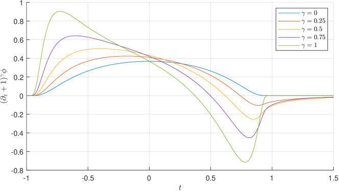
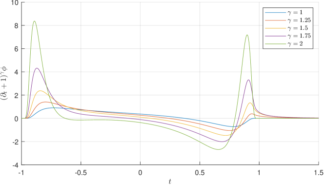
Figure 1. Graphs of the fractional parabolic derivative $(\partial_{t}+1)^{\gamma}\phi$ with $\phi$ from (4.57) for certain values of $\gamma\in[0,2]$. Note the different scales on the $y$-axes.

Note the contrast with the merely spatial Matérn case, where the self-adjointness of the shifted Laplacian $\kappa^{2}-\Delta$ causes $L_{\beta}^{*}L_{\beta}=\tau^{2}(\kappa^{2}-\Delta)^{2\beta}$, thus we find a weak Markov property also for half-integer values of $\beta\in(0,\infty)$.

5. Fractional $Q$-Wiener process

In this section we consider the fractional $Q$-Wiener process, which is a $U$-valued analog to fractional Brownian motion; we define it as in [12, Definition 2.1].

Definition 5.1.

Let $Q\in\mathscr{L}_{1}^{+}(U)$. A $U$-valued Gaussian process $(W^{Q}_{H}(t))_{t\in\mathbb{R}}$ is called a fractional $Q$-Wiener process with Hurst parameter $H\in(0,1)$ if

1. $\mathbb{E}[W^{Q}_{H}(t)]=0$ for all $t\in\mathbb{R}$;

2. $Q_{H}(s,t)=\frac{1}{2}(|t|^{2H}+|s|^{2H}-|t-s|^{2H})Q$ for all $s,t\in\mathbb{R}$;

3. $W^{Q}_{H}$ has continuous sample paths.

Here, $(Q_{H}(s,t))_{s,t\in\mathbb{R}}\subseteq\mathscr{L}_{1}^{+}(U)$ are the covariance operators of $W^{Q}_{H}$, cf. (4.17).

Note that for $H=\frac{1}{2}$, the above definition reduces to a characterization of a standard (non-fractional) $Q$-Wiener process when restricted to $[0,\infty)$.

In the real-valued setting, the fractional Brownian motion can also be represented as a stochastic integral over $\mathbb{R}$ [31, Definition 2.1]. Proposition 5.2 below shows that such a representation is also available in the $U$-valued setting using the stochastic integral over $\mathbb{R}$ from Section 2.2. This representation can be leveraged to prove that a fractional $Q$-Wiener process can be viewed as a limiting case of the class of processes discussed in Section 4, see Proposition 5.3. We conclude this section by making some remarks about the Markov behavior of $W^{Q}_{H}$, see Subsection 5.2.

5.1. Integral representation and relation to $Z_{\gamma}$

Let $Q\in\mathscr{L}_{1}^{+}(U)$ and let $(W^{Q}(t))_{t\in\mathbb{R}}$ be a two-sided $Q$-Wiener process, see Subsection 2.2. We define the process $(\widehat{W}^{Q}_{H}(t))_{t\in\mathbb{R}}$ via the following Mandelbrot–Van Ness [31] type integral:

$$\widehat{W}_{H}^{Q}(t):=\int_{\mathbb{R}}K_{H}(t,r)\mathop{}\!\mathrm{d}W^{Q}(r),\quad t\in\mathbb{R},$$ (5.1)

where the integration kernel $K_{H}\colon\mathbb{R}^{2}\to\mathbb{R}$ given by

$$K_{H}(t,r):=\frac{(t-r)^{H-\frac{1}{2}}_{+}-(-r)_{+}^{H-\frac{1}{2}}}{C_{H}},\quad(t,r)\in\mathbb{R}^{2}.$$ (5.2)

The normalizing constant $C_{H}$ is chosen as

$$C_{H}:=\int_{\mathbb{R}}\Bigl{|}(1-r)_{+}^{H-\frac{1}{2}}-(-r)^{H-\frac{1}{2}}_{+}\Bigr{|}^{2}\mathop{}\!\mathrm{d}r=\frac{3-2H}{4H}\mathrm{B}(2-2H,H+\tfrac{1}{2}),$$

where $\mathrm{B}$ denotes the beta function [39, Theorem B.1], so that $\widehat{Q}_{H}(1,1)=Q$, where $(\widehat{Q}_{H}(t,s))_{t,s\in\mathbb{R}}$ denotes the family of covariance operators associated to $\widehat{W}^{Q}_{H}$. From this definition it follows that

$$\widehat{W}^{Q}_{H}(t)=\frac{1}{C_{H}}\int_{-\infty}^{0}[(t-r)^{H-\frac{1}{2}}-(-r)^{H-\frac{1}{2}}]\mathop{}\!\mathrm{d}W^{Q}(r)+\frac{1}{C_{H}}\int_{0}^{t}(t-r)^{H-\frac{1}{2}}\mathop{}\!\mathrm{d}W^{Q}(r)$$ (5.3)

for $t\in[0,\infty)$, whereas for $t\in(-\infty,0)$ we have

$$\widehat{W}^{Q}_{H}(t)=\frac{1}{C_{H}}\int_{-\infty}^{t}[(t-r)^{H-\frac{1}{2}}-(-r)^{H-\frac{1}{2}}]\mathop{}\!\mathrm{d}W^{Q}(r)+\frac{1}{C_{H}}\int_{t}^{0}(-r)^{H-\frac{1}{2}}\mathop{}\!\mathrm{d}W^{Q}(r).$$ (5.4)

In particular, for $H=\frac{1}{2}$ and $t\in[0,\infty)$ we find $\widehat{W}^{Q}_{\nicefrac{{1}}{{2}}}(t)=W^{Q}(t)$, $\mathbb{P}$-a.s.

We then have the following relation to the fractional $Q$-Wiener process:

Proposition 5.2.

Formula (5.1) yields a well-defined square-integrable random variable $\widehat{W}^{Q}_{H}(t)\in L^{2}(\Omega,\mathcal{F}_{t}^{\delta W^{Q}},\mathbb{P};U)$ for each $t\in\mathbb{R}$, and there exists a modification of the process $(\widehat{W}^{Q}_{H}(t))_{t\in\mathbb{R}}$ which is a fractional $Q$-Wiener process in the sense of Definition 5.1.

Proof.

By the Itô isometry (2.2) it suffices to note that

$$\mathbb{E}\Bigl{[}\bigl{\|}\widehat{W}^{Q}_{H}(t)\bigr{\|}_{U}^{2}\Bigr{]}=\int_{\mathbb{R}}\|K_{H}(t,r)Q^{\frac{1}{2}}\|_{\mathscr{L}_{2}(U)}^{2}\mathop{}\!\mathrm{d}r=\operatorname{tr}Q\int_{\mathbb{R}}|K_{H}(t,r)|^{2}\mathop{}\!\mathrm{d}r<\infty$$

to see that $\widehat{W}^{Q}_{H}(t)\in L^{2}(\Omega;U)$ is well-defined. Since $K_{H}$ is a deterministic kernel integrated with respect to a mean-zero Gaussian process $W^{Q}$, it readily follows that $\widehat{W}^{Q}_{H}$ is also mean-zero Gaussian. For the covariance operators $(\widehat{Q}_{H}(t,s))_{t,s\in\mathbb{R}}$ of $\widehat{W}^{Q}_{H}$, we can argue as in the proof of Proposition 4.7 to find

$$\forall t,s\in\mathbb{R}:\quad\widehat{Q}_{H}(t,s)=\int_{\mathbb{R}}K_{H}(s,r)K_{H}(t,r)\mathop{}\!\mathrm{d}r\,Q=\mathbb{E}[B_{H}(t)B_{H}(s)]\,Q,$$ (5.5)

where $B_{H}=(B_{H}(t))_{t\in\mathbb{R}}$ denotes (real-valued) fractional Brownian motion. Hence (f-WP2) holds by the properties of $B_{H}$.

Lastly, we shall establish the existence of a continuous modification of (5.1). To this end, we first remark that $\widehat{W}^{Q}_{H}$ is self-similar with exponent $H$ and that its increments are stationary; this means for any $t\in\mathbb{R}$ we have, respectively,

$$\forall\alpha\in(0,\infty) :\quad\widehat{W}^{Q}_{H}(\alpha t)\overset{d}{=}\alpha^{H}\widehat{W}^{Q}_{H}(t),$$ (5.6)

$$\forall h\in\mathbb{R} :\quad\widehat{W}^{Q}_{H}(t+h)-\widehat{W}^{Q}_{H}(t)\overset{d}{=}\widehat{W}^{Q}_{H}(h).$$ (5.7)

The proofs of these statements are analogous to the real-valued case; they involve changing variables in the integral (5.1) and using the facts that $\alpha^{-\frac{1}{2}}W^{Q}(\alpha\,\cdot\,)$ and $W^{Q}(\,\cdot\,+h)$, respectively, are also two-sided $Q$-Wiener processes. Thus,

$$\bigl{\|}\widehat{W}^{Q}_{H}(t+h)-\widehat{W}^{Q}_{H}(t)\bigr{\|}_{L^{p}(\Omega;U)}=\bigl{\|}\widehat{W}^{Q}_{H}(|h|)\bigr{\|}_{L^{p}(\Omega;U)}=|h|^{H}\bigl{\|}\widehat{W}^{Q}_{H}(1)\bigr{\|}_{L^{p}(\Omega;U)}$$ (5.8)

for any $p\in(1,\infty)$. By the Kahane–Khintchine inequalities (see, e.g., [20, Theorem 6.2.6]), there exists a constant $C_{p}\in(0,\infty)$ such that

$$\bigl{\|}\widehat{W}^{Q}_{H}(1)\bigr{\|}_{L^{p}(\Omega;U)}\leq C_{p}\bigl{\|}\widehat{W}^{Q}_{H}(1)\bigr{\|}_{L^{2}(\Omega;U)}=C_{p}\operatorname{tr}Q.$$

We have thus shown that $t\mapsto\widehat{W}^{Q}_{H}(t)$ is $H$-Hölder continuous from $\mathbb{R}$ to $L^{p}(\Omega;U)$. Since $p\in(1,\infty)$ was arbitrary, we can apply the Kolmogorov–Chentsov theorem [8, Corollary 3.10] with $p\in(\nicefrac{{1}}{{H}},\infty)$ to conclude that $\widehat{W}^{Q}_{H}$ has a modification with continuous sample paths. ∎

Now we consider the relation between fractional $Q$-Wiener process and the process $Z_{\gamma}$ considered in Section 4. For $\varepsilon\in(0,\infty)$, let $Z_{\gamma}^{\varepsilon}$ denote the mild solution to (4.1) with $A=\varepsilon\operatorname{Id}_{U}$ and define the process $\bigl{(}\overline{Z}_{\gamma}^{\varepsilon}(t)\bigr{)}_{t\in\mathbb{R}}$ by

$$\overline{Z}_{\gamma}^{\varepsilon}(t):=\frac{\Gamma(\gamma)}{C_{\gamma-\frac{1}{2}}}(Z_{\gamma}^{\varepsilon}(t)-Z_{\gamma}^{\varepsilon}(0)),\quad t\in\mathbb{R}.$$ (5.9)

Note that $\widehat{W}^{Q}_{H}(t)$ can formally be written as a “convergent difference of divergent integrals,” cf. [31, Footnote 3]:

$$\frac{1}{C_{H}}\biggl{[}\int_{-\infty}^{t}(t-s)^{H-\frac{1}{2}}\mathop{}\!\mathrm{d}W^{Q}(s)-\int_{-\infty}^{0}(-s)^{H-\frac{1}{2}}\mathop{}\!\mathrm{d}W^{Q}(s)\biggr{]}.$$

The above expression would correspond to taking $\varepsilon=0$ in (5.9), which is ill-defined since Assumption 4.2(i) cannot be satisfied. However, the next result shows that a fractional $Q$-Wiener process can be viewed as a limiting case of $\overline{Z}_{\gamma}^{\varepsilon}$ as $\varepsilon\downarrow 0$.

Proposition 5.3.

Let $Q\in\mathscr{L}_{1}^{+}(U)$ and $\gamma\in(\nicefrac{{1}}{{2}},\nicefrac{{3}}{{2}})$. The family of stochastic processes $(\overline{Z}_{\gamma}^{\varepsilon})_{\varepsilon\in(0,\infty)}$ defined by (5.9) converges uniformly on compact subsets of $\mathbb{R}$ in mean-square sense to the fractional $Q$-Wiener process $\widehat{W}^{Q}_{H}$ in (5.1) with Hurst parameter $H=\gamma-\frac{1}{2}$ as $\varepsilon\downarrow 0$:

$$\forall\,T\in(0,\infty):\quad\lim_{\varepsilon\downarrow 0}\sup_{t\in[-T,T]}\left\|\widehat{W}^{Q}_{\gamma-\frac{1}{2}}(t)-\overline{Z}_{\gamma}^{\varepsilon}(t)\right\|_{L^{2}(\Omega;U)}=0.$$ (5.10)

Proof.

For $t\in[0,\infty)$, we can write

$$\widehat{W}^{Q}_{\gamma-\frac{1}{2}}(t) -\overline{Z}_{\gamma}^{\varepsilon}(t)=\frac{1}{C_{\gamma-\frac{1}{2}}}\int_{0}^{t}(t-s)^{\gamma-1}\bigl{(}1-e^{-\varepsilon(t-s)}\bigr{)}\mathop{}\!\mathrm{d}W^{Q}(s)$$

$$+\frac{1}{C_{\gamma-\frac{1}{2}}}\int_{-\infty}^{0}\left[(t-s)^{\gamma-1}\bigl{(}1-e^{-\varepsilon(t-s)}\bigr{)}-(-s)^{\gamma-1}\bigl{(}1-e^{\varepsilon s}\bigr{)}\right]\mathop{}\!\mathrm{d}W^{Q}(s).$$

After applying the Itô isometry to each of these integrals and using the respective changes of variables $s^{\prime}:=-s$ and $s^{\prime}:=t-s$, we obtain

$$\biggl{\|}\widehat{W}^{Q}_{\gamma-\frac{1}{2}}(t) -\overline{Z}_{\gamma}^{\varepsilon}(t)\biggr{\|}_{L^{2}(\Omega;U)}^{2}=\frac{I_{1}(t)+I_{2}(t)}{C_{\gamma-\frac{1}{2}}}(\operatorname{tr}Q)^{2},$$ (5.11)

$$I_{1}(t) :=\int_{0}^{|t|}s^{2\gamma-2}\bigl{(}1-e^{-\varepsilon s}\bigr{)}^{2}\mathop{}\!\mathrm{d}s,$$ (5.12)

$$I_{2}(t) :=\int_{0}^{\infty}\left|(|t|+s)^{\gamma-1}\bigl{(}1-e^{-\varepsilon(|t|+s)}\bigr{)}-s^{\gamma-1}\bigl{(}1-e^{-\varepsilon s}\bigr{)}\right|^{2}\mathop{}\!\mathrm{d}s.$$ (5.13)

For $t\in(-\infty,0)$ we find (5.11) by instead splitting into integrals over $(-\infty,t)$ and $(t,0)$ and changing variables $s^{\prime}:=t-s$ and $s^{\prime}:=-s$, respectively.

For $t\in[-T,T]$, the estimate $1-e^{-x}\leq x$ for $x\in[0,\infty)$ yields for the first term:

$$I_{1}(t)\leq\varepsilon^{2}\int_{0}^{\lvert t\rvert}s^{2\gamma}\mathop{}\!\mathrm{d}s=\frac{\varepsilon^{2}\lvert t\rvert^{2\gamma+1}}{2\gamma+1}\leq\frac{\varepsilon^{2}T^{2\gamma+1}}{2\gamma+1}.$$

For $I_{2}$, we apply the fundamental theorem of calculus to the function

$$u\mapsto(u+s)^{\gamma-1}(1-e^{-\varepsilon(u+s)}),$$

followed by Minkowski’s integral inequality [44, Section A.1] to find

$$I_{2} (t)=\int_{0}^{\infty}\biggl{|}\int_{0}^{\lvert t\rvert}[(\gamma-1)(u+s)^{\gamma-2}(1-e^{-\varepsilon(u+s)})+\varepsilon(u+s)^{\gamma-1}e^{-\varepsilon(u+s)}]\mathop{}\!\mathrm{d}u\biggr{|}^{2}\mathop{}\!\mathrm{d}s$$

$$\leq\Biggl{(}\int_{0}^{T}\biggl{[}\int_{0}^{\infty}\Bigl{|}(\gamma-1)(u+s)^{\gamma-2}(1-e^{-\varepsilon(u+s)})+\varepsilon(u+s)^{\gamma-1}e^{-\varepsilon(u+s)}\Bigr{|}^{2}\mathop{}\!\mathrm{d}s\biggr{]}^{\frac{1}{2}}\mathop{}\!\mathrm{d}u\Biggr{)}^{2}$$

$$=\varepsilon^{3-2\gamma}\Biggl{(}\int_{0}^{T}\biggl{[}\int_{\varepsilon u}^{\infty}\Bigl{|}(\gamma-1)v^{\gamma-2}(1-e^{-v})+v^{\gamma-1}e^{-v}\Bigr{|}^{2}\mathop{}\!\mathrm{d}v\biggr{]}^{\frac{1}{2}}\mathop{}\!\mathrm{d}u\Biggr{)}^{2}$$

$$\leq\varepsilon^{3-2\gamma}\,T^{2}\int_{0}^{\infty}\Bigl{|}(\gamma-1)v^{\gamma-2}(1-e^{-v})+v^{\gamma-1}e^{-v}\Bigr{|}^{2}\mathop{}\!\mathrm{d}v,$$

where we performed the change of variables $v(s):=\varepsilon(u+s)$ on the third line.

The improper integral on the last line converges: As $v\downarrow 0$, the squares of both terms are of order $\mathcal{O}(v^{2\gamma-2})$, where we again use $1-e^{-v}\leq v$ for the first term, and we have $2\gamma-2\in(-1,1)$; the square of the first term is of order $\mathcal{O}(v^{2\gamma-4})$ as $v\to\infty$, with $2\gamma-4\in(-3,-1)$, whereas the second term decays exponentially.

The convergence thus follows by letting $\varepsilon\downarrow 0$ in the previous two displays. ∎

5.2. Remarks on Markov behavior

Now we consider the Markov behavior of fractional $Q$-Wiener processes with Hurst parameter $H\in(0,1)$. Since the case $H=\frac{1}{2}$ corresponds to a standard $Q$-Wiener process, we find that $W^{Q}_{\nicefrac{{1}}{{2}}}$ is simple Markov, whereas we can expect that $W^{Q}_{H}$ is not weakly Markov for $H\neq\frac{1}{2}$.

In the real-valued case, the first published proof of non-Markovianity appears to be [19], which shows that $B_{H}$ is not simple Markov for $H\neq\frac{1}{2}$ using a characterization in terms of its covariance function which is valid for Gaussian processes. This result can be improved by applying the theory of [18, Chapter V] for Gaussian $N$-ple Markov processes to the Mandelbrot–Van Ness representation of $B_{H}$. Namely, according to [18, Theorem 5.1], any real-valued Gaussian process of the form

$$\biggl{(}\int_{-\infty}^{t}K(t,s)\mathop{}\!\mathrm{d}B(s)\biggr{)}_{t\in\mathbb{R}}$$

can only be $N$-ple Markov for $N\in\mathbb{N}$ if its integration kernel $F$ can be written as

$$K(s,t)=\sum_{j=1}^{N}f_{j}(s)g_{j}(t)$$

for some functions $(f_{j})_{j=1}^{N},(g_{j})_{j=1}^{N}$. This condition is not satisfied for $K_{H}$ from (5.2).

In order to establish that $W^{Q}_{H}$ (or $B_{H}$) does not have the weak Markov property for $H\neq\frac{1}{2}$, one could attempt to associate a nonlocal precision operator to the process and apply the necessary condition from Theorem 3.8. Formally, the coloring operator $\mathcal{L}^{-1}_{H}$ of $W^{Q}_{H}$ acts on functions $f\colon\mathbb{R}\to U$ as

$$\mathcal{L}^{-1}_{H}f(t)=\frac{1}{C_{H}}\int_{\mathbb{R}}K_{H}(t,s)f(s)\mathop{}\!\mathrm{d}s,\quad\forall t\in\mathbb{R}.$$

For certain ranges of $H$, see for instance [39, Equation (31)], an explicit formula of its inverse $\mathcal{L}_{H}$ can also be determined. The operator $\mathcal{L}^{-1}_{H}$ is bounded on some weighted Hölder space by [39, Theorem 6], but there is no reason to expect that it is bounded on a Hilbert space such as $L^{2}(\mathbb{R};U)$. Therefore, Theorem 3.8 is not directly applicable, as it would need to be extended to the Banach space setting, which is beyond the scope of this work.

Funding

K.K. acknowledges support of the research project Efficient spatiotemporal statistical modelling with stochastic PDEs (with project number VI.Veni.212.021) by the talent programme Veni which is financed by the Dutch Research Council (NWO).

Appendix A Spaces of vector-valued functions

A.1. Spaces of measurable, continuous and differentiable functions

Let $(S,\mathscr{A},\mu)$ be a measure space. We abbreviate the phrases “almost everywhere” and “almost all” by “a.e.” and “a.a.”​, respectively.

Let $\mathcal{B}(E)$ denote the Borel $\sigma$-algebra of $E$. Given $x\in E$ and $f\colon S\to\mathbb{R}$, we define $f\otimes x\colon S\to E$ by $[f\otimes x](\,\cdot\,):=f(\,\cdot\,)x$. A function $f\colon(S,\mathscr{A},\mu)\to(E,\mathcal{B}(E))$ is said to be $\mu$-strongly measurable if it is the $\mu$-a.e. limit of linear combinations of $\mathbf{1}_{A}\otimes x$, where $x\in E$ and $A\in\mathscr{A}$ with $\mu(A)<\infty$. We denote by $B_{b}(S,\mathscr{A})$ (resp. $C_{b}(S)$) the Banach space of $\mathscr{A}$-measurable (resp. continuous) and bounded functions $f\colon S\to\mathbb{R}$ endowed with the norm $\|f\|_{B_{b}(S,\mathscr{A})}=\|f\|_{C_{b}(S)}=\sup_{s\in S}|f(s)|$. If the $\sigma$-algebra is clear from context, we may simply write $B_{b}(S)$. The set $C_{c}^{\infty}(J;E)$ consists of infinitely differentiable functions from $J$ to $E$ with compact support.

A.2. Bochner and Sobolev spaces

For $p\in[1,\infty)$, let $L^{p}(S,\mathscr{A}\!,\mu;E)$ denote the Bochner space of (equivalence classes of) strongly measurable, $p$-integrable functions equipped with the norm $\|f\|_{L^{p}(S,\mathscr{A}\!,\mu;E)}:=\left(\int_{S}\|f(s)\|_{E}^{p}\mathop{}\!\mathrm{d}\mu(s)\right)^{\!\nicefrac{{1}}{{p}}}\!\!.$ If the $\sigma$-algebra and measure are clear from context, we may suppress them from our notation and simply write $L^{p}(S;E)$. The space $L^{2}(S,\mathscr{A}\!,\mu;U)$ is a Hilbert space when equipped with the inner product $\langle f,g\rangle_{L^{2}(S,\mathscr{A}\!,\mu;U)}:=\int_{S}\langle f(s),g(s)\rangle_{U}\mathop{}\!\mathrm{d}\mu(s)$.

If $(S,\mathscr{A}\!,\mu)$ and $(T,\mathscr{B},\nu)$ are $\sigma$-finite measure spaces, then the measurable space $(S\times T,\mathscr{A}\otimes\mathscr{B})$, equipped with the product $\sigma$-algebra

$$\mathscr{A}\otimes\mathscr{B}:=\sigma(A\times B:A\in\mathscr{A},B\in\mathscr{B}),$$

admits a unique $\sigma$-finite product measure $\mu\times\nu$ satisfying

$$(\mu\times\nu)(A\times B)=\mu(A)\nu(B)\quad\forall A\in\mathscr{A},\,B\in\mathscr{B}.$$

For $p,q\in[1,\infty)$, we define the mixed-exponent Bochner space $L^{p,q}(S\times T;E)$ as the Banach space of (equivalence classes of) strongly $(\mu\times\nu)$-measurable functions $f\colon S\times T\to E$ such that

$$\|f\|_{L^{p,q}(S\times T;E)}:=\biggl{[}\int_{S}\biggl{[}\int_{T}\|f(s,t)\|_{E}^{q}\mathop{}\!\mathrm{d}\nu(t)\biggr{]}^{\frac{p}{q}}\mathop{}\!\mathrm{d}\mu(s)\biggr{]}^{\frac{1}{p}}<\infty.$$ (A.1)

Intervals $J\subseteq\mathbb{R}$ will be equipped with the Lebesgue measure $\lambda$ and Lebesgue $\sigma$-algebra $\mathcal{B}(J)\vee\sigma(\mathcal{N}_{\lambda})$. A function $f\in L^{p}(J;E)$ is said to be weakly differentiable, with weak derivative $\partial_{t}f$, if

$$\int_{J}\phi^{\prime}(t)f(t)\mathop{}\!\mathrm{d}t=-\int_{J}\phi(t)[\partial_{t}f](t)\mathop{}\!\mathrm{d}t\quad\forall\phi\in C^{\infty}_{c}(J;\mathbb{R}).$$

More generally, we denote its $n$th weak derivative by $\partial_{t}^{n}f$. If $\partial_{t}^{\,j}f\in L^{p}(J;E)$ for all $j\in\{0,\dots,n\}$, then $f$ belongs to the Bochner–Sobolev space $W^{n,p}(J;E)$, which is a Banach space using the norm $\|f\|_{W^{n,p}(J;E)}:=(\sum_{j=0}^{n}\|\partial_{t}^{j}f\|_{L^{p}(J;E)}^{p})^{\nicefrac{{1}}{{p}}}$. If $p=2$ and $E=U$, then $H^{n}(J;U):=W^{n,2}(J;U)$ is a Hilbert space whose norm is induced by the inner product $\langle f,g\rangle_{H^{n}(J;U)}:=\sum_{j=0}^{n}\langle\partial_{t}^{\,j}f,\partial_{t}^{\,j}g\rangle_{L^{2}(J;U)}$.

Appendix B Auxiliary results

This appendix collects some auxiliary results which are needed in the main text but have been postponed for the sake of readability.

B.1. Facts regarding conditional independence

Let $\mathcal{G}_{1},\mathcal{H},\mathcal{G}_{2}\subseteq\mathcal{F}$ be $\sigma$-algebras on $(\Omega,\mathcal{F},\mathbb{P})$. We recall a characterization of conditional independence, see [21, Theorem 8.9], from which we derive a lemma which is useful for establishing relations between various (equivalent formulations of) Markov properties defined in Section 3.

Theorem B.1 (Doob’s conditional independence property).

We have $\mathcal{G}_{1}\perp\!\!\!\perp_{\mathcal{H}}\mathcal{G}_{2}$ if and only if

$$\mathbb{P}(G_{2}\mid\mathcal{G}_{1}\vee\mathcal{H})=\mathbb{P}(G_{2}\mid\mathcal{H}),\quad\mathbb{P}\text{-a.s.},\quad\forall G_{2}\in\mathcal{G}_{2}.$$ (B.1)

Lemma B.2.

If $\mathcal{G}_{1}\perp\!\!\!\perp_{\mathcal{H}}\mathcal{G}_{2}$, then

1. $\mathcal{G}_{1}\vee\mathcal{H}\perp\!\!\!\perp_{\mathcal{H}}\mathcal{G}_{2}$;

2. $\mathcal{G}_{1}\perp\!\!\!\perp_{\mathcal{H}^{\prime}}\mathcal{G}_{2}$ for any $\sigma$-algebra $\mathcal{H}^{\prime}\supseteq\mathcal{H}$ such that $\mathcal{H}^{\prime}\subseteq\mathcal{G}_{1}$;

3. $\mathcal{G}_{1}\perp\!\!\!\perp_{\mathcal{H}^{\prime}}\mathcal{G}_{2}$ for any $\sigma$-algebra $\mathcal{H}^{\prime}\supseteq\mathcal{H}$ of the form $\mathcal{H}^{\prime}=\mathcal{H}^{\prime}_{1}\vee\mathcal{H}_{2}^{\prime},$ where $\mathcal{H}^{\prime}_{1},\mathcal{H}^{\prime}_{2}$ are $\sigma$-algebras satisfying $\mathcal{H}_{1}^{\prime}\subseteq\mathcal{G}_{1}\vee\mathcal{H}$ and $\mathcal{H}_{2}^{\prime}\subseteq\mathcal{G}_{2}\vee\mathcal{H}$.

Proof.

Part a is [21, Corollary 8.11(i)]; combining it with $\mathcal{G}_{1}=\mathcal{G}_{1}\vee\mathcal{H}^{\prime}$ and ${\mathcal{H}^{\prime}=\mathcal{H}\vee\mathcal{H}^{\prime}}$ yields b. To prove (c), first note that $\mathcal{G}_{1}\vee\mathcal{H}\perp\!\!\!\perp_{\mathcal{H}\vee\mathcal{H}_{1}^{\prime}}\mathcal{G}_{2}\vee\mathcal{H}$ by parts a and b. Applying a again, we find

$$\mathcal{G}_{1}\vee\mathcal{H}\vee\mathcal{H}_{1}^{\prime}\perp\!\!\!\perp_{\mathcal{H}\vee\mathcal{H}_{1}^{\prime}}\mathcal{G}_{2}\vee\mathcal{H}\vee\mathcal{H}_{1}^{\prime}.$$

Since $\mathcal{H}\vee\mathcal{H}_{1}^{\prime}\subseteq\mathcal{H}\vee\mathcal{H}^{\prime}=\mathcal{H}^{\prime}=\mathcal{H}_{2}^{\prime}\vee\mathcal{H}_{1}^{\prime}\subseteq\mathcal{G}_{2}\vee\mathcal{H}\vee\mathcal{H}_{1}^{\prime}$, part b yields

$$\mathcal{G}_{1}\vee\mathcal{H}\vee\mathcal{H}_{1}^{\prime}\perp\!\!\!\perp_{\mathcal{H}^{\prime}}\mathcal{G}_{2}\vee\mathcal{H}\vee\mathcal{H}_{1}^{\prime},$$

which proves c since $\mathcal{G}_{1}\subseteq\mathcal{G}_{1}\vee\mathcal{H}\vee\mathcal{H}_{1}^{\prime}$ and $\mathcal{G}_{2}\subseteq\mathcal{G}_{2}\vee\mathcal{H}\vee\mathcal{H}_{1}^{\prime}$. ∎

B.2. Facts regarding Assumption 4.2(i)

Lemma B.3.

Let Assumption 4.1 be satisfied, i.e., suppose the linear operator $-A\colon\mathsf{D}(A)\subseteq U\to U$ on the separable real Hilbert space $U$ generates an exponentially stable $C_{0}$-semigroup $(S(t))_{t\geq 0}$ of bounded linear operators on $U$. If $Q\in\mathscr{L}^{+}(U)$ and $\gamma_{0}\in(-\infty,\nicefrac{{1}}{{2}}]$, then

$$\int_{0}^{\infty}\|t^{\gamma_{0}-1}S(t)Q^{\frac{1}{2}}\|_{\mathscr{L}_{2}(U)}^{2}\mathop{}\!\mathrm{d}t=\infty,$$

that is, Assumption 4.2(i) cannot hold for $\gamma_{0}\in(-\infty,\nicefrac{{1}}{{2}}]$.

Proof.

Fix some $x\in U$ with $\|x\|_{U}=1$. Then $\|S(t)Q^{\frac{1}{2}}\|_{\mathscr{L}_{2}(U)}\geq\|S(t)Q^{\frac{1}{2}}x\|_{U}$ for all $t\in[0,\infty)$. Since $t\mapsto S(t)Q^{\frac{1}{2}}x$ is continuous at zero and $S(0)Q^{\frac{1}{2}}x=Q^{\frac{1}{2}}x$, we can choose $\delta\in(0,\infty)$ so small that $\|S(t)Q^{\frac{1}{2}}x\|_{U}\geq\frac{1}{2}\|Q^{\frac{1}{2}}x\|_{U}$ for all $t\in[0,\delta]$. If $\gamma_{0}\in(-\infty,\nicefrac{{1}}{{2}}]$, we then obtain

$$\int_{0}^{\infty}\|t^{\gamma_{0}-1}S(t)Q^{\frac{1}{2}}\|_{\mathscr{L}_{2}(U)}^{2}\mathop{}\!\mathrm{d}t\geq\frac{1}{2}\|Q^{\frac{1}{2}}x\|_{U}\int_{0}^{\delta}t^{2(\gamma_{0}-1)}\mathop{}\!\mathrm{d}t=\infty.\qed$$

Lemma B.4.

Let Assumption 4.1 be satisfied. If Assumptions 4.2(i) holds for some $\gamma_{0}\in(\nicefrac{{1}}{{2}},\infty)$, then it also holds for all $\gamma^{\prime}\in[\gamma_{0},\infty)$.

Proof.

The change of variables $\tau:=t/2$, the semigroup property and (4.2) yield

$$\int_{0}^{\infty}\|t^{\gamma^{\prime}-1}S(t)Q^{\frac{1}{2}}\|_{\mathscr{L}_{2}(U)}^{2}\mathop{}\!\mathrm{d}t \leq 2^{2\gamma^{\prime}-1}M_{0}^{2}\int_{0}^{\infty}e^{-2w\tau}\|\tau^{\gamma^{\prime}-1}S(\tau)Q^{\frac{1}{2}}\|_{\mathscr{L}_{2}(U)}^{2}\mathop{}\!\mathrm{d}\tau.$$

For the latter integral, we split up the domain of integration and estimate each of the resulting integrands to find

$$\int_{0}^{\infty} e^{-2w\tau}\|\tau^{\gamma^{\prime}-1}S(\tau)Q^{\frac{1}{2}}\|_{\mathscr{L}_{2}(U)}^{2}\mathop{}\!\mathrm{d}\tau=\sum_{k=1}^{\infty}\int_{k-1}^{k}e^{-2w\tau}\|\tau^{\gamma^{\prime}-1}S(\tau)Q^{\frac{1}{2}}\|_{\mathscr{L}_{2}(U)}^{2}\mathop{}\!\mathrm{d}\tau$$

$$\leq\sum_{k=1}^{\infty}e^{-2w(k-1)}k^{2(\gamma^{\prime}-\gamma_{0})}\int_{0}^{\infty}\|\tau^{\gamma_{0}-1}S(\tau)Q^{\frac{1}{2}}\|_{\mathscr{L}_{2}(U)}^{2}\mathop{}\!\mathrm{d}\tau<\infty,$$

where the series converges since $|e^{-2wk}k^{2(\gamma^{\prime}-\gamma_{0})}|^{\frac{1}{k}}\to e^{-2w}<1$ as $k\to\infty$. ∎

B.3. Filtrations indexed by the real line

The proof of Proposition B.6 below elaborates on [2, Example 3.6]. First we state and prove a lemma which shows that collections of random variables are generated by a $\pi$-system consisting of finite products of bounded, real-valued random variables.

Lemma B.5.

If $(X_{i})_{i\in\mathcal{I}}$ is a collection of $U$-valued random variables, then

$$\sigma(X_{i}:i\in\mathcal{I})=\sigma\left(\prod\nolimits_{i\in\mathcal{J}}Z_{i}:\mathcal{J}\subseteq\mathcal{I}\textup{ finite},\,Z_{i}\in B_{b}(\Omega,\sigma(X_{i})),\forall i\in\mathcal{J}\!\right)\!.$$ (B.2)

Proof.

The “$\supseteq$” inclusion holds because any $Z=\prod_{i\in\mathcal{J}}Z_{i}$ is measurable with respect to $\bigvee_{i\in\mathcal{J}}\sigma(X_{i})\subseteq\bigvee_{i\in\mathcal{I}}\sigma(X_{i})$ for any $\mathcal{J}\subseteq\mathcal{I}$. For the converse inclusion, note that the join of a family of $\sigma$-algebras $(\mathcal{A}_{i})_{i\in\mathcal{I}}$ has the following general property:

$$\bigvee_{i\in\mathcal{I}}\mathcal{A}_{i}=\sigma\left(\bigcap\nolimits_{i\in\mathcal{J}}A_{i}:\mathcal{J}\subseteq\mathcal{I}\text{ finite},\,A_{i}\in\mathcal{A}_{i}\,\,\forall i\in\mathcal{J}\right)\!.$$

Thus, by definition of $\sigma(X_{i})$, we obtain (see also [40, Chapter 0, Theorem 2.3])

$$\sigma(X_{i}:i\in\mathcal{I})=\sigma\left(\bigcap\nolimits_{i\in\mathcal{J}}X_{i}^{-1}[B_{i}]:\mathcal{J}\subseteq\mathcal{I}\text{ finite},\,B_{i}\in\mathcal{B}(U)\,\,\forall i\in\mathcal{J}\right)\!.$$ (B.3)

Since $\bigcap_{i\in\mathcal{J}}X_{i}^{-1}[B_{i}]=(\prod_{i\in\mathcal{J}}\mathbf{1}_{B_{i}}(X_{i}))^{-1}[\{1\}]$ for any finite $\{B_{i}:i\in\mathcal{J}\}\subseteq\mathcal{B}(U)$, we find that the right-hand side of (B.3) is contained in that of (B.2). ∎

Proposition B.6.

Let $(W^{Q}(t))_{t\in\mathbb{R}}$ be a $U$-valued two-sided $Q$-Wiener process with covariance operator $Q\in\mathscr{L}_{1}^{+}(U)$, see Subsection 2.2. The filtration $(\mathcal{F}^{\delta W^{Q}}_{t})_{t\in\mathbb{R}}$ defined in (2.3) is right-continuous, i.e., we have $\mathcal{F}_{t+}^{\delta W^{Q}}:=\bigcap_{\varepsilon>0}\mathcal{F}_{t+\varepsilon}^{\delta W^{Q}}=\mathcal{F}_{t}^{\delta W^{Q}}$ for all $t\in\mathbb{R}$.

Proof.

Fix $t\in\mathbb{R}$. It suffices to prove that

$$\mathbb{E}[Z\mid\mathcal{F}^{\delta W^{Q}}_{t+}]=\mathbb{E}[Z\mid\mathcal{F}^{\delta W^{Q}}_{t}],\quad\mathbb{P}\text{-a.s.},$$ (B.4)

for all $Z\in B_{b}(\Omega,\mathcal{F}_{\infty}^{\delta W^{Q}})$, where $\mathcal{F}_{\infty}^{\delta W^{Q}}:=\sigma(W_{s,u}:s\leq u)$, using the shorthand notation $W_{s,u}=W^{Q}(u)-W^{Q}(s)$. Indeed, given $A\in\mathcal{F}_{t+}^{\delta W^{Q}}\subseteq\mathcal{F}_{\infty}^{\delta W^{Q}}$, equation (B.4) would imply that $\mathbf{1}_{A}$ is $\mathbb{P}$-a.s. equal to the $\mathcal{F}_{t}^{\delta W^{Q}}$-measurable random variable $\mathbb{E}[\mathbf{1}_{A}\mid\mathcal{F}^{\delta W^{Q}}_{t}]$, and thus $A\in\mathcal{F}_{t}^{\delta W^{Q}}$ by the completeness of $(\mathcal{F}_{t}^{\delta W^{Q}})_{t\in\mathbb{R}}$. This yields $\mathcal{F}_{t+}^{\delta W^{Q}}\subseteq\mathcal{F}_{t}^{\delta W^{Q}}$​.

Let $\mathscr{H}$ denote the linear space of bounded random variables $Z\colon\Omega\to\mathbb{R}$ for which (B.4) holds; we want to show that $B_{b}(\Omega,\mathcal{F}_{\infty}^{\delta W^{Q}})\subseteq\mathscr{H}$ using the monotone class theorem [40, Chapter 0, Theorem 2.2]. Let $\mathscr{C}$ denote the set of random variables $Z\colon\Omega\to\mathbb{R}$ which can be written as a product of two bounded random variables $Z_{1},Z_{2}\colon\Omega\to\mathbb{R}$, where $Z_{1}$ is $\mathcal{F}_{t}^{\delta W^{Q}}$-measurable and $Z_{2}$ is measurable with respect to $\sigma(W_{s,u}:t+\varepsilon\leq s\leq u)\vee\sigma(\mathcal{N}_{\mathbb{P}})$ for some $\varepsilon>0$. We first observe that $\mathscr{C}\subseteq\mathscr{H}$. Indeed, for all $Z\in\mathcal{K}$ with $Z=Z_{1}Z_{2}$ as above,

$$\mathbb{E}[Z\mid\mathcal{F}_{t+}^{\delta W^{Q}}]=\mathbb{E}[Z_{1}Z_{2}\mid\mathcal{F}_{t+}^{\delta W^{Q}}]=Z_{1}\mathbb{E}[Z_{2}]=\mathbb{E}[Z_{1}Z_{2}\mid\mathcal{F}_{t}^{\delta W^{Q}}]=\mathbb{E}[Z\mid\mathcal{F}_{t}^{\delta W^{Q}}],$$

$\mathbb{P}$-a.s., since $Z_{1}$ is measurable with respect to $\mathcal{F}_{t}^{\delta W^{Q}}\subseteq\mathcal{F}_{t+}^{\delta W^{Q}}$, while $Z_{2}$ is independent of $\mathcal{F}_{t+}^{\delta W^{Q}}\supseteq\mathcal{F}_{t}^{\delta W^{Q}}$ by (WP3^′). We note moreover that $\mathscr{C}$ is closed under pointwise multiplication and that $\mathscr{H}$ contains all constant functions and satisfies $Z\in\mathscr{H}$ whenever $(Z_{n})_{n\in\mathbb{N}}\subseteq\mathscr{H}$ is such that $0\leq Z_{n}\uparrow Z$ by conditional monotone convergence. Thus the conditions of the monotone class theorem are indeed satisfied, hence $B_{b}(\Omega,\sigma(\mathscr{C}))\subseteq\mathscr{H}$ and it remains to show $\sigma(\mathscr{C})=\mathcal{F}^{\delta W^{Q}}_{\infty}$​.

The inclusion $\sigma(\mathscr{C})\subseteq\mathcal{F}^{\delta W^{Q}}_{\infty}$ follows from the fact that any random variables $Z_{1}$ and $Z_{2}$ as above are both $\mathcal{F}^{\delta W^{Q}}_{\infty}$-measurable, implying the same for $Z$. For the converse inclusion, we first split $\mathcal{F}_{\infty}^{\delta W^{Q}}$ at time $t$ as follows:

$$\mathcal{F}^{\delta W^{Q}}_{\infty}=\sigma(W_{s,u}:s\leq u)=\mathcal{F}_{t}^{\delta W^{Q}}\vee\sigma(W_{s,u}:t\leq s\leq u).$$ (B.5)

Since $W^{Q}$ is (right-)continuous, $\mathbb{P}$-a.s., we have in fact

$$\mathcal{F}^{\delta W^{Q}}_{\infty}=\mathcal{F}_{t}^{\delta W^{Q}}\vee\sigma(W_{s,u}:t<s\leq u),$$

which can also be written as

$$\mathcal{F}_{\infty}^{\delta W^{Q}}=\sigma(W_{s,u}:(s,u)\in\mathcal{I})\vee\sigma(\mathcal{N}_{\mathbb{P}}),$$

where $\mathcal{I}:=\mathcal{I}_{1}\cup\mathcal{I}_{2}$ with $\mathcal{I}_{1}:=\{(s,u):s\leq u\leq t\}$ and $\mathcal{I}_{2}:=\{(s,u):t<s\leq u\}$. An application of Lemma B.5 to the above equation shows that $\mathcal{F}_{\infty}^{\delta W^{Q}}$ is equal to

$$\sigma\biggl{(}\prod\nolimits_{(s,u)\in\mathcal{J}}Y_{(s,u)}:\mathcal{J}\subseteq\mathcal{I}\textup{ finite},\,Y_{(s,u)}\in B_{b}(\Omega,\sigma(W_{s,u}))\,\,\forall(s,u)\in\mathcal{J}\!\biggr{)}\!\vee\sigma(\mathcal{N}_{\mathbb{P}}).$$

Consider $Z:=\prod_{(s,u)\in\mathcal{J}}Y_{(s,u)}$ for some finite $\mathcal{J}\subseteq\mathcal{I}$. Define $Z_{1}:=\prod_{(s,u)\in\mathcal{J}\cap\mathcal{I}_{1}}Y_{(s,u)}$ and $Z_{2}:=\prod_{(s,u)\in\mathcal{J}\cap\mathcal{I}_{2}}Y_{(s,u)}$. Then we have $Z=Z_{1}Z_{2}$, with $Z_{1}$ and $Z_{2}$ as in the definition of $\mathscr{C}$, finishing the proof of the identity $\mathcal{F}_{\infty}^{\delta W^{Q}}=\sigma(\mathscr{C})$. ∎

Proposition B.7.

A process $(W^{Q}(t))_{t\in\mathbb{R}}$ satisfying (WP1) cannot be a martingale with respect to any filtration $(\mathcal{F}_{t})_{t\in\mathbb{R}}$.

Proof.

Suppose that $(W^{Q}(t))_{t\in\mathbb{R}}$ is a martingale with respect to some filtration $(\mathcal{F})_{t\in\mathbb{R}}$. Then the same holds for the real-valued process $W_{h}^{Q}(t):=\langle W^{Q}(t),h\rangle_{U}$, where we choose $h\in U$ such that $\langle Qh,h\rangle_{U}^{2}>0$ to ensure that $(W_{h}^{Q}(t))_{t\in\mathbb{R}}$ has nontrivial increments. In particular, $(W^{Q}_{h}(-n))_{n\in\mathbb{N}}$ is a backward martingale with respect to $(\mathcal{F}_{-n})_{n\in\mathbb{N}}$, implying that it converges $\mathbb{P}$-a.s. and in $L^{1}(\Omega)$ as $n\to\infty$ by the backward martingale convergence theorem [15, Section 12.7, Theorem 4]. But this contradicts (WP1), since $(W^{Q}_{h}(-n))_{n\in\mathbb{N}}$ cannot be a Cauchy sequence in $L^{1}(\Omega)$ as the process has (non-trivial) stationary increments. ∎

B.4. Mean-square differentiability of stochastic convolutions

The following lemma regarding mean-square continuity and differentiation under the integral sign generalizes [24, Propositions 3.18 and 3.21] to stochastic convolutions with respect to a two-sided Wiener process.

Lemma B.8.

Let $t_{0}\in[-\infty,\infty)$ be such that $\Psi(\,\cdot\,)Q^{\frac{1}{2}}\in L^{2}(0,\infty;\mathscr{L}_{2}(U))$ and set $\mathbb{T}:=[t_{0},\infty)$ if $t_{0}\in\mathbb{R}$ or $\mathbb{T}:=\mathbb{R}$ if $t_{0}=-\infty$. Then the stochastic convolution $(\int_{t_{0}}^{t}\Psi(t-s)\mathop{}\!\mathrm{d}W^{Q}(s))_{t\in\mathbb{T}}$ is mean-square continuous.

If $\Psi(\,\cdot\,)Q^{\frac{1}{2}}\in H^{1}_{0,\{0\}}(0,\infty;\mathscr{L}_{2}(U))$, then $(\int_{t_{0}}^{t}\Psi(t-s)\mathop{}\!\mathrm{d}W^{Q}(s))_{t\in\mathbb{T}}$ is mean-square differentiable on $\mathbb{T}$ with

$$\forall t\in\mathbb{T}:\quad\frac{\mathop{}\!\mathrm{d}}{\mathop{}\!\mathrm{d}t}\int_{t_{0}}^{t}\Psi(t-s)\mathop{}\!\mathrm{d}W^{Q}(s)=\int_{t_{0}}^{t}\partial_{t}\Psi(t-s)\mathop{}\!\mathrm{d}W^{Q}(s),\quad\mathbb{P}\text{-a.s.}$$ (B.6)

Proof.

Adapting the proof of [24, Proposition 3.18] amounts to establishing that

$$\lim_{h\to 0}\int_{0\vee(-h)}^{\infty}\|[\Psi(u+h)-\Psi(u)]Q^{\frac{1}{2}}\|^{2}_{\mathscr{L}_{2}(U)}\mathop{}\!\mathrm{d}u=0,$$

which holds by the continuity of translations in $L^{2}(0,\infty;\mathscr{L}_{2}(U))$, see for instance [24, Lemma A.4] for this specific form. Similarly, for the mean-square differentiability we note that compared to the proof of [24, Proposition 3.21], only the terms $I_{1}^{h^{\pm}}$ change when passing from $t_{0}=0$ to a general $t_{0}$. For $t\in\mathbb{T}$ and $h\in(0,\infty)$, we have

$$I^{h^{+}}_{1}=\int_{t_{0}}^{t}\biggl{[}\frac{\Psi(t+h-s)-\Psi(t-s)}{h}-\Psi^{\prime}(t-s)\biggr{]}\mathop{}\!\mathrm{d}W^{Q}(s),$$ (B.7)

whereas for $t\in(t_{0},\infty)$ and $h\in[t_{0}-t,0)$ (or $h\in(-\infty,0)$ if $t_{0}=-\infty$),

$$I^{h^{-}}_{1}=\int_{t_{0}}^{t+h}\biggl{[}\frac{\Psi(t+h-s)-\Psi(t-s)}{h}-\Psi^{\prime}(t-s)\biggr{]}\mathop{}\!\mathrm{d}W^{Q}(s).$$ (B.8)

Using the Itô isometry (2.2) and applying the change of variables $u:=t-s$:

$$\bigl{\|}I^{h^{\pm}}_{1}\bigr{\|}^{2}_{L^{2}(\Omega;U)}=\int_{0\vee(-h)}^{t-t_{0}}\,\biggl{\|}\biggl{[}\frac{\Psi(u+h)-\Psi(u)}{h}-\Psi^{\prime}(u)\biggr{]}Q^{\frac{1}{2}}\biggr{\|}^{2}_{\mathscr{L}_{2}(U)}\mathop{}\!\mathrm{d}u.$$ (B.9)

The proof is finished upon noting that replacing $t$ by $t-t_{0}$ does not affect the remaining step of the argument. ∎

Appendix C Fractional powers of the parabolic operator

Let $A\colon\mathsf{D}(A)\subseteq U\to U$ be a linear operator on a real Hilbert space $U$.

Definition C.1.

Under Assumption 4.1, we define the negative fractional power operator $A^{-\alpha}$ of order $\alpha\in(0,\infty)$ as the $\mathscr{L}(U)$-valued Bochner integral

$$A^{-\alpha}:=\frac{1}{\Gamma(\alpha)}\int_{0}^{\infty}t^{\alpha-1}S(t)\mathop{}\!\mathrm{d}t.$$ (C.1)

Then $A^{-\alpha}$ is injective and we define $A^{\alpha}x:=(A^{-\alpha})^{-1}x$ for $x\in\mathsf{D}(A^{\alpha}):=\mathsf{R}(A^{-\alpha})$. For $\alpha=0$ we set $A^{0}:=\operatorname{Id}_{U}$.

See [37, Section 2.6] for more details regarding this definition of fractional powers.

Lemma C.2.

Let $(S,\mathscr{A},\mu)$ be a measure space such that $L^{2}(\Sigma;\mathbb{R})$ is nontrivial and consider the linear operator $\mathcal{A}_{S}$ on $L^{2}(S;U)$ defined by (4.8). Then the following statements hold:

1. $\mathcal{A}_{S}\in\mathscr{L}(L^{2}(S;U))$ if and only if $A\in\mathscr{L}(U)$, with equal operator norms;

2. $\mathcal{A}_{S}$ is closed if and only if $A$ is;

3. If $A$ generates a $C_{0}$-semigroup $(T(t))_{t\geq 0}$ on $U$, then $\mathcal{A}_{S}$ generates the $C_{0}$-semigroup $(\mathcal{T}_{S}(t))_{t\geq 0}$ on $L^{2}(S;U)$.

Proof.

For (a)–(b) one can argue as in the proof of [24, Lemma A.1], replacing $T^{-\frac{1}{2}}\mathbf{1}_{(0,T)}$ by another function with unit $L^{2}(S;\mathbb{R})$-norm. The proof of (c) is entirely analogous to that of [24, Proposition A.3]. ∎

The next two statements and their proofs are analogous to Propositions A.5 and 3.2 of [24], respectively.

Proposition C.3.

For $t\in\mathbb{R}$, let the operator $\mathcal{T}(t)\in\mathscr{L}(L^{2}(\mathbb{R};U))$ be defined by

$$\mathcal{T}(t)f:=f(\,\cdot\,-t),\quad f\in L^{2}(\mathbb{R};U).$$ (C.2)

The family $(\mathcal{T}(t))_{t\in\mathbb{R}}$ is a $C_{0}$-group whose infinitesimal generator is given by $-\partial_{t}$, where $\partial_{t}$ is the Bochner–Sobolev weak derivative on $\mathsf{D}(\partial_{t})=H^{1}(\mathbb{R};U)$.

Proposition C.4.

Suppose that Assumption 4.1 holds. The closure $\mathcal{B}:=\overline{\partial_{t}+\mathcal{A}_{\mathbb{R}}}$ of the sum operator $\partial_{t}+\mathcal{A}_{\mathbb{R}}$ exists and $-\mathcal{B}$ generates the $C_{0}$-semigroup $(\mathcal{S}_{\mathbb{R}}(t)\mathcal{T}(t))_{t\geq 0}$ on $L^{2}(\mathbb{R};U)$, which satisfies

$$\forall t\in\mathbb{R}\colon\quad\|\mathcal{S}_{\mathbb{R}}(t)\mathcal{T}(t)\|_{L^{2}(\mathbb{R};U)}=\|\mathcal{T}(t)\mathcal{S}_{\mathbb{R}}(t)\|_{L^{2}(\mathbb{R};U)}=\|S(t)\|_{\mathscr{L}(U)},$$

where $(\mathcal{S}_{\mathbb{R}}(t))_{t\geq 0}$ and $(\mathcal{T}(t))_{t\geq 0}$ are defined as in (4.8) and (C.2), respectively.

We thus find that $(\mathcal{S}_{\mathbb{R}}(t)\mathcal{T}(t))_{t\geq 0}$ inherits the exponential stability of $(S(t))_{t\geq 0}$, so that fractional powers of $\mathcal{B}$ can be defined using Definition C.1. Therefore, under Assumption 4.1, equation (C.1) implies

$$\mathcal{B}^{-\gamma}f(t)=\frac{1}{\Gamma(\gamma)}\int_{0}^{\infty}r^{\gamma-1}\mathcal{S}_{\mathbb{R}}(r)\mathcal{T}(r)f(t)\mathop{}\!\mathrm{d}r=\frac{1}{\Gamma(\gamma)}\int_{0}^{\infty}r^{\gamma-1}S(r)f(t-r)\mathop{}\!\mathrm{d}r$$

for $\gamma\in(0,\infty),f\in L^{2}(\mathbb{R};U)$ and almost all $t\in\mathbb{R}$. We conclude that $\mathcal{B}^{-\gamma}=\mathfrak{I}^{\gamma}$ for all $\gamma\in[0,\infty)$, where the latter is defined by (4.5).

References

- [1] S. E. Alexeeff, D. Nychka, S. R. Sain, and C. Tebaldi, Emulating mean patterns and variability of temperature across and within scenarios in anthropogenic climate change experiments, Climatic Change, 146 (2018), pp. 319–333.
- [2] A. Basse-O’Connor, S.-E. Graversen, and J. Pedersen, Martingale-type processes indexed by the real line, ALEA Lat. Am. J. Probab. Math. Stat., 7 (2010), pp. 117–137.
- [3] , Stochastic integration on the real line, Theory Probab. Appl., 58 (2014), pp. 193–215.
- [4] V. I. Bogachev, Gaussian measures, vol. 62 of Mathematical Surveys and Monographs, American Mathematical Society, Providence, RI, 1998.
- [5] D. Bolin and K. Kirchner, The rational SPDE approach for Gaussian random fields with general smoothness, J. Comput. Graph. Statist., 29 (2020), pp. 274–285.
- [6] D. Bolin, K. Kirchner, and M. Kovács, Weak convergence of Galerkin approximations for fractional elliptic stochastic PDEs with spatial white noise, BIT, 58 (2018), pp. 881–906.
- [7] , Numerical solution of fractional elliptic stochastic PDEs with spatial white noise, IMA J. Numer. Anal., 40 (2020), pp. 1051–1073.
- [8] S. G. Cox, M. Hutzenthaler, and A. Jentzen, Local Lipschitz continuity in the initial value and strong completeness for nonlinear stochastic differential equations. Preprint, arXiv:1309.5595v3, 2021.
- [9] G. Da Prato and J. Zabczyk, Stochastic equations in infinite dimensions, vol. 152 of Encyclopedia of Mathematics and its Applications, Cambridge University Press, Cambridge, second ed., 2014.
- [10] J. L. Doob, The elementary Gaussian processes, Ann. Math. Statistics, 15 (1944), pp. 229–282.
- [11] , Stochastic processes, Wiley Classics Library, John Wiley & Sons, Inc., New York, 1990. Reprint of the 1953 original, A Wiley-Interscience Publication.
- [12] T. E. Duncan, B. Pasik-Duncan, and B. Maslowski, Fractional Brownian motion and stochastic equations in Hilbert spaces, Stoch. Dyn., 2 (2002), pp. 225–250.
- [13] K.-J. Engel and R. Nagel, One-parameter semigroups for linear evolution equations, vol. 194 of Graduate Texts in Mathematics, Springer-Verlag, New York, 2000.
- [14] B. Goldys, S. Peszat, and J. Zabczyk, Gauss-Markov processes on Hilbert spaces, Trans. Amer. Math. Soc., 368 (2016), pp. 89–108.
- [15] G. R. Grimmett and D. R. Stirzaker, Probability and random processes, Oxford University Press, New York, third ed., 2001.
- [16] M. Haase, The functional calculus for sectorial operators, vol. 169 of Operator Theory: Advances and Applications, Birkhäuser Verlag, Basel, 2006.
- [17] L. Herrmann, K. Kirchner, and C. Schwab, Multilevel approximation of Gaussian random fields: fast simulation, Math. Models Methods Appl. Sci., 30 (2020), pp. 181–223.
- [18] T. Hida and M. Hitsuda, Gaussian processes, vol. 120 of Translations of Mathematical Monographs, American Mathematical Society, Providence, RI, 1993. Translated from the 1976 Japanese original by the authors.
- [19] D. P. Huy, A remark on non-Markov property of a fractional Brownian motion, Vietnam J. Math., 31 (2003), pp. 237–240.
- [20] T. Hytönen, J. van Neerven, M. Veraar, and L. Weis, Analysis in Banach spaces. Vol. II, vol. 67 of Ergebnisse der Mathematik und ihrer Grenzgebiete. 3. Folge. A Series of Modern Surveys in Mathematics, Springer, Cham, 2017. Probabilistic methods and operator theory.
- [21] O. Kallenberg, Foundations of modern probability, vol. 99 of Probability Theory and Stochastic Modelling, Springer, Cham, third ed., 2021.
- [22] A. A. Kilbas, H. M. Srivastava, and J. J. Trujillo, Theory and applications of fractional differential equations, vol. 204 of North-Holland Mathematics Studies, Elsevier Science B.V., Amsterdam, 2006.
- [23] K. Kirchner and D. Bolin, Necessary and sufficient conditions for asymptotically optimal linear prediction of random fields on compact metric spaces, Ann. Statist., 50 (2022), pp. 1038–1065.
- [24] K. Kirchner and J. Willems, Regularity theory for a new class of fractional parabolic stochastic evolution equations. Preprint, arXiv:2205.00248v2, 2023.
- [25] P. C. Kunstmann and L. Weis, Maximal -regularity for parabolic equations, Fourier multiplier theorems and -functional calculus, in Functional analytic methods for evolution equations, vol. 1855 of Lecture Notes in Math., Springer, Berlin, 2004, pp. 65–311.
- [26] A. B. Lawson, Hierarchical modeling in spatial epidemiology, Wiley Interdiscip. Rev. Comput. Stat., 6 (2014), pp. 405–417.
- [27] F. Lindgren, H. Bakka, D. Bolin, E. Krainski, and H. Rue, A diffusion-based spatio-temporal extension of Gaussian Matérn fields. Preprint, arXiv:2006.04917v3, 2023.
- [28] F. Lindgren, D. Bolin, and H. Rue, The SPDE approach for Gaussian and non-Gaussian fields: 10 years and still running, Spat. Stat., 50 (2022). Paper No. 100599.
- [29] F. Lindgren, H. Rue, and J. Lindström, An explicit link between Gaussian fields and Gaussian Markov random fields: the stochastic partial differential equation approach, J. R. Stat. Soc. Ser. B Stat. Methodol., 73 (2011), pp. 423–498. With discussion and a reply by the authors.
- [30] W. Liu and M. Röckner, Stochastic partial differential equations: an introduction, Universitext, Springer, Cham, 2015.
- [31] B. B. Mandelbrot and J. W. Van Ness, Fractional Brownian motions, fractional noises and applications, SIAM Rev., 10 (1968), pp. 422–437.
- [32] C. Martínez Carracedo and M. Sanz Alix, The theory of fractional powers of operators, vol. 187 of North-Holland Mathematics Studies, North-Holland Publishing Co., Amsterdam, 2001.
- [33] B. Matérn, Spatial variation: Stochastic models and their application to some problems in forest surveys and other sampling investigations, Meddelanden Från Statens Skogsforskningsinstitut, Band 49, Nr. 5, Stockholm, 1960.
- [34] A. F. Mejia, Y. Yue, D. Bolin, F. Lindgren, and M. A. Lindquist, A Bayesian general linear modeling approach to cortical surface fMRI data analysis, J. Amer. Statist. Assoc., 115 (2020), pp. 501–520.
- [35] F. Oberhettinger and L. Badii, Tables of Laplace transforms, Springer-Verlag, New York-Heidelberg, 1973.
- [36] F. W. J. Olver, D. W. Lozier, R. F. Boisvert, and C. W. Clark, eds., NIST handbook of mathematical functions, U.S. Department of Commerce, National Institute of Standards and Technology, Washington, DC; Cambridge University Press, Cambridge, 2010.
- [37] A. Pazy, Semigroups of linear operators and applications to partial differential equations, vol. 44 of Applied Mathematical Sciences, Springer-Verlag, New York, 1983.
- [38] S. Peszat and J. Zabczyk, Stochastic partial differential equations with Lévy noise, vol. 113 of Encyclopedia of Mathematics and its Applications, Cambridge University Press, Cambridge, 2007.
- [39] J. Picard, Representation formulae for the fractional Brownian motion, in Séminaire de Probabilités XLIII, vol. 2006 of Lecture Notes in Math., Springer, Berlin, 2011, pp. 3–70.
- [40] D. Revuz and M. Yor, Continuous martingales and Brownian motion, vol. 293 of Grundlehren der mathematischen Wissenschaften [Fundamental Principles of Mathematical Sciences], Springer-Verlag, Berlin, third ed., 1999.
- [41] Yu. A. Rozanov, Markov random fields, Applications of Mathematics, Springer-Verlag, New York-Berlin, 1982. Translated from the Russian by Constance M. Elson.
- [42] H. Rue and L. Held, Gaussian Markov random fields, vol. 104 of Monographs on Statistics and Applied Probability, Chapman & Hall/CRC, Boca Raton, FL, 2005. Theory and applications.
- [43] D. Sanz-Alonso and R. Yang, Finite element representations of Gaussian processes: balancing numerical and statistical accuracy, SIAM/ASA J. Uncertain. Quantif., 10 (2022), pp. 1323–1349.
- [44] E. M. Stein, Singular integrals and differentiability properties of functions, Princeton Mathematical Series, No. 30, Princeton University Press, Princeton, N.J., 1970.
- [45] J. van Neerven, Functional analysis, vol. 201 of Cambridge Studies in Advanced Mathematics, Cambridge University Press, Cambridge, 2022.
- [46] J. van Neerven and M. C. Veraar, On the stochastic Fubini theorem in infinite dimensions, in Stochastic partial differential equations and applications—VII, vol. 245 of Lect. Notes Pure Appl. Math., Chapman & Hall/CRC, Boca Raton, FL, 2006, pp. 323–336.
- [47] P. Whittle, Stochastic processes in several dimensions, Bull. Inst. Internat. Statist., 40 (1963), pp. 974–994.