Learning Successor Representations with Distributed Hebbian Temporal Memory

Abstract

This paper presents a novel approach to address the challenge of online hidden representation learning for decision-making under uncertainty in non-stationary, partially observable environments. The proposed algorithm, Distributed Hebbian Temporal Memory (DHTM), is based on factor graph formalism and a multicomponent neuron model. DHTM aims to capture sequential data relationships and make cumulative predictions about future observations, forming Successor Representation (SR). Inspired by neurophysiological models of the neocortex, the algorithm utilizes distributed representations, sparse transition matrices, and local Hebbian-like learning rules to overcome the instability and slow learning process of traditional temporal memory algorithms like RNN and HMM. Experimental results demonstrate that DHTM outperforms classical LSTM and performs comparably to more advanced RNN-like algorithms, speeding up Temporal Difference learning for SR in changing environments. Additionally, we compare the SRs produced by DHTM to another biologically inspired HMM-like algorithm, CSCG. Our findings suggest that DHTM is a promising approach for addressing the challenges of online hidden representation learning in dynamic environments.

1 Introduction

Modeling sequential data is one of the most important tasks in Artificial Intelligence as it has many applications, including decision-making and world models, natural language processing, conversational AI, time-series analysis, and video and music generation [29, 9, 8, 23, 31]. One of the classical approaches to modeling sequential data is forming a representation that stores and condenses the most relevant information about a sequence and finding a general transformation rule of this information through the dimension of time [27, 18, 28]. We refer to the class of algorithms that use this approach as Temporal Memory algorithms, as they essentially model the cognitive ability of complex living organisms to remember the experience and make future predictions based on this memory [21, 10, 11, 35].

This paper addresses the problem of hidden representation learning for decision-making under uncertainty, which can be formalized as agent Reinforcement Learning for a Partially Observable Markov Decision Process (POMDP) [38]. Inferring the hidden state in a partially observable environment is, in effect, a sequence modeling problem as it requires processing a sequence of observations to get enough information about hidden states. One of the most efficient representations of the hidden states for POMDP is the Successor Representation (SR) that disentangles hidden states and goals given by the reward function [6, 1]. Temporal Memory algorithms can be leveraged to make cumulative predictions about future observations for a given state to form its SR. The most prominent TM algorithms, like RNN and HMM, use backpropagation to capture data relationships, which is known for its instability due to recurrent non-linear derivatives. They also require having complete sequences of data at hand during training. Although the gradient vanishing problem can be partially circumvented in a way RWKV [36] or LRU [32] models do, the problem of online learning is still a viable topic. In contrast to HMM, RNN models and their descendants also lack a probabilistic theory foundation, which is beneficial for modeling sequences captured from stochastic environments [39, 41]. There is little research on TM models that can be used in fully online adaptable systems interacting with partially observable stochastic environments with access only to one sequence data point at a time, a prevalent case in Reinforcement Learning [22].

We propose a Distributed Hebbian Temporal Memory (DHTM) algorithm based on the factor graph formalism and multicomponent neuron model. The resulting graphical structure of our model is similar to one of the Factorial-HMM [15] but with a factor graph forming online during training. We also show that depending on the graphical structure, our TM can be viewed as an HMM version of either RNN or LRU regarding information propagation in time. An important feature of our model is that transition matrices for each factor are stored as different components (segments) of artificial neurons, which makes computations very efficient in the case of sparse transition matrices. Our TM forms sequence representations fully online and employs only local Hebbian-like learning rules [20, 4, 26], circumventing gradient drawbacks and making the learning process much faster than gradient methods.

Some key ideas for our TM algorithm are inspired by neurophysiological models of the neocortex neural circuits and pyramidal neurons [12, 19, 34]. For example, emission matrices for random variables are fixed to resemble the columnar structure of the neocortex layers, which significantly lessens the number of trainable parameters, speeding up learning and leading to sparse transition matrices. Another example is using multicomponent neurons with dendritic segments as independent detectors of neuron pattern activity. Each dendritic segment can be viewed as a row of an HMM state transition matrix. Thus, we don’t explicitly store large transition matrices, only their non-zero parts.

The DHTM model notoriously fits Successor Representations in the Reinforcement Learning setup to speed up TD learning. The proposed TM is tested as a world model [16, 17] for an agent architecture, making decisions in a simple Pinball-like environment. Our algorithm outperforms a classic RNN (LSTM) and a more advanced RNN-like algorithm—RWKV, in the Successor Representation formation task.

Our contribution in this work is the following:

• We propose a distributed memory model DHTM based on the factor graph formalism and multicompartment neural model.

• Our model stores sparse transition matrices in neural segments, which significantly lessens the number of trainable parameters and speeds up learning.

• The DHTM learns fully online employing only local Hebbian-like rules.

• The DHTM model fits Successor Representations in the RL setup to speed up TD learning.

• We show that the proposed model can be viewed as an HMM version of RNN.

• Tested as a world model for an RL agent architecture in a Pinball environment, DHTM outperforms LSTM and RWKV in the Successor Representation formation task.

2 Background

This section provides basic information about some concepts necessary to follow the paper.

2.1 Reinforcement Learning

In this paper, we consider decision-making in a partially observable environment, which is usually formalized as Partially Observable Decision Process [38]. A POMDP is defined as a tuple $\mathcal{M}=(S,A,P,R,O,D,\gamma)$, where $S$—state space, $A$—action space, $P(s,a,s`)=Pr(s`\ |\ s,a)$—transition function, $R(s)$–reward function, O—observation space, $D(a,s`,o)=Pr(o\ |\ a,s`)$—sensor model and $\gamma\in[1,0)$—discount factor, given a transition $s,a\to s`$, where $s\in S$, $a\in A$, $o\in O$. If $S,A,O$ are finite, $P,D$ can be viewed as real valued matrices, otherwise, they are conditional density functions. Here we consider deterministic rewards, which depend only on the current state, i.e. $R(s):S\to\mathbb{R}$.

The task of RL is to find a policy $\pi(a\ |\ s):S\times A\to[0,1]$, which maximizes expected return $G=\mathbb{E}[\sum^{T}_{t=0}\gamma^{l}R_{t}]$, where $T$ is an episode length. For value based methods, it is convenient to define optimal policy via Q-function: $Q^{\pi}(s_{t},a_{t})=\mathbb{E}[\sum_{l\geq t}\gamma^{l}R(s_{l+1})\ |\ s_{t},a_{t},\pi]$. For an optimal value function $Q^{*}$ an optimal policy can be defined as $\pi(a\ |\ s)=\underset{a}{\mathrm{softmax}}\ Q^{*}(s,a)$.

2.2 Hidden Markov Model

Partially observable Markov process can be approximated by a Hidden Markov model (HMM) with hidden state space $H$ and observation space $O$. $O$ is the same as in $\mathcal{M}$, but $H$ generally is not equal $S$. Variables $H_{t}$ represent an unobservable (hidden) approximated state of the environment which evolves over time, and observable variables $O_{t}$ represent observations that depend on the same time step state $H_{t}$, and $h_{t},o_{t}$ are corresponding values of this random variables. For the sake of simplicity, we suppose that actions are fully observable and information about them is included into $H_{t}$ variables. For the process of length $T$ with state values $h_{1:T}=(h_{1},\ldots,h_{T})$ and $o_{1:T}=(o_{1},\ldots,o_{T})$, the Markov property yields the following factorization of the generative model:

$$p(o_{1:T},h_{1:T})=p(h_{1})\prod_{t=2}^{T}p(h_{t}|h_{t-1})\prod_{t=1}^{T}p(o_{t}|h_{t}).$$ (1)

In case of discrete hidden state, a time-independent stochastic transition matrix can be learned with Baum–Welch algorithm [2], a variant of Expectation Maximization algorithm. To compute the statistics for the expectation step, it employs the forward-backward algorithm, which is a special case of sum-product algorithm [24].

2.3 Successor Representation

Successor Representations are such representations of hidden states from which we can linearly infer the state value equation 2 given the reward function [6]. Here, we assume observation and state spaces are discrete.

$$V(h_{t}=i) =\mathrm{E}[\sum^{T}_{l=0}\gamma^{l}R_{t+l}\ |\ h_{t}=i]=\sum^{T}_{l=0}\gamma^{l}\mathrm{E}[R_{t+l}\ |\ h_{t}=i]$$

$$=\sum^{T}_{l=0}\gamma^{l}\sum_{j}p(o_{t+l}=j\ |\ h_{t}=i)R_{j}=\sum_{j}\sum^{T}_{l=0}\gamma^{l}p(o_{t+l}=j\ |\ h_{t}=i)R_{j}$$

$$=\sum_{j}M_{ij}R_{j},$$ (2)

$$M_{ij} =\sum^{T}_{l=0}\gamma^{l}p(o_{t+l}=j\ |\ h_{t}=i),$$ (3)

where $\gamma$ is a discount factor and vector $\mathrm{SR}(h=i)=\{M_{ij}\}_{j}$ is a Successor Representation of a state $i$. $R_{j}$ is a reward for observing the state $j$.

As shown in equation 3, SR can be computed by a TM that is able to predict future observations. TM algorithms effectively predict observations only for a finite time horizon $T$. Therefore, in order to learn SR, we will employ a technique similar to TD learning in standard RL:

$$\delta_{ij} =\sum^{T}_{l=0}\gamma^{l}p(o_{t+l}=j\ |\ h_{t}=i))+\gamma^{T+1}\sum_{k}M_{kj}p(h_{t+T+1}=k\ |\ h_{t}=i)-M_{ij},$$ (4)

$$M_{ij} \leftarrow M_{ij}+\alpha\delta_{ij},$$ (5)

where $\alpha\in(0,1)$ is a learning rate, $\delta_{ij}$—TD error for SR.

In partially observable environments, however, exact state values are not known, therefore we operate with state distributions or so-called belief states [38], which are inferred from observations. In that case, state value and SR are functions of hidden state variable distribution:

$$V[p(h_{t}\ |\ o_{t})] =\mathrm{E}_{h_{t}\sim p(h_{t}\ |\ o_{t})}[V(h_{t})],$$ (6)

$$M[p(h_{t}\ |\ o_{t}),o=j] =\sum_{i}p(h_{t}=i\ |\ o_{t})M_{ij},$$ (7)

which also affects update rule equation 5.

2.4 Sparse Distributed Representations

In our work, we design our model to operate with sparse distributed representations (SDRs) to reflect the spatiotemporal property of cortical network activity [37]. In the discrete time case, SDR is a sparse binary vector in a high-dimensional space. To encode observed dense binary patterns to SDRs, we use a biologically plausible k-WTA (k-winners take all) neural network algorithm called spatial pooler with a Hebbian-like unsupervised learning method (see details in Appendix A.1).

3 Methods

This section describes our TM model and its usage for SR formation. We also outline the agent architecture that we use in our RL tasks. We use the same agent architecture and encoder-decoder pipeline for every TM we compare.

3.1 Distributed Hebbian Temporal Memory

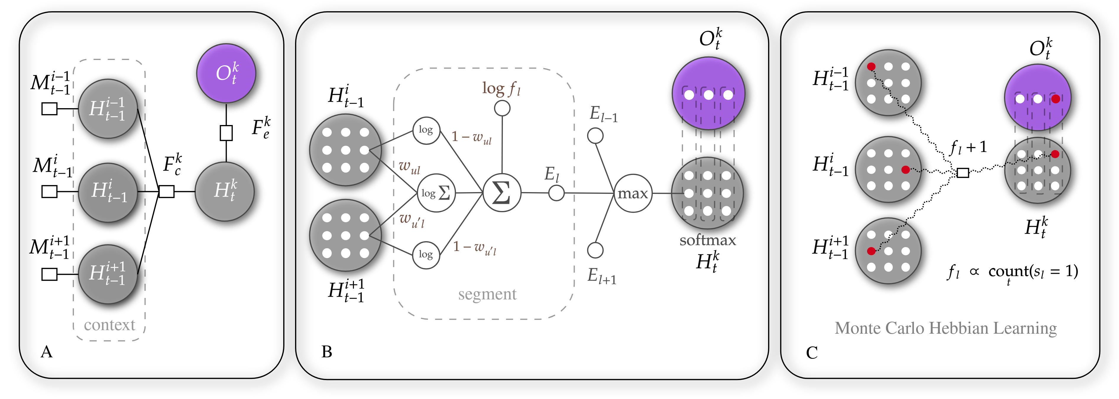
Figure 1: A. A factor graph for a single hidden variable and its context. Each hidden variable is considered to be independent of the others. $H^{k}_{t}$ and $O^{k}_{t}$ are hidden and observable random variables for a time step $t$. $F^{k}_{c}$ and $F^{k}_{e}$ are context and emission factors for the corresponding variables. Unary factors $M^{i}_{t-1}$ called messages represent information about previous time steps. B. Segment computations: estimate of segment activation probability and log-factor value $f_{l}$ determine effective cell excitation by segment $l$. C. Factor value learning involves sampling variable states from their posterior distributions in order to reinforce factor values for corresponding active segments.

We base our TM algorithm on the sum-product belief propagation algorithm in a factor graph shown in Figure 1A. Analogously to Factorial-HMM [14] we divide the hidden space $H$ into subspaces $H^{k}$ in our model of the environment. There are three sets of random variables (RV) in the model: $H^{i}_{t-1}$—hidden random variables representing hidden states from the previous time step (context), $H^{k}_{t}$—hidden random variables for the current time step, and $O^{k}_{t}$—observable random variables. All variables have a categorical distribution. RV state values are denoted as corresponding lowercase letters, i.e., $h^{i}_{t-1}$, $h^{k}_{t}$, $o^{k}_{t}$. For each $H^{k}_{t}$, we use a separate graphical model, considering them as independent to make our TM algorithm computationally efficient. However, hidden variables of the same time step are statistically interdependent in practice. We introduce their interdependence through a segment computation trick that goes beyond the standard sum-product algorithm. The model also has three types of factors: $M^{i}_{t-1}$—messages from previous time steps, $F^{k}_{c}$—context factor (generalized transition matrix), $F^{k}_{e}$—emission factor. We also assume that messages $M^{i}_{t-1}$ consider posterior information from the time step $t-1$. Therefore, we don’t depict observable variables for previous time steps.

The main routine of the algorithm is to estimate distributions of currently hidden state variables given by the equation 8, the computational flow of which is schematically depicted in Figure 1-B:

$$p(h_{t}^{k})\propto\sum_{\{h^{i}_{t-1}:i\in\omega_{k}\}}\prod_{i\in\omega_{k}}M_{t-1}^{i}(h_{t-1}^{i})F_{c}^{k}(h_{t}^{k},\{h^{i}_{t-1}:i\in\omega_{k}\}),$$ (8)

where $\omega_{k}={i_{1},\dots,i_{n}}$—set of previous time step RV indexes included in $F_{c}^{k}$ factor, $(n+1)$—factor size.

For computational purposes, we translate the problem to the neural network architecture with Hebbian-like learning. As can be seen from Figure 1-B, every RV can be viewed as a set of spiking neurons representing the RV’s states, that is, $p(h^{k}_{t})=p(c^{j}_{t}=1)$, where $j$—index of a neuron corresponding to the state $h^{k}_{t}$. Cell activity is binary $c^{j}_{t}\in\{0,1\}$ (spike/no-spike), and the probability might be interpreted as a spiking rate. Factors $F^{k}_{c}$ and $M^{i}_{t-1}$ can be represented as vectors, where elements are factor values for all possible combinations of RV states included in the factor. Let’s denote elements of the vectors as $f_{l}$ and $m_{u}$ correspondingly, where $l$ corresponds to a particular combination of $k,h^{k}_{t},h^{i_{1}}_{t-1},\dots,h^{i_{n_{l}}}_{t-1}$ state values and $u$ indexes all neurons representing states of previous time step RVs.

Drawing inspiration from biological neural networks, we introduce the notion of a segment that links together factor value $f_{l}$, the computational graph shown in Figure 1B, and the excitation $E_{l}$ induced by the segment $l$ to the cell it is attached to. A segment is a computational unit that detects a particular context state represented by its presynaptic cells. Analogously, dendritic segments of biological neurons known to be coincidence detectors of its synaptic input [40]. The segment is active, i.e., $s_{l}=1$ if all its presynaptic cells are active; otherwise, $s_{l}=0$. Computationally, a segment transmits its factor value $f_{l}$ to a cell it is attached to if the context matches the corresponding state combination.

We can now rewrite equation 8 as the following:

$$p(h_{t}^{k})\propto\sum_{l\in\mathrm{seg}(j)}L_{l}f^{k}_{l},$$ (9)

where $L_{l}=\prod_{u\in\mathrm{rec}(l)}m_{u}$ is segment’s likelihood as long as messages are normalized, $\mathrm{seg}(j)$—indexes of segments that are attached to cell $j$, $\mathrm{rec}(l)$—indexes of cells that constitute receptive field of segment with index $l$ (presynaptic cells).

Initially, all factor entries are zero, meaning cells have no segments. As learning proceeds, new segments are grown. As seen from equation 9, it can benefit from having sparse factor value vectors in this computational model, as its complexity grows linearly concerning the amount of non-zero components. And that’s usually the case in our model due to one-step Monte-Carlo learning and specific form of emission factors $F^{k}_{e}$:

$$F^{k}_{e}(h^{k}_{t},o^{k}_{t})=I[h^{k}_{t}\in\mathrm{col}(o^{k}_{t})],$$ (10)

where $I$—indicator function, $\mathrm{col}(o^{k}_{t})$ is a set of hidden states connected to the observational state $o^{k}_{t}$ that forms a column. The form of emission factor is inspired by presumably columnar structure of the neocortex and was shown to induce sparse transition matrix in HMM [13].

In this segment model, resulting from the sum-product algorithm, likelihood is calculated because presynaptic cells are independent. However, it’s not usually the case for sparse factors. To take into account the interdependence, we use the following equation for segment log-likelihood:

$$\log L_{l}=\log\sum_{u\in\mathrm{rec}(l)}w_{ul}m_{u}+\sum_{u\in\mathrm{rec}(l)}(1-w_{ul})\log m_{u}-\log n_{l},$$ (11)

where $w_{pl}$—synapse efficiency or neuron specificity for segment, so that $w_{ul}=p(s_{l}=1|c^{u}_{t-1}=1)$, and $n_{l}$-number of cells in segment’s receptive field.

The idea that underlies the formula is to approximate between two extreme cases:

• $p(s_{l}=1|c^{u}_{t-1}=1)\to 1$ for all $u$, which means that all cells in the receptive field are dependent and are part of one cluster, i.e., they fire together. In that case, it should be $p(s_{l})=m_{u}$ for any $u$, but we also reduce prediction variance by averaging between different $u$.

• $p(s_{l}=1|c^{u}_{t-1}=1)\to 0$ for all $u$ means that presynaptic cells don’t form a cluster. In that case, segment activation probability is just a product of the activation probability of each cell.

The resulting equation for belief propagation in DHTM is the following:

$$p(h^{k}_{t})=p(c^{j}_{t}=1) =\underset{j\in\mathrm{cells}[H^{k}_{t}]}{\mathrm{softmax}}(\underset{l\in seg(j)}{\mathrm{max}}(E_{l})),$$ (12)

$$E_{l} =\log f_{l}+\log L_{l},$$ (13)

where $\mathrm{cells}[H^{k}_{t}]$—indexes of cells that represent states for $H^{k}_{t}$ variable. Here, we also approximate logarithmic sum with $\mathrm{max}$ operation inspired by the neurophysiological model of segment aggregation by cell [40].

The next step after computing $p(h^{k}_{t})$ distribution parameters is to incorporate information about current observations $p(h^{k}_{t}\ |\ o^{k}_{t})\propto p(h^{k}_{t})I[h^{k}_{t}\in\mathrm{col}(o^{k}_{t})]$. After that, the learning step is performed. The step for closing the loop of our TM algorithm is to assign the posterior for the current step $p(h^{k}_{t}\ |\ o^{k}_{t})$ to $M^{i}_{t-1}$.

DHTM learns $f_{l}$ and $w_{ul}$ weights by Monte-Carlo Hebbian-like updates. First, $h^{i}_{t-1}$ and $h^{k}_{t}$ are sampled from their posterior distributions: $p(h^{i}_{t-1}\ |\ o^{i}_{t-1})\propto M^{i}_{t-1}$ and $p(h^{k}_{t}\ |\ o^{k}_{t})$ correspondingly. Then $f_{l}$ is updated according to the segment’s $s_{l}$ and its cell’s $c^{j}_{t}$ activity so that $f_{l}$ is proportional to several coincidences $s_{l}=c^{j}_{t}=1$ during the recent past, i.e., cell and its segment are active at the same time step, like shown in Figure 1C. It’s similar to Baum-Welch’s update rule [2] for the transition matrix in HMM, which, in effect, counts transitions from one state to another, but, in our case, the previous state (context) is represented by a group of RVs. Weights $w_{ul}$ are also updated by the Hebbian rule to reflect the specificity of a presynaptic $u$ for activating a segment $l$. If the activities of the presynaptic cell and its segment coincide, we increase $w_{ul}$; otherwise, $w_{ul}$ is decreased.

3.2 Agent Architecture

We test DHTM as a part of an agent in the RL task. The agent architecture is the same for all TM algorithms we compare to but with different memory modules. The agent consists of a memory model, SR representations, and an observation reward function. The memory model aims to speed up SR learning by predicting cumulative future distributions of observation variables according to equation 4. As shown in equation 5, SR representations are learned to estimate state value. The observation reward function is also learned during interaction with the environment and, combined with SR representations, is used to estimate the action value function.

Algorithm 1 Agent training procedure

1:  for episode=1..n do

2:     RESET_MEMORY()

3:     action $\leftarrow$ null

4:     while (not terminal) (steps $<$ max_steps) do

5:        obs, reward $\leftarrow$ STEP()

6:        obs* $\leftarrow$ ENCODE(PREPROCESS(obs))

7:        OBSERVE(obs*, action)

8:        REINFORCE(reward, obs*)

9:        action $\leftarrow$ SAMPLE_ACTION()

10:        ACT(action)

11:     end while

12:  end for

The agent training procedure is outlined in Algorithm 1. For each episode, the memory state is reset to a fixed initial message with RESET_MEMORY() and action variable is initialized with null value. An observation image returned by an environment (obs) is first preprocessed to get spiking events, mimicking a simple event-based camera with a floating threshold determined from the average difference between the current and previous step image intensities. The resulting events are encoded to SDRs with a biologically inspired spatial pooling encoder described in Appendix A.1. In OBSERVE() routine, the memory and SR learning happens as described in Section 3.1. An agent learns associations between observation states and rewards in line 8 and transforms them into observation priors $p(o^{k}_{t})$:

$$r^{k}_{i} \leftarrow r^{k}_{i}+\alpha I[o^{k}_{t}=i](R_{t}-r^{k}_{i})$$ (14)

$$p(o^{k}_{t}) =\mathrm{\underset{i}{softmax}(\lambda r^{k}_{i})}$$ (15)

where $\alpha$ is a learning rate, $R_{t}$—a reward for the current time step, $\lambda$—a reward scaling value. The logarithm of the observation prior serves as the value function used to estimate true state value, as shown in equation 2.

An agent has a softmax policy over predicted values: $\pi(a_{t}\ |\ o_{t})=\mathrm{softmax}(V[p(h_{t+1}\ |\ o_{t},a_{t})])$. We use the model to predict the hidden state distribution for every action in the next timestep $t+1$ and then estimate its value according to equation 6.

An episode continues until the terminal state or maximum steps are reached. An agent shares its memory weights between episodes.

4 Experiments

We test our agent in a pinball-like environment where SRs are easy to interpret. This section shows how different memory models affect SR learning and an agent’s adaptability. In our work, we compare the proposed DHTM model with LSTM [21], RWKV [36], and the factorial version of CHMM [13], which is several CHMMs trained in parallel independently.

Pinball is a partially observable environment developed in the Godot Game Engine [3]. A ball that can move in the surface’s 2D space and a surface with borders make up the environment (see Figure 2-A). Force fields depicted as circles introduce stochasticity to the environment as they deflect the ball in random directions. An agent can apply arbitrary momentum to a ball. For each time step, the environment returns an image of the top view of the table as an observation and a reward. The agent gets the reward by entering force fields. Each force field can be configured to pass a specific reward value and to terminate an episode.

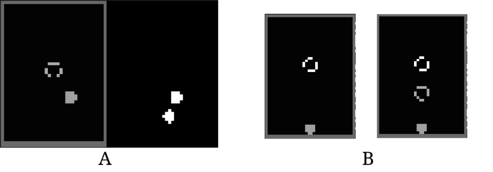
Figure 2: Examples of observations from the testing environment. A. Pinball environment with a viewing area of 50x36x1. On the right is the raw image, and on the left is the preprocessed binarized image of the ball’s movement. B. The experiments used two different setups. The left image shows a setup in which the target is not blocked. The image on the right depicts the setup, with the target obscured by a random field that deflects the ball perpendicular to its movement direction.

For our experiments, we use two configurations of the Pinball environment shown in Figure 2-B. We narrow the action space to three momentum vectors: vertical, 30 degrees left and 30 degrees right from the vertical axis. Each time step, the agent gets a small negative reward and a large positive reward if the ball enters the force field in the center. The episode finishes when the ball enters the force field or the maximum number of steps is reached. Each trial is run for 500 episodes, each a maximum of 15 steps long, and we average the results over three trials for each parameter set and memory model.

We first test the accuracy of five-step SR representations by measuring their pseudo-surprise, which is surprise computed for observed states on different time steps after SR was predicted with respect to normalized SR. The lower the surprise, the better SR’s quality. To form SR, we accumulate predictions of observations for five steps forward with a discount factor $\gamma=0.99$. As can be seen from Figure 3, SRs produced by our memory model (dhtm) give lower surprise than SRs of LSTM (lstm) and RWKV (rwkv), and is on par with SRs produced by Factorial version of CHMM (fchmm).

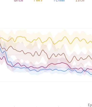
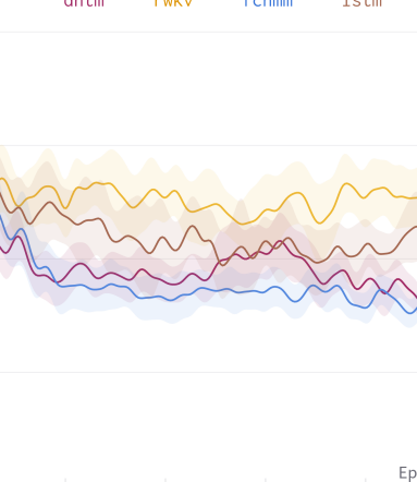
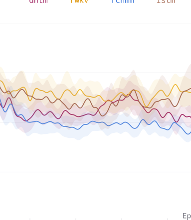
Figure 3: Surprise comparison for various memory models including DHTM, LSTM, RWKV, and Factorial CHMM. The SRs generated by normalized five-step prediction models are used to calculate surprise for three future time steps.

Then, we test how the number of prediction steps affects the agent’s adaptability in the Pinball environment. In the first 500 episodes, the agent is trained to reach the target in the center, as shown in Figure 2-B, then the target is blocked by a random force that applies force in perpendicular direction to the ball’s movement. That is, the previous optimal strategy becomes useless. The results show that an agent that uses five prediction steps during n-step TD learning of SR faster adapts to the changes in the environment inc comparison to 1-step TD learning for SR, as seen from Figure 4.

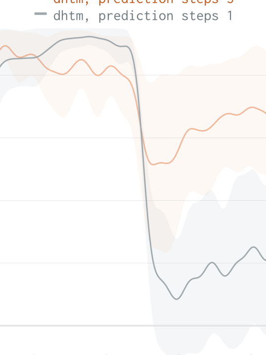
Figure 4: Comparison of agent’s adaptability during changes in the environment with different prediction steps during n-step TD learning of SR. At the 500th episode, the environment changes its configuration, shown in Figure 2.

5 Conclusion

In this paper we introduce a novel probabilistic Factorial-HMM-like algorithm DHTM for learning an observation sequence model in stochastic environments that uses local Hebbian-like learning rules and a transition matrix sparsification, which biologically plausible multicomponent neural models inspire. We show that our memory model can quickly learn the observation sequences representation and the transition dynamics. The DHTM produces more accurate n-step Successor Representations than LSTM and RWKV, which speeds up n-step TD learning of the SR in Reinforced Learning tasks with the changing environment.

Author Contributions

ED developed the theoretical foundations of the memory model and its software implementation, conducted experiments, and prepared the text of the article. PK developed the encoder and decoder, prepared and configured the LSTM and RWKV baselines. AP advised and supervised the work of the team. PK and AP also helped with writing the article.

Appendix A Appendix

A.1 Encoding and Decoding Observations

Because our model is designed to work with sparse distributed representations and the testing environments do not provide observations as SDRs by default, an encoding procedure is required. For this task, we use a modified version of the Spatial Pooler (SP) [5, 30], a distributed noise-tolerant online clustering neural network algorithm that converts input binary patterns into SDRs with fixed sparsity while retaining pairwise similarity [25]. The SP algorithm learns a spatial specialization of neurons’ receptive fields using the local Hebbian rule and k-WTA ($k$ winners take all) inhibition [33]. Here we outline the main differences from the “vanilla” version of the SP algorithm described in Cui et al. [5].

During an agent’s decision-making process pipeline, the SP encoder accepts a current observation $o$ and transforms it to a latent state SDR $z$. In terms of processing, our SP encoder functions as a standard artificial neural network with a k-WTA binary activation function.:

$$\text{overlaps}_{i} =\beta_{i}W_{i}o$$ (16)

$$z_{i} =I\left[i\in\text{kWTA}(\text{overlaps})\right],$$ (17)

where $o$—a binary observation vector, $W_{i}$—a row-vector representing $i$-th neuron’s connection weights (where non-existing connections have zero weights), $\text{overlaps}_{i}$—a value representing the strength of the input pattern recognition with the neuron $i$ , $\beta_{i}$—an $i$-th neuron boosting value, $z_{i}$—an $i$-th bit of an output SDR, $I[\dots]$—an indicator function, kWTA—a $k$-winners-take-all activation function returning $k$ indices of the neurons with the highest overlap.

One difference between the “vanilla” SP algorithm and ours is that we do not distinguish between potential and active neural connections. Because all [existing] connections are active, they all participate in calculating overlaps. In the overlaps calculation, non-binary, that is, real-valued weights are used, similar to artificial neural networks, as shown in equation 16. Furthermore, each neuron has a fixed capacity to produce neurotransmitters, which it distributes between its synaptic connections. This means that we keep all neuron weights normalized and summed to one. While it achieves the same Hebbian learning with homeostatic plasticity as the original SP, the exact formula is slightly different:

$$\tilde{W}_{i} =W_{i}+\alpha z_{i}\frac{\text{RF}_{i}\odot o}{\sum_{j}{\text{RF}_{i}\odot o}}$$

$$W_{i} \leftarrow\frac{\tilde{W}_{i}}{\sum_{j}{\tilde{W}_{i}}},$$ (18)

where $\tilde{W}_{i}$—a row of new $i$-th neuron weights before normalization, $\alpha$—learning rate, $z_{i}$—a binary value representing the current activity state of the $i$-th neuron, $RF_{i}$—an $i$-th row of the binary connectivity matrix representing an $i$-th neuron receptive field, $\odot$—elementwise product, $o$—a binary observation vector.

The original SP algorithm has several drawbacks, including encoding instability caused by an innate homeostatic plasticity mechanism known as boosting, which helps neurons specialize and increases overall adaptability but makes memorization tasks more difficult, and slow processing on large inputs such as images, where an encoding overhead becomes noticeable when compared to overall model timings around 1k input size.

The introduction of the newborn stage, which follows the ideas proposed in Dobric et al. [7], solves an encoding instability problem. The newborn stage of a spatial pooler occurs during the early stages of its learning process, when its neurons are expected to specialize. The boosting, which is intended to aid in the specialization process, is activated only during the newborn stage and its scale gradually decreases from the configured value to zero. Boosting remains turned off during an encoder’s “adulthood”, reducing the possibility of spontaneous re-specialization.

To reduce processing overhead, we use a much more sparsified connection matrix than in the original SP version. We randomly initialize connections with 40-60% sparsity, which is typical for the “vanilla” SP. Then, during the newborn stage, we gradually prune the vast majority of the weakest connections, resulting in neurons that are highly specialized due to their small receptive fields. We typically configure the final receptive field size in relation to the average input pattern size (usually 25-200% of it, resulting in 0.1-10% connections sparsity). For example, if binary input patterns have on average 100 active bits out of 1000, we can set the target size of receptive fields to 25, which is 25% of the active input size and corresponds to 2.5% connection matrix sparsity. As a result, the spatial pooler’s instability (and thus adaptiveness!) becomes even more limited in the adult stage.

Because of its soft discretization (from the distributed representation) and clusterization properties, we expect SP to assist the model with input sequence memorization and an environment transition dynamics generalization tasks in addition to the encoding itself. However, because the SP encoder learns online, particularly during the newborn stage, its output representation can be highly unstable during the early stages, potentially resulting in a performance drop.

To visualize and debug an encoded observation, we also learn a decoder, which is a linear neural layer learned locally with gradient descend on the MSE error between the predicted reconstruction and the actual observation.

References

- Barreto et al. [2017] André Barreto, Will Dabney, Rémi Munos, Jonathan J Hunt, Tom Schaul, Hado P van Hasselt, and David Silver. Successor features for transfer in reinforcement learning. Advances in neural information processing systems, 30, 2017.
- Baum et al. [1970] Leonard E Baum, Ted Petrie, George Soules, and Norman Weiss. A maximization technique occurring in the statistical analysis of probabilistic functions of markov chains. The annals of mathematical statistics, 41(1):164–171, 1970.
- Beeching et al. [2021] Edward Beeching, Jilles Debangoye, Olivier Simonin, and Christian Wolf. Godot reinforcement learning agents. arXiv preprint arXiv:2112.03636, 2021.
- Churchland & Sejnowski [1992] Patricia Smith Churchland and Terrence Joseph Sejnowski. The computational brain. MIT press, 1992.
- Cui et al. [2017] Yuwei Cui, Subutai Ahmad, and Jeff Hawkins. The htm spatial pooler—a neocortical algorithm for online sparse distributed coding. Frontiers in Computational Neuroscience, 11:111, 2017. ISSN 1662-5188. doi: 10.3389/fncom.2017.00111. URL https://www.frontiersin.org/article/10.3389/fncom.2017.00111.
- Dayan [1993] Peter Dayan. Improving generalization for temporal difference learning: The successor representation. Neural computation, 5(4):613–624, 1993.
- Dobric et al. [2022] Damir Dobric, Andreas Pech, Bogdan Ghita, and Thomas Wennekers. On the importance of the newborn stage when learning patterns with the spatial pooler. SN Computer Science, 3(2):179, 2022.
- Dwivedi et al. [2023] Yogesh K Dwivedi, Nir Kshetri, Laurie Hughes, Emma Louise Slade, Anand Jeyaraj, Arpan Kumar Kar, Abdullah M Baabdullah, Alex Koohang, Vishnupriya Raghavan, Manju Ahuja, et al. “so what if chatgpt wrote it?” multidisciplinary perspectives on opportunities, challenges and implications of generative conversational ai for research, practice and policy. International Journal of Information Management, 71:102642, 2023.
- Eraslan et al. [2019] Gökcen Eraslan, Žiga Avsec, Julien Gagneur, and Fabian J Theis. Deep learning: new computational modelling techniques for genomics. Nature Reviews Genetics, 20(7):389–403, 2019.
- Friston et al. [2016] Karl Friston, Thomas FitzGerald, Francesco Rigoli, Philipp Schwartenbeck, Giovanni Pezzulo, et al. Active inference and learning. Neuroscience & Biobehavioral Reviews, 68:862–879, 2016.
- Friston et al. [2018] Karl J Friston, Richard Rosch, Thomas Parr, Cathy Price, and Howard Bowman. Deep temporal models and active inference. Neuroscience & Biobehavioral Reviews, 90:486–501, 2018.
- George & Hawkins [2009] Dileep George and Jeff Hawkins. Towards a mathematical theory of cortical micro-circuits. PLoS computational biology, 5(10):e1000532, 2009.
- George et al. [2021] Dileep George, Rajeev V. Rikhye, Nishad Gothoskar, J. Swaroop Guntupalli, Antoine Dedieu, and Miguel Lázaro-Gredilla. Clone-structured graph representations enable flexible learning and vicarious evaluation of cognitive maps. Nature Communications, 12(11):2392, Apr 2021. ISSN 2041-1723. doi: 10.1038/s41467-021-22559-5.
- Ghahramani & Jordan [1997] Z. Ghahramani and M.I. Jordan. Factorial Hidden Markov Models. Machine Learning, 29(2-3):245–273, 1997. ISSN 0885-6125. doi: 10.1023/a:1007425814087.
- Ghahramani & Jordan [1995] Zoubin Ghahramani and Michael Jordan. Factorial hidden markov models. Advances in neural information processing systems, 8, 1995.
- Ha & Schmidhuber [2018] David Ha and Jürgen Schmidhuber. World models. arXiv preprint arXiv:1803.10122, 2018.
- Hafner et al. [2023] Danijar Hafner, Jurgis Pasukonis, Jimmy Ba, and Timothy Lillicrap. Mastering diverse domains through world models. arXiv preprint arXiv:2301.04104, 2023.
- Harshvardhan et al. [2020] GM Harshvardhan, Mahendra Kumar Gourisaria, Manjusha Pandey, and Siddharth Swarup Rautaray. A comprehensive survey and analysis of generative models in machine learning. Computer Science Review, 38:100285, 2020.
- Hawkins & Ahmad [2016] Jeff Hawkins and Subutai Ahmad. Why neurons have thousands of synapses, a theory of sequence memory in neocortex. Frontiers in Neural Circuits, 10, March 2016. ISSN 1662-5110. doi: 10.3389/fncir.2016.00023. URL http://journal.frontiersin.org/Article/10.3389/fncir.2016.00023/abstract.
- Hebb [2005] Donald Olding Hebb. The organization of behavior: A neuropsychological theory. Psychology press, 2005.
- Hochreiter & Schmidhuber [1997] Sepp Hochreiter and Jürgen Schmidhuber. Long short-term memory. Neural computation, 9:1735–80, 12 1997. doi: 10.1162/neco.1997.9.8.1735.
- Jahromi et al. [2022] Mehdi Jafarnia Jahromi, Rahul Jain, and Ashutosh Nayyar. Online learning for unknown partially observable mdps. In International Conference on Artificial Intelligence and Statistics, pp. 1712–1732. PMLR, 2022.
- Ji et al. [2020] Shulei Ji, Jing Luo, and Xinyu Yang. A comprehensive survey on deep music generation: Multi-level representations, algorithms, evaluations, and future directions. arXiv preprint arXiv:2011.06801, 2020.
- Kschischang et al. [2001] F.R. Kschischang, B.J. Frey, and H.-A. Loeliger. Factor graphs and the sum-product algorithm. IEEE Transactions on Information Theory, 47(2):498–519, 2001. doi: 10.1109/18.910572.
- Kuderov et al. [2023] Petr Kuderov, Evgenii Dzhivelikian, and Aleksandr I Panov. Stabilize sequential data representation via attraction module. In International Conference on Brain Informatics, pp. 83–95. Springer, 2023.
- Lillicrap et al. [2020] Timothy P. Lillicrap, Adam Santoro, Luke Marris, Colin J. Akerman, and Geoffrey Hinton. Backpropagation and the brain. Nature Reviews Neuroscience, 21(6):335–346, Jun 2020. ISSN 1471-003X, 1471-0048. doi: 10.1038/s41583-020-0277-3.
- Lipton et al. [2015] Zachary C Lipton, John Berkowitz, and Charles Elkan. A critical review of recurrent neural networks for sequence learning. arXiv preprint arXiv:1506.00019, 2015.
- Mathys et al. [2011] Christoph Mathys, Jean Daunizeau, Karl J Friston, and Klaas E Stephan. A bayesian foundation for individual learning under uncertainty. Frontiers in human neuroscience, 5:39, 2011.
- Min et al. [2021] Bonan Min, Hayley Ross, Elior Sulem, Amir Pouran Ben Veyseh, Thien Huu Nguyen, Oscar Sainz, Eneko Agirre, Ilana Heintz, and Dan Roth. Recent advances in natural language processing via large pre-trained language models: A survey. ACM Computing Surveys, 2021.
- Mnatzaganian et al. [2017] James Mnatzaganian, Ernest Fokoué, and Dhireesha Kudithipudi. A mathematical formalization of hierarchical temporal memory’s spatial pooler. Frontiers in Robotics and AI, 3, 2017. ISSN 2296-9144. URL https://www.frontiersin.org/articles/10.3389/frobt.2016.00081.
- Moerland et al. [2023] Thomas M Moerland, Joost Broekens, Aske Plaat, Catholijn M Jonker, et al. Model-based reinforcement learning: A survey. Foundations and Trends® in Machine Learning, 16(1):1–118, 2023.
- Orvieto et al. [2023] Antonio Orvieto, Samuel L Smith, Albert Gu, Anushan Fernando, Caglar Gulcehre, Razvan Pascanu, and Soham De. Resurrecting recurrent neural networks for long sequences. arXiv preprint arXiv:2303.06349, 2023.
- Oster et al. [2009] Matthias Oster, Rodney Douglas, and Shih-Chii Liu. Computation with spikes in a winner-take-all network. Neural Computation, 21(9):2437–2465, 09 2009. doi: 10.1162/neco.2009.07-08-829.
- O’Reilly et al. [2021] Randall C. O’Reilly, Jacob L. Russin, Maryam Zolfaghar, and John Rohrlich. Deep predictive learning in neocortex and pulvinar. Journal of Cognitive Neuroscience, 33(6):1158–1196, May 2021. ISSN 0898-929X. doi: 10.1162/jocn_a_01708.
- Parr & Friston [2017] Thomas Parr and Karl J Friston. Working memory, attention, and salience in active inference. Scientific reports, 7(1):14678, 2017.
- Peng et al. [2023] Bo Peng, Eric Alcaide, Quentin Anthony, Alon Albalak, Samuel Arcadinho, Huanqi Cao, Xin Cheng, Michael Chung, Matteo Grella, Kranthi Kiran GV, et al. Rwkv: Reinventing rnns for the transformer era. arXiv preprint arXiv:2305.13048, 2023.
- Perin et al. [2011] Rodrigo Perin, Thomas K Berger, and Henry Markram. A synaptic organizing principle for cortical neuronal groups. Proceedings of the National Academy of Sciences, 108(13):5419–5424, 2011.
- Poupart [2005] Pascal Poupart. Exploiting structure to efficiently solve large scale partially observable Markov decision processes. Citeseer, 2005.
- Salaün et al. [2019] Achille Salaün, Yohan Petetin, and François Desbouvries. Comparing the modeling powers of rnn and hmm. In 2019 18th ieee international conference on machine learning and applications (icmla), pp. 1496–1499. IEEE, 2019.
- Stuart & Spruston [2015] Greg J. Stuart and Nelson Spruston. Dendritic integration: 60 years of progress. Nature Neuroscience, 18(12):1713–1721, Dec 2015. ISSN 1546-1726. doi: 10.1038/nn.4157. URL https://doi.org/10.1038/nn.4157.
- Zhao et al. [2020] Jingyu Zhao, Feiqing Huang, Jia Lv, Yanjie Duan, Zhen Qin, Guodong Li, and Guangjian Tian. Do rnn and lstm have long memory? In International Conference on Machine Learning, pp. 11365–11375. PMLR, 2020.