A magnetic clock for a harmonic oscillator

Abstract

We present an implementation of a recently proposed procedure for defining time, based on the description of the evolving system and its clock as non-interacting, entangled systems, according to the Page and Wootters approach. We study how the quantum dynamics transforms into a classical-like behaviour when conditions related with macroscopicity are met by the clock alone, or by both the clock and the evolving system. In the description of this emerging behaviour finds its place the classical notion of time, as well as that of phase-space and trajectories on it. This allows us to analyze and discuss the relations that must hold between quantities that characterize system and clock separately, in order for the resulting overall picture be that of a physical dynamics as we mean it.

I Introduction

In the conventional formulation of Quantum Mechanics (QM) Dirac_PQM_1958 ; Peres2002 time is an external parameter, not related with any observable of the system; this somehow anomalous status is often considered a weakness of the theory, referred to as ”the problem of time” MugaME2002book , mining the capacity of QM to describe the facets of the physical world. One of the most promising proposal for ”solving” such problem by treating time as a quantum observable emerged some decades agoPageW83 in the realm of quantum information, and goes under the name of ”Page and Wootters (PaW) mechanism”. The mechanism is based on the idea that the actual time $t$ for an evolving system is set by the fact that another system (referred to as the ”clock”) be in a state labelled by the value $t$. The idea takes shape in the quantum formalism, with system and clock together assumed in an entangled state. The PaW proposal has been the subject of careful analysis in the following decades and a convincing answer has been finally found for many criticisms originally raised against it GiovannettiLM15 ; MarlettoV17 ; BryanM18 ; SmithA19 ; AltaieHB22 . Moreover, in recent years it has been shown how the PaW mechanism can be employed to operationally define local time reference frames associated with several quantum clocks, allowing for time dilation and gravitational interactionCastro-RuizGBB20 , and a generalization of the PaW formalism has been proposed to investigate the causal structure of processes in general relativityBaumannKGB22 . The relationship of the PaW formalism with other approaches to quantum gravity and, more generally, to quantum mechanicsRovelli96 and to the definition of (time-) reference frames, quantum observables and their classical limit has also been addressedChataignier21 .

Within the framework of the PaW mechanism, we have recently FCBCVnat21 derived both the quantum Schrödinger equation and the classical Hamilton equations of motion exclusively enforcing the conditions set by the PaW mechanism, in a way that consistently identifies the physical quantity that plays the role of time in both equations.

Aim of this work is to present an explicit realization of the procedure introduced in Ref. FCBCVnat21 . Elements of our picture are two non-interacting and yet entangled systems: one is the clock $C$, described as a magnetic system, and the other is the evolving system $\Gamma$, chosen as a harmonic oscillator. We will show that $C$ can describe the standard dynamics of $\Gamma$, regardless of whether the latter is quantum or classical. In addition, the explicit realization offers the possibility to carefully analyze all the details of the actual implementation of the PaW mechanism, allowing us to reveal the connection between the physical properties of $C$ and its capability of properly describe the dynamics of $\Gamma$.

The structure of the paper is as follows: in Sec. II we introduce the pair $\Gamma$ and $C$, with details about their respective Hamiltonians. In Sec. III we discuss the fully quantum model, defining all the relevant quantities characterizing the entangled state of the two subsystems, while in Sec. IV, after having introduced the proper formalism allowing us to let just one of the two subsystems (the clock $C$) to become macroscopic and amenable of a classical description, we are able to explicitly relate the parameters describing $C$ with the energy of the system $\Gamma$ and its dynamics, showing how the energy scale of $C$ reflects on its ability to describe the dynamics of the evolving system $\Gamma$ in its entire Hilbert space. In Sec. V the classical limit of both $C$ and $\Gamma$ is taken, in such a way to not only recover the classical Hamilton’s Equations of Motion (EoM), but getting also directly the classical orbits in phase space. Finally, in the last Section, we discuss the main results and draw our conclusions.

II The overall quantum system

In Quantum Mechanics (QM) any physical system is described by a theory defined by some representation of a Lie-algebra $\mathfrak{g}$, i.e. by a Hilbert space ${\cal H}$ and the commutation relations $[\,\cdot,\cdot\,]$ between the operators acting on ${\cal H}$ that describe the observables of the system. The specific algebra is identified by requiring that the Hamiltonian $\hat{H}$ ruling the dynamical evolution of the system belongs to $\mathfrak{g}$.

In this work we consider two systems, $\Gamma$ and $C$.
$\Gamma$ belongs to the family of bosonic systems, described by the Lie algebra $\mathfrak{h}_{4}$, whose representation on some infinite-dimensional Hilbert space is spanned by the operators $\{\hat{a},\hat{a}^{\dagger},\hat{n}=\hat{a}^{\dagger}\hat{a},\hat{\mathbb{I}}\}$ such that $[\hat{a},\hat{a}^{\dagger}]=\hat{\mathbb{I}}$. In particular, $\Gamma$ is a harmonic oscillator with mass $M$ and frequency $\omega$. For reasons that will be clearer later, we introduce the normalized bosonic operators $\hat{\mathsf{a}}^{(\dagger)}:=\hat{a}^{(\dagger)}/\sqrt{M}$, such that

$$\left[\hat{\mathsf{a}},\hat{\mathsf{a}}^{\dagger}\right]=\frac{\hat{\mathbb{I}}}{M}~{},$$ (1)

in terms of which, setting $\hbar=1$ from now on, the Hamiltonian of $\Gamma$ reads

$$\hat{H}_{{}_{{\Gamma}\,}}:=\frac{\hat{p}^{2}}{2M}+\frac{1}{2}M\omega^{2}\hat{q}^{2}=\omega M\left(\hat{\mathsf{n}}+\frac{\hat{\mathbb{I}}}{2M}\right)$$ (2)

with $\hat{\mathsf{n}}:=\hat{\mathsf{a}}^{\dagger}\hat{\mathsf{a}}$, $\hat{q}:=\sqrt{\frac{1}{2\omega}}(\hat{\mathsf{a}}^{\dagger}+\hat{\mathsf{a}})$, and $\hat{p}:=M\sqrt{\frac{\omega}{2}}(\hat{\mathsf{a}}^{\dagger}-\hat{\mathsf{a}})$.

In this work $\Gamma$ is the evolving system, whose time is possibly marked by $C$, as defined below.

$C$ belongs to the family of spin systems, described by the Lie algebra $\mathfrak{su}(2)$, whose representation on some $(2J+1)$-dimensional Hilbert space is spanned by the operators $\{\hat{J}_{0},\hat{J}_{1},\hat{J}_{2}\}$ such that $[\hat{J}_{i},\hat{J}_{j}]=i\epsilon_{ijk}\hat{J}_{k}$ with $i(j,k)=0,1,2$, and the Casimir $\hat{J_{0}}^{2}$+$\hat{J_{1}}^{2}$+$\hat{J_{2}}^{2}$= $J(J+1)\hat{\mathbb{I}}$ that provides the spin $J$ of the system. In particular, $C$ is a spin-$J$ system in the presence of a magnetic field pointing in a direction labelled by the above index $0$. We use the normalized spin operators $\hat{\mathsf{j}}_{i}:=\hat{J}_{i}/J$, such that

$$[\hat{\mathsf{j}}_{i},\hat{\mathsf{j}}_{j}]=\frac{i}{J}\,\hat{\mathsf{j}}_{k}\,\epsilon_{ijk}\,,$$ (3)

in terms of which the Hamiltonian of $C$ reads

$$\hat{H}_{{}_{{C}\,}}=\epsilon J\,\hat{\mathsf{j}}_{0}+F\,\hat{\mathbb{I}}~{},$$ (4)

with $\epsilon J$ and $F$ positive energies. In this work $C$ is the clock that marks the time for the evolution of $\Gamma$.

Referring to the PaW mechanism, we assume that $\Gamma$ and $C$ do not interact, and consequently write the Hamiltonian of the composite system $\Psi=C+\Gamma$ as

$$\hat{H}=\hat{H}_{{}_{{C}\,}}\otimes\hat{\mathbb{I}}_{{}_{{\Gamma}\,}}-\hat{\mathbb{I}}_{{}_{{C}\,}}\otimes\hat{H}_{{}_{{\Gamma}\,}}~{};$$ (5)

moreover, consistently with the fact that there is no other system, i.e. $\Psi$ is isolated, we require it to be in a pure state $\ket{\Psi}\!\rangle$ such that

$$\hat{H}\ket{\Psi}\!\rangle=0~{},$$ (6)

$$\ket{\Psi}\!\rangle\;\mbox{is entangled}~{},$$ (7)

where the double bracket in $\ket{~{}\cdot~{}}\!\rangle$ is used to indicate a vector in a Hilbert space that is the tensor product of two distinct Hilbert spaces or, which is the same, remind one that $\Psi$ is a composite system made of the two distinct subsystems $\Gamma$ and $C$. The conditions (6)-(7) set the framework for the PaW mechanism and are quite often questioned, particularly as far as the possibility that an eigenstate of a non-interacting Hamiltonian be entangled. Although this should not surprise (just think to the maximally entangled Bell singlet of two qubits A and B, which is one of the eigenstates of a non-interacting Hamiltonian proportional to $\hat{J}^{A}_{0}+\hat{J}^{B}_{0}$), it is true that the PaW constraints are fulfilled only for some specific states of $\Gamma$ and $C$, whose identification is not trivial, as we show below.

III A quantum magnetic clock for a quantum oscillator

In this section we use a quantum description for both $C$ and $\Gamma$. Their Hilbert spaces $\mathcal{H}_{{}_{{C}\,}}$ and $\mathcal{H}_{{}_{{\Gamma}\,}}$, spanned by $\{\ket{J,m},~{}m=-J,-J+1,...,J\}$ and $\{\ket{n},~{}n\in\mathbb{N}\}$ respectively, are irreducible representations of $\mathfrak{su}(2)$ and $\mathfrak{h}_{4}$ defined via

$$\begin{cases}\hat{\mathsf{j}}_{0}\ket{J,m}_{{}_{{C}\,}}=\frac{m}{J}\ket{J,m}_{{}_{{C}\,}}\;\;\;2J\in\mathbb{N},\;\;m=\{-J,...,J\}~{},\\ \hat{\mathsf{n}}\ket{n}_{{}_{{\Gamma}\,}}=\frac{n}{M}\ket{n}_{{}_{{\Gamma}\,}}\;\;\;n\in\mathbb{N}~{};\end{cases}$$ (8)

without loss of generality we take $F=\epsilon J$ so that $\hat{H}_{{}_{{C}\,}}\ket{J,-J}_{{}_{{C}\,}}=0$.

Any state of $\Psi$ can be written as

$$\ket{\Psi}\!\rangle=\sum_{n=0}^{\infty}\sum_{m=-J}^{J}c_{nm}\ket{J,m}_{{}_{{C}\,}}\ket{n}_{{}_{{\Gamma}\,}}\;\;\mbox{with}\;\;\sum_{n,m}|c_{nm}|^{2}=1~{},$$ (9)

referred to which the constraint (6) takes the form

$$\sum_{n,m}c_{nm}\left[\epsilon(m+J)-M\omega\left(n+\frac{1}{2}\right)\right]\ket{J,m}_{{}_{{C}\,}}\ket{n}_{{}_{{\Gamma}\,}}=0~{},$$ (10)

implying

$$c_{nm}=c_{m}\;\delta\left[\epsilon(m+J)-\omega\left(n+\frac{1}{2}\right)\right]~{}.$$ (11)

This means that in order for the coefficients $c_{nm}$ to be different from zero the quantum numbers $n$ and $m$ must satisfy

$$n+\frac{1}{2}=\kappa r\left(m+J\right)~{},$$ (12)

with

$$\kappa:=\frac{\epsilon J}{\omega M}~{}{\rm and}~{}r:=\frac{M}{J}~{}.$$ (13)

So, for the constraint (6) to hold, once $\kappa$ and $r$ are fixed, only some states $\ket{J,m}_{{}_{{C}\,}}\ket{n}_{{}_{{\Gamma}\,}}$ can enter the decomposition (9). If we consider for instance $\kappa r=3/4$, it is $n+1/2=3(m+J)/4$, and hence, depending on the value of $J$, it is

$$J<1 \rightarrow \nexists\,(m,n)$$

$$J=1 \rightarrow (m=1,n=1)$$

$$J=3/2 \rightarrow (m=1/2,n=1)$$

$$J=2 \rightarrow (m=0,n=1)$$

$$J=5/2 \rightarrow (m=-1/2,n=1)$$

$$J=3 \rightarrow (m=-1,n=1)\,\vee\,(m=3,n=4)$$

$$...~{},$$ (14)

where $\rightarrow$ stands for ”quantum numbers of the allowed states”. Moreover, since $\ket{\Psi}\!\rangle$ must be entangled, as required by (7), there must be at least two pairs $(m,n)$ that satisfy Eq. (12); in the above considered case $\kappa r=3/4$, for instance, it must hence be $J\geq 3$. In the most general case it can be shown (see App. A) that there exist pairs $(m,n)$ such that conditions (6) and (7) hold for $\ket{\Psi}\!\rangle$ if

$$\kappa r = \frac{2i_{n}+1}{2i_{m}}~{}~{},~{}~{}i_{m},i_{n}\in{\mathbb{N}}~{},$$ (15)

$$m = i_{m}(2l+1)-J~{}~{},~{}~{}n=i_{n}(2l+1)+l~{},$$ (16)

$${\rm with}~{}l=0,1,2,...,\left\lfloor J/i_{m}-1/2\right\rfloor~{},$$ (17)

$${\rm and}~{}J\geq 3i_{m}/2~{},$$ (18)

where the last inequality ensures that there are at least two allowed $(m,n)$ pairs, i.e. that $\ket{\Psi}\!\rangle$ is entangled. In the previous example $\kappa r=3/4$, it is $i_{n}=1,i_{m}=2$, $J\geq 3$, and $\{(m,n)\}=\{(4l+2-J,3l+1),\,l=0,1,..,\lfloor J/2-1/2\rfloor\}$.

When Eq. (12) holds, the coefficients in (9) depend on one index only, say $m$, and one can write

$$\ket{\Psi}\!\rangle=\sum_{m\in\mathcal{A}}c_{m}\ket{J,m}_{{}_{{C}\,}}\ket{n_{m}}_{{}_{{\Gamma}\,}}~{},~{}n_{m}\coloneqq\kappa r(m+J)-\frac{1}{2}~{},$$ (19)

with $\mathcal{A}$ the set of integers $m$ consistent with Eqs. (15)-(18). Following Ref. FCBCVnat21 , we introduce Generalized Coherent States (GCS) for the clock, i.e. the $\mathfrak{su}(2)$-CS also known as Spin Coherent States (SCS), defined as

$$\ket{\Omega}_{{}_{{C}\,}}:=e^{\Omega\hat{J}_{+}-\Omega^{*}\hat{J}_{-}}\ket{J,-J}_{{}_{{C}\,}}~{},~{}~{}\ket{\Omega}\leftrightarrow\Omega(\theta,\varphi)\in S^{2}~{},$$ (20)

where $\hat{J}_{\pm}=\hat{J}_{1}\pm i\hat{J}_{2}$, and $\Omega(\theta,\varphi)=(\theta/2)e^{-i\varphi}$. These states are in one-to-one correspondence with the points of the sphere $S^{2}$, as easily seen by recognizing $(\theta,\varphi)\in[0,\pi]\times[0,2\pi)$ as the usual polar coordinates.

Partially projecting $\ket{\Psi}\!\rangle$ upon SCS of $C$, the following unnormalized elements of $\mathcal{H}_{{}_{{\Gamma}\,}}$ are obtained

$$\ket{\Phi_{\theta}(\varphi)}_{{}_{{\Gamma}\,}}\coloneqq\braket{\Omega}{\Psi}\!\rangle=\sum_{m\in\mathcal{A}}c_{m}\braket{\Omega}{J,m}\,\ket{n_{m}}_{{}_{{\Gamma}\,}}$$ (21)

$$=\sum_{m\in\mathcal{A}}c_{m}\binom{2J}{m+J}^{1/2}\left(\cos\frac{\theta}{2}\right)^{J-m}\left(\sin\frac{\theta}{2}\right)^{J+m}$$

$$\qquad\qquad\quad e^{-i\varphi(J+m)}\ket{n_{m}}_{{}_{{\Gamma}\,}}~{},$$

where the specific form of $\braket{\Omega}{J,m}$ can be found, for instance, in Ref. Perelomov86 . Notice that taking $\varphi$ in $[0,\infty)$, rather than in $[0,2\pi)$, implies no ambiguity and can be safely done.

The state $\ket{\Phi_{\theta}(\varphi)}_{{}_{{\Gamma}\,}}$ obeys FCBCVnat21

$$i\epsilon\frac{d}{d\varphi}\ket{\Phi_{\theta}(\varphi)}_{{}_{{\Gamma}\,}}=\hat{H}_{{}_{{\Gamma}\,}}\ket{\Phi_{\theta}(\varphi)}_{{}_{{\Gamma}\,}}~{},$$ (22)

a differential equation that has the form of the Schrödinger equation, with $\varphi/\epsilon$ as time, and yet does not describe the unitary dynamics of pure states, for two reasons: first, $\ket{\Phi_{\theta}(\varphi)}_{{}_{{\Gamma}\,}}$ has a dependence on a further external parameter $\theta$ that makes no sense if $\Gamma$ is isolated, as required for the Schrödinger equation to hold. Second, $\ket{\Phi_{\theta}(\varphi)}_{{}_{{\Gamma}\,}}$ is not a physical state of $\Gamma$ because it is unnormalized. In fact, this latter reason is most often considered amendable (as done for instance in Refs. PageW83 ; GiovannettiLM15 ), since the same differential equation

$$i\epsilon\frac{d}{d\varphi}\ket{\phi_{\theta}(\varphi)}_{{}_{{\Gamma}\,}}=\hat{H}_{\Gamma}\ket{\phi_{\theta}(\varphi)}_{{}_{{\Gamma}\,}}~{},$$ (23)

holds for the normalized state

$$\ket{\phi_{\theta}(\varphi)}_{{}_{{\Gamma}\,}}:=\frac{\ket{\Phi_{\theta}(\varphi)}_{{}_{{\Gamma}\,}}}{\chi^{2}(\theta)}~{},$$ (24)

given that

$$\chi^{2}(\theta):=\langle{\Phi_{\theta}(\varphi)|\Phi_{\theta}(\varphi)}\rangle_{{}_{{\Gamma}\,}}=\sum_{m\in\mathcal{A}}|c_{m}|^{2}\,\left|\braket{\Omega}{J,m}\right|^{2}$$ (25)

$$=\sum_{m\in\mathcal{A}}|c_{m}|^{2}\binom{2J}{m+J}\left(\cos\frac{\theta}{2}\right)^{2(J-m)}\left(\sin\frac{\theta}{2}\right)^{2(J+m)}~{},$$ (26)

is a positive function that does not depend on $\varphi$. Notice that Eq. (24) defines a physical state for $\Gamma$ for any $\theta$ such that $\chi(\theta)\neq 0$. In fact, the role played by $\chi^{2}(\theta)$ goes well beyond its being the norm of $\ket{\Phi_{\theta}(\varphi)}_{{}_{{\Gamma}\,}}$, as will be clear once the parametric representation with GCS is introduced. Whether one thinks the above ad hoc normalization to be a satisfactory solution or not, neither Eq. (22) nor its sibling for the normalized state $\ket{\phi_{\theta}(\varphi)}_{{}_{{\Gamma}\,}}$ should be considered equations of motion, at this stage, as best explained by the following example.

Let us take $\kappa r=3/4$ and $J=3$ in Eq. (12), i.e. (see (14)) $c_{-1}=c_{3}=1/\sqrt{2}$, and $c_{m}=0$ otherwise. In this case, the sum in Eq. (26) reduces to just two terms,

$$\chi^{2}(\theta)=\frac{15}{2}\left(\cos\frac{\theta}{2}\right)^{8}\left(\sin\frac{\theta}{2}\right)^{4}+\frac{1}{2}\left(\sin\frac{\theta}{2}\right)^{12}~{},$$ (27)

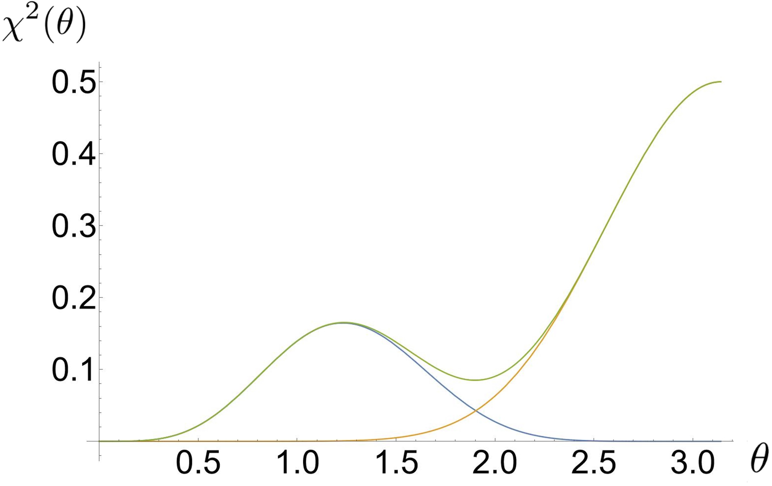
Figure 1: Graphical representations of $\frac{1}{2}\left|\braket{\Omega}{3,-1}\right|^{2}$ (blue line), $\frac{1}{2}\left|\braket{\Omega}{3,3}\right|^{2}$ (orange line), and $\chi^{2}(\theta)$ (green line), as defined in Eqs.(26)-(27).

that simultaneously vanish for $\theta=0$ only, as seen in Fig. 1. Therefore, any $\theta\in(0,\pi)$ defines a normalized state for $\Gamma$, that reads

$$\ket{\phi_{\theta}(\varphi)}_{{}_{{\Gamma}\,}} = \frac{\sqrt{15}\left(\cos\frac{\theta}{2}\right)^{4}}{\sqrt{15\left(\cos\frac{\theta}{2}\right)^{8}+\left(\sin\frac{\theta}{2}\right)^{8}}}e^{-2i\varphi}\ket{1}_{{}_{{\Gamma}\,}}$$ (28)

$$+ \frac{\left(\sin\frac{\theta}{2}\right)^{4}}{\sqrt{15\left(\cos\frac{\theta}{2}\right)^{8}+\left(\sin\frac{\theta}{2}\right)^{8}}}e^{-6i\varphi}\ket{4}_{{}_{{\Gamma}\,}}~{}.$$

This expression shows one of the most relevant features of this fully quantum setting, namely that once the parameters of the Hamiltonians (2) and (4), are fixed, the system $C$ can mark the time for the evolution of $\Gamma$ via the PaW mechanism only if its dynamics is limited to a subspace of $\mathcal{H}_{{}_{{\Gamma}\,}}$, defined by $M,\omega,\epsilon$, and the Casimir $J$. In the above example, where $\kappa r=3/4$ and $J=3$, for instance, the $\varphi$-derivation of the state (28) leads to a differential equation that cannot describe the appearance of elements of ${\cal H}_{{}_{{\Gamma}\,}}$ others than $\ket{1}_{{}_{{\Gamma}\,}}$ and $\ket{4}_{{}_{{\Gamma}\,}}$. In general, the finiteness of the Casimir $J$ in Eqs. (16) and (17) sets an upper limit for $n$, which prevents $\ket{\phi_{\theta}(\varphi)}_{{}_{{\Gamma}\,}}$ to explore its infinite-dimensional Hilbert space as time goes by. One could clearly observe that it is absolutely not surprising that difficulties arise when one tries to label states of an infinite-dimensional Hilbert space by states of a finite dimensional one. However, we see that even if we consider the equally possible symmetrical setting, where the harmonic oscillator plays the role of the clock and the spin system is the evolving system whose dynamics we are interested to describe, we can still be unable to properly explore the full Hilbert space of the evolving system, unless further adjustment is made, e.g. properly shifting the ground state of the clock or the evolving system.

This result may sound puzzling, as we are used to consider clocks as objects whose capability of marking the time does not depend on the specific evolution that unfolds in such time, no matter whether in quantum or classical physics. A useful analogy to solve this conundrum comes from considering any model where an external magnetic field is applied to a quantum magnetic system via a Zeeman interaction ${\mathbf{h}}\cdot{\hat{\mathbf{S}}}$. In this case, the field is by all means a classical vector, introduced ”by hand” according to some phenomenological evidence, and never related to a second quantum system entering the scene together with the one to which the field is applied, described by the three spin operators $\hat{S^{x}},\hat{S^{y}},\hat{S^{z}}$. However, it can be naively understood, but also formally demonstrated 2017RFCTVP , that a Zeeman term effectively describes a Heisenberg-like interaction between two quantum magnetic systems, $\hat{\mathbf{h}}\cdot{\hat{\mathbf{S}}}$, one of which has such a large value of the Casimir $h$ that not only the dimension of its Hilbert space can be considered infinite but, most importantly, the observable associated to the quantum operator $\hat{\mathbf{h}}$ can be described as a classical vector ${\mathbf{h}}$ 2020CCFV , continuously defined on a sphere of radius $h$.

With this analogy in mind, and based on the results of Ref. FCBCVnat21 we claim that in order to get a proper setting, where time has the same status that we give it in standard QM and classical physics, the clock must be effectively described as a classical system. As for the dependence of $\ket{\Phi_{\theta}(\varphi)}_{{}_{{\Gamma}\,}}$ on $\theta$, in Ref. FCBCVnat21 it is shown that clues about its meaning emerge already in this full quantum setting. However, as things get clearer when the quantum-to-classical crossover for $C$ is taken, we move the discussion to the next Section, where we use a hybrid scheme where the description stays quantum for $\Gamma$ and becomes classical for $C$.

IV A classical magnetic clock for a quantum oscillator

In this section we want to keep describing $\Gamma$ by QM, while introducing the formalism of classical physics for $C$, and $C$ only. This implies a fundamental distinction between the two systems, whose analysis requires some special tools. In fact, when dealing with composite systems in entangled states, the usual way to focus upon one component only is by partial tracing on the Hilbert space of the uninteresting part to get the density operator, which is the main tool for Open Quantum Systems (OQS) analysis. However, another strategy can be adopted, such that the OQS state is represented by an ensemble of normalized elements of its Hilbert space, i.e. pure states, depending on parameters that refer to the uninteresting part, a dependence exclusively due to the entanglement between components. This strategy leads to so called parametric representations, that differ from each other in the parameters that characterize the ensemble. Specific parametric representations are used for instance in Refs. BornO27 ; Hunter75 , while a more general definition can be found in Ref. 2013CCGV , where it is shown that the ensemble is always obtained by partially projecting the global state upon sets of normalized states of the uninteresting part, whose choice selects the all important parameters. Amongst parametric representations, the one that better fits situations where the uninteresting system undergoes a quantum-to-classical crossover is the one defined by choosing the above states as GCS 2013CCGV . When the GCS are the spin coherent states introduced above, the representation follows from writing $\ket{\Psi}\!\rangle$ in the form

$$\ket{\Psi}\!\rangle=\int_{S^{2}}d\mu(\Omega)\chi(\theta)\ket{\Omega}_{{}_{{C}\,}}\ket{\phi_{\theta}(\varphi)}_{{}_{{\Gamma}\,}}~{},$$ (29)

as obtained by inserting $\int_{S^{2}}d\mu(\Omega)\ket{\Omega}\!\bra{\Omega}=\hat{\mathbf{I}}$ in Eq. (9), with $d\mu(\Omega)=\frac{2J+1}{4\pi}\sin{\theta}d\theta d\varphi$ the measure on $S^{2}$. Notice that $\ket{\phi_{\theta}(\varphi)}_{{}_{{\Gamma}\,}}$ and $\chi(\theta)$ are the same as in Eqs. (24) and (25), which helps understanding their meaning. In fact, from (29) it follows2015LCV ; 2015LCV_ijtp that the density operator for the system $\Gamma$ is $\rho_{{}_{{\Gamma}\,}}={\rm Tr}_{{}_{C}}\left(\ket{\Psi}\!\rangle\langle\!\bra{\Psi}\right)=\int_{S^{2}}d\mu(\Omega)\chi^{2}(\theta)\ket{\phi_{\theta}(\varphi)}\!\bra{\phi_{\theta}(\varphi)}$ from which we understand $\chi^{2}(\theta)$ as the probability distribution on the parameter space that $\Gamma$ be in the state $\ket{\phi_{\theta}(\varphi)}_{{}_{{\Gamma}\,}}$, which is the same 2015LCV as the probability for $C$ to be in $\ket{\Omega}$, when $\Psi$ is in $\ket{\Psi}\!\rangle$. Consistently with $\chi^{2}(\theta)$ being a probability distribution on $S^{2}$ it is $\int_{S^{2}}d\mu(\Omega)\chi(\theta)^{2}=1$.

As already mentioned, we want to enforce a classical description for the clock, a step that is not necessarily possible to take. In fact, there is a formal procedure to check whether or not a quantum theory can flow into a classical one when the system that it describes becomes macroscopic. The procedure strongly relies on the properties of GCS that enter the derivation of Eq. (22), and provides a general description of the so called quantum-to-classical crossover. Without entering into the details of this procedure, which is extensively treated in Refs. Yaffe82 ; 2013CCGV ; 2020CCFV ; Coppo22 , we here assume that the quantum theory that describes $C$ flows into a well defined classical theory when $C$ becomes macroscopic, i.e. when $J\to\infty$ and the commutators (3) vanish. Moreover, one of the rule dictated by the above mentioned procedure requires that the Hamiltonian operator $\hat{H}_{{}_{{C}\,}}$ goes through the classical limit in such a way that its expectation values on GCS correspond to the values of a well-behaved function on the proper phase-space. Since such expectation values read

$$\langle{\Omega|\hat{H}_{{}_{{C}\,}}|\Omega}\rangle=J\epsilon(1-\cos\theta)\coloneqq E(\theta)~{},$$ (30)

we require

$$\lim_{J\to\infty}J\epsilon<\infty~{}.$$ (31)

From Eq. (30) we also get a clue about the meaning of the somehow baffling parameter $\theta$: in fact, it can be demonstrated 2013CCGV that

$$\chi^{2}(\theta)\underset{J\to\infty}{\longrightarrow}\sum_{m\in\mathcal{A}}|c_{m}|^{2}\delta\left(m+J\cos\theta\right)~{},$$ (32)

where $\delta(~{}\cdot~{})$ is the Dirac-$\delta$ distribution, meaning that

$$\ket{\phi_{\theta}(\varphi)}_{{}_{{\Gamma}\,}}\underset{J\to\infty}{\longrightarrow}e^{-i\varphi\,J(1-\cos\theta)}\,\ket{n_{\theta}}_{{}_{{\Gamma}\,}}~{},$$ (33)

with $n_{\theta}\coloneqq n_{m=-J\cos\theta}$. Now, it is easily checked that condition (6) and Eq. (33) together make

$$\hat{H}_{{}_{{\Gamma}\,}}\ket{\phi_{\theta}(\varphi)}_{{}_{{\Gamma}\,}}=E(\theta)\ket{\phi_{\theta}(\varphi)}_{{}_{{\Gamma}\,}}~{},$$ (34)

which is the stationary Schrödinger equation for $\Gamma$, with $E(\theta)$ as in (30). This means that $C$ provides two parameters: $\varphi$, to describe the dynamics of $\Gamma$, and $\theta$ to set its energy; such conclusion well integrates into the remarks made in Ref.FCBCVnat21 about the role played by the clock’s algebra, PaW’s constraint and entanglement from the perspective of understanding the origin of the time-energy uncertainty relation for the evolving system $\Gamma$.

If this result solve one of the puzzle of the above section, namely the physical meaning of the parameter $\theta$, we still have to check whether or not treating $C$ as a classical clock makes Eq. (23) capable of moving $\Gamma$ around in its entire Hilbert space. To this aim, we get back to Eqs. (15)-(18) and notice that, despite the ratio $r$ vanishes in the $J\to\infty$ limit, the constraint (12) stays meaningful as far as $m=\mu J$, with $\mu=(h-J)/J$ and $h=0,1,...2J$, in which case it becomes

$$n+\frac{1}{2}=\kappa rJ(\mu+1)~{},$$ (35)

and $\kappa rJ=\frac{\epsilon J}{\omega}$ stays finite for $J\to\infty$ since we have enforced condition (31). Therefore, with a bit of care, we can still refer to Eqs.(15)-(18). Let us for instance take $\kappa rJ=3/4$: combining Eqs. (18) and (15) we find $i_{n}=0$, and $i_{m}=2J/3$. Therefore it is $l=0,1$, and the allowed pairs of quantum numbers are $m=-J/3,n=0$ and $m=J,n=1$. Consistently, according to Eq. (32), the support of the function $\chi^{2}(\theta)$ tends to the set $\{\arccos{1/3},\pi\}$, that corresponds, via Eq. (30), to the two admitted values $E=\omega/2$ and $E=3\omega/2$ of energy for $\Gamma$, as one can see from Fig. 2. So, at first glance, it does not seem that taking the classical limit for $C$ improves the capability of $\Gamma$ to explore its Hilbert space via the usual Schrödinger equation.
On the other hand, we notice that taking $\kappa rJ=3/4$ while considering a very large $J$ implies $\kappa r\ll 1$, which is not a necessary condition. In fact, taking $\kappa rJ\gg 1$ enables $\kappa r$ to stay finite when $J$ grows, and to satisfy $1/(2\kappa r)=i_{m}\in\mathbb{N}$ with $i_{m}<\infty$ implying $i_{n}=0$, so that, according to Eqs. (15)-(18), the quantum number $n$ can start from zero and grow larger and larger in order to set $\Gamma$ free to wander in $\mathcal{H}_{{}_{{\Gamma}\,}}$. Moreover, whereas the condition $1/(2\kappa r)\in\mathbb{N}$ is essentially due to the nature of the algebras defining $\Gamma$ and $C$, the requirement $\kappa rJ\gg 1$ is very meaningful, as it means $\epsilon J\gg\omega$, that is to say that, in order for $C$ to properly work as a clock for $\Gamma$, it must be big, amenable to a classical description, and characterized by a much bigger energy-scale than that of the evolving system. We will further comment upon this point in the Conclusions. Before of that, in the next section, we conclude the construction leading to the identification of time and consider what happens when also the harmonic oscillator $\Gamma$ undergoes a quantum-to-classical crossover.

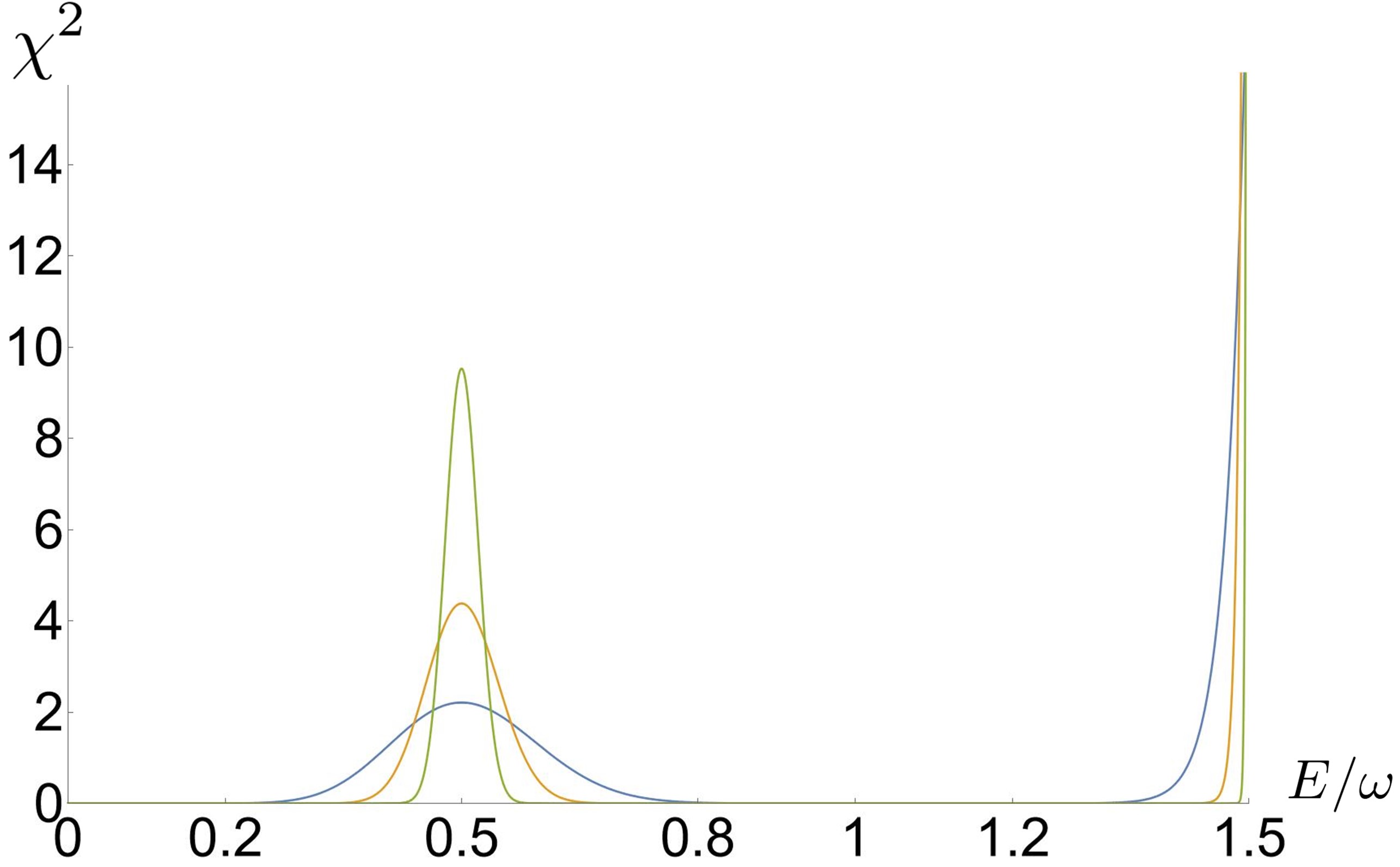
Figure 2: Graphical representation of $\chi^{2}$ when $\kappa rJ=3/4$ for $J=30$ (blue line), $J=120$ (orange line) and $J=570$ (green line).

V A classical magnetic clock for a classical oscillator

In this last section we want to see if the above scheme also works in a completely classical setting, i.e. where we might find connections with general relativity and gravity. To this aim we assume that $\Gamma$ is macroscopic and the theory that describes it fulfills the conditions ensuring the possibility of an effectively equivalent classical description. This is done as in Sec. IV by introducing GCS for $\Gamma$, the usual Glauber coherent states for the harmonic oscillator (HCS), defined as

$$\ket{\alpha}_{{}_{{\Gamma}\,}}=e^{\alpha\hat{\mathsf{a}}-\alpha^{*}\hat{\mathsf{a}}^{\dagger}}\ket{0}_{{}_{{\Gamma}\,}}\mbox{\;with\;}\ket{\alpha}\leftrightarrow\alpha\in\mathbb{C}~{},$$ (36)

where $\mathbb{C}$ is the complex plane. According to Eq. (1) the quantum-to-classical crossover is obtained for $M\to\infty$; moreover, as in the case of the magnetic system, the expectation values of $\hat{H}_{{}_{{\Gamma}\,}}$ upon HCS

$$\braket{\alpha}{\hat{H}_{{}_{{\Gamma}\,}}}{\alpha}=\omega\left(M|\alpha|^{2}+\frac{1}{2}\right)~{}:=E_{{}_{{\Gamma}\,}}(|\alpha|)$$ (37)

must stay finite as $M\to\infty$, and we hence require

$$\lim_{M\to\infty}M\omega<\infty~{}.$$ (38)

Despite Eq. (12) remains well defined in this limit, provided Eq. (31) holds, we notice that quantum numbers, let alone conditions upon them, should have no place in a completely classical description, suggesting that a different analysis must be used to get information about the classical configurations of $C$ and $\Gamma$ that are compatible with the assumptions of the PaW mechanism. At first sight, it might seem impossible to translate conditions set in a genuinely quantum formalism into something which is meaningful also in classical physics. However, one of the most relevant bonuses provided by parametric representations with GCS is that they allow us to move into the classical realm while keeping contact with the original quantum description. In fact, using the resolution of the identity upon ${\cal H}_{{}_{{\Gamma}\,}}$ provided by the HCS, we write Eq. (29) as

$$\ket{\Psi}\!\rangle=\int_{S^{2}}d\mu(\Omega)\int_{\mathbb{C}}d\mu(\alpha)\;\beta(\Omega,\alpha)\ket{\Omega}_{{}_{{C}\,}}\ket{\alpha}_{{}_{{\Gamma}\,}}~{},$$ (39)

where $d\mu(\alpha)=\frac{M}{2\pi}d\alpha d\alpha^{*}$ is the measure on $\mathbb{C}$, and the square modulus of the function

$$\beta(\Omega,\alpha):=\big{(}\,_{{{}_{{C}\,}}\!\!\!}\bra{\Omega}\otimes\,_{{{}_{{\Gamma}\,}}\!\!\!}\bra{\alpha}\big{)}\ket{\Psi}\rangle$$ (40)

is the conditional probability for $\Gamma$ to be in the state $\ket{\alpha}$ when $C$ is in the state $\ket{\Omega}$, or vice-versa, given that the global system $\Psi$ is in $\ket{\Psi}\!\rangle$. Requiring that this probability be finite has the same meaning of Eq. (12). In fact, only the classical configurations of clock and evolving system, defined by the respective phase-space coordinates $\Omega\in S^{2}$ and $\alpha\in\mathbb{C}$, and such that

$$|\beta(\Omega,\alpha)|^{2}>0~{},$$ (41)

are allowed configurations $(\Omega,\alpha)$ of the global system $\Psi$. Using results from, for instance, Ref. Perelomov86 , reminding Eq. (19), $n_{m}:=\kappa r(m+J)-\frac{1}{2}$, and $\Omega=\frac{\theta}{2}\exp^{-i\varphi}$, it is

$$\beta(\Omega;\alpha)=\sum_{m\in\mathcal{A}}c_{m}\braket{\Omega}{J,m}\braket{\alpha}{n_{m}}$$ (42)

$$=\sum_{m\in\mathcal{A}}c_{m}\binom{2J}{m+J}^{1/2}\left(\cos\frac{\theta}{2}\right)^{J-m}\left(\sin\frac{\theta}{2}\right)^{J+m}\cdot$$

$$\qquad\quad\cdot\;e^{-i\varphi(J+m)}\quad e^{-\frac{M|\alpha|^{2}}{2}}\frac{(\sqrt{M}\alpha)^{n_{m}}}{\sqrt{n_{m}!}}$$

$$\!\!\!\!\!\!\!\!\!\!\!\!\!\!\xrightarrow{J,M\rightarrow\infty}\sum_{m\in\mathcal{A}}c_{m}\;\;\delta\left(m+J\cos\theta\right)\,e^{-i\varphi(J+m)}\quad\cdot$$

$$\qquad\qquad\quad\cdot\,\delta\left(M|\alpha|^{2}-n_{m}\right)\;e^{-in_{m}\arg{\alpha}}~{},$$ (43)

and the condition (41) translates into

$$\begin{cases}m=-J\cos\theta\\ M|\alpha|^{2}=n_{m}\sim\kappa r(m+J)~{},\end{cases}$$

where we have neglected $\frac{1}{2}$ w.r.t. $M|\alpha|^{2}$, for $M\to\infty$, i.e

$$\omega M|\alpha|^{2}=\epsilon J(1-\cos\theta)\coloneqq E~{},$$ (44)

which is a perfectly meaningful classical condition. In fact, reminding that $\omega M|\alpha|^{2}=\langle{\alpha|\hat{H}_{{}_{{\Gamma}\,}}|\alpha}\rangle:=E_{{}_{{\Gamma}\,}}(|\alpha|)$ and $\epsilon J(1-\cos\theta)=\langle{\Omega|\hat{H}_{C}|\Omega}\rangle:=E(\theta)$, Eq. (44) tells us that the classical state identified by the representative point $(q,p)$ in the phase-space of $\Gamma$ (see below for the definition of $(q,p)$) is accessible to the system $\Gamma$ at time $t$, as marked by the clock $C$ in the state with representative point $(\theta,\phi)$, only if $\Gamma$ and $C$ have the same energy (we remind that the PaW constraint (5) sets the energy of the whole system, but different combinations of subsystems energies are still allowed).

Indeed, as shown in Ref. FCBCVnat21 , the constraint in Eq. (44) defines a map, that leads to the Hamilton EoM, between points in the $\Gamma$ and $C$ respective phase spaces (the plane and the sphere in this example):

$$\alpha=\sqrt{\frac{E}{M\omega}}\,e^{-i(\eta\,t+\varphi_{0})}~{},$$ (45)

where $\eta,\varphi_{0}\in\mathbb{R}$ and we used the coordinates $(E,t)\in S^{2}$ for identifying points on the sphere, with $E=E(\theta)$ as defined under Eq. (30) and $t=t(\varphi)=\varphi/\epsilon$. In order to describe the classical configurations, we introduce a pair $(q,p)$ of conjugate coordinates for the oscillator by means of the following Darboux chart on the symplectic manifold $\mathbb{C}$

$$\alpha=\sqrt{\frac{M\omega}{2}}\left(q+i\frac{p}{M\omega}\right)~{},$$ (46)

such that $\{q,p\}_{{}_{{\Gamma}\,}}=1$, with $\{\cdot,\cdot\}_{{}_{{\Gamma}\,}}$ Poisson brackets for $\Gamma$, obtained starting from the measure $d\mu(\alpha)$ as in Ref. Perelomov86 . Using the chart (46), Eq. (37) takes the same form of the Hamiltonian function of a unit mass classical harmonic oscillator with frequency $M\omega$, i.e.

$$H_{{}_{{\Gamma}\,}}(q,p)=\frac{p^{2}}{2}+\frac{1}{2}(M\omega)^{2}q^{2}~{},$$ (47)

and the classical configurations, surviving the classical limit according to Eq. (43), look as

$$\Bigg{(}E,t;\;q=\frac{\sqrt{2E}}{M\omega}\cos{\left(\eta\,t+\varphi_{0}\right)},$$

$$\qquad\quad p=-\sqrt{2E}\sin{\left(\eta\,t+\varphi_{0}\right)}\Bigg{)}\in S^{2}\times\mathbb{C}~{},$$ (48)

with

$$E=H_{{}_{{\Gamma}\,}}(q,p)=\omega\left(n+\frac{1}{2}\right)\sim(M\omega)\frac{n}{M}\;\mbox{(for $M\rightarrow\infty$)}$$ (49)

for any $n$ appearing in Eq. (43). It is now easy to verify that the configurations (V) satisfy

$$\begin{dcases}\{p,H_{{}_{{\Gamma}\,}}\}_{{}_{{\Gamma}\,}}=\frac{M\omega}{\eta}\frac{dp}{dt}\\ \{q,H_{{}_{{\Gamma}\,}}\}_{{}_{{\Gamma}\,}}=\frac{M\omega}{\eta}\frac{dq}{dt}\end{dcases}$$ (50)

i.e., the Hamilton equations of motion ruling the classical dynamics of $\Gamma$ where, once the arbitrary constant $\eta$ is set equal to $M\omega$, time is recognized, as for the quantum cases of the previous sections, with the parameter $t=\varphi/\epsilon$ provided by the magnetic clock, and $\mathbb{C}$ plays the role of the $\Gamma$ phase-space. Moreover the clock provides to the oscillator the additional parameter $E$ which identifies the energy of $\Gamma$ which, being $H_{{}_{{\Gamma}\,}}$ time independent, consistently is a constant of motion. Notice that, as a consequence of having started from quantum physics, the energy values appear discretized as in (49), but the difference between any two values consistently tends to $0$ as $M\rightarrow\infty$, i.e. as the $\Gamma$ classical limit is taken.

Let us finally highlight that, being $S_{2}$ a symplectic manifold, it is possible, starting from the measure $d\mu(\Omega)$ as in Ref. Perelomov86 , to introduce also for the clock $C$ Poisson brackets $\{\cdot,\cdot\}_{{}_{{C}\,}}$ which are related to the ones $\{\cdot,\cdot\}_{{}_{{\Gamma}\,}}$ for $\Gamma$ via the pullback by the map  (45). In particular it is $\{E,t\}_{{}_{{C}\,}}=1$ i.e. the pair $(E,t)$ realizes a Darboux chart on $S_{2}$. Therefore the latter can be recognized by the oscillator as a well-defined ”energy-time phase-space” provided by its clock. Energy and time reveal thus to be conjugate coordinates, but not for the evolving system phase-space (which instead is $\mathbb{C}$).

In order to verify the consistency of the above construction, we look at the graphical representations of the marginal probability distribution related to $|\beta|^{2}$ w.r.t. the evolving system phase-space, described by $(q,p)$, w.r.t. the energy-time phase-space, described by $(E,t)$, and w.r.t. the space-time, described by $(q,t)$. General expressions for such distributions are obtained in App. B. We now consider the case $\kappa=3/4$, $r=2/3$, $M=170$ and, in order to have some control over the figures, choose $c_{m}=(1/\sqrt{2})(\delta_{n_{m},M}+\delta_{n_{m},M/2})$ allowing only the two energy values $E=M\omega$ and $E=M\omega/2$. We start from Fig. 3 for the evolving system phase-space: the configurations consistently lie in two circumferences whose radii are fixed by the allowed energy values.

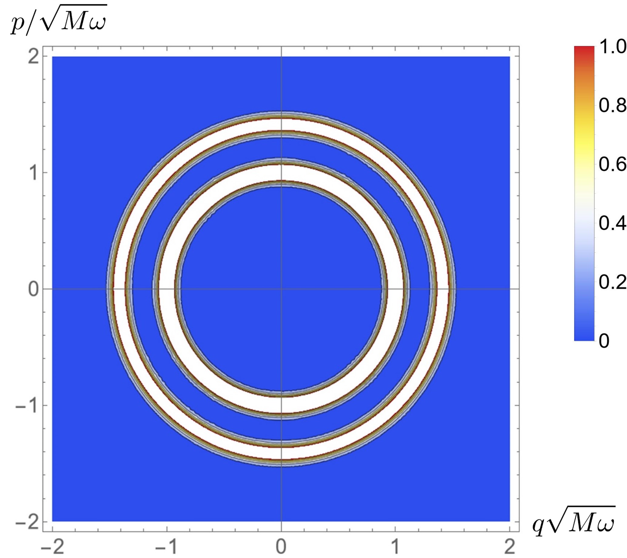
Figure 3: The contour plot of the marginal probability distribution related to $|\beta|^{2}$ w.r.t the evolving system phase-space coordinates for the example with $\kappa=3/4$ introduced in the main text. Considering the dimensionless coordinates defined in the figure, the radii are equal to $\sqrt{2}$ and $1$, for $E=M\omega$ and $E=M\omega/2$, respectively.

As it concerns the energy-time phase-space, the marginal probability distribution in Fig. 4 is, as expected, peaked at any time on $E=M\omega$ and $E=M\omega/2$.

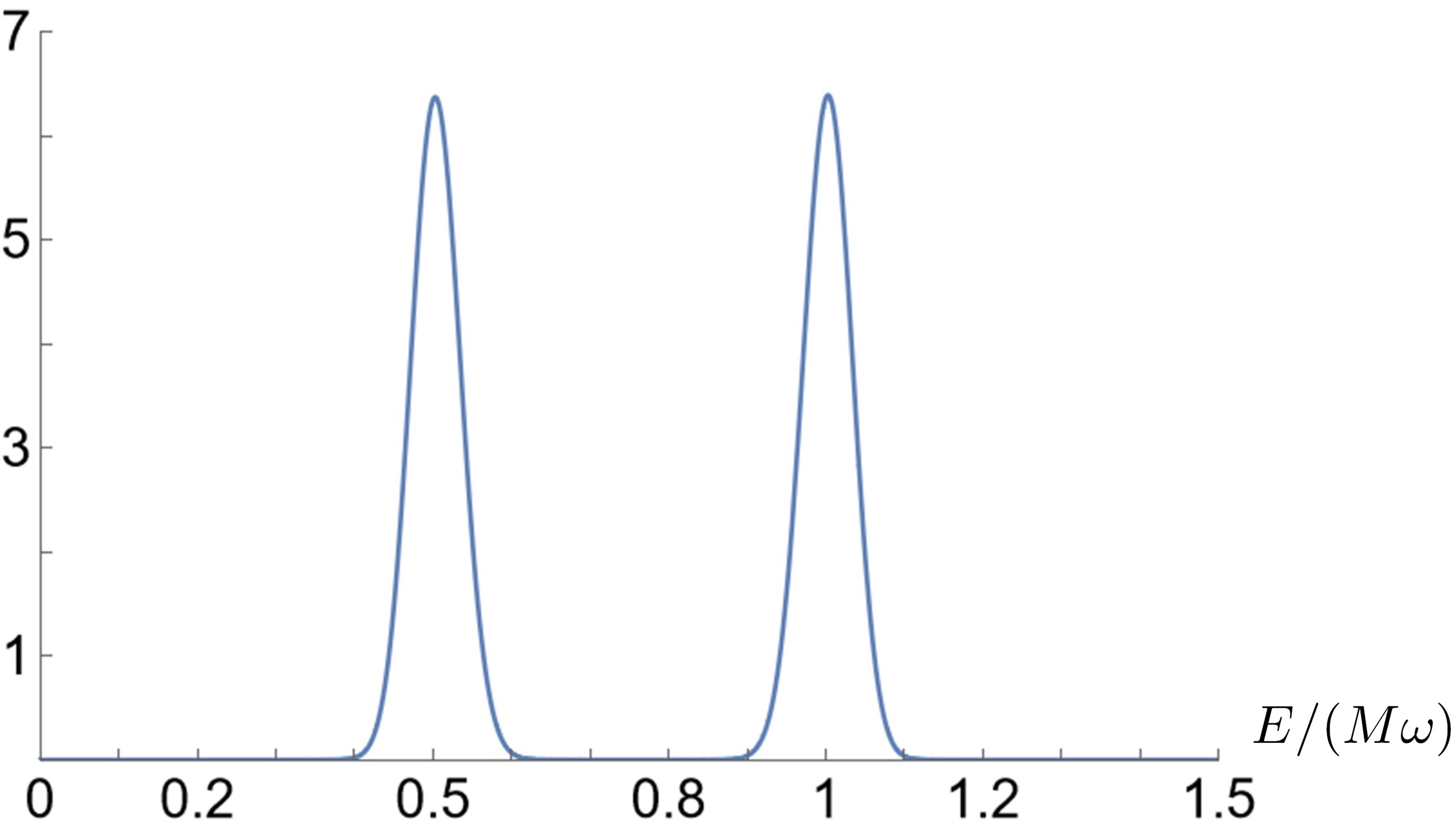
Figure 4: The section at any constant time of the marginal probability distribution related to $|\beta|^{2}$ w.r.t the energy-time phase-space for the example with $\kappa=3/4$ introduced in the main text.

Let us now consider the space-time. It is possible to show, via the properties of the Dirac delta function appearing for $M\rightarrow\infty$ (see App. B), that, as in the panels a) and b) of Fig. 5, the marginal distribution is proportional to $\frac{\Theta(2-Q^{2})}{\sqrt{(2-Q^{2})}}+\frac{\Theta(1-Q^{2})}{\sqrt{(1-Q^{2})}}$ for any time value, with $Q\coloneqq q\sqrt{M\omega}$ and $\Theta$ the Heaviside step function. Consequently the support represented in panel c) of Fig. 5 tends to the region $\mathbb{R}\times[-\sqrt{2},\sqrt{2}]$. Indeed, according the energy values, the maximum value achieved by $Q$ during the time evolution is $\sqrt{2}$. Actually, once the map (45) is introduced, the dynamics emerging from $H_{{}_{{\Gamma}\,}}(q,p)$ takes place just on $\mathbb{R}\times[-\sqrt{2},\sqrt{2}]$. The mentioned dynamics is described by panel d) of Fig. 5 for $E=M\omega$ (red and orange lines) and $E=M\omega/2$ (purple and blue lines), with the initial conditions $q(t=0)=0$ or $q(t=0)=q_{max}$. The latter is the maximum value achieved by the position $q$, therefore $q_{max}=\sqrt{2/(M\omega)}$ for $E=M\omega$ and $q_{max}=\sqrt{1/(M\omega)}$ for $E=M\omega/2$.

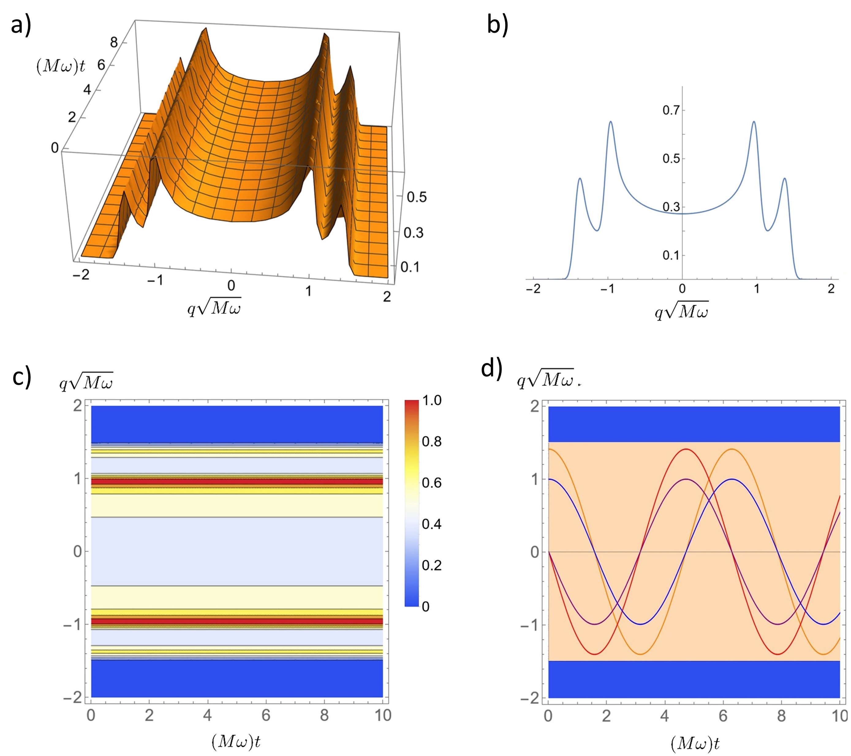
Figure 5: a): Graphical representation of the marginal probability distribution related to $|\beta|^{2}$ w.r.t the space-time coordinates and b) its section at any constant time for the example with $\kappa=3/4$ introduced in the main text. The contour plot of the above distribution is reported in c), while the emergence of the related dynamics, $q$ vs $t$ is reported in d). The light orange region is the support of the marginal probability when $M\rightarrow\infty$.

Let us finally study the case $\kappa=3/4$, $r=2/3$ with every possible state appearing in the decomposition (19). In other words, we assume $c_{m}\neq 0$ for any $m\in\mathcal{A}$ such that $\ket{\Psi}\!\rangle$ is entangled. As we know, the distance between two subsequent energy values tends to $0$ when $M\rightarrow\infty$, therefore the evolving system phase-space and the energy-time one are covered more and more densely by the admitted orbits, as depicted in Figs. 6-7, in accordance with classical physics.

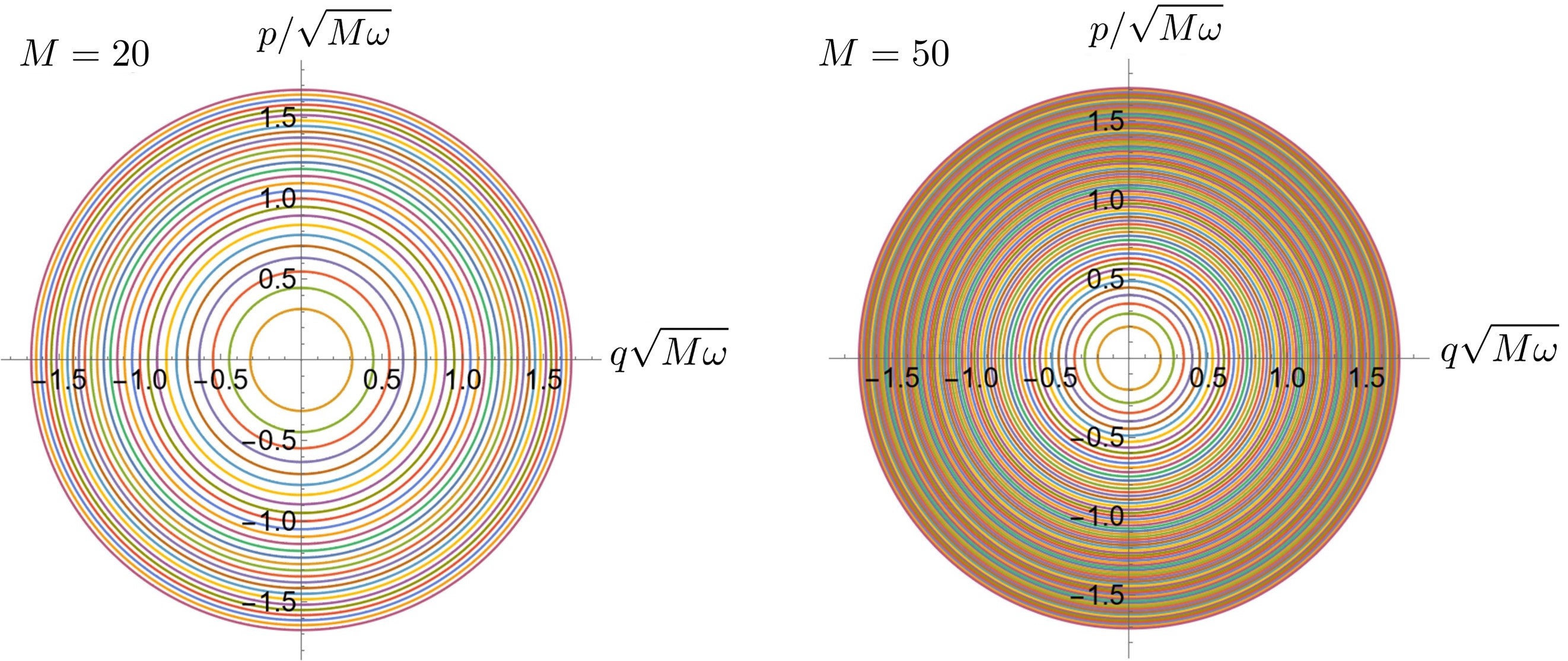
Figure 6: The evolving system phase-space with the admitted orbits when $c_{m}\neq 0$ $\forall m$ and $\kappa=3/4$, $r=2/3$ for $M=20$ (on the left) or $M=50$ (on the right). Using the units in the figure, the orbits are concentric circles with radii $\sqrt{2n/M}$, $n\in\mathbb{N}$. If $M\rightarrow\infty$, the radii are bounded between $0$ and $\sqrt{4\kappa}$.

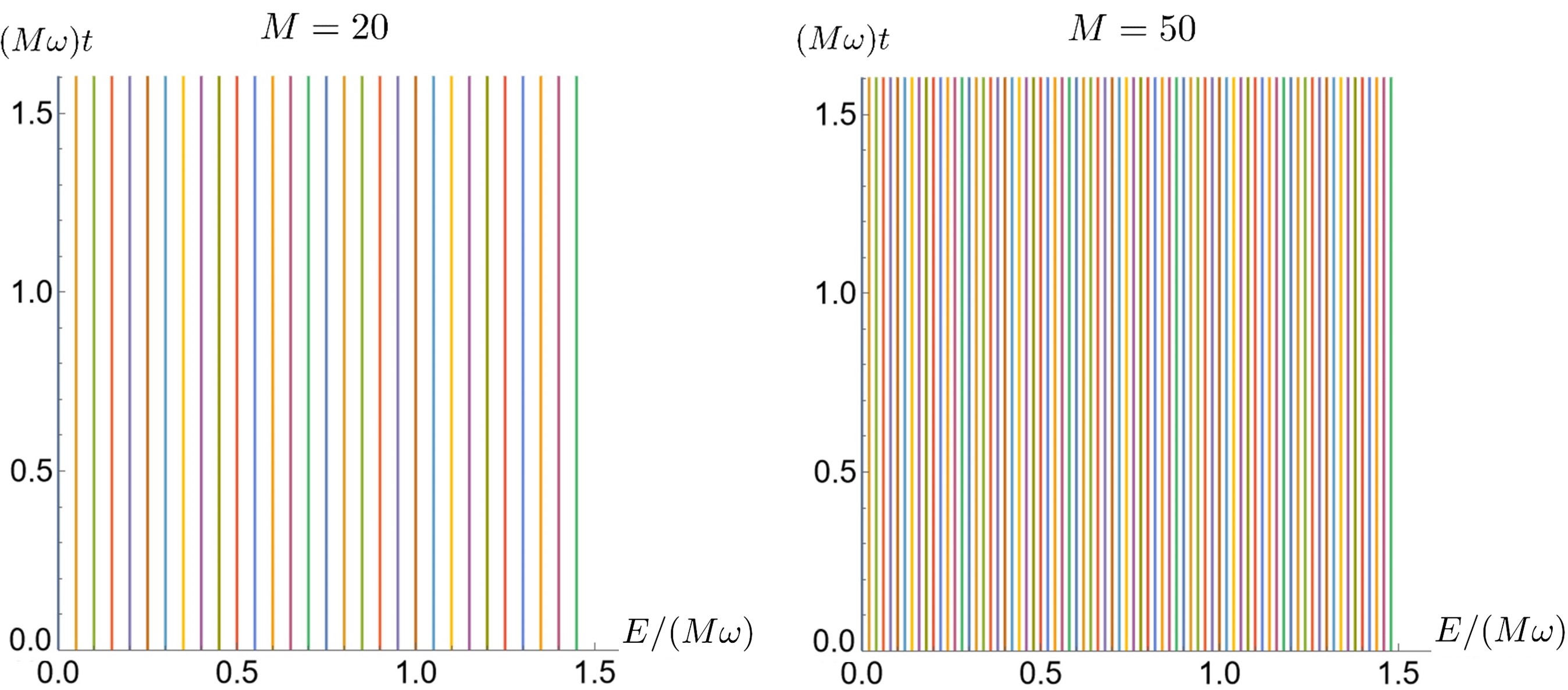
Figure 7: The energy-time phase-space with the admitted orbits when $c_{m}\neq 0$ $\forall m$ and $\kappa=3/4$, $r=2/3$ for $M=20$ (on the left) and $M=50$ (on the right). The orbits are vertical lines satisfying Eq. (49) for $n\in\mathbb{N}$. If $M\rightarrow\infty$, the lines densely populate the region $0<E/(M\omega)<3/2$.

Notice that the phase-spaces are bounded by the maximum energy value $3M\omega/2$. This constraint may sound puzzling as we are used to consider clocks as objects whose capability of marking time is not limited by the evolving system energy. On the other hand it easy to show via Eqs. (12) and (49) that $\kappa\gg 1$, i.e. $J\epsilon\gg M\omega$, is a necessary condition to allow $\Gamma$ to wander in the entire $\mathbb{C}$. The meaning of the above requirement was introduced in the previous section: in order for $C$ to properly work as a clock for $\Gamma$, it must be characterized by a much bigger energy-scale than that of the evolving system, no matter whether this latter is described by a quantum or a classical theory.

DISCUSSION AND CONCLUSIONS

The actual realization of the PaW mechanism we have considered in this paper allows us to bring to light, and improve our understanding of, many facets of the mechanism leading to the definition of time starting from a fully quantum description. In contrast with other implementations of the PaW mechanism discussed in the literature, which consider continuous and unbounded spectra for the clock, and possibly for the system too, our construction is built upon two paradigmatic quantum systems with a discrete spectrum and, for the spin system, even with a separable Hilbert space. As a consequence, as we have shown in full detail in Sec. III, the implementation of the PaW constraint (6) leads to strict conditions on the parameters setting the energy scales of the two systems and on the allowed states appearing in the global entangled state $\ket{\Psi}\!\rangle$, which may limit the capability of the clock to describe the dynamics of the evolving system $\Gamma$ to a rather small subset of its Hilbert space. However, as discussed in Sec. IV, such limitations are removed, and the possibility to describe the full dynamics of $\Gamma$ is recovered, when the macroscopic (classical limit) of the clock-system is taken in order to reconcile the quantum definition of time by the PaW mechanism with the usual classical ”time” variable appearing in the Schrödinger equation. The steps followed in Sec. IV showed that taking the macroscopic limit of the clock $J\to\infty$ is not by itself enough to reach the goal: indeed, this must be accompanied by a proper choice of the energy scale of the clock, that must be large enough to allow the dynamical system to explore its full Hilbert space. The specific conditions expressed in Eqs. (12)-(18), and further specialized in the paragraph around Eq. (35), when the classical limit of the clock is taken, clearly depends on the algebras of the actual models describing the evolving system $\Gamma$ and the clock $C$, but they allowed us to illustrate by a specific example the general property, implied by the PaW mechanism, that it is only the combined effect of the macroscopic limit and of the magnitude of the energy of the clock, that allows us to recover the continuous parameter traditionally employed to follow the evolution of a quantum system $\Gamma$. In the same section, Eqs. (30)-(34), we were also able to show how the parameters defining the GCS state of the clock provide not only the description of the dynamics, but also define the energy of the evolving system, proving once again that the relationship between energy and time originates from the clock, as we already observed in Ref. FCBCVnat21 while discussing the time-energy uncertainty relationship within the framework of the PaW mechanism. The emergence of the classical dynamics when also the evolving system becomes macroscopic, discussed in the last section, also benefits from the possibility given by an actual example of implementation of the PaW mechanism: Indeed, in addition to the definition of proper conjugate coordinates for the evolving system, obeying to the Hamilton’s classical equation of motion, already obtained in Ref. FCBCVnat21 , we had the opportunity to show how the marginal probability distribution defined within the fully quantum framework, naturally blends into the expected classical space-time and phase-space orbits of the dynamical system in the macroscopic, classical limit.

APPENDIX A

The conditions (15)-(18) are obtained starting from Eq. (12) which can be rewritten as $\kappa r=(2n+1)/(2(m+J))$. Therefore, being $n$ and $(m+J)$ natural numbers, it is necessary that, when reduced to the lowest terms, $\kappa r=(2i_{n}+1)/(2i_{m})$ with $i_{n},\,i_{m}\,\in\mathbb{N}$. Moreover, since $2n+1=2(m+J)u=(2i_{n}+1)(m+J)/i_{m}$ has to be an odd number, it must be $m+J=i_{m}(2l+1)$ with $l\in\mathbb{N}$. More precisely, due to the constraint $m+J<2J$, it is $l\leq\lfloor J/i_{m}-1/2\rfloor$ so that $J\geq 3i_{m}/2$ in order to ensure that at least two values of $m$ are allowed. Finally, by means of Eq. (12), we obtain $n=i_{n}(2l+1)+l$.

APPENDIX B

In this appendix we obtain the Marginal Probability Distributions (MPDs) related to $|\beta|^{2}$ represented in the Figs. 3-4-5 of Sec. V.

B.1.   MPD w.r.t. the evolving system phase-space coordinates

The MPD related to $|\beta|^{2}$ w.r.t. the evolving system phase-space, represented in Fig. 3, is obtained from Eq. (42) by means of the resolution of identity given by the GCS on $\mathcal{H}_{{}_{{C}\,}}$, from which

$$\int_{S_{2}}d\mu(\Omega)|\beta|^{2}=\sum_{m\in\mathcal{A}}|c_{m}|^{2}\left|\braket{\alpha}{n_{m}}\right|^{2}~{}.$$ (51)

Considering now the expression of $\braket{\alpha}{n}$ in Ref. Perelomov86 , the measure $d\mu(\alpha)$ below Eq. (39) and the chart (46) on $\mathbb{C}$, Eq. (51) reads

$$\frac{M}{2\pi}\sum_{m\in\mathcal{A}}|c_{m}|^{2}\,e^{-\frac{M}{2}\left(Q^{2}+P^{2}\right)}\,\left(\frac{M}{2}(Q^{2}+P^{2})\right)^{n_{m}}\frac{1}{(n_{m})!}$$

$$\xrightarrow{M\rightarrow\infty}\frac{1}{\pi}\sum_{m\in\mathcal{A}}|c_{m}|^{2}\,\delta\!\left(Q^{2}+P^{2}-2n_{m}/M\right)~{},$$ (52)

with $Q\coloneqq q\sqrt{M\omega}$ and $P\coloneqq p/\sqrt{M\omega}$. Finally, for $M\rightarrow\infty$, the configurations lie in circumferences with radii $2n/M=E/(M\omega)$, where the last equality follows from Eq. (49).

B.2.   MPD w.r.t. energy-time variables

The MPD related to $|\beta|^{2}$ w.r.t. the energy-time phase-space, represented in Fig. 4, is obtained from Eq. (42) by means of the resolution of identity given by the GCS on $\mathcal{H}_{{}_{{\Gamma}\,}}$, from which

$$\int_{\mathbb{C}}d\mu(\alpha)|\beta|^{2}=\sum_{m\in\mathcal{A}}|c_{m}|^{2}\left|\braket{\Omega}{J,m}\right|^{2}=\chi^{2}(\theta)~{},$$ (53)

as defined in Eq. (25). Therefore, defining $\mathtt{e}\coloneqq E/(M\omega)$, considering Eqs. (26) and (30) together with the measure $d\mu(\Omega)$ below (29), Eq. (53) reads

$$\chi^{2}(\mathtt{e}) =\frac{2J+1}{2\kappa}\sum_{m\in\mathcal{A}}|c_{m}|^{2}\binom{2J}{m+J}\left(1-\frac{\mathtt{e}}{2\kappa}\right)^{J-m}\left(\frac{\mathtt{e}}{2\kappa}\right)^{J+m}$$

$$\xrightarrow{J\rightarrow\infty}\sum_{m\in\mathcal{A}}|c_{m}|^{2}\delta\left(\mathtt{e}-\kappa(1+m/J)\right)$$

$$=\sum_{m\in\mathcal{A}}|c_{m}|^{2}\delta\left(\mathtt{e}-n_{m}/M\right)~{},$$ (54)

where we used Eq. (12).

B.3.   MPD w.r.t. the space-time coordinates

The MPD related to $|\beta|^{2}$ w.r.t. the space-time is

$$\left(\frac{2J+1}{2\kappa}\int_{0}^{3/2}d\mathtt{e}\right)\;\left(\frac{M}{2\pi}\int_{-\infty}^{+\infty}dP\right)\,|\beta|^{2}$$ (55)

with $\mathtt{e}\coloneqq E/(M\omega)$ and $P\coloneqq p/\sqrt{M\omega}$. In order to have some control over the calculation, let us assume that, as in the example of the main text, $\mathrm{dim}(\mathcal{H}_{{}_{{\Gamma}\,}})=2$, i.e. that only two couples $(m_{i},n_{i}\coloneqq n_{m_{i}})$ $i=1,2$ are allowed by Eq. (42). Moreover let us write $\beta=c_{1}z_{1}+c_{2}z_{2}$ where $c_{i}\coloneqq c_{m_{i}}$, $z_{i}\coloneqq z_{i}^{{}_{{C}\,}}z_{i}^{{}_{{\Gamma}\,}}$ and $z_{i}^{{}_{{C}\,}}\coloneqq\braket{\Omega}{J,m_{i}}$, $z_{i}^{{}_{{\Gamma}\,}}\coloneqq\braket{\alpha}{n_{i}}$. Once implemented, the changes of coordinates $(\theta,\varphi)\Rightarrow(\mathtt{e},t)$ for $S_{2}$ and $\alpha\Rightarrow(P,Q)$ for $\mathbb{C}$ with $t\coloneqq\varphi/\epsilon$ and $Q\coloneqq q\sqrt{M\omega}$, we decompose Eq. (55) as the sum of three integrals $I_{1}+I_{2}+I_{int}$ defined via

$$\!\begin{cases}I_{i}\coloneqq|c_{i}|^{2}\;\cdot\;\left(\frac{2J+1}{2\kappa}\int_{0}^{3/2}d\mathtt{e}\,|z_{i}^{{}_{{C}\,}}|^{2}\right)\;\cdot\;\left(\frac{M}{2\pi}\int_{-\infty}^{+\infty}dP\,|z_{i}^{{}_{{\Gamma}\,}}|^{2}\right)\vspace*{1mm}\\ \,\,\quad=|c_{i}|^{2}\;\cdot\;\frac{M}{2\pi}\int_{-\infty}^{+\infty}dP\,|z_{i}^{{}_{{\Gamma}\,}}|^{2}\\ \\ I_{int}\coloneqq 2|c_{1}|\,|c_{2}|\;\cdot\;\left(\frac{2J+1}{2\kappa}\int_{0}^{3/2}d\mathtt{e}\,|z_{1}^{{}_{{C}\,}}|\,|z_{2}^{{}_{{C}\,}}|\right)\;\cdot\\ \qquad\quad\cdot\left(\frac{M}{2\pi}\int_{-\infty}^{+\infty}dP\,|z_{1}^{{}_{{\Gamma}\,}}|\,|z_{2}^{{}_{{\Gamma}\,}}|\,\cos(z_{int})\right)\end{cases}$$ (56)

where $z_{int}\coloneqq(n_{1}-n_{2})\arctan(P,Q)+(m_{1}-m_{2})\varphi+\arg(c_{1})-\arg(c_{2})$. Considering now the limits $J,M\rightarrow\infty$, $I_{i}$ can be evaluated via

$$I_{i}\xrightarrow{N\rightarrow\infty}\frac{|c_{i}|^{2}}{\pi}\;\cdot\;\int_{-\infty}^{+\infty}dP\,\delta\!\left(Q^{2}+P^{2}-2n_{i}/M\right)$$

$$=\frac{2|c_{i}|^{2}\;\Theta\left(2n_{i}/M-Q^{2}\right)}{\pi}\;\cdot\;\int_{0}^{+\infty}\frac{dP}{|2P|}$$

$$\left[\delta\left(P-\sqrt{2n_{i}/M-Q^{2}}\right)+\delta\left(P+\sqrt{2n_{i}/M-Q^{2}}\right)\right]$$

$$=|c_{i}|^{2}\;\frac{\Theta\left(2n_{i}/M-Q^{2}\right)}{\pi\sqrt{2n_{i}/M-Q^{2}}}$$ (57)

with $\Theta$ the Heaviside step function. As concerns $I_{int}$, the integral in $d\mathtt{e}$ can be exactly calculated as

$$\binom{2J}{m_{1}+J}^{1/2}\binom{2J}{m_{2}+J}^{1/2}\binom{2J}{\frac{m_{1}+m_{2}}{2}+J}^{-1}\xrightarrow{J\rightarrow\infty}0$$ (58)

for $m_{1}\neq m_{2}$, instead the integral in $dP$ can be approximated for $M\rightarrow\infty$ as

$$\frac{\big{(}(n_{1}+n_{2})/2\big{)}!}{\sqrt{n_{1}!n_{2}!}}\,\cdot\,\frac{\Theta\left((n_{1}+n_{2})/M-Q^{2}\right)}{\pi\sqrt{(n_{1}+n_{2})/M-Q^{2}}}\,\cdot$$

$$\cdot\left(\cos[...]+\cos[...]\right)\xrightarrow{M\rightarrow\infty}0$$ (59)

for $n_{1}\neq n_{2}$, with the factorial extended using the Euler Gamma-function when necessary and where, according to Eqs. (12)-(13), we assumed $n_{1},n_{2}\propto M$ and $m_{1},m_{2}\propto J$. Finally, in the classical limit, $I_{int}\rightarrow 0$ and Eq. (55) reads

$$\sum_{m\in\mathcal{A}}|c_{m}|^{2}\,\frac{\Theta\left(2n_{m}/M-Q^{2}\right)}{\pi\sqrt{2n_{m}/M-Q^{2}}}~{}.$$ (60)

References

- [1] P. A. M. Dirac, P. A. M Dirac, and P. A. M Dirac. The principles of quantum mechanics. / by P.A.M. Dirac. The international series of monographs on physics 27. Clarendon Press, Oxford, 4th ed. edition, 1958.
- [2] A. Peres. Quantum Theory: Concepts and Methods. Kluwer, Dordrecht, 2002.
- [3] Í.L. Egusquiza J.G. Muga, R. Sala Mayato. Time in Quantum Mechanics. Springer Verlag - Berlin Heidelberg, 2002.
- [4] D. Page and K. Wootters. Evolution without evolution: dynamics described by stationary observables. Phys. Rev. D, 27:2885–2892, 1983.
- [5] V. Giovannetti, S. Lloyd, and L. Maccone. Quantum time. Phys. Rev. D, 92:045033, 2015.
- [6] C. Marletto and V. Vedral. Gravitationally induced entanglement between two massive particles is sufficient evidence of quantum effects in gravity. Phys. Rev. Lett., 119:240402, Dec 2017.
- [7] K. L. H. Bryan and A. J. M. Medved. Realistic clocks for a universe without time. Foundations of Physics, 48:48–59, 2018.
- [8] A, R. H. Smith and M. Ahmadi. Quantizing time: Interacting clocks and systems. Quantum, 3:160, July 2019.
- [9] M. Basil Altaie, D. Hodgson, and A. Beige. Time and quantum clocks: A review of recent developments. Frontiers in Physics, 10, 2022.
- [10] E. Castro-Ruiz, F. Giacomini, A. Belenchia, and C. Brukner. Quantum clocks and the temporal localisability of events in the presence of gravitating quantum systems. Nature Communications, 11(1):2672, May 2020.
- [11] V. Baumann, M. Krumm, P. A. Guérin, and C. Brukner. Noncausal page-wootters circuits. Phys. Rev. Res., 4:013180, Mar 2022.
- [12] C. Rovelli. Relational quantum mechanics. International Journal of Theoretical Physics, 35(8):1637–1678, Aug 1996.
- [13] L. Chataignier. Relational observables, reference frames, and conditional probabilities. Phys. Rev. D, 103:026013, Jan 2021.
- [14] C. Foti, A. Coppo, G. Barni, A. Cuccoli, and P. Verrucchi. Time and classical equations of motion from quantum entanglement via the Page and Wootters mechanism with generalized coherent states. Nat. Commun., 12:1787, 2021.
- [15] A.M. Perelomov. Generalized Coherent States and Their Applications. Springer-Verlag, 1986.
- [16] M. A. C. Rossi, C. Foti, A. Cuccoli, J. Trapani, P. Verrucchi, and M. G. A. Paris. Effective description of the short-time dynamics in open quantum systems. Phys. Rev. A, 96:032116, Sep 2017.
- [17] A. Coppo, A. Cuccoli, C. Foti, and P. Verrucchi. From a quantum theory to a classical one. Soft Computing, 24:10315, 2020.
- [18] M. Born and R Oppenheimer. Zur quantentheorie der molekeln. Annalen der Physik, 389:457, 1927.
- [19] G. Hunter. Conditional probability amplitudes in wave mechanics. Int. J. Quantum Chem., 9:237, 1975.
- [20] D. Calvani, A. Cuccoli, N. I. Gidopoulos, and P. Verrucchi. Parametric representation of open quantum systems and cross-over from quantum to classical environment. PNAS, 110(17):6748–6753, 2013.
- [21] P. Liuzzo-Scorpo, A. Cuccoli, and P. Verrucchi. Parametric description of the quantum measurement process. EPL (Europhysics Letters), 111(4):40008, 2015.
- [22] P. Liuzzo-Scorpo, A. Cuccoli, and P. Verrucchi. Getting information via a quantum measurement: The role of decoherence. International Journal of Theoretical Physics, 54(12):4356–4366, 2015.
- [23] L.G. Yaffe. Large N limits as classical mechanics. Rev. Mod. Phys., 54:407, 1982.
- [24] A. Coppo., N. Pranzini, and P. Verrucchi. Threshold size for the emergence of classical-like behavior. Phys. Rev. A, 106:042208, 2022.