On Data-Driven Surrogate Modeling for Nonlinear Optimal Control

Abstract

In this paper, we study the use of state-of-the-art nonlinear system identification techniques for the optimal control of nonlinear systems. We show that the nonlinear systems identification problem is equivalent to estimating the generalized moments of an underlying sampling distribution and is bound to suffer from ill-conditioning and variance when approximating a system to high order, requiring samples combinatorial-exponential in the order of the approximation, i.e., the global nature of the approximation. We show that the iterative identification of “local” linear time varying (LTV) models around the current estimate of the optimal trajectory, coupled with a suitable optimal control algorithm such as iterative LQR (ILQR), is necessary as well as sufficient, to accurately solve the underlying optimal control problem.

I Introduction

Many physical systems are analytically intractable (Fig. 1). Thus, in order to devise strategies for optimal control of such systems, there is a need for accurate identification of the dynamics of these systems. This is especially attractive in scenarios where utilization of a ‘black-box’ computational model is expensive, and thus, a simplified ‘surrogate’ model identified from the original dynamics can be used to replace the actual system. In this paper, we study the use of data-based approach, as in supervised learning, to generate these surrogate models. We explore the performance of two representative nonlinear system identification techniques, a recent linear in parameters approximator SINDy [1], and the nonlinear in parameters deep neural-networks, and give a theoretical explanation, as well as empirical evidence, for the issues of ill-conditioning and variance that affect the performance of such nonlinear identification techniques. Moreover, we show that, to combat these issues with the “global” nonlinear models, in order to solve the underlying optimal control problem, the iterative identification of “local” linear time varying (LTV) models around the current estimate of the optimal trajectory, coupled with a suitable optimal control algorithm such as iterative LQR (ILQR) [2], is necessary as well as sufficient.

((a))

((b))

Figure 1: In many scenarios, the dynamics of the physical systems are generally analytically unknown, and we only can access an input-output computational ‘black box’. In the swimmer examples above, the fluid-structure interactions lead to analytically unknown equations.

Nonlinear system identification has a wide variety of methods developed, such as block-oriented structures [3][4], nonlinear state-space representations [5][6], nonlinear autoregressive exogeneous (NARX) and nonlinear autoregressive moving average with exogenous input (NARMAX) models [7], and piecewise linear models [8], as some examples. More recent work includes SINDy, a data-driven algorithm which utilizes nonlinear basis functions for the functional approximation of the unknown nonlinear dynamics, through a least-squares regression. Well-known nonlinear function approximators such as deep neural networks, RNNs and LSTMs [9][10][11] have also been used to approximate the dynamics, in a similar fashion to NARX models. While all these techniques have their own merits and de-merits, none have managed to satisfactorily resolve the central issue with nonlinear identification problems [12][13], namely that of data inadequacy [14]. In this paper, we show that these techniques require a large amount of data to accurately estimate model parameters, with the required amount of data scaling in an exponential-combinatorial fashion with increase in the model complexity. This is especially apparent in continuous state-space systems, wherein capturing all parts of the underlying dynamics is intractable, making the models poorly generalize and/ or overfit. This, consequently, leads to issues dealing with validation and generalization of the models [15], since assessing the generalization performance and the robustness of these models is a challenge. Another major challenge that is especially prevalent in neural-network based techniques is the physical interpretability, or the lack thereof, for these models [16]. For linear function approximation techniques such as SINDy, which operate with user-specified nonlinear basis functions, the selection of the basis is crucial, and thus, finding the correct model structure selection remains a challenge [14].

The basic problem of controlling nonlinear systems is very challenging. Despite a rich history of control technqiues for nonlinear dynamical systems, the area of data-driven optimal controls is still a topic of active research and called Reinforcement Learning [17][18][19]. In our previous work [20][21], we proposed a data-based algorithm for optimal nonlinear control, which identifies successive LTV models combined with the so-called ILQR approach to yield a globally optimum local feedback law and is far more efficient, reliable and accurate when compared to state of the art RL techniques [20]. The ILQR algorithm [22] is a sequential quadratic programming (SQP) approach, for the solution of optimal control problems, and under relatively mild conditions can be shown to converge to the global minimum of the optimal control problem [20].

In this paper, we use deep neural-networks as a representative nonlinear (in parameters), and SINDy as a linear (in parameters) function approximator, in order to identify the dynamics of nonlinear computational ‘black-box’ models. The primary contributions of this work are as follows: 1) we show that a nonlinear system identification problem is equivalent to a generalized moment estimation problem of an underlying sampling distribution, and thus, when approximating a system to high order, is bound to suffer from ill-conditioning as well as variance, that scales in a combinatorial-exponential fashion; 2) extensive empirical evidence is provided to support the theory showing that the Gram matrix $\mathcal{G}$ is highly ill-conditioned while there is high variance in the forcing function $F$ in the underlying Normal equation $\mathcal{G}C=F$ leading to large errors in the identification of the co-efficients $C$; and 3) moreover, in the context of the motivating problem of solving nonlinear optimal control problems, we show that the use of a ‘local’ LTV approach, as opposed to ‘global’ nonlinear surrogate models as above, is sufficient, as well as necessary, to address the issues of ill conditioning and variance, assuring accurate and provably optimum answers.

The rest of the paper is organized as follows: In Section II, we introduce the nonlinear optimal control problem, and consequently the nonlinear system-identification problem that follows naturally. We discuss the issues related to the use of these techniques in a data-based fashion, and provide theoretical justifications for the same, in Section III. In Section IV, we provide empirical evidence of our proposed theory, wherein we benchmark the ‘global’ surrogate-models learned by the algorithms, and their performance on optimal control computation as compared to a ‘local’ linear time-varying approach.

II Preliminaries

Consider the discrete-time nonlinear dynamical system:

$$x_{t+1}=f(x_{t},u_{t}),$$ (1)

where $x_{t}\in\mathbb{R}^{n_{x}}$ and $u_{t}\in\mathbb{R}^{n_{u}}$ correspond to the state and control vectors at time $t$. The optimal control problem is to find the optimal control policy $\pi^{0}=\{\pi^{0}_{0},\pi^{0}_{1}...\pi^{0}_{T-1}\}$, that minimizes the cumulative cost:

$$\min_{\pi}J^{\pi}(x)=\sum_{t=0}^{T-1}c_{t}(x_{t},u_{t})+c_{T}(x_{T}),$$

subject to the dynamics above, given some $x_{0}=x$, and where $u_{t}=\pi_{t}^{0}(x_{t})$, $c_{t}(\cdot)$ is the instantaneous cost function and $c_{T}(\cdot)$ is the terminal cost. We assume the incremental cost to be quadratic in control, such that $c_{t}(x_{t},u_{t})=l_{t}(x_{t})+\frac{1}{2}u_{t}^{T}Ru_{t}$.

In this work, we consider dynamics that are analytically intractable, i.e., there is no closed-form analytical expression available for the dynamics. Thus, we only have access to the input-output model of the dynamical system, wherein given the inputs $x$ and $u$, a black-box (computational) model generates the next state $x^{\prime}=f(x,u)$.

We consider approaches that may be used to “identify” the nonlinear dynamic model given the input-output black-box model. For instance, these may be linear approximation architectures like SINDy, or nonlinear architectures such as (deep) neural networks. The “hope” is to be able to train these models with the input-output data from the original black-box such that after training, we can obtain a cheap surrogate model to do the optimal control of the system.

For optimal control, we utilize the Iterative Linear Quadratic Regulator (ILQR) algorithm, which can be guaranteed to converge to the global optimum [20]. A brief description of the ILQR Algorithm is given below.

II-A Iterative Linear Quadratic Regulator (ILQR)

The ILQR Algorithm [22] iteratively solves the nonlinear optimal control problem posed in Section II using the following steps:

II-A1 Forward Pass

Given a nominal control sequence $\{u_{t}\}_{t=0}^{T-1}$ and initial state vector $x_{0}$, the state is propagated in time in accordance with the dynamics. $x_{t+1}=f(x_{t},u_{t})$.Thus, we get the nominal trajectory $(\bar{x}_{t},\bar{u}_{t})$ and the linearized system around the nominal: $\delta x_{t+1}=A_{t}\delta x_{t}+B_{t}\delta u_{t}$

II-A2 Backward pass

Using the linearized system, the ILQR algorithm computes a local optimal control by solving the following discrete time Riccati Equation, which is given by,

$$\delta u_{t} =R^{-1}B_{t}^{T}(-v_{t+1}-V_{t+1}(A_{t}\delta x_{t}+B_{t}\delta u_{t}))-\bar{u}_{t},$$

$$=-(R+B^{T}_{t}V_{t+1}B_{t})^{-1}(R\bar{u}_{t}+B_{t}^{T}v_{t+1}$$

$$+B_{t}^{T}V_{t+1}A_{t}\delta x_{t}),$$ (2)

which can be written in the linear feedback form $\delta u_{t}=-k_{t}-K_{t}\delta x_{t}$, where $k_{t}=(R+B_{t}^{T}V_{t+1}B_{t})^{-1}(R\bar{u}_{t}+B_{t}^{T}v_{t+1})$ and $K_{t}=(R+B_{t}^{T}V_{t+1}B_{t})^{-1}B^{T}_{t}V_{t+1}A_{t}$, with

$$v_{t} =l_{t,x}+A_{t}^{T}v_{t+1}-A_{t}^{T}V_{t+1}B_{t}(R+B_{t}^{T}V_{t+1}B_{t})^{-1}$$

$$\cdot(B_{t}^{T}v_{t+1}+R\bar{u}_{t})$$ (3a)

$$V_{t} =l_{t,xx}+A_{t}^{T}(V_{t+1}^{-1}+B_{t}R^{-1}B_{t}^{T})^{-1}A_{t}$$

$$=l_{t,xx}+A_{t}^{T}V_{t+1}A_{t}-A_{t}^{T}V_{t+1}B_{t}(R+B_{t}^{T}V_{t+1}B_{t})^{-1}$$

$$\cdot B_{t}^{T}V_{t+1}A_{t}.$$ (3b)

with the terminal conditions $v_{T}(x_{T})=\frac{\partial c_{T}}{\partial x}|_{x_{T}}=\frac{\partial l}{\partial x}|_{x_{T}}$ and $V_{T}(x_{T})=\nabla^{2}_{xx}c_{T}|_{x_{T}}$. To compute $v_{t}$ and $V_{t}$, we need their corresponding values in the future, i.e. $v_{t+1}$ and $V_{t+1}$. From Eqs. 3a and 3 we see that, given the terminal conditions and the local LTV model parameters $(A_{t},B_{t})$, we can do a backward-in-time sweep to compute all values of $v_{t}$ and $V_{t}$, and thus, the corresponding optimal control for that trajectory.

II-A3 Update trajectory

Now, given the gains from the backward pass, we can update the nominal control sequence as $\bar{u}_{t}^{k+1}=\bar{u}_{t}^{k}+k_{t}+K_{t}(x_{t}^{k+1}-x_{t}^{k})$, and $x^{k+1}_{0}=x^{k}_{0}$. If the convergence criteria is not met ($k_{t}\approx 0$), we iterate the process by repeating steps (1) to (4).

II-B Approximation Problem

Let $f:\mathbb{R}\rightarrow\mathbb{R}$ be a function, and $p(\cdot)$ be a p.d.f./sampling distribution on $\mathbb{R}$. The inner product w.r.t. the distribution $p(\cdot)$ is defined as $<f,g>=\int_{-\infty}^{\infty}f(x)g(x)p(x)dx$.

We are interested in approximating the function $f(\cdot)$ using a suitable architecture. For simplicity, we consider a scalar, control-free dynamical model $f(\cdot)$. Nonetheless, the results are generalized in a relatively straightforward fashion, while the issues inherent in the Approximation problem come into sharp focus.

Linear

Given a set of basis functions $\{\psi_{1}...\psi_{n}\}$, we want to approximate $f$ in the subspace spanned by $\Psi=span\{\psi_{1}...\psi_{n}\}$, i.e., we want to find $f^{*}=\sum_{i=1}^{n}c_{i}^{*}\psi_{i}$, such that $||f-f^{*}||$ is minimized, where $||f||=\sqrt{<f,f>}$ is the norm induced by the $p(.)$ weighted inner product above.

Nonlinear

Given a nonlinear approximation architecture $h(x,\theta)$, such as a (deep) neural network, we want to find the best approximation of $f$ in the approximation architecture, i.e. find $f^{*}=h(x,\theta^{*})$ such that $||f-f^{*}||^{2}$ is minimized over all parameters $\theta\in\Theta\subseteq\Re^{n}$.

We can get the answer to the linear question from the Projection Theorem in the Hilbert space $L_{2}(p)$.

The optimal $f^{*}$ is such that $(f-f^{*})\perp\psi_{i}\forall i=1,2...n$, owing to the Projection Theorem. Substituting $f^{*}=\sum_{i=1}^{n}c_{i}^{*}\psi_{i}$ leads to the Normal equations:

$$\mathcal{G}c^{*}=F\\ \implies c^{*}=\mathcal{G}^{-1}F$$ (4)

where $\mathcal{G}_{ij}=<\psi_{i},\psi_{j}>$, $F_{i}=<f,\psi_{i}>$, $i,j=1,2\cdots n$. This result implies that there exists a unique $f^{*}$ such that $||f-f^{*}||$ is minimized, given a linear approximation architecture, owing to the invertibility of $\mathcal{G}$ stemming from the linear independence of the basis $\{\psi_{i}\}$.

Given the nonlinear approximation architecture, one has to solve the least-squares problem $\theta^{*}=\min_{\theta}||f-h(x,\theta)||^{2}$. This may be solved using a suitable optimization algorithm such as gradient descent. Let $J(\theta)=||f-h(x,\theta)||^{2}=\int(f-h(x,\theta))^{2}p(x)dx$. This implies that $\frac{\partial J}{\partial\theta}=-2\int(f-h(x,\theta))h_{\theta}(x,\theta)p(x)dx$, where $h_{\theta}(x,\theta)=\frac{\partial h(x,\theta)}{\partial\theta}$.

Then, we can set up the gradient descent recursion $\theta_{t+1}=\theta_{t}-\gamma\frac{\partial J}{\partial\theta}\Bigg{|}_{\theta_{t}}$, where $\theta_{t}\rightarrow\theta^{*}$ s.t. $\frac{\partial J}{\partial\theta}|_{\theta^{*}}=0$, given a sufficiently small $\gamma$. Note, however, that, unlike the linear case, there is no guarantee that the algorithm converges to the global minimum. Moreover, for a local minimum $\theta^{*}$, $<\Delta^{*},H_{k}^{*}>=0$, for all $k=1,2\cdots n$, where $\Delta^{*}(x)=(f(x)-h(x,\theta^{*}),$ and $H^{*}_{k}=\frac{\partial h}{\partial\theta_{k}}|_{\theta^{*}}$, owing to the necessary condition above, analogous to the Projection Theorem in the linear case.

III Data Driven Solutions

In this section, we assume that we have access only to the data-points $(x^{i},f(x^{i})),i=1,2...R$, where the samples are drawn from the sampling distribution, $x^{i}\sim p(\cdot)$, independently.

III-A Heuristic Idea

In the following, we shall show that approximating $f(\cdot)$ globally, equivalently, to a high polynomial order, is the same as finding the generalized higher order moments of the state $x$, under the sampling density $p(\cdot)$. In particular, the elements of the Gram matrix $\mathcal{G}_{ij}$ are moments of the underlying state: $\mathcal{G}_{11}$ corresponds to the first moment while $\mathcal{G}_{nn}$ corresponds to the $2n^{th}$ moment, and thereby, $\mathcal{G}_{11}\ll\mathcal{G}_{nn}$, leading to severe ill-conditioning of the Gram matrix. Further, $<f,\psi_{n}>$ is the $2n^{th}$ order moment of the state $x$, and thus, its variance is the $4n^{th}$ order moment. Noting that moments grow combinatorially-exponentially in the order of the approximation, for instance, for Gaussian random variables, they grow as $(2n)!!\sigma^{2n}$, where $\sigma^{2}$ is the variance of the underlying sampling density, this implies that the number of samples required to get reliable estimates of the projections grows in a combinatorial-exponential fashion. Thus, the right hand side of the Normal equation $\mathcal{G}C=F$ has high variance while the Gram matrix is ill-conditioned and has high variance, and thus, the solution is bound to be subject to large errors. Moreover, owing to the same reason, there is a lack of convergence of such models, i.e, different datasets lead to different models when approximating to a high order. Further, it is not clear what the sampling distribution ought to be. Thus, in order to combat these issues with estimating nonlinear “global” models, to solve nonlinear optimal control problems, it is necessary and sufficient that we identify local LTV systems by sampling “locally” around our current estimate of the optimal control trajectory and iterating till convergence as in the ILQR approach.

III-B Linear Case

Given the sample set $(x^{i},f(x^{i}))$, let:

$$f(x^{j})\approx\sum_{i=1}^{n}c_{i}\psi_{i}(x^{j})~{}\forall~{}j=1,2...R.$$ (5)

We can collate the equations and represent the problem as $\underline{\Psi}^{R}\bar{C}^{R}\approx F^{R}$ where $\underline{\Psi}^{R}_{ik}=\psi_{i}(x^{k})$ $F^{R}_{k}=f(x^{k})$, where $i=1,2\cdots n$ and $k=1,2\cdots R$. The solution to Eq. 5 is given by the Least-Squares approach that minimizes the error between the two sides of the equation:

$$\bar{C}^{R}=(\underline{\Psi}^{R^{\prime}}\underline{\Psi}^{R})^{-1}\underline{\Psi}^{R^{\prime}}F^{R}.$$ (6)

It is now politic to look at the terms $\underline{\Psi}^{R^{\prime}}\underline{\Psi}^{R}$ and $\underline{\Psi}^{R^{\prime}}F^{R}$. After expansion, $(\underline{\Psi}^{R^{\prime}}\underline{\Psi}^{R})_{ij}=\sum_{k=1}^{R}\psi_{i}(x^{k})\psi_{j}(x^{k})$, and $(\underline{\Psi}^{R^{\prime}}F^{R})_{i}=\sum_{k=1}^{R}\psi_{i}(x^{k})f(x^{k})$.

Note that the samples $x^{i}\sim p(\cdot)$. We can write the equations $\frac{1}{R}\sum_{i=1}^{R}\psi_{k}(x^{i})\psi_{l}(x^{i})\rightarrow\int\psi_{k}(x)\psi_{l}(x)p(x)dx=<\psi_{k},\psi_{l}>$, and $\frac{1}{R}\sum_{i=1}^{R}\psi_{k}(x^{i})f(x^{i})\rightarrow\int\psi_{k}(x)f(x)p(x)dx=<\psi_{k},f>$, as $R\rightarrow\infty$, owing to the Law of Large Numbers. This implies that $\bar{C}^{R}=(\underline{\Psi}^{R^{\prime}}\underline{\Psi}^{R})^{-1}(\underline{\Psi}^{R^{\prime}}F^{R})=(\frac{1}{R}\underline{\Psi}^{R^{\prime}}\underline{\Psi}^{R})^{-1}(\frac{1}{R}\underline{\Psi}^{R^{\prime}}F^{R})\rightarrow(\mathcal{G})^{-1}F\text{ as }R\rightarrow\infty$. Therefore, the data-based solution converges to the true solution of the Normal Equation, as $R\rightarrow\infty$.
Albeit the Least-Squares estimate converges to the true solution of the Normal equation in principle, we need to find an estimate of the samples $R$ required for convergence. In this regard, we first present the following facts.

Let $g(x)$ be a function of the random variable $x$. Then $\bar{g}\equiv E[g(x)]=\frac{1}{R}\sum_{i=1}^{R}g(x^{i})$ as $R\rightarrow\infty$. Furthermore, if $R$ is large enough, due to the Central Limit Theorem, $\bar{g}^{R}\equiv\frac{1}{R}\sum_{i=1}^{R}g(x^{i})=N(\bar{g},\frac{\sigma_{g}^{2}}{R})$, where $\sigma_{g}^{2}=Var[g(x)]$, and $N(\mu,\sigma^{2})$ is a normal random variable with mean $\mu$ and variance $\sigma^{2}$. Then, we can give the error estimate $Prob(|\bar{g}^{R}-\bar{g}|>\epsilon)\leq\frac{\sigma_{g}}{\sqrt{2\pi R}}e^{\frac{-\epsilon^{2}R}{\sigma_{g}^{2}}}$. Let us now define $\frac{1}{R}\sum_{i=1}^{R}\psi_{k}(x^{i})f(x^{i})\equiv f_{k}^{R}$, and $f_{k}=<\psi_{k},f>$. Thus, $f_{k}^{R}\sim N(f_{k},\frac{\sigma_{k}^{2}}{R})$ where $\sigma_{k}^{2}=Var[\psi_{k}(x)f(x)]$. Further, recall that the elements of the Gram matrix are $\mathcal{G}_{kl}=<\psi_{k},\psi_{l}>$, and that $\frac{1}{R}\underline{\Psi}^{R^{\prime}}\underline{\Psi}^{R}\rightarrow\mathcal{G}$ as $R\rightarrow\infty$. Thus, $\mathcal{G}_{kl}^{R}\equiv\frac{1}{R}\sum_{i=1}^{R}\psi_{k}(x^{i})\psi_{l}(x^{i})\sim N(\mathcal{G}_{kl},\frac{\sigma_{kl}^{2}}{R})$, where $\sigma_{kl}^{2}=Var[\psi_{k}(x)\psi_{l}(x)]$. The above development may now be summarized in the following result.

Proposition 1

Let $<f,\psi_{k}>=f_{k}$, $<\psi_{k},\psi_{l}>=\mathcal{G}_{kl}$, and $\frac{1}{R}\sum_{i=1}^{R}f(x^{i})\psi_{k}(x^{i})=f_{k}^{R}$, $\frac{1}{R}\sum_{i=1}^{R}\psi_{k}(x^{i})\psi_{l}(x^{i})=\mathcal{G}_{kl}^{R}$. Then, the solution of the data-based Least-Squares problem (Eq. 6) $C^{R}\rightarrow C$, the solution of the Normal Equation, as $R\rightarrow\infty$, in the mean square sense. Furthermore, $f_{k}^{R}\sim N(f_{k},\frac{\sigma_{k}^{2}}{R})$, $\mathcal{G}_{kl}^{R}\sim N(\mathcal{G}_{kl},\frac{\sigma_{kl}^{2}}{R})$, and $Prob(|f_{k}^{R}-f_{k}|>\epsilon)\leq\frac{1}{\sqrt{2\pi R}}exp\{\frac{-\epsilon^{2}R}{\sigma_{k}^{2}}\}$, $Prob(|\mathcal{G}_{kl}^{R}-\mathcal{G}_{kl}|>\epsilon)\leq\frac{1}{\sqrt{2\pi R}}exp\{\frac{-\epsilon^{2}R}{\sigma_{kl}^{2}}\}$.

Remark III.1

Note that the errors in the estimate $f_{k}^{R}$ and $\mathcal{G}_{kl}^{R}$ go down exponentially in the number of samples $R$, i.e., $|f_{k}^{R}-f_{k}|\propto e^{-R}$ and $|\mathcal{G}_{kl}^{R}-\mathcal{G}_{kl}|\propto e^{-R}$. However, one has to also note that the error is critically dependent on the variances $\sigma_{k}^{2}$ and $\sigma_{kl}^{2}$ respectively.

III-C Ill-Conditioning of the Linear Least-Squares Solution

In this subsection, we shall show how this variance scales for some common choices of basis functions. In essence, we shall show that the data-based solution suffers from very high variance as well as severe ill-conditioning. Note that $(\frac{1}{R}\underline{\Psi}^{R^{\prime}}F^{R})_{i}=f_{i}^{R}$ and $(\frac{1}{R}\underline{\Psi}^{R^{\prime}}\underline{\Psi}^{R})_{ij}=G_{ij}^{R}$, where $i,j=1,2...N$.

In order to make a global approximation of the function $f(.)$, one has to expand to a high enough order $N$. This, in turn, leads to two issues, namely:

Variance

$\sigma_{N}^{2}\rightarrow\infty$ as $N\rightarrow\infty$.

Ill-Conditioning

$\mathcal{G}_{NN}^{R}\gg\mathcal{G}_{11}^{R}$, leading to a severely ill-conditioned matrix $G^{R}=\frac{1}{R}\underline{\Psi}^{R^{\prime}}\underline{\Psi}^{R}$.

Therefore, $C^{R}=(\underline{\Psi}^{R^{\prime}}\underline{\Psi}^{R})^{-1}\underline{\Psi}^{R^{\prime}}F^{R}=(\mathcal{G}+\epsilon^{R})^{-1}(F+\delta^{R})$, where $\mathcal{G}$ and $F$ are the true Gram matrix and projections of $f$ on the basis vectors respectively. If the approximation order $N$ is high, $\delta^{R}$ and $\epsilon^{R}$ are very large, and $\mathcal{G}$ is ill-conditioned, and thus, the data-based solution $C^{R}$ is bound to have very large errors. In the following development, we will characterize the variance in the estimates for some common choices of sampling distributions and basis functions.

Let us suppose we want to expand the function $f(x)$ in some region $D\subset\mathbb{R}$. As the size of the domain $D$ increases, we need to correspondingly expand the function $f(\cdot)$ to a higher-order (polynomial) in order to assure accuracy, i.e., $f(x)\approx a_{0}+a_{1}x+...+a_{N}x^{N}\text{, }\forall x\in D$.

However, $f(\cdot)$ may be expanded in some other basis as well, say $\{\psi_{1}(x)...\psi_{N}(x)\}$. Nonetheless, $Span\{\psi_{1}...\psi_{N}\}=Span\{1,x,...,x^{N}\}$, and any $\psi_{k}(x)\approx\alpha_{0}^{k}+\alpha_{1}^{k}x+...+\alpha_{N}^{k}x^{N}$, given that the support of the basis $\psi_{k}(\cdot)$ is over the entire domain $D$, i.e., they are not “localized” functions/ “local approximations”.

Thus, $f(x)\psi_{k}(x)\sim O(x^{2N})$ and $\psi_{k}(x)\psi_{l}(x)\sim O(x^{2N})$, i.e., these products are polynomials of order $2N$. Thus, the corresponding variances $Var[f(x)\psi_{k}(x)]$ and $Var[\psi_{k}(x)\psi_{l}(x)]$ are determined by the $(4N)^{th}$ order moment of $x$.

III-C1 Monomial Basis

Suppose that our basis set $\Psi=\{1,x,...,x^{N}\}$ be the set of monomials, i.e., we approximate $f(\cdot)$ by an $n^{th}$ order polynomial. Let us assume that our sampling distribution $p(x)\sim N(0,\sigma_{x}^{2})$, i.e., the sampling distribution is normal with variance $\sigma^{2}$. Now, $f(x)\psi_{k}(x)\sim O(x^{k+N})$. Thus, we need $R\sim O([(4N-1)!!-(2N-1)!!^{2}\sigma_{x}^{4N}])$ samples for $<f,\psi_{N}>$ to converge (the number within the $O(.)$ is the variance of $x^{2N}$). This implies that, in order to approximate $f(\cdot)$, to a high-order “N”, the samples required are combinatorial-exponential in the order.

III-C2 Orthonormal Basis:

Suppose now that our basis set is defined as the set of normalized Hermite polynomials for a Gaussian sampling distribution, or the Legendre polynomials with a uniform sampling distribution. The corresponding sampling complexity for the Hermite basis is $R\sim O\Bigg{(}\frac{[(4N-1)!!-(2N-1)!!^{2}]}{(N!)^{2}}\sigma_{x}^{2N}\Bigg{)}$, while the Legendre basis results in a sample complexity of $R\sim O\Bigg{(}\frac{(2N)!^{2}4N^{2}}{(N!)^{4}(2N+1)^{2}(4N+1)}\sigma_{x}^{2N}\Bigg{)}$. Thus, despite a significantly reduced sampling complexity, the samples required are nonetheless combinatorial-exponential.

III-C3 Ill conditioning

Let us now take a look at the conditioning of the Gram matrix. Upon using a suitable basis set $\Psi$, the Gram matrix $G=\Psi^{\prime}\Psi=\textit{diag}\Bigg{(}O(E[x^{0}]),O(E[x^{2}]),...,O(E[x^{2N}])\Bigg{)}$. The condition number is then determined by $\frac{G_{NN}}{G_{11}}=O(E[x^{2N}])$. For instance, given that the sampling distribution is zero-mean Gaussian, the conditioning of $O((2N)!!\sigma_{x}^{2N})$.

III-D The Nonlinear Case

Given the approximation architecture $h(x,\theta)$, parameterized non-linearly by $\theta$, define $F^{R}-H^{R}(\theta)=[f(x^{i})]-[h(x^{i},\theta)]$ for $i=1,2...R$. Let us define our cost function $J^{R}(\theta)=||F^{R}-H^{R}(\theta)||^{2}=\frac{1}{R}\sum_{i=1}^{R}(f(x^{i})-h(x^{i},\theta))^{2}$. Thus, we have the cost-gradient $\frac{\partial J^{R}(\theta)}{\partial\theta}=-\frac{1}{R}\sum_{i=1}^{R}(f(x^{i})-h(x^{i},\theta))\frac{\partial h(x^{i},\theta)}{\partial\theta}$. Also, from Law of Large Numbers, we have $\frac{\partial J^{R}}{\partial\theta}\rightarrow\frac{\partial J}{\partial\theta}$ as $R\rightarrow\infty$.

III-D1 Gradient Descent as Recursive Least-Squares

The gradient-descent algorithm can be considered as a succession of recursive Linear Least-Squares solutions with a suitable learning rate:

$$\theta_{t+1}=\theta_{t}+\alpha(\bar{H}_{t}^{R^{\prime}}\bar{H}_{t}^{R})^{-1}(\bar{H}_{t}^{R^{\prime}}\Delta_{t}^{R})$$ (7)

where $(H_{t}^{R})_{ij}=\frac{\partial h(x^{i},\theta)}{\partial\theta^{j}}\Bigg{|}_{\theta_{t}}$ and $(\Delta_{t}^{R})_{i}=f(x^{i})-h(x^{i},\theta_{t})$ for $i=1,2...R$, and $j=1,2...n$.

Thus, Eq. 7 amounts to approximating $\Delta_{t}^{R}$ in the basis $H_{t}^{R}$ for every step $t$.

Variance

Note that, as before, $\Delta_{t}$ will be a high order function when trying to approximate $f(.)$ in a global fashion. In particular, note that the error function is $\Delta_{t}(x)=(f(x)-h(x,\theta_{t}))$ and we approximate $\Delta_{t}$ in the linear subspace spanned by $\{H_{t}^{1}(x)...H_{t}^{n}(x)\}$, where $H_{T}^{i}(x)=\frac{\partial h}{\partial\theta^{i}}\Bigg{|}_{\theta_{t}}$. When approximating in a global fashion (to a high order), both $\Delta_{t}$ and $H_{t}^{p}$ will be high order. Also, we further note that $\frac{1}{R}H_{t}^{R^{\prime}}\Delta_{t}^{R}=\frac{1}{R}\sum_{k=1}^{R}H_{t}^{i}(x^{k})\Delta_{t}(x^{k})\approx<H_{t}^{i},\Delta_{t}>=\int H_{t}^{i}(x)\Delta_{t}(x)p(x)dx$.

However, if $\Delta_{t},H_{t}^{p}$ are $O(x^{N})$ and $p(\cdot)$ is Gaussian, the variance is $O([(4N-1)!!-(2N-1)!!^{2}]\sigma^{4N})$ as in the linear case.

Ill-conditioning

In general, the basis functions $H_{t}^{i}$ can be of very different orders, and the Gram-matrix $G_{t}$ thus formed will be highly ill-conditioned as well as subject to high variance as in the linear approximation case. Thus, as before, the update $\delta\theta_{t}$, at all times $t$, and thus, the final answer will suffer from large variance.

III-E Sampling Distributions and the Case for Linear Time-Varying Models

Thus far, we have seen that if we want a high-order/global approximation of a function $f(x)$, by sampling from a given distribution $p(\cdot)$, we are bound to suffer from high variance and ill-conditioning. However, it is not clear what this distribution ought to be. Moreover, the least squares solution is also, in general, dependent on the sampling distribution. In the following, we show that if we estimate local LTV models, then the sampling distribution is immaterial while we are assured of accurate model estimates. Nonetheless, in spite of the local nature, when applied recursively, this approach can be used to accurately solve the motivating optimal control problem.

Let us recall the optimal control problem II that was the original motivation of our work. Again, assume that $x_{0}$ is given to us, as is an initial guess for the optimal control (say $\{u_{t}^{0}\}$). Suppose that we perturb the system as $x_{0}+\delta x_{0}$, and $u_{t}+\delta u_{t}$, where $\delta x_{0}\sim p_{0}^{x}(\cdot)$ and $\delta u_{t}\sim p_{t}^{u}(\cdot)$, and the distributions are small enough such that in the perturbation variables the system is linear, i.e., $\delta x_{t+1}\approx A_{t}\delta x_{t}+B_{t}\delta u_{t}$. Then, one may perform roll-outs to get sample trajectories: $\delta x_{t+1}\approx A_{t}\delta x_{t}^{i}+B_{t}\delta u_{t}^{i}\implies\underbrace{\begin{bmatrix}\delta x_{t+1}^{1}\\ \vdots\\ \delta x_{t+1}^{R}\end{bmatrix}}_{\delta x_{t+1}^{R}}=\underbrace{\begin{bmatrix}\delta x_{t}^{1}&\delta u_{t}^{1}\\ \vdots&\vdots\\ \delta x_{t}^{R}&\delta u_{t}^{R}\end{bmatrix}}_{\delta X_{t}^{R}}\begin{bmatrix}A_{t}\\ B_{t}\end{bmatrix}\implies\begin{bmatrix}\hat{A}_{t}\\ \hat{B}_{t}\end{bmatrix}=(\delta X_{t}^{R^{\prime}}\delta X_{t}^{R})^{-1}(\delta X_{t}^{R^{\prime}}\delta x_{t+1}^{R})$. Now, it is easy to see that the Gram matrix $(\delta X^{R^{\prime}}\delta X^{R})$ is well-conditioned and the variance in $(\delta X^{R^{\prime}}\delta x^{R})$ is low. Thus, we can estimate the LTV system $(A_{t}^{0},B_{t}^{0})$ around the trajectory generated from $(x_{0},\{u_{t}^{0}\})$ in an accurate fashion. However, this only gives us a local description of the system around the initial trajectory $(x_{t}^{0},u_{t}^{0})$. Thus, one may question the practicality of such a local approximation. At this point, it is enlightening to look at the ILQR algorithm and how it solves the optimal control problem.

Note that, in order to find an improved control sequence, $u_{t}^{1}=u_{t}^{0}+\delta u_{t}^{0}$, we need only the local description $(A_{t}^{0},B_{t}^{0})$ around the initial trajectory. Thus, this estimate can be used to find a new control sequence $\{u_{t}^{1}\}$ which, in turn, defines a new trajectory $\{x_{t}^{1}\}$ around which one can find the LTV approximations $\{A_{t}^{1},B_{t}^{1}\}$, and so on in an iterative fashion till convergence (Fig. 11 (a)-(b)). Thus, this shows that local LTV models suffice for optimal control, and moreover are necessary owing to the ill-conditioning/variance issues present in estimating “global models” in a data-driven fashion.

IV Empirical Results

In this section, we present the empirical results. The algorithms are trained on the MUJOCO-based simulators for the Pendulum, Cartpole and Fish systems, and bench-marked to compare performance. Furthermore, we show the discrepancy between models when training on local vs global neighbourhoods, and empirically validate the theoretical development in the prior sections.

IV-A Sampling distributions for learning models:

Using the optimal control algorithm (ILQR), we generate the optimal trajectory and control for the modified pendulum swingup task: Starting from the downward position of the pendulum ($\theta_{0}=180^{\circ}$), the pendulum needs to swing-up and come to rest at $\theta_{T}=60^{\circ}$ within 30 time-steps. We generate the training data by increasingly perturbing the optimal control actions about the optimal trajectory, and sampling 2000 trajectories (60000 data-points) from the neighborhoods obtained. The sampled trajectories are then split in a 9:1 ratio for the testing and training set respectively. We train both the MLP model and SINDy on these data-points and generate the predictions to compare their performance. To benchmark these ’global’ nonlinear models against a ‘local’ model, we compare them with an LTV model (Fig. 2).

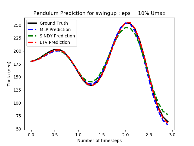
((a))

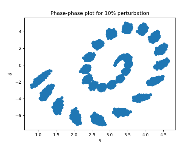
((b))

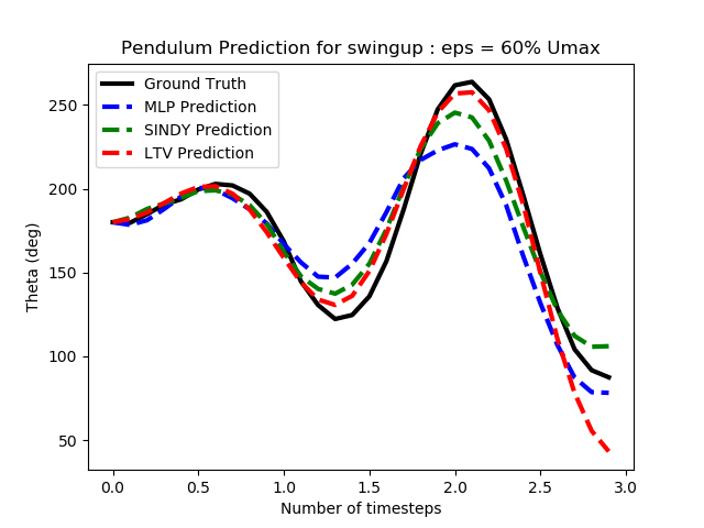
((c))

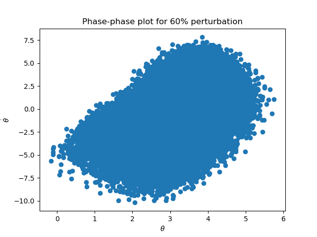
((d))

Figure 2: Comparing the performance of the nonlinear SINDY and MLP models with the LTV model on swing-up pendulum trajectories.

Similar to the pendulum, we generate the optimal trajectory and control for the modified Cartpole swingup task: Starting from the downward position of the pendulum ($\theta_{0}=180^{\circ}$) and the cart at rest, the cart needs to move such that the pendulum comes to rest at $\theta_{T}=60^{\circ}$ within 30 time-steps. The training and testing data size and sampling methods remain the same (Fig. 3). Please note that the random perturbations of the optimal control implicitly defines the sampling distribution in the state space (Fig. 2).

For the Fish robot, we define the optimal control task of moving from the origin to the target co-ordinates $(0.4,0.2,1)$ within 600 time-steps. However, the nonlinear surrogate models exhibit significant deviations from the physical system, making them impractical (Fig. 4). Therefore, we will focus our analysis on the Pendulum and Cartpole systems, which remain practical while still highlighting the identified issues.

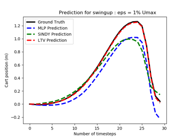
((a))

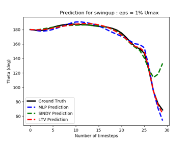
((b))

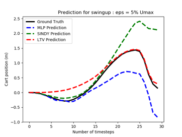
((c))

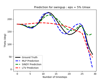
((d))

Figure 3: Comparing the performance of the SINDY and MLP models with the LTV model on swing-up Cartpole trajectories.

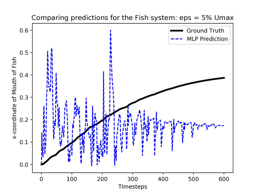
((a))

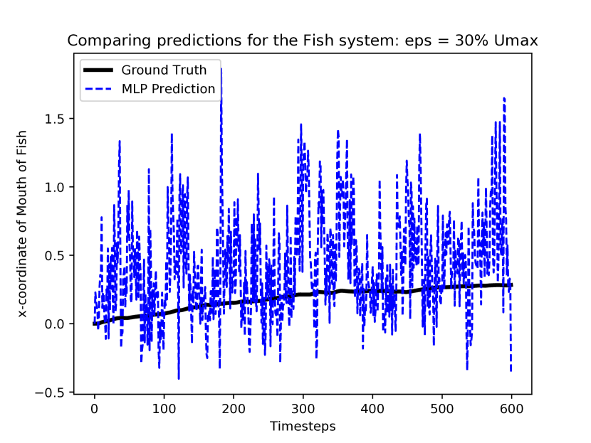
((b))

Figure 4: Performance of the surrogate models on Fish trajectories.

IV-B Model Convergence

For a fixed set of basis functions, the models trained should be invariant to the training data samples, provided that the sampling distribution is the same across the experiments. Thus, for the same sampling distribution, the MLP or SINDy algorithms should converge to the same set of model parameters when re-sampling a different data-set from the same sampling distribution. To verify this experimentally, we sample multiple data-sets from the same sampling distribution by changing the random seed. From the SINDy model, it is easy to test for convergence. With the models trained on the different datasets, we give the optimal control trajectory as our input to all the predictors. From Fig. 5, we observe that the predictions, and correspondingly the learned dynamics, start to diverge as we increase the sampling neighbourhood around the optimal trajectory, showing a lack of convergence as opposed to the low perturbation case. Similarly, for the MLP model, we compare the predictions from the models corresponding do the different datasets (Fig. 6) and observe that the models have very different predictions.

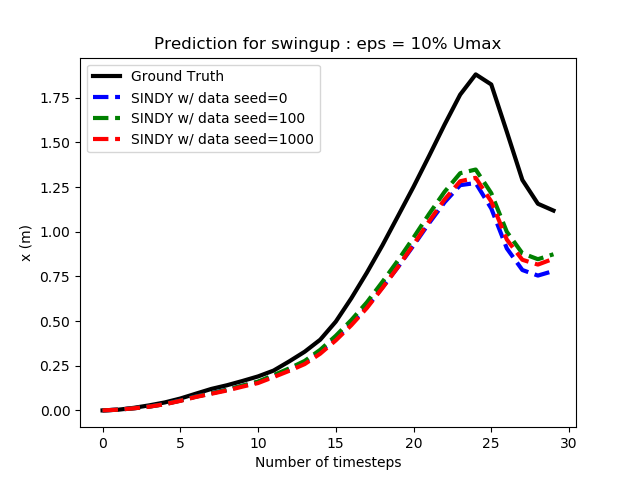
((a))

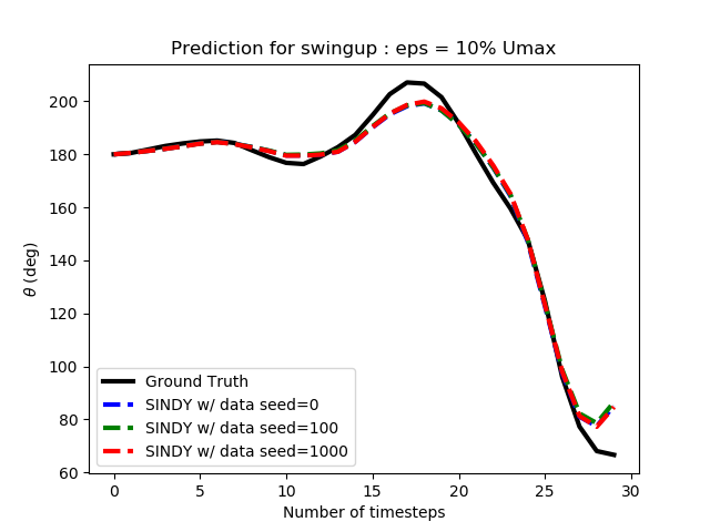
((b))

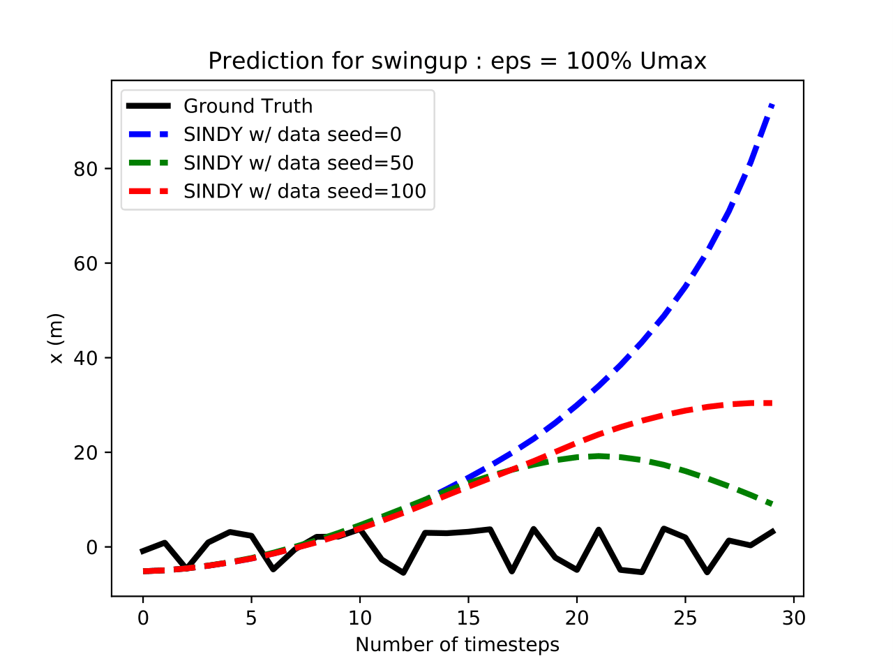
((c))

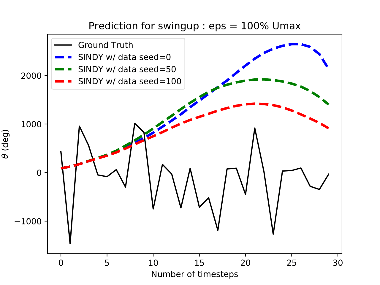
((d))

Figure 5: Convergence of the SINDY model learned on datasets with random initial seeds, with perturbations of $10\%U_{max}$ (a)-(b), and $100\%U_{max}$ (c)-(d) w.r.t. the optimal swingup trajectory.

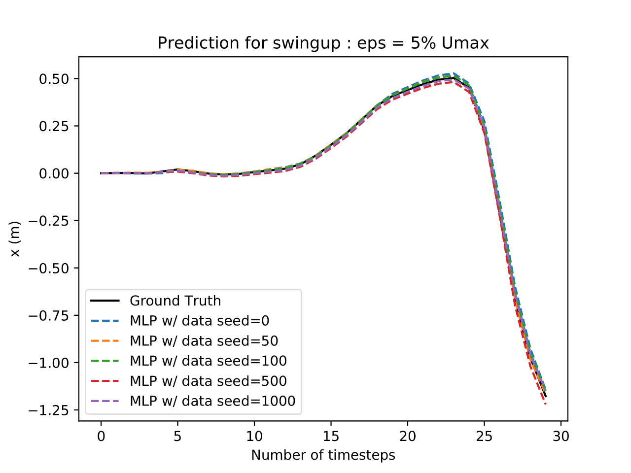
((a))

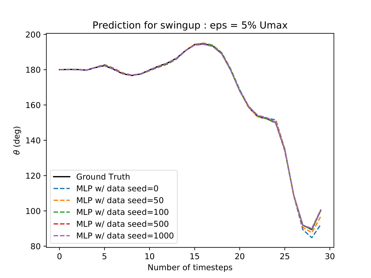
((b))

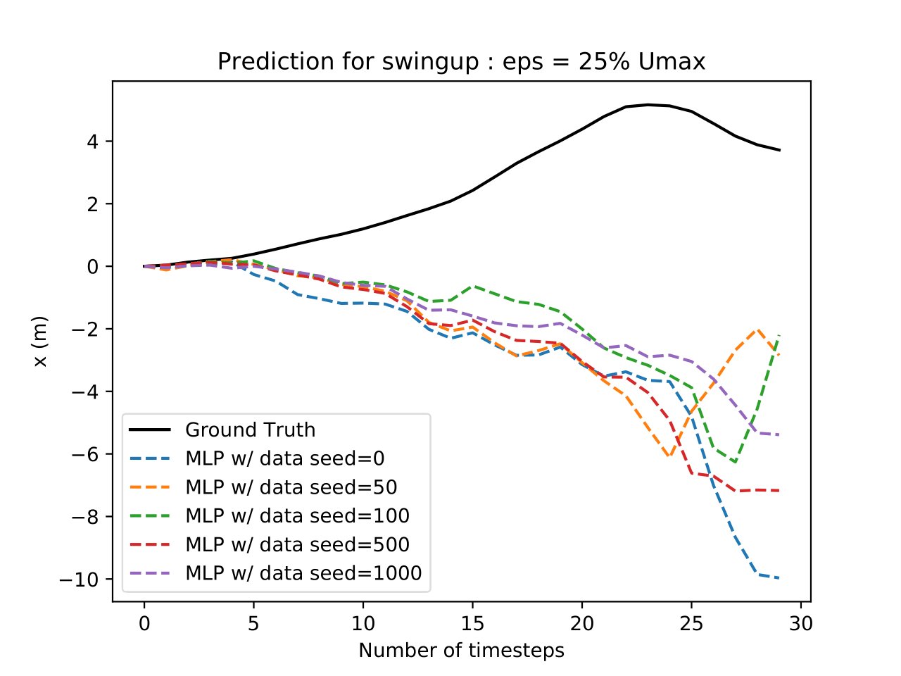
((c))

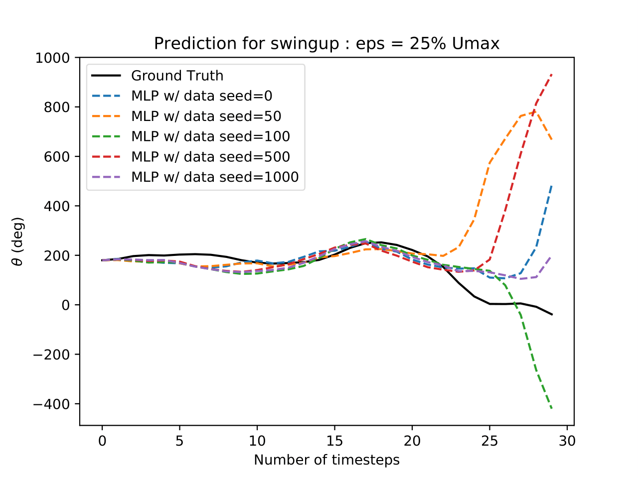
((d))

Figure 6: Convergence of the MLP model learned on datasets with random initial seeds, with perturbations of $5\%$ $U_{max}$ (a)-(b) and $25\%$ $U_{max}$ (c)-(d) w.r.t. the optimal swingup trajectory.

IV-C Ill-Conditioning and Variance

It is straightforward to check for ill-conditioning in the Gram matrix for least-squares based estimators such as SINDy. Given the model, we can compute the Gram-matrix through the data vector $\bar{X}$,i.e., $\mathcal{G}=\{\mathcal{G}_{kl}\}=\frac{1}{R}\bar{X}^{T}\bar{X}$. Then, we can utilize the singular-value decomposition to find the conditioning of the Gram matrix (see Fig. 7).

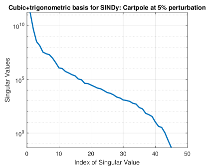
((a))

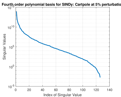
((b))

Figure 7: Conditioning of the SINDY model learned on perturbations of $5\%U_{max}$ w.r.t. the optimal Cartpole swingup trajectory. We assume two sets of basis functions.

For the MLP algorithm, we study the conditioning of the Gram matrix $\frac{1}{R}H_{t}^{R^{\prime}}H_{t}^{R}$ at convergence. It is observed that the matrix is highly ill-conditioned in this case as well (Fig. 8).

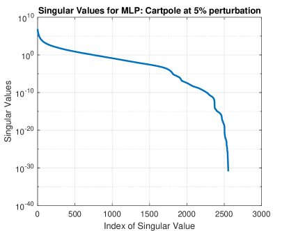
((a))

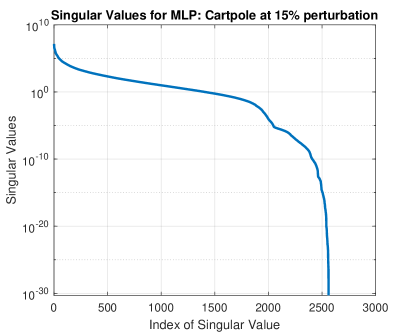
((b))

Figure 8: Observing the conditioning of the MLP model learned on perturbations of (a) $5\%$ and (b) $15\%$ of $U_{max}$ w.r.t. the optimal Cartpole swingup trajectory.

To check for the variance in estimates from SINDy, we train surrogate models on different datasets, and we plot the projections of the error w.r.t. the nonlinear basis (see Fig. 7) clearly showing variance in the estimates. Similarly, we train multiple MLP models on each of the data sets, drawn as before from the same sampling distribution, and observe the vector $\frac{1}{R}H_{t}^{R^{\prime}}\Delta^{R}$ corresponding to each of these models, at different points along the iterations leading up to convergence (Fig. 10). The plots demonstrate variance at different time steps in the training, leading to very different descent directions for different data sets, leading to very different solutions for different datasets.

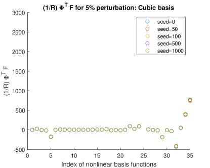
((a))

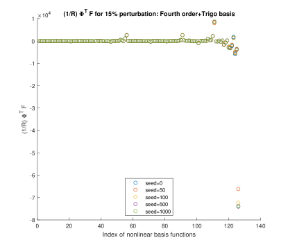
((b))

Figure 9: Variance in the SINDY model, learned on perturbations of $5\%$ and $15\%$ of $U_{max}$ w.r.t. the optimal Cartpole swingup trajectory. It is observed that the variance increases with increase in perturbation, as well as increase in order of the basis functions.

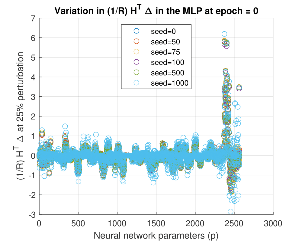
((a))

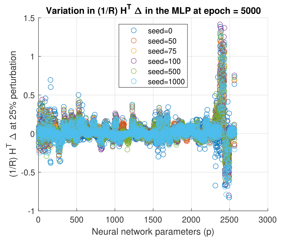
((b))

Figure 10: Variance in the MLP model training, learned on perturbations of $5\%$ of $U_{max}$ w.r.t. the optimal Cartpole swingup trajectory.

IV-D Optimal Control

Given that our problem formulation is rooted in solving the optimal control problem, we can now utilize our trained nonlinear surrogate models to compute the optimal control for our corresponding problems, and benchmark them with the approach using a linear time-varying system identification. In general, we observe that, when using the erroneous models learned by the nonlinear system identification techniques, our control algorithm fails to converge to the optimal solution, despite sampling around the true optimum (Fig. 11 (c)-(d)). This is in stark contrast to the LTV approach, wherein we can start the sampling anywhere in the state space, and still arrive at the true solution by progressively resampling the state space as the algorithm progresses (Fig. 11 (a)-(b)). Thus, adopting a local LTV system identification approach has an insurmountable advantage over the nonlinear data-driven system identification techniques in the context of optimal control.

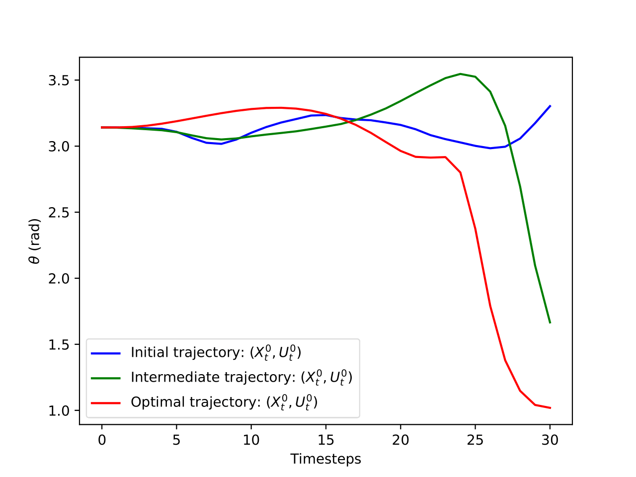
((a))

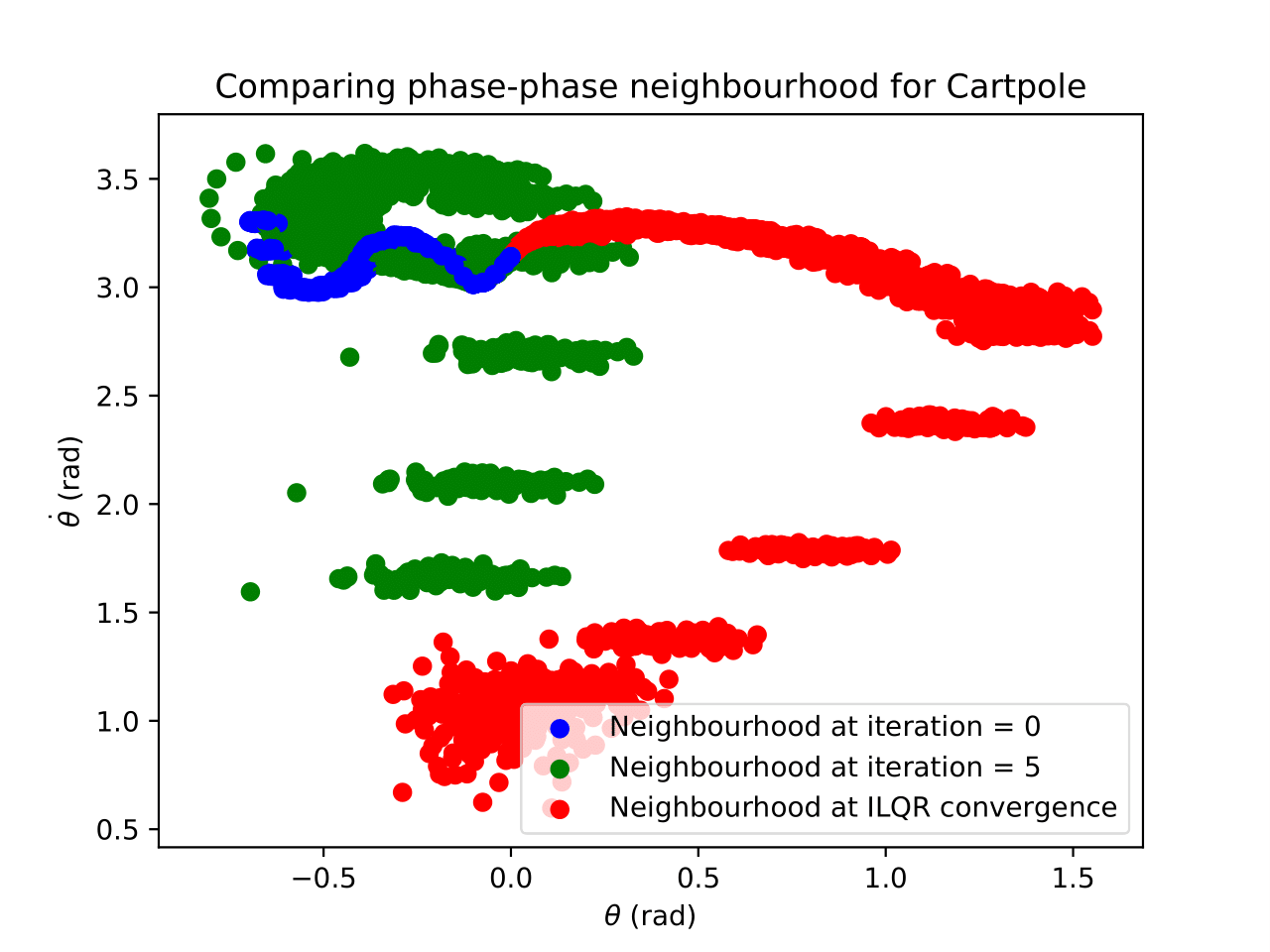
((b))

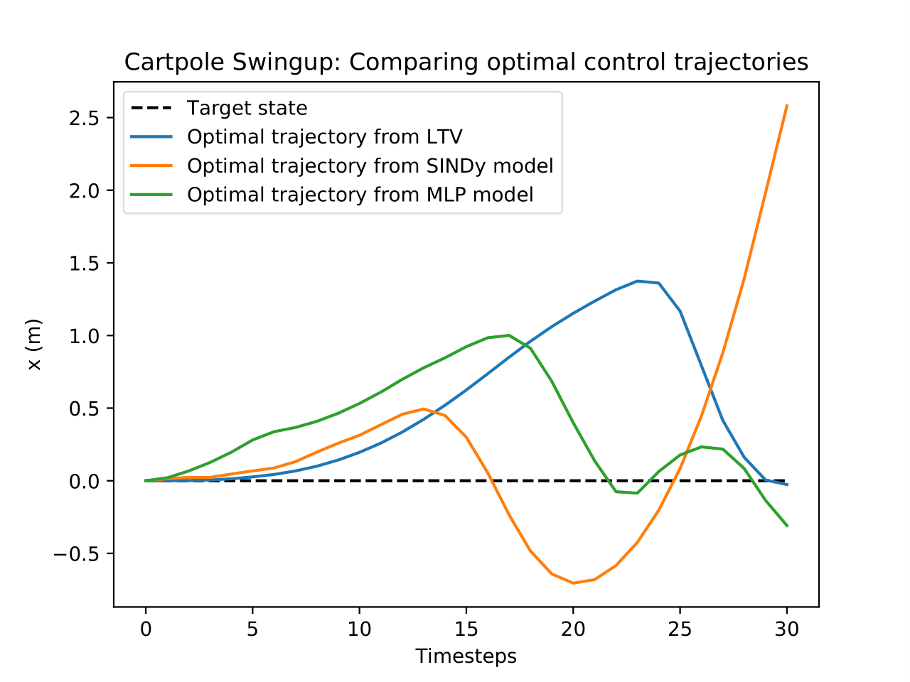
((c))

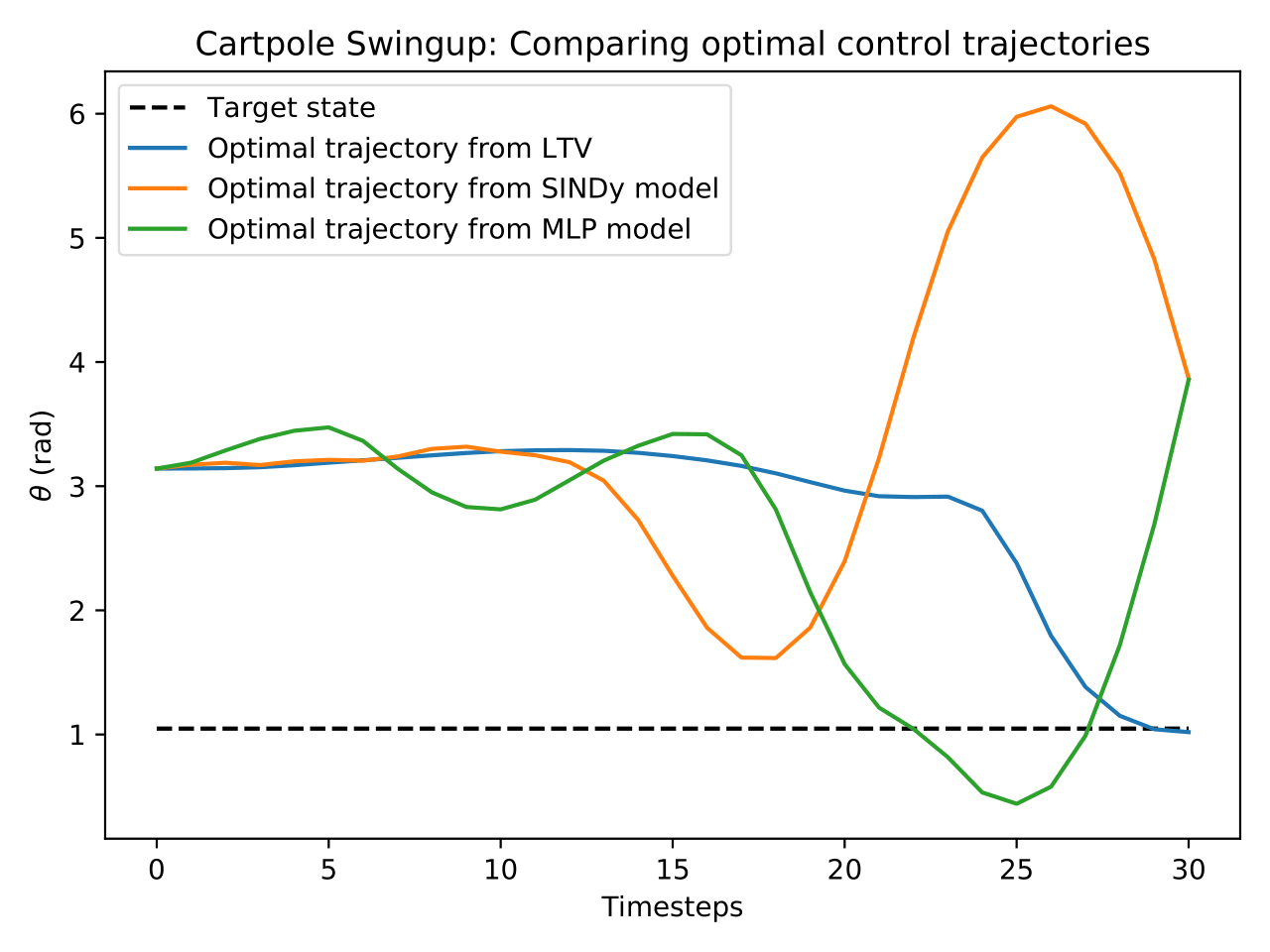
((d))

Figure 11: Optimal control of the Cartpole system when using the LTV model as compared to the MLP and SINDy models where the cartpole system needs to reach the upright position at the origin. The local LTV model can start from a random trajectory and still arrive at the correct solution (a)-(b), while the MLP and SINDy based optimal control, despite aspiring to be ‘global’ models, fail to converge to the optimal (c)-(d).

V Conclusions

In this article, we have shown the equivalence of nonlinear system identification to the problem of generalized moment estimation of a given underlying sampling distribution, bringing to clear focus the inherent problems of ill-conditioning and variance naturally incurred by these methods. The empirical evidence clearly demonstrates the ill-conditioning of the Gram matrix, along with the high variance in the forcing function of the constituent Normal equations. Finally, we have also demonstrated that in the context of optimal nonlinear control, the use of a ‘local’ LTV suffices, and is necessary, to combat the issues inherent to nonlinear surrogate models achieving the global optimum answer. In the future, we plan to extend the analysis and experiments to nonlinear time-varying function approximators, such as RNNs and LSTMs.

References

- [1] S. L. Brunton, J. L. Proctor, and J. N. Kutz, “Discovering governing equations from data by sparse identification of nonlinear dynamical systems,” Proceedings of the national academy of sciences, vol. 113, no. 15, pp. 3932–3937, 2016.
- [2] E. Todorov and W. Li, “A generalized iterative LQG method for locally-optimal feedback control of constrained nonlinear stochastic systems,” in Proceedings of American Control Conference, 2005, pp. 300 – 306.
- [3] F. Giri and E.-W. Bai, Block-oriented nonlinear system identification. Springer, 2010, vol. 1.
- [4] M. Schoukens, A. Marconato, R. Pintelon, G. Vandersteen, and Y. Rolain, “Parametric identification of parallel wiener–hammerstein systems,” Automatica, vol. 51, pp. 111–122, 2015.
- [5] J. Paduart, L. Lauwers, J. Swevers, K. Smolders, J. Schoukens, and R. Pintelon, “Identification of nonlinear systems using polynomial nonlinear state space models,” Automatica, vol. 46, no. 4, pp. 647–656, 2010.
- [6] T. B. Schön, A. Wills, and B. Ninness, “System identification of nonlinear state-space models,” Automatica, vol. 47, no. 1, pp. 39–49, 2011.
- [7] S. A. Billings, Nonlinear system identification: NARMAX methods in the time, frequency, and spatio-temporal domains. John Wiley & Sons, 2013.
- [8] P. Mattsson, D. Zachariah, and P. Stoica, “Recursive identification method for piecewise arx models: A sparse estimation approach,” IEEE Transactions on Signal Processing, vol. 64, no. 19, pp. 5082–5093, 2016.
- [9] K. Narendra, “Identification and control of dynamical systems using neural networks,” IEEE Transactions on Neural Networks, vol. 1, no. 1, pp. 183–192, 1989.
- [10] H. Dinh, S. Bhasin, and W. E. Dixon, “Dynamic neural network-based robust identification and control of a class of nonlinear systems,” in 49th IEEE Conference on Decision and Control (CDC). IEEE, 2010, pp. 5536–5541.
- [11] O. Ogunmolu, X. Gu, S. Jiang, and N. Gans, “Nonlinear systems identification using deep dynamic neural networks,” arXiv preprint arXiv:1610.01439, 2016.
- [12] M. Schoukens and J. P. Noël, “Three benchmarks addressing open challenges in nonlinear system identification,” IFAC-PapersOnLine, vol. 50, no. 1, pp. 446–451, 2017.
- [13] J. Schoukens and L. Ljung, “Nonlinear system identification: A user-oriented road map,” IEEE Control Systems Magazine, vol. 39, no. 6, pp. 28–99, 2019.
- [14] L. Ljung, System Identification: Theory for the User, ser. Prentice Hall information and system sciences series. Prentice Hall PTR, 1999. [Online]. Available: https://books.google.com/books?id=nHFoQgAACAAJ
- [15] R. Pintelon and J. Schoukens, System Identification: A frequency Domain Approach, 2nd ed. Wiley / IEEE Press, Apr. 2012, iEEE Press, Wiley.
- [16] S. Billings, “Nonlinear system identification: Narmax methods in the time, frequency, and spatio-temporal domains,” Nonlinear System Identification: NARMAX Methods in the Time, Frequency, and Spatio-Temporal Domains, 08 2013.
- [17] T. P. Lillicrap, J. J. Hunt, A. Pritzel, N. Heess, T. Erez, Y. Tassa, D. Silver, and D. Wierstra, “Continuous control with deep reinforcement learning,” arXiv preprint arXiv:1509.02971, 2015.
- [18] J. Schulman, S. Levine, P. Abbeel, M. Jordan, and P. Moritz, “Trust region policy optimization,” in International conference on machine learning. PMLR, 2015, pp. 1889–1897.
- [19] J. Schulman, F. Wolski, P. Dhariwal, A. Radford, and O. Klimov, “Proximal policy optimization algorithms,” arXiv preprint arXiv:1707.06347, 2017.
- [20] R. Wang, K. S. Parunandi, A. Sharma, R. Goyal, and S. Chakravorty, “On the search for feedback in reinforcement learning,” in 2021 60th IEEE Conference on Decision and Control (CDC). IEEE, 2021, pp. 1560–1567. [Online]. Available: https://arxiv.org/abs/2002.09478
- [21] D. Yu and S. Chakravorty, “A decoupled data based control (d2c) approach to generalized motion planning problems,” in 2019 IEEE 58th Conference on Decision and Control (CDC). IEEE, 2019, pp. 7281–7286.
- [22] W. Li and E. Todorov, “Iterative linear quadratic regulator design for nonlinear biological movement systems.” in ICINCO (1). Citeseer, 2004, pp. 222–229.