Optimal Symbolic Bound Synthesis

Abstract.

The problem of finding a constant bound on a term given a set of assumptions has wide applications in optimization as well as program analysis. However, in many contexts the objective term may be unbounded. Still, some sort of symbolic bound may be useful. In this paper we introduce the optimal symbolic-bound synthesis problem, and a technique that tackles this problem for non-linear arithmetic with function symbols. This allows us to automatically produce symbolic bounds on complex arithmetic expressions from a set of both equality and inequality assumptions. Our solution employs a novel combination of powerful mathematical objects—Gröbner bases together with polyhedral cones—to represent an infinite set of implied inequalities. We obtain a sound symbolic bound by reducing the objective term by this infinite set.

We implemented our method in a tool, AutoBound, which we tested on problems originating from real Solidity programs. We find that AutoBound yields relevant bounds in each case, matching or nearly-matching upper bounds produced by a human analyst on the same set of programs.

1. Introduction

In this paper we introduce and address the following problem, which we call the optimal symbolic-bound synthesis (OSB) problem:

Given a (potentially non-linear) formula $\phi$ representing assumptions and axioms and an objective term $t$, find a term $t^{*}$ such that

1. (Bound) $\phi\models t\leq t^{*}$

2. (Optimality) For every term $s$ that satisfies the first condition, $t^{*}\preceq s$ holds, where $\preceq$ represents some notion of “term desirability.”

A solution to this problem has many applications in the automatic analysis of programs. For example, a common program-analysis strategy is to extract the semantics of a program as a logical formula, say $\phi$. However, such a formula can contain temporary variables and disjunctions, and is therefore it is difficult for a human to understand the dynamics of the program from $\phi$. An instance of the OSB problem allows a user to specify a term of interest $t$, e.g. representing some resource, such as time, space or the value of some financial asset, and a term order $\preceq$ that strictly favors terms only over input parameters. In this instance an OSB solver produces a sound upper-bound $t^{*}$ on the resource $t$ with all the temporary variables projected out.

The problem of finding constant bounds on a term $t$ given assumptions $\phi$ is commonly addressed in the field of optimization. However, in the context of program analysis we are often not interested in constant bounds on such a term—either because $t$ is unbounded, or because the bound on $t$ is so loose as to be uninformative. An alternative approach—the one adopted in this paper—is to find a symbolic bound, given assumptions $\phi$.

The OSB problem as given above is very general. Namely, we have yet to specify any restrictions on $\phi$, $\models$, or the term-desirability order $\preceq$. In future we would like others to consider methods to address OSB problems for various instantiations of $\models$ and $\preceq$. In this paper, we consider the OSB problem in the context in which $\phi$, $\models$ and $t$ are interpreted over non-linear arithmetic, and $\preceq$ gives a intuitive, human notion of a simpler term. Moreover, we do not place a restriction on the form of $\phi$. That is, $\phi$ is an arithmetic formula with the usual boolean connectives.

This setting introduces the significant challenge of non-linear arithmetic reasoning: (i) in the case of rational arithmetic, it is undecidable to determine whether any $t^{\prime}$ is a bound on $t$, let alone find an optimal bound; (ii) in the case of real arithmetic, reasoning is often prohibitively expensive. In the setting of finding bounds, the challenge is finding a finite object to represent the infinite set of upper-bounds implied by the formula $\phi$. In the case of linear arithmetic, convex polyhedra can be represented finitely, and can completely represent the set of inequality consequences of a linear formula $\phi$. Moreover, manipulating polyhedra is often reasonably efficient. However, in the non-linear rational case no such complete object exists, and in the non-linear real case manipulating the corresponding object is computationally challenging.

To address this challenge we introduce a mathematical object we call a cone of polynomials (§4.3) to hold on to an infinite set of non-linear inequalities. A cone of polynomials, consists of a polynomial ideal (§3.1), which captures equations, and a polyhedral cone (§3.2), which captures inequalities. Cones of polynomials strike a balance between expressiveness and computational feasibility—using non-linear reasoning on equalities through the ideal, and linear reasoning on inequalities through the linear cone, gives efficient yet powerful non-linear reasoning on inequalities.

We utilize cones of polynomials to address the non-linear OSB problem in a two-step process: (1) From $\phi$ create an implied cone of polynomials $C$. That is, $C$ is an infinite collection of inequalities, each implied by $\phi$. (2) Reduce the term $t$ by $C$ to obtain $t^{*}$.

Due to the difficulties of non-linear arithmetic the first step is necessarily incomplete. However, the second step (reduction) is complete with respect to cones of polynomials. Our reduction method for cones of polynomials makes use of a sub-algorithm that reduces a linear term by a polyhedron. That is, in §4.2 we give an algorithm (Alg. 2) that solves the OSB problem, where $\phi$ is a conjunction of linear inequalities (a polyhedron), $\models$ is interpreted as linear arithmetic, and $\preceq$ is an order that encodes preferability of the dimensions of the returned bound. This method makes use of a novel local projection (§4.2) method. Local projection can be seen as an incomplete method of quantifier elimination for polyhedra that avoids the blow-up of a full-projection method such as Fourier-Motzkin. Nevertheless, local projection suffices in the case of the OSB problem for polyhedra. In §7, we compare our reduction method based on local project with a, perhaps more obvious, approach based on multi-objective linear programming. We find that our algorithm solves the problem much more efficiently than the LP approach.

In §4.3, we show (Thm. 4.3.1) how the polyheral OSB solution can be extended to the setting of cones of polynomials. This means that in particular we are able to completely solve OSB with respect to a polynomial $t$ and a polynomial cone $C$, which has the property that the result, $t^{*}$, is optimal with respect to any other bound $s$ implied by the cone $C$. This method works for desirability orders $\preceq$ that are monomials orders.

With these methods in hand, §5 shifts to the following problem: Given a formula $\phi$, extract an implied cone $C$ for which the methods from §4 can be applied. Due to the issues of non-linear arithmetic, such an extraction process will necessarily be incomplete. However, in §5 we give a heuristic method for extracting a cone from a non-linear formula that works well in practice (§7). Moreover, our method allows $\phi$ and $t$ to contain function symbols, such as $\left\lfloor\cdot\right\rfloor$ and $\frac{1}{\cdot}$ (reciprocal), both of which are outside the signature of polynomial arithmetic. Overall, our two-step method is sound with respect to non-linear arithmetic augmented with additional function symbols.

In §6, we introduce the effective-degree order. Effective-degree is essentially a degree monomial orders, extended to the case of non-polynomial function symbols. Effective-degree orders capture the intuitive notion that terms with fewer products are simpler. Also, variable restriction can be encoded as an effective-degree order.

Our saturation and reduction methods combined with effective degree results in a powerful yet practical method for addressing the non-linear OSB problem. In §7, we give experimental results that show our method, using effective-degree as a term desirability order, produces interesting and relevant bounds using a set of benchmarks extracted from Solidity code by industry experts in smart-contract verification. Our tool is able to produce in seconds or minutes bounds which match or nearly-match human-produced bounds, as well as bounds where ones were previously unknown to human experts.

Contributions

1. The introduction of the optimal symbolic-bound synthesis problem

2. The local-projection method for projecting polyhedra (§4.1)

3. Algorithms for reducing a term $t$ by a polyhedron (§4.2) and a polynomial cone (§4.3)

4. A saturation method that extracts a polynomial cone from a non-linear formula with additional function symbols (§5)

5. The introduction of the effective-degree order on terms, which is amenable to automation, and in practice results in useful bounds (§6)

6. An experimental evaluation demonstrating the power and practicality of our method (§7)

§9 discusses related work. Proofs of theorems are given in appendices.

2. Overview

⬇

class Rebase {

uint base

uint elastic

function add(amount) {

a2base = toBase(amount)

elastic += amount

base += a2base

}

function toBase(x) {

x * this.base / this.elastic

}

}

(a) Extracted Solidity code.

(b) Overview of the method

To motivate the optimal symbolic-bound synthesis problem, as well as understand how we address it, consider the code in Fig. 1(a). This code presents us with an interesting non-linear inequational-reasoning problem, which arises from a common smart-contract pattern. A typical “rebase” or “elastic” smart contract holds some amount of “tokens,” which can vary over time, and each user holds a certain amount of “shares” in the tokens. While the number of tokens may vary (e.g., to control the price), the given number of shares that the user holds should correspond to a largely-unchanging percentage of the total tokens. The utility class Rebase, which is based on real-world Solidity code, tracks the total number of tokens in elastic and the total number of shares in base. The function add increases the number of tokens, and the number of available shares accordingly. However, a given amount $v$ should be represented by the same number of shares even after an add operation. Thus, for a given values $v$ and $a$, if we execute the sequence

x = toBase(v); add(a); y = toBase(v),

the term $t=x-y$ should be $0$, or close to $0$. Plugging in concrete value shows that $t$ is not identically $0$, but how far from $0$ is it? The answer can depend on $v$ and $a$, as well as the initial values of elastic, and base, so a precise characterization involves a symbolic expression. Indeed, a verification expert that analyzed this problem came up with the bound $t\leq 1+\left\lfloor v/(e+a)\right\rfloor$, where $e$ is the initial value of elastic. Can we automate this creative process of generating a bound, which for humans often involves much trial-and-error, while even validating a guess for a bound is challenging? In this case, can we automatically find lower and upper symbolic bounds on the term t = x-y?

The same question can be translated to an OSB problem by writing the following conjunctive formula that represents the assumptions about the initial state, together with the program’s execution:

$$\phi\triangleq x=\left\lfloor\frac{vb}{e}\right\rfloor\land y=\left\lfloor\frac{vb^{\prime}}{e^{\prime}}\right\rfloor\land a2=\left\lfloor\frac{ab}{e}\right\rfloor\land e^{\prime}=e+a\land b^{\prime}=b+a2\land a,b,e,v\geq 0.$$

The goal is to produce a term $t^{*}$ such that $\phi\models x-y\leq t^{*}$. Furthermore, we are interested in terms that are “insightful” in some sense. For example, we would like to produce a bound that does not contain any temporary variables $e^{\prime}$, $a2$, or $b^{\prime}$, as well as the variables $x$ and $y$. This variable restriction does not alone determine a desirable bound, but for this example we at least require a bound to satisfy this constraint. For this example, as well as our experiments, we use the effective-degree order (§6) as a stand-in for term desirability. Using effective-degree we can encode variable restriction into the order, ensuring that the variables $e^{\prime}$, $a2$, $b^{\prime}$, $x$, and $y$ are absent from the bound we produce if such a bound exists. Effective-degree goes further and roughly minimizes the number of products in the result.

Fig. 1(b) gives an outline of our method. The first step to produce an implied cone is to purify the formula $\phi$ into a formula using only polynomial symbols. We do this by introducing a new variable for each non-polynomial function, and placing the variable assignment in a foreign-function map. That is, for every non-polynomial function symbol $f(w)$ we introduce a new variable, $u$, add $u\mapsto f(w)$ to our map and replace $f(w)$ with $u$. Purifying the formula $\phi$ we obtain,

$$\phi^{\prime}\triangleq\ x=u_{4}\land y=u_{5}\land a2=u_{6}\land e^{\prime}=e+a\land b^{\prime}=b+a2\land a,b,e,v\geq 0$$

$$TM= \{u_{1}\mapsto e^{-1},u_{2}\mapsto e^{\prime-1},u_{3}\mapsto e^{-1},u_{4}\mapsto\left\lfloor vbu_{1}\right\rfloor,u_{5}\mapsto\left\lfloor vb^{\prime}u_{2}\right\rfloor,u_{6}\mapsto\left\lfloor abu_{3}\right\rfloor\}$$

The purpose of purification is to produce a $\phi^{\prime}$ which contains no function symbols. The original formula $\phi$ is equivalent to $\phi^{\prime}\land\bigwedge_{u\mapsto f(w)}u=f(w)$. By making this separation of $\phi$ in $\phi^{\prime}$ and $TM$ we can create methods that can separately work on $\phi^{\prime}$, $TM$, or the combination of $\phi^{\prime}$ and $TM$ when required. We then strengthen $\phi^{\prime}$ by adding properties of the functions in $TM$. This is the Instantiate Axioms step in Fig. 1(b). For example, $u_{4}$ represents a floor term and so satisfies more properties than a generic polynomial variable. Thus, after purification our method uses the term map $TM$ to instantiate axioms for floor and inverse for each occurrence of a floor and inverse term appearing in the map, and adds them to $\phi^{\prime}$. That is, we create $\phi^{\prime\prime}$ by adding the instantiated axioms $(u_{1}e=1)$, $(u_{2}e^{\prime}=1)$, …, $vbu_{1}-1\leq u_{4}\leq vbu_{1}$, $vb^{\prime}u_{3}-1\leq u_{5}\leq vb^{\prime}u_{3}$, …, $e\geq 0\implies u_{1}\geq 0$, $vbu_{1}\geq 0\implies u_{4}\geq 0$, etc, to $\phi^{\prime}$. At this point $\phi^{\prime\prime}$ is

$$\phi^{\prime\prime}\triangleq\ \phi^{\prime}\land (e\geq 0\implies u_{1}\geq 0)\land\dots\land(eu_{1}=1)\land\dots\land(vbu_{1}-u_{4}\geq 0)\land\dots$$

After axioms have been instantiated, $\phi^{\prime\prime}$ and the term map $TM$ are used to construct a cone of polynomials (§4.3). A cone of polynomials is a composite of a polynomial ideal (§3.1) and a polyhedral cone (§3.2). The ideal and polyhedral cone are each represented by a finite set of basis equations and inequalities, respectively. The ideal consists of its basis equations, as well as all other equations that are polynomially implied by the basis equations. That is, the ideal consists of polynomials $p_{1},\dots,p_{k}$, representing assumptions $p_{i}=0$, as well as any polynomial of the form $h_{1}p_{1}+\dots+h_{k}p_{k}$ for polynomials $h_{1},\dots,h_{k}$. The polyhedral cone consists of its basis inequalities as well as all other inequalities that are linearly implied by the basis inequalities. That is, the polyhedron consists of polynomials $q_{1},\dots,q_{r}$, representing assumptions $q_{i}\geq 0$, as well as any other polynomial of the form $\lambda_{1}q_{1}+\dots\lambda_{r}q_{r}$ for scalar $\lambda_{i}\geq 0$. Overall, the cone consists of terms of the form $p+q$ where $p$ is a member of the ideal and $q$ is a member of the polyhedron. Because $p$ is an implied equation and $q$ is an implied inequality, we have $p+q\geq 0$.

We call the process of creating a cone of polynomials from $\phi^{\prime\prime}$ and $TM$ saturation. We describe the saturation process in §5 using the running example from this section. At a high level, saturation is an iterative process that extracts equalities and inequalities that are implied by $\phi^{\prime\prime}$ and $TM$. A cone of polynomials is created by adding extracted equalities to the ideal part and by adding extracted inequalities to the polyhedral cone part. The methods that we use include congruence closure (§5.1), linear consequence finding (§5.2), and “taking products” (§5.3). By taking products, we mean that from an inequality $w\geq 0$ and $z\geq 0$, we can derive $w^{2}\geq 0$, $wz\geq 0$, $z^{2}\geq 0$, etc. There are an infinite set of products we could add so our method takes products up to a given saturation depth. In our experiments a saturation depth of 3 worked well. By bounding the set of products we add as well as the use of our consequence finding method makes saturation incomplete for full non-linear arithmetic. However, our experiments show saturation works well in practice (§7).

As detailed in §5, saturation produces the following cone of polynomials on the running example:

$$C\triangleq\ \langle x-u_{4},y-u_{5},a2-u_{6},e^{\prime}-e-a,b^{\prime}-b-a2,u_{3}-u_{1},eu_{1}-1,(e+a)u_{2}-1\rangle+$$

$$[e,a,v,b,e^{2},ea,\dots,vbu_{1}-u_{4},vu_{2}u_{6},vbu_{2}-vbu_{1}+vu_{2},u_{5}-vu_{2}u_{6}-vbu_{2}+1,1];$$

$\langle x-u_{4},\dots,\rangle$ is the ideal and $[e,\dots,1]$ is the polyhedral cone. In other words, saturation extracted the equations $x-u_{4}=0$, $y-u_{5}=0$, etc. as well as the inequalities $e\geq 0$, $a\geq 0$, and many more.

The next step in addressing the OSB problem is to reduce our term of interest by $C$. That is, we need to find the best $t^{*}$ such that the cone implies $t\leq t^{*}$. Equivalently, the problem is to find the best $t^{*}$ such that the cone contains $t^{*}-t$. Our reduction procedure for polynomials and polynomial cones works by first reducing the polynomial of interest by the ideal, and then reducing the result by the polyhedron. The process of reducing the polynomial by the ideal is a standard method in computational algebraic geometry (§3.1); however, we present a novel polyhedral reduction method (§4.2), which in turn uses a novel projection method (§4.1).

The main idea of our polyhedral reduction method is to order the dimensions of the polyhedron, which in our setting correspond to monomials, and successively project out the worst dimension of the polyhedron until the term of interest $t$ becomes unbounded. We show (Thm. 4.2) that the bound on $t$ right before $t$ becomes unbounded is optimal in the order of dimensions. In §4.3, we show that the combination of the standard ideal reduction with the polyhedral reduction yields a reduction method for the combined cone.

For the example from Fig. 1(a), we instantiate an effective-degree order that favors terms without temporary variables. From the saturated cone of polynomials $C$, we have the following equations in the basis of the ideal, $x-u_{4}$ and $y-u_{5}$, as well as the following inequalities in the basis of the polyhedral cone:

$$vbu_{1}-u_{4}\geq 0\qquad va2u_{2}+vbu_{2}-vbu_{1}+vu_{2}\geq 0\qquad u_{5}-va2u_{2}-vbu_{2}+1\geq 0$$

Reducing $x-y$ by the equations yields $u_{4}-u_{5}$. The polyhedral reduction method can then be seen as rewriting $u_{4}-u_{5}$ to $vu_{2}+1$ via the justification

$$vu_{2}+1-(u_{4}-u_{5})=vbu_{1}-u_{4}+va2u_{2}+vbu_{2}-vbu_{1}+vu_{2}+u_{5}-va2u_{2}-vbu_{2}+1$$

The right-hand-side is non-negative. Thus, $x-y\leq vu_{2}+1$. Before returning the final result, our system unpurifies this bound by replacing $u_{2}$ with its definition in $TM$. Consequently, our system returns the final result as “$x-y\leq\frac{v}{a+e}+1$.” Our system can also be used to automatically find a lower bound for a term. In our example, the lower bound that it finds is “$x-y\geq-1$.”

These bounds, $-1\leq x-y\leq\frac{v}{a+e}+1$, which the implementation of our method found on the order of seconds, are very nearly the bounds, $0\leq x-y\leq\left\lfloor\frac{v}{a+e}\right\rfloor+1$, found manually by a human analyst. Differences between the bound we compute automatically and the bound produced by a human sometimes stem from slightly different preferences in the tension between the bound’s simplicity and tightness, but in this case a deeper issue is at play. Our method has a limited capacity to perform inequality reasoning inside a floor term; for instance, we do not produce the inequality $\left\lfloor t_{1}\right\rfloor\leq\left\lfloor t_{2}\right\rfloor$ even when $t_{1}\leq t_{2}$ is known, if $t_{1}$ or $t_{2}$ are not present in the input formula. We do obtain the slightly weaker $\left\lfloor t_{1}\right\rfloor\leq t_{2}$, which, for instance, does not precisely cancel with $-\left\lfloor t_{2}\right\rfloor$, leading to slightly weaker bounds.

Our initial experience with the system is that it is able to produce interesting upper bounds that are challenging to come up with manually. In one case (fixed point integer arithmetic—see §7), we asked a human analyst to propose a bound for a problem they knew, but had previously attempted only a bound in the other direction (whereas our system computes both at the same time). After approximately fifteen minutes, and correcting the derivation at least once, they came up with a bound that nearly matches the bound that our system generated in less than a second.

3. Background

Our method is based on the construction and manipulation of a cone, which as stated consists of a polynomial ideal to hold on to equations and a linear cone to hold on to inequalities. Part of our contribution is the use and manipulation of this composite object. However, we borrow many techniques and ideas from the study of the individual components. In this section, we give background on the definitions and properties of polynomials ideals and linear cones.

Overall, our method works for any ordered field. That is, our techniques are sound with respect to the theory of ordered fields. We will write $\models_{\textit{OF}}$ to denote entailment modulo the theory of ordered fields when we want to indicate soundness. Since $\mathbb{R}$ and $\mathbb{Q}$ are ordered fields, $\models_{OF}$ implies entailment with respect to non-linear real and non-linear rational arithmetic.

3.1. Polynomials and Ideals

In this section, we give definitions of polynomial ideals, as well as highlight algorithms and results that we will need in order to manipulate and reason about polynomial ideals. For a more in-depth presentation of polynomial ideals and algorithms for manipulating them, see Cox et al. (2015).

Our use of the phrase monomial refers to the standard definition. We consider polynomials as being a finite linear combination of monomials over some (ordered) field $\mathbb{K}$. For example $\mathbb{K}$ could be $\mathbb{Q}$ or $\mathbb{R}$.

In this paper we use polynomial ideals to represent an infinite set of equality consequences. Due to some classical results from ring theory as well as a result due to Hilbert concerning polynomial ideals, we can take the following definition as a definition for any ideal of polynomials.

Definition 3.1.

Let $\{p_{1},\dots,p_{k}\}$ be a finite set of polynomials. $\langle p_{1},\dots,p_{k}\rangle$ denotes the ideal generated by the basis $\{p_{1},\dots,p_{k}\}$. Furthermore,

$$\langle p_{1},\dots,p_{k}\rangle=\{h_{1}p_{1}+\dots+h_{k}p_{k}\mid 1\leq i\leq k\text{ and }h_{i}\text{ is an arbitrary polynomial}\}.$$

If we consider a set of polynomials $p_{1},\dots,p_{n}$ as a given set of polynomial equations, i.e., $p_{i}=0$ for each $i$, then the ideal generated by $p_{1},\dots,p_{n}$ consists of equational consequences.

Example 3.2.

One way to see that $x-1-t=0\land y-1-t^{2}=0$ $\models_{\textit{OF}}x^{2}-2x=y-2$, is by observing

$$x^{2}-2x-y+2 \in\langle x-1-t,y-1-t^{2}\rangle$$

$$x^{2}-2x-y+2 =(x-1+t)(x-1-t)+(-1)(y-1-t^{2})$$

As will be highlighted shortly, determining ideal membership for $\mathbb{Q}[x_{1},\dots,x_{n}]$, $\mathbb{R}[x_{1},\dots,x_{n}]$ is decidable. However, in the general context of non-linear rational arithmetic or nonlinear integer arithmetic, determining polynomial consequences is undecidable. Therefore, in general ideals give a sound but incomplete characterization of equational consequences. A simple example illustrating this fact is $x^{2}=0\models_{\text{OF}}x=0$, but $x\not\in\langle x^{2}\rangle$.

While polynomial ideals are in general incomplete, they have the advantage of having useful algorithms for manipulation and reasoning. Namely, the multivariate-polynomial division algorithm and the use of Gröbner bases give a practical method to reduce a polynomial by an ideal and check ideal membership. These techniques are integral to our overall method, so we now briefly highlight some of these ideas.

Algorithms for manipulating polynomials often consider the monomials one at a time. Thus, we often orient polynomials using a monomial order.

Definition 3.3.

Let $\ll$ be a relation on monomials. $\ll$ is a monomial order, if

1. $\ll$ is a total order.

2. For any monomials $a$, $b$, and $m$, if $a\ll b$, then $a\cdot m\ll b\cdot m$

3. For any monomial $a$, $a\gg 1$.

With a monomial order defined, we often write polynomials as a sum of their monomials in decreasing order. A strategy for ensuring termination of algorithms is to process monomials in decreasing order with respect to some monomial order, while guaranteeing intermediate steps do not introduce larger monomials. Because a monomial order is well-ordered, termination is ensured.

Common monomial orders are the lexicographic monomial order, degree lexicographic order, and degree reverse lexicographic order (grevlex). The details of these monomial orders in unimportant for this work, but in practice the grevlex order tends to yield the best performance in implementations.

Definition 3.4.

With respect to a monomial order the leading monomial of a polynomial $p$, denoted $\mathrm{LM}(p)$, is the greatest monomial of $p$.

Once a monomial order has been defined, we can use the multivariate polynomial division algorithm to divide a polynomial $f$ by an ideal $\langle p_{1},\dots,p_{k}\rangle$. This algorithm successively divides the terms of $f$ by the leading terms of the set of $p_{i}$’s until no more divisions can be performed. The result is a remainder $r$. The value of this remainder can be used for various purposes. For example, if $r=0$, then $f\in\langle p_{1},\dots,p_{k}\rangle$. However, examples can be constructed that show that performing multivariate division on an arbitrary basis does not necessarily yield a unique result. In other words, it is possible to have another basis $p^{\prime}_{1},\dots,p^{\prime}_{k}$ with $\langle p^{\prime}_{1},\dots,p^{\prime}_{k}\rangle=\langle p_{1},\dots,p_{k}\rangle$, but dividing $f$ by $p^{\prime}_{1},\dots,p^{\prime}_{k}$ will yield a different remainder $r^{\prime}$. The solution to this issue is to divide by a Gröbner basis. That is, to divide a polynomial $f$ by an ideal $\langle p_{1},\dots,p_{k}\rangle$, we do not divide $f$ by $p_{1},\dots,p_{k}$, but instead we construct a Gröbner basis $g_{1},\dots,g_{s}$ with $\langle g_{1},\dots,g_{s}\rangle=\langle p_{1},\dots,p_{k}\rangle$. It can then be shown that dividing $f$ by $g_{1},\dots,g_{s}$ will yield a unique remainder.

The exact definition of a Gröbner basis is technical and not required for this paper. What is required to know is that, given an ideal $\langle p_{1},\dots,p_{k}\rangle$, there are algorithms, such as Buchberger’s algorithm (buchbergerA; buchbergerB) and the F4 (FaugereF4) and F5 (FaugereF5) algorithms, for constructing a Gröbner basis $g_{1},\dots,g_{s}$ with $\langle g_{1},\dots,g_{s}\rangle=\langle p_{1},\dots,p_{k}\rangle$. Furthermore, using the multivariate division algorithm to divide a polynomial $f$ by a Gröbner basis yields a remainder with certain special properties.

Definition 3.5.

Let $B$ be a Gröbner basis, and $f$ a polynomial. We call the process of dividing $f$ by $B$ using the multivariate division algorithm and taking the remainder reduction, and denote the process by $\textbf{red}_{B}(f)$.

Theorem 3.6.

(CLO:2015, Section 2.6) Let $B=\{g_{1},\dots,g_{s}\}$ be a Gröbner basis for an ideal $I$, $f$ a polynomial, and $r=\textbf{red}_{B}(f)$. $r$ is the unique polynomial with the following properties:

1. No term of $r$ is divisible by any of $\mathrm{LT}(g_{1}),\dots,\mathrm{LT}(g_{s})$.

2. There is a $g\in I$ with $f=g+r$.

Lemma 3.7.

$\mathrm{LT}(f)\gg\mathrm{LT}(\textbf{red}_{B}(f))$ for any $f$ and basis $B$.

Let $B=\{g_{1},\dots,g_{s}\}$ be a Gröbner basis for an ideal $I$, $f$ a polynomial, and $r=\textbf{red}_{B}(f)$. $r$ is the optimal remainder in the monomial order. That is, for any other $r^{\prime}$ with $f=g^{\prime}+r^{\prime}$ for some $g^{\prime}\in I$, $\mathrm{LT}(r^{\prime})\gg\mathrm{LT}(r)$. Let $r^{\prime}$ be some polynomial with $f=g^{\prime}+r^{\prime}$. Reducing $r^{\prime}$ by $B$ yields $r^{\prime\prime}$ with $r^{\prime}=g^{\prime\prime}+r^{\prime\prime}$ for some $g^{\prime\prime}\in I$, as well as $\mathrm{LT}(r^{\prime})\gg\mathrm{LT}(r^{\prime\prime})$. Moreover, $r^{\prime\prime}$ satisfies the properties in Thm. 3.6 with respect to $r^{\prime}$. However, $f=g^{\prime}+g^{\prime\prime}+r^{\prime\prime}$, and because $g^{\prime},g^{\prime\prime}\in I$ so is $g^{\prime}+g^{\prime\prime}\in I$. Thus, $r^{\prime\prime}$ also satisfies the conditions of Thm. 3.6 with respect to $f$. Thus, $r=r^{\prime\prime}$ and $\mathrm{LT}(r^{\prime})\gg\mathrm{LT}(r^{\prime\prime})=\mathrm{LT}(r)$.

Corollary 3.8.

Let $B=\{g_{1},\dots,g_{s}\}$ be a Gröbner basis for an ideal $I$, $f$ a polynomial. $f\in I$ if and only if $0=\textbf{red}_{B}(f)$.

3.2. Polyhedral Cones

In this section, we give background on polyhedral cones. Mirroring the process of using ideals to represent equations, we use polyhedral cones to represent inequalities. The reader should keep in mind that our method uses two different kinds of cones. We have an inner cone which is used to hold on to linear inequalities and an outer cone which consists of an ideal and the inner cone. The inner cone is a polyhedral cone and is the main subject on this section. We will describe the outer cone in more detail in §4.3. To make the distinction between the two concepts clear, we will use the terms “polyhedral cone” and “cone of polynomials” to refer to the inner and outer cone, respectively.

Definition 3.9.

Let $\mathbb{K}$ be an ordered field (e.g., $\mathbb{R}$ or $\mathbb{Q}$) and $V$ be a vector space over $\mathbb{K}$. A polyhedral cone $C$ is the conic combination of finitely many vectors. That is, there is a set of vectors $\{v_{1},\dots,v_{n}\}$ with $C=\{\lambda_{1}v_{1}+\dots+\lambda_{n}v_{n}\mid\lambda_{i}\geq 0\}$. We use $C=[v_{1},\dots,v_{n}]$ to denote that $C$ is generated by the vectors $\{v_{1},\dots,v_{n}\}$.

While we use polyhedral cones to represent a set of linear consequences, we frame some of our reduction algorithms (§4.2) in terms of convex polyhedra. Fortunately, there is a very strong connection between polyhedral cones and convex polyhedra. There are multiple equivalent definitions for a convex polyhedron that lead to different representations. In this paper we only represent a polyhedron using a set of inequality constraints, sometimes called the constraint representation.

Definition 3.10.

Let $\mathbb{K}$ be an ordered field. A linear constraint over variables $x_{1},\dots,x_{n}$ is of the form $a_{1}x_{1}+\dots+a_{n}x_{n}+b\geq 0$, $a_{1}x_{1}+\dots+a_{n}x_{n}+b>0$, or $a_{1}x_{1}+\dots+a_{n}x_{n}+b=0$, where $a_{1},\dots,a_{n},b\in\mathbb{K}$. A (convex) polyhedron is the set of points of $\mathbb{K}^{n}$ satisfying a set of linear constraints.

Because each equality can be represented as two inequalities, we could consider polyhedra to not have equality constraints. However, having explicit equalities can allow algorithms to be more efficient in their calculations. We do not take a strong stance on whether all of the equalities of a polyhedron are explicit or not. In §4, we sometimes consider equality constraints as being explicitly part of a polyhedron, but our methods work the same if the equalities are implicit.

If we look at the constraints of the polyhedron as given inequality assumptions, taking conical combinations of the constraints give a sound set of inequality consequences. Moreover, Farkas’ Lemma shows that this set of consequences is also complete.

Lemma 3.11.

(Variant of Farkas’ Lemma) Let $P$ be a non-empty polyhedron with non-strict constraints $N=\{c_{1}\geq 0,\dots,c_{k}\geq 0\}$ and strict constraints $S=\{s_{1}>0,\dots,s_{l}>0\}$. Let $P^{*}$ denote the polyhedral cone $[c_{1},\dots,c_{k},s_{1},\dots,s_{l},\mathbf{1}]$. Then $P\models_{\textit{LRA}}t\geq 0$ if and only if $t\in P^{*}$.

We close this section by giving observing that a polyhedral cone that represents inequalities can also represent equalities in the sense that for some vector $v\in C$ it is possible for $-v\in C$ to hold as well. If $C$ is holding onto non-negative vectors, we would have $v\geq 0$ and $-v\geq 0$, so $v=0$.

Definition 3.12.

If the only vector $v$ of $C$ with $-v\in C$ is $\mathbf{0}$ then $C$ is called salient.

In the case of polyhedral cones we can determine if a cone is salient by looking at the generators. If $C=[v_{1},\dots,v_{n}]$ is not salient then there is an $i\in\{1,\dots,n\}$ with $v_{i}\in\{v_{1},\dots,v_{n}\}$ and $-v_{i}\in C$. Let $C$ be a non-salient cone. Then there exists a vector $f\in C$ and $-f\in C$. Thus $f=\lambda_{1}v_{1}+\dots+\lambda_{n}v_{n}$ and $-f=\lambda^{\prime}_{1}v_{1}+\dots+\lambda^{\prime}_{n}v_{n}$. There must be some $\lambda^{\prime}_{i}$ non-zero. Without loss of generality let $\lambda^{\prime}_{1}>0$. Then $\lambda^{\prime}_{1}(-v_{1})=f+\lambda^{\prime}_{2}v_{2}+\dots+\lambda^{\prime}_{n}v_{n}$. Substituting the equation for $f$ we have $\lambda^{\prime}_{1}(-v_{1})=\lambda_{1}v_{1}+\dots+\lambda_{n}v_{n}+\lambda^{\prime}_{2}v_{2}+\dots+\lambda^{\prime}_{n}v_{n}$. Dividing by $\lambda^{\prime}_{1}$ gives $-v_{1}=\frac{\lambda_{1}}{\lambda^{\prime}_{1}}v_{1}+\frac{\lambda_{2}+\lambda^{\prime}_{2}}{\lambda^{\prime}_{1}}v_{2}+\dots+\frac{\lambda_{n}+\lambda^{\prime}_{n}}{\lambda^{\prime}_{1}}v_{n}$. Thus $-v_{1}\in C$. Also $v_{1}\in C$.

Remark 0.

Lem. 3.11 can be modified to also say something about the strict inequality consequences of $P$. However, we would have to add the condition that the “witness” of $t\in P^{*}$ has at least one of the multiples on the strict inequality constraints non-zero. Consequently the same machinery presented here can be used to hold on to and decide strict inequalities. We just need to make sure that we keep appropriate track of which constraints are strict and which ones are not. AutoBound does distinguish between strict and non-strict inequalities, and so it is possible for the tool to return an bound $t^{*}$ and know that $t<t^{*}$ rather than $t\leq t^{*}$. However, for presentation purposes in the subsequent sections we focus on the non-strict case.

4. Reduction

In this section we present our algorithm for efficiently reducing a term w.r.t. a cone of polynomials. We first present its key technical component, the algorithm for local projection (§4.1), then explain how to use it to perform reduction w.r.t. an (ordinary) polyhedron (§4.2), and finally extend it to operate w.r.t. the extra ideal to handle the more general case of a cone of polynomials (§4.3).

4.1. Local Projection

An important polyhedral operation is projection. Our reduction method uses a weaker projection operation, which we call local projection. We could use a standard polyhedral-projection operation such as Fourier-Motzkin elimination to yield the same result. However, using full Fourier-Motzkin elimination to remove a single variable from a polyhedron of $n$ constraints can result in $\mathcal{O}(\frac{n^{2}}{4})$ constraints in the projection. Projecting out $d$ variables can result in $\mathcal{O}(\left(\frac{n}{4}\right)^{2^{d}})$ constraints, although many are redundant. The number of necessary constraints grows as a single exponential, at the expense of some additional work detecting redundant constraints at each step. In contrast to this complexity, using local project to remove a single variable is in linear in time and space. Thus, projecting out $d$ variables takes $\mathcal{O}(dn)$ time and space. The caveat is that local projection only results in a subset of the real projection result, but, as we will show, the real projection result can be finitely covered by local projections. In the worst case the number of partitions for projecting out a single variable is $\mathcal{O}(n^{2})$, so local projection does not give a theoretical advantage compared to Fourier-Motzkin. However, in our case, we often do not need to compute the full projection result. Instead, we only require parts of it, and so using local projection gives us a lazy method for computing objects of interest. Local projection can also be understood as a method of model-based projection (KGC:2016, Section 5), specialized to the setting of polyhedra. KGC:2016 give a model-based projection for LRA based on the quantifier-elimination technique of LW:1993. Thus, our specialization is very similar to these prior methods.

Definition 4.1.

Let $P$ be a polyhedron with dimension $d_{i}$. $\mathrm{Proj}(P,d_{i})=\{m\models_{LRA}\exists d_{i}.P\}$.

Let $P$ be a polyhedron represented by a conjunction of equality and inequality constraints, and let $x$ be a dimension of $P$. The constraints of $P$ can be divided and rewritten as follows:

• Let $E_{x}\triangleq\{x=-\frac{f_{i}}{e_{i}}\mid e_{i}x+f_{i}=0\in P\}$, where each $e_{i}$ is a constant and each $f_{i}$ is $x$-free.

• Let $L_{x}\triangleq\{x\geq-\frac{b_{i}}{a_{i}}\mid a_{i}x+b_{i}\geq 0\in P\}$ and $L^{s}_{x}\triangleq\{x>-\frac{b^{\prime}_{i}}{a^{\prime}_{i}}\mid a^{\prime}_{i}x+b^{\prime}_{i}\geq 0\in P\}$, where each $a_{i},a^{\prime}_{i}$ is a constant greater than $0$, and each $b_{i},b^{\prime}_{i}$ is $x$-free.

• Let $U_{x}\triangleq\{x\leq-\frac{d_{i}}{c_{i}}\mid c_{i}x+d_{i}\geq 0\in P\}$ and $U^{s}_{x}\triangleq\{x<-\frac{d^{\prime}_{i}}{c^{\prime}_{i}}\mid c^{\prime}_{i}x+d^{\prime}_{i}>0\in P\}$, where each $c_{i},c^{\prime}_{i}$ is a constant less than $0$, and each $d_{i},d^{\prime}_{i}$ is $x$-free.

• Other constraints, $C$, not involving $x$.

Local Projection

Let $x$ be some dimension of a polyhedron $P$ that is represented by equality constraints $E_{x}$, lower-bound constraints $L_{x}$ and $L^{s}_{x}$, upper-bound constraints $U_{x}$ and $U^{s}_{x}$, and other constraints $C$. Let $m$ be a model of $P$. The local projection of $x$ from $P$ w.r.t. $m$, denoted by $\mathrm{LProj}(m,P,x)$, is a polyhedron defined by a set of constraints as follows:

• If $E_{x}$ is not empty, then let $x=e\in E_{x}$. Then $\mathrm{LProj}(m,P,x)$ is

  $$E_{x}[x\mapsto e]\cup L_{x}[x\mapsto e]\cup L^{s}_{x}[x\mapsto e]\cup U_{x}[x\mapsto e]\cup U^{s}_{x}[x\mapsto e]\cup C.$$

• If $E_{x}$, $L_{x}$, and $L^{s}_{x}$ are empty, then $\mathrm{LProj}(m,P,x)\triangleq C$

• If $E_{x}$ is empty, but either $L_{x}$ or $L^{s}_{x}$ is non-empty, then let
  $L^{\prime}_{x}=\{lb\mid x\geq lb\in L_{x}\}\cup\{lb^{\prime}\mid x>lb^{\prime}\in L^{s}_{x}\}$. Let $lb^{*}\in\operatorname*{arg\,max}_{L^{\prime}_{x}}\textit{eval}(lb,m)$.

  • If $lb^{*}$ corresponds to a non-strict constraint, then $\mathrm{LProj}(m,P,x)$ is

    $$\{lb\leq lb^{*}\mid lb\in L^{\prime}_{x}\}\cup\{lb^{*}\leq ub\mid x\leq ub\in U_{x}\}\cup\{lb^{*}<ub^{\prime}\mid x<ub^{\prime}\in U^{s}_{x}\}\cup C$$

  • If $lb^{*}$ corresponds to a strict constraint, then $\mathrm{LProj}(m,P,x)$ is

    $$\{lb\leq lb^{*}\mid lb\in L^{\prime}_{x}\}\cup\{lb^{*}<ub\mid x\leq ub\in U_{x}\}\cup\{lb^{*}<ub^{\prime}\mid x<ub^{\prime}\in U^{s}_{x}\}\cup C$$

The idea of a local projection is identical to a full projection except in local project we only consider the lower bound $lb^{*}$ that is binding with respect to the given model. In general there are other models with different lower bounds, so a full projection needs to consider these alternative cases. However, because there are only finitely many possible binding lower bounds, local project finitely covers the full project. These ideas are formally captured by Lem. 4.1. For a more detailed comparison of local projection versus full projection see the proof of the lemma.

Let P, be a polyhedron. For a model $m\models P$ and a dimension $x$, the following are true:

1. $m\models\mathrm{LProj}(m,P,x)$

2. $\mathrm{LProj}(m,P,x)\models\mathrm{Proj}(P,x)$

3. $\{\mathrm{LProj}(m,P,x)\mid m\models P\}$ is a finite set

We begin by first giving a logical account of $\mathrm{Proj}(P,x)$. That is, we consider different cases and construct a quantifier free formula $\psi$ and show it’s equivalent to $\mathrm{Proj}(P,x)$. We then compare local projection with the result to show the lemma.

Let $E_{x}$, $L_{x}$, $L^{s}_{x}$, $U_{x}$, $U^{s}_{x}$, and $C$ be the constraints of $P$. $\mathrm{Proj}(P,x)$ is $\exists x.\phi$ where $\phi$ is a conjunction of all of the $E_{x}$, $L_{x}$, $L^{s}_{x}$, $U_{x}$, $U^{s}_{x}$, and $C$ constraints. To compute a quantifier-free formula equivalent to $\exists x.\phi$ we consider a few cases. In each case, to see that the resulting quantifier-free formula, say $\psi$, is equivalent to $\exists x.\phi$, it suffices to construct a value for $x$ from any model of $\psi$ such that $\phi$ is satisfied.

$E_{x}$ is not empty.

To create an equivalent quantifier-free formula, we pick and rewrite some equality from $E_{x}$, say $x=e$. Then we substitute $e$ in for $x$ in all the constraints in $E_{x}$, $L_{x}$, and $U_{x}$. That is

$$\psi\triangleq\bigwedge E_{x}[x\mapsto e]\cup L_{x}[x\mapsto e]\cup L^{s}_{x}[x\mapsto e]\cup U_{x}[x\mapsto e]\cup U^{s}_{x}[x\mapsto e]\cup C.$$

To construct a satisfying model of $\phi$ from a model $m$ of $\psi$, we set $x=\textit{eval}(e,m)$, where $\textit{eval}(e,m)$ is $e$ evaluated at $m$.

$E_{x}$ is empty and $L_{x}\cup L^{s}_{x}$ is empty.

In this case, $x$ has no lower bound. That is, $x$ can get arbitrarily small. In this case, $\psi\triangleq\bigwedge C$. To construct a satisfying model of $\phi$ from a model $m$ of $\psi$, we find the smallest upper-bound constraint, and ensure that is satisfied. For example, we set $x=-1+\min(\min_{x\leq ub\in U_{x}}\textit{eval}(ub,m),\min_{x<ub^{\prime}\in U^{s}_{x}}\textit{eval}(ub^{\prime},m))$.

$E_{x}$ is empty and $L_{x}\cup L^{s}_{x}$ is not empty.

This is the interesting case, and where the quadratic blow-up comes from. Let $L^{\prime}_{x}=\{lb\mid x\geq lb\in L_{x}\}\cup\{lb^{\prime}\mid lb^{\prime}>0\in L^{s}_{x}\}$. Consider the set of models where $lb^{*}$ is the binding lower-bound. That is, $m$ is a model with $lb^{*}\in\operatorname*{arg\,max}_{L^{\prime}_{x}}\textit{eval}(lb,m)$. The set of models for which $lb^{*}$ is the binding lower-bound are models that satisfy $\textit{eval}(lb^{*},m)\geq\textit{eval}(lb,m)$ for each $lb\in L^{\prime}_{x}$. Furthermore, if $x\geq lb^{*}$ (or $x>lb^{*}$, if $lb^{*}$ corresponds an element of $L^{s}_{x}$), then all the constraints on $x$ are satisfied. So far, all we have done is restrict the scope to the set of models where $lb^{*}$ is the binding lower-bound. A formula that represents this case is

$$\phi_{lb^{*}}\triangleq(\bigwedge_{lb\in L^{\prime}_{x}}lb\leq lb^{*})\land(\bigwedge_{x\leq ub\in U_{x}}lb^{*}\leq x\leq ub)\land(\bigwedge_{x<ub^{\prime}\in U^{s}_{x}}lb^{*}\leq x<ub^{\prime})\land(\bigwedge C).$$

(The lower-bounds on $x$ in the above formula would be strict if $lb^{*}$ corresponds to a strict bound.) Restricting to the case of $lb^{*}$ being the binding lower bound, $\phi_{lb^{*}}$ is equivalent to $\phi$. Finally, we can simply drop $x$ from the above formula, but keep transitively implied constraints. That is, let

$$\psi_{lb^{*}}\triangleq(\bigwedge_{lb\in L^{\prime}_{x}}lb\leq lb^{*})\land(\bigwedge_{x\leq ub\in U_{x}}lb^{*}\leq ub)\land(\bigwedge_{x<ub^{\prime}\in U^{s}_{x}}lb^{*}<ub^{\prime})\land(\bigwedge C).$$

(Once again the middle inequality may be strict, depending on $-\frac{b^{*}}{a^{*}}$.) $\psi_{lb^{*}}$ is equivalent to $\exists x.\phi_{lb^{*}}$. To get a value for $x$ from a model $m^{\prime}$ of $\psi_{lb^{*}}$, we set

$$x=\frac{1}{2}(\textit{eval}(lb^{*},m^{\prime})+\min(\min_{x\leq ub\in U_{x}}\textit{eval}(ub,m^{\prime}),\min_{x<ub^{\prime}\in U^{s}_{x}}\textit{eval}(ub^{\prime},m^{\prime})).$$

That is, $x$ is the mid-point of the most binding lower-bound and the most binding upper-bound. Thus, $x$ will satisfy all lower-bounds and all upper-bounds in $\phi_{lb^{*}}$. All of this reasoning was under the assumption that a particular lower-bound $lb^{*}$ was binding. However, assuming no lower-bound is redundant means that any $lb\in L^{\prime}_{x}$ could be a binding lower-bound. Therefore, to construct a quantifier-free formula $\mathrm{Proj}(P,x)$ we simply take a disjunction among all possible lower bounds.

$$\exists x.\phi\equiv\bigvee_{lb\in L^{\prime}_{x}}\psi_{lb}.$$

From this presentation, it is clear how local projection compares with full projection. In the cases when $P$ has an equality constraint involving $x$, or when $x$ has no lower-bounds in $P$, $\mathrm{LProj}(m,P,x)$ and $\mathrm{Proj}(P,x)$ are equivalent. Otherwise, $\mathrm{LProj}(m,P,x)$ exactly matches one disjunct of $\mathrm{Proj}(P,x)$ as presented above. Thus, $\mathrm{LProj}(m,P,x)\models\mathrm{Proj}(P,x)$. The number of disjuncts of $\mathrm{Proj}(P,x)$ is finite, so $\{\mathrm{LProj}(m,P,x)\mid m\models P\}$. Furthermore, every disjunct of $\mathrm{Proj}(P,x)$ is satisfied by some $m$.

(a) Project z

(b) Project y then z

(c) Project z then y

Figure 2. Local projections of a polyhedron.

Fig. 2 gives a geometric picture of local projection and projection. Consider Fig. 2(a), where the goal is to project out the $z$ dimension. Take the red region for example. Any model in the red region has the lower-front facing triangle as a binding constraint; therefore, local projecting to the $x$-$y$ plane yields the red-triangle. The union of the red, gray, olive, and blue regions give the full projection. Fig. 2(b) is a similar diagram, but for projecting out $y$ then $z$. Fig. 2(c) shows the result of projecting out $z$ then $y$. The result is a line segment in the $x$ dimension. In Figs. 2(b) and 2(c), the resulting projections are depicted as being slightly displaced from the $x$-axis for clarity.

Local projection can also be used to project out multiple dimensions by projecting out each dimension sequentially.

Definition 4.2.

Given a list of dimensions, we use $\mathrm{LProj}(m,P,[d_{1},\dots,d_{k}])$ to denote
$\mathrm{LProj}(m,\mathrm{LProj}(m,\dots,\mathrm{LProj}(m,P,d_{1}),\dots,d_{k-1}),d_{k})$. Similarly, for $\mathrm{Proj}(P,[d_{1},\dots,d_{k}])$.

Crucially, locally projecting out a set of variables has the same relationship to the full projection of the same variables as we have in Lem. 4.1 for locally projecting out a single variable.

Let P, be a polyhedron. For a $m\models P$ and a list of dimensions $[d_{1},\dots,d_{k}]$, the following are true

1. $m\models\mathrm{LProj}(m,P,[d_{1},\dots,d_{k}])$

2. $\mathrm{LProj}(m,P,[d_{1},\dots,d_{k}])\models\mathrm{Proj}(P,[d_{1},\dots,d_{k}])$

3. $\{\mathrm{LProj}(m,P,[d_{1},\dots,d_{k}])\mid m\models P\}$ is a finite set

These properties can be shown by induction on the length of the list of dimensions. The base case is covered by Lem. 4.1. For the inductive step, suppose that the theorem holds for $\mathrm{LProj}(m,P,[d_{1},\dots,d_{k-1}])$. By Lem. 4.1, $\mathrm{LProj}(m,P,[d_{1},\dots,d_{k-1},d_{k}])$, entails $\mathrm{LProj}(m,P,[d_{1},\dots,d_{k-1}])$, and finitely covers $\mathrm{LProj}(m,P,[d_{1},\dots,d_{k-1}])$. Thus, by the inductive hypothesis, the theorem holds.

While it is well known that when performing a full projection the order in which the dimensions are presented does not matter; however, in the case of local projection, the order does matter. To see why, compare Figs. 2(b) and 2(c). In Fig. 2(b) the red, green, gray, and blue line segments are the possible results from projecting out y then z. However, in Fig. 2(c), either of the olive line segments (the ones furthest from the axis) are possible results from projecting out z then y. There is no corresponding segment in Fig. 2(b) to either of the olive line segments. However, Thm. 4.1 ensures that the set of possible local projections is finite, and that they exactly cover the full projection.

4.2. Polyhedral Reduction

Input: Polyhedron $P$, model $m$ of $P$, dimensions $d_{1},\dots,d_{k}$ and $T$

Result: Conjectured upper bounds on $T$

1 $P^{\prime}\leftarrow P$; $P^{\prime\prime}\leftarrow\mathrm{LProj}(m,P^{\prime},d_{1})$; $i\leftarrow 2$;

2 while $T$ has an upper bound in $P^{\prime\prime}$ do

3     $P^{\prime}\leftarrow P^{\prime\prime}$;

4     $P^{\prime\prime}\leftarrow\mathrm{LProj}(m,P^{\prime\prime},d_{i})$;

5     $i\leftarrow i+1$;

6    

7$B\leftarrow\{\}$;

8 for $c\geq 0\in P^{\prime}$ do

9     if Coefficient of $T$ in $c$ is negative then

10         $B\leftarrow B\cup\{c\geq 0\}$;

11        

12return $B$;

Algorithm 1 Conjecture

Input: Polyhedron $P$, term $t$ over variables $d^{\prime}_{1},\dots,d^{\prime}_{k}$, order $\ll$

Result: $r$ with $P\models t\leq r$

1 $T\leftarrow$ new dimension;

2 $P\leftarrow P\cup\{T=t$};

3 $d_{1},\dots,d_{k}\leftarrow$ sort($\{d^{\prime}_{1},\dots,d^{\prime}_{k}\}$, $\gg$);

4 $U\leftarrow\{\}$;

5 while $m\models P\land\bigwedge_{u\in U}\neg u$ do

6     $U\leftarrow U\cup$ conjecture$(P,m,[d_{1},\dots,d_{k}],T)$;

7    

8$r\leftarrow$ filter true bounds from $U$;

9 return $r$;

Algorithm 2 Polyhedral reduction

In this section we present our algorithm for optimally reducing a polyhedron $P$ with respect to a linear term $t$ and an order on dimensions $\ll$. Alg. 2 will produce a bound $t^{*}$ over dimensions $d_{j},\dots,d_{k}$ such that $P\models_{LRA}t\leq t^{*}$ and $t^{*}$ is optimal with respect to $\ll$. That is, for any $b$ with $\models_{LRA}t\leq b$, then $b$ is an expression over the dimensions $d_{i},\dots,d_{k}$ with $d_{n}\ll d_{i}$. Another way to think about the optimality is the “leading dimension” of $t^{*}$ is minimal.

Figure 3. Reduction by local project

Fig. 3 gives a geometric representation of Alg. 2. Suppose that we wish to upper-bound some term $t$ that is an expression over $x$ and $y$, under the assumption that $x$ and $y$ are restricted to the (unbounded) dark-blue region. Let $T=t$. Then the floating orange plane is the term to optimize. Suppose that we favor an upper-bound containing $x$ over an upper-bound containing $y$. In Fig. 3, the optimal upper-bound corresponds to the constraint $u_{1,x}$.

The algorithm lazily explores the polyhedron by getting a model of the floating orange polyhedron. Suppose that the first model sampled by Alg. 2, say $m_{1}$, has an assignment for $T$ smaller than the constant $u_{2,c}$ shown in Fig. 3. Alg. 2 calls Alg. 1 with $m_{1}$. Alg. 1 explores the local projection of the floating orange plane with respect to the model $m_{1}$. Note that on initial call to Alg. 1, $T$ always has an upper bound, namely $t$. Thus Alg. 1 will successively project out dimensions until $T$ is unbound. In the case of Fig. 3, the dimension $y$ is locally projected out first, yielding the orange region in the $x$-$T$ plane. This region does have an upper-bound, $u_{1,x}$, which can simply be read off the constraint representation of the orange region. However, at this point it is unknown if there is another bound in fewer dimensions. So, Alg. 1 continues and locally projects out the $x$ dimension obtaining the interval $l_{1,c}\leq T\leq u_{2,c}$. There are no more dimensions to project, so Alg. 1 returns the conjectured upper-bound of $u_{2,c}$. Note that this is not a true bound. That is, there is a model of the floating orange plane that is strictly larger than $u_{2,c}$.

This situation means that the while loop in Alg. 2 will execute again with a new model $m_{2}$ that is still within the polyhedron, but is strictly larger than $u_{2,c}$. Thus, it will pass off this new model to Alg. 1, to get new conjectured bounds. Alg. 1 will, again, project out the dimensions $y$ then $x$ to obtain the interval $u_{2,c}\leq T$. However, in this case projecting out $y$ then $x$ gives an interval that is unbounded above. Thus, Alg. 1 will go back one step, when $T$ still had an upper-bound, namely $T\leq u_{1,x}$. Note that the upper-bound $u_{1,x}$ is an upper-bound containing the variable $x$. Because $u_{1,x}$ is the most optimal upper-bound for $T$ using the model $m_{2}$, Alg. 1 will return $u_{1,x}$. In this case $u_{1,x}$ is a true upper-bound. There is no value of $T$ that is strictly greater than $u_{1,x}$. For this reason, the loop in Alg. 2 will terminate with $U=\{u_{2,c},u_{1,x}\}$. For the loop to terminate, one of these bounds must be true. So, the algorithm finishes by filtering $U$ by which ones are true bounds, that is which $ub\in U$ have $P\models_{LRA}T\leq ub$. This check can easily be accomplished by an SMT solver. In short, such a bound must exists in $U$ because any “upper-bound” face of the full projection polyhedron with minimal dimensions $d_{i},\dots,d_{k}$ is a true upper bound on $T$. Moreover, Alg. 1 only returns “upper-bound” faces of local projections that are in $d_{i},\dots,d_{k}$ dimensions or fewer. If the upper-bound Alg. 1 returns is in fewer dimensions then it’s not a true bound, and another model will be sampled in Alg. 2. Since local projection finitely covers the full projection eventually a model will be sampled to produce a face of the full projection in $d_{i},\dots,d_{k}$. For a more detailed explanation see the proof of Thm. 4.2.

For this particular choice of $m_{1}$ and $m_{2}$, Alg. 2 took two rounds to find a true upper-bound. However, if instead $m_{2}$ was selected as the first model, then the true bound would have been found and returned in only one round. For this reason, the performance of Alg. 2 is heavily dependent on the models returned by the SMT solver.

Let $t^{*}$ be a term produced by Alg. 2 for inputs $P$, $t$, and $\ll$. Let $d_{1},\dots,d_{k}$ be the dimensions of $P$ and $t$ sorted greatest-to-smallest with respect to $\ll$. Let $d_{j},\dots,d_{k}$ be the dimensions used in $t^{*}$. Then the following are true of $t^{*}$:

1. $P\models_{\textit{LRA}}t\leq t^{*}$

2. $t^{*}$ is optimal in the sense that for any other $b$ with $P\models_{\textit{LRA}}t\leq b$, then $b$ is an expression over the dimensions $d_{i},\dots,d_{k}$ with $d_{j}\ll d_{i}$.

To show the theorem, we first show that the full project can be used to solve the problem. Then we show how Algs. 1 and 2 construct the relevant constraints of the full project in a terminating procedure. Let $d_{1},\dots,d_{k}$ be the dimensions of $P$ and $t$ sorted greatest to smallest with respect to $\ll$. Let $P^{\prime}$ be $P$ with the added constraint that $T=t$. Now let $\mathrm{Proj}(P^{\prime},[d_{1},\dots,d_{j-1}])$ be the most minimal polyhedron where $T$ has an upper bound. That is, $\mathrm{Proj}(P^{\prime},[d_{1},\dots,d_{j-1}])$ is a polyhedron where there is a constraint of the form $aT+b\geq 0$, $a<0$, $b$ is $T$ free, and $\mathrm{Proj}(P^{\prime},[d_{1},\dots,d_{j}])$ has no such upper-bound on $T$. In such a case, $t^{*}=-\frac{b}{a}$ is an upper-bound that satisfies the conditions of the theorem. To show this we need to show that $t^{*}$ is indeed an upper-bound, and that it is optimal.

Note that from $\mathrm{Proj}(P^{\prime},[d_{1},\dots,d_{j-1}])$ we have $\mathrm{Proj}(P^{\prime},[d_{1},\dots,d_{j-1}])\models_{LRA}T\leq-\frac{b}{a}$. By properties of projection we have $\mathrm{Proj}(P^{\prime},[d_{1},\dots,d_{j-1}])\equiv\exists d_{1},\dots,d_{j-1}.P^{\prime}$. Thus, we have $P^{\prime}\models_{LRA}\exists d_{1},\dots,d_{j-1}.P^{\prime}\equiv\mathrm{Proj}(P^{\prime},[d_{1},\dots,d_{j-1}])$. Furthermore, because $T$ was a fresh variable $P\equiv\exists T.(P\land T=t)$. Thus, we have the following chain of entailment:

$$P\equiv \exists T.[(P\land T=t)\land(T=t)]\models_{LRA}\exists T.[(\exists d_{1},\dots,d_{j-1}.P^{\prime})\land(T=t)]\equiv$$

$$\exists T.[\mathrm{Proj}(P^{\prime},[d_{1},\dots,d_{j-1}])\land(T=t)]\models_{LRA}\exists T.[T\leq-\frac{b}{a}\land(T=t)]\equiv t\leq-\frac{b}{a}$$

To show optimality, suppose there was a better bound $b$. In other words there is a $b$ with $\exists T.[(\exists d_{1},\dots,d_{i}.P)\land(T=t)]\models_{LRA}\exists T.[T\leq b\land T=t]$ with $j<i$. That is, $b$ is in a lower dimensional space than $t^{*}$. From the previous entailment and the property of projection we have $\exists T.[(\exists d_{j+1},\dots,d_{i}.\mathrm{Proj}(P,[d_{1},\dots,d_{j}]))\land(T=t)]\models_{LRA}\exists T.[T\leq b\land T=t]$. Further we can drop the initial existential quantifiers, and say if the previous entailment holds than so does $(\mathrm{Proj}(P,[d_{1},\dots,d_{j}]))\land(T=t)\models_{LRA}T\leq b\land T=t$. However this is contradicts the assumption $\mathrm{Proj}(P,[d_{1},\dots,d_{j}])$ has $T$ unbounded above. We can get a counterexample by making $T$ arbitrarily big. This shows that $t^{*}$ is optimal.

Now we must show that Algs. 1 and 2 recovers the appropriate bounds from the full projection in a finite time. First, observe that the conjectured bounds returned by Alg. 1 cannot be higher-dimensional than $d_{j},\dots,d_{k}$. That is, in the dimension ordering $\ll$, the conjectured bounds returned by Alg. 1 are at least as good as the true optimal bound $t^{*}$. For this not to be the case, we would have to have $T$ bounded in $\mathrm{LProj}(m,P^{\prime},[d_{1},\dots,d_{i-1}])$, but not in $\mathrm{LProj}(m,P^{\prime},[d_{1},\dots,d_{i}])$ for some $d_{i+1}\gg d_{j}$. However, this would contradict Thm. 4.1, i.e. we would have $\mathrm{LProj}(m,P^{\prime},[d_{1},\dots,d_{i}])\not\models_{LRA}\mathrm{Proj}(P^{\prime},[d_{1},\dots,d_{i}])$.

So, in the $\ll$ order conjectured bounds are no worse than true bounds. However, conjectured bounds can be better, in the $\ll$ order, than true bounds. In such cases the loop in Alg. 2 will not terminate. That is, consider the situation where has $U$ does not contain a true bound. In such case $m\models P\bigwedge_{u\in U}\not u$ will hold, and new conjectured bounds will be produced. This shows that the while loop in Alg. 2 can only terminate when a true optimal bound is conjectured.

Finally we must argue Alg. 2 always terminates. This amounts to showing that Alg. 2 will always produce a model such that Alg. 1 will return a true bound. From Thm. 4.1 we have $\{\mathrm{LProj}(m,P^{\prime},[d_{1},\dots,d_{j-1}])\mid m\models P^{\prime}\}$ finitely covers $\mathrm{Proj}(P^{\prime},[d_{1},\dots,d_{j-1}])$. Thus, there is some set of models such that $\mathrm{LProj}(m,P^{\prime},[d_{1},\dots,d_{j-1})$ has a constraint which is a true bound and $\mathrm{LProj}(m,P^{\prime},[d_{1},\dots,d_{j})$ has $T$ unbounded. Furthermore, the loop condition in Alg. 2 ensures we continue to pick models that do not lead to the same local project. Thus, eventually some model which leads to a true bound must be chosen. Thm. 4.2 says Alg. 2 solves the OSB problem for polyhedra and “dimensional orders”. Furthermore, due to Farkas’ lemma, an optimal bound can be found with respect to polyhedral cones. Let $Q$ be a polyhedral cone over $\mathbb{K}^{k}$ ($\mathbb{Q}^{k}$ or $\mathbb{R}^{k}$). Let $\ll$ be an order on the dimensions of $\mathbb{K}^{k}$ and $t$ a vector in $\mathbb{K}^{k}$. Alg. 2 can be used to solve the problem of finding a $t^{*}$ with the following properties:

1. $t^{*}-t\in Q$

2. $t^{*}$ is optimal in the sense that for any other $b$ with $b-t\in Q$, then $b$ is an expression over the dimensions $d_{i},\dots,d_{k}$ with $d_{j}\ll d_{i}$.

From $Q=[q_{1},\dots,q_{r},\mathbf{1}]$ we can construct an appropriate polyhedron $P$ where $P^{*}=Q$. That is, make a polyhedron $P=\{q_{1}\geq 0,\dots,q_{r}\geq 0\}$. Then, by combining Thm. 4.2 with Lem. 3.11 we obtain the desired result.

4.2.1. LP Reduction

Our main approach for reducing with respect to a polyhedral cone is Alg. 2. However, an alternative method based on linear programming is also possible. The idea is based on the observation that given a polyhedral cone $Q=[q_{1},\dots,q_{r},1]$ and terms $t$ and $t^{\prime}$ over dimensions $d_{1},\dots,d_{n}$ and constant dimension $d_{n+1}$, it is possible to check whether $r-t\in Q$ with an LP query. That is, let $t^{c}_{j}$, ${t^{\prime}}^{c}_{j}$, and $q^{c}_{i,j}$ denote the coefficient of $t$, $t^{\prime}$, and $q_{i}$ on the $j$’th dimension. Then $t^{\prime}-t\in Q$ if and only if there are non-negative $\lambda_{1},\dots,\lambda_{r+1}$ with ${t^{\prime}}^{c}_{j}-{t}^{c}_{j}=\lambda_{1}q^{c}_{1,j}+\dots+\lambda_{r}q^{c}_{r,j}$ for each $1\leq j\leq n$ and ${t^{\prime}}^{c}_{n+1}-t^{c}_{n+1}=\lambda_{1}q^{c}_{1,n+1}+\dots+\lambda_{r}q^{c}_{r,n+1}+\lambda_{r+1}$. This system can be used to decide if a given concrete $t^{\prime}$ has the property $t^{\prime}-t\in Q$; moreover, the system can also represent the space of $t^{\prime}$ with this property by leaving each ${t^{\prime}}^{c}_{j}$ undetermined, i.e., by considering the linear system over the variables ${t^{\prime}}^{c}_{1},\dots,{t^{\prime}}^{c}_{n+1},\lambda_{1},\dots,\lambda_{r+1}$. Therefore, it is possible to reduce the OSB problem over a polyhedral cone (and consequently a polyhedron) to linear programming with a lexicographic objective function (Isermann1982). Without loss of generality assume the dimensions $d_{1},\dots,d_{n}$ are ordered in terms of preference. An optimal $t^{*}$ can be found by asking whether ${t^{*,c}}_{j}-{t}^{c}_{j}=\lambda_{1}q^{c}_{1,j}+\dots+\lambda_{r}q^{c}_{r,j}$ for each $1\leq j\leq n$ and ${t^{*,c}}_{n+1}-t^{c}_{n+1}=\lambda_{1}q^{c}_{1,n+1}+\dots+\lambda_{r}q^{c}_{r,n+1}+\lambda_{r+1}$ has a solution with ${t^{*,c}}_{1}=0,\dots,{t^{*,c}}_{n}=0$. If not, then we see if there is a solution with ${t^{*,c}}_{1}=0,\dots,{t^{*,c}}_{n-1}=0$, and then ${t^{*,c}}_{1}=0,\dots,{t^{*,c}}_{n-2}=0$, etc. until a solution is found. We found in practice Alg. 2 was much faster (see §7).

4.3. Cone of Polynomials

In this section, we extend the results from the previous section to the case of a cone of polynomials.

Definition 4.3.

Let $p_{1},\dots,p_{k}$, $q_{1},\dots,q_{r}$ be polynomials. The cone of polynomials $C$ generated by $p_{1},\dots,p_{k}$ and $q_{1},\dots,q_{r}$ is the set

$$C=\langle p_{1},\dots,p_{k}\rangle+[q_{1},\dots,q_{r},1]=\{p+q\mid p\in\langle p_{1},\dots,p_{k}\rangle,q\in[q_{1},\dots,q_{r},1]\}.$$

At first glance there seems to be a slight mismatch in the definition. We defined polynomial ideals as consisting of polynomials, whereas polyhedral cones are defined as a collection of vectors. However, there is no issue because polynomials can be viewed as vectors in the infinite-dimensional vector space that has monomials as basis vectors.

A cone of polynomials generated by $p_{1},\dots,p_{k}$ and $q_{1},\dots,q_{r}$ gives a sound set of consequences for assumptions $p_{1}(\mathbf{x})=0,\dots,p_{k}(\mathbf{x})=0$ and $q_{1}(\mathbf{x})\geq 0,\dots,q_{r}(\mathbf{x})\geq 0$. (Soundness) Let $g\in C=\langle p_{1},\dots,p_{k}\rangle+[q_{1},\dots,q_{r},1]$. Then,

$$(\bigwedge_{i=1}^{k}p_{i}(\mathbf{x})=0)\land(\bigwedge_{j=1}^{r}q_{j}(\mathbf{x})\geq 0)\models_{\textit{OF}}g(\mathbf{x})\geq 0.$$

Because $g\in C$, there exists polynomials $h_{1},\dots,h_{k}$ and non-negative scalars $\lambda_{1},\dots,\lambda_{r+1}$ such that

$$g=h_{1}p_{1}+\dots+h_{k}p_{k}+\lambda_{1}q_{1}+\dots+\lambda_{r}q_{r}+\lambda_{r+1}.$$

Given the one-to-one correspondence between polynomial expressions and polynomial functions in an ordered field we have

$$g(\mathbf{x}) =h_{1}(\mathbf{x})p_{1}(\mathbf{x})+\dots+h_{k}(\mathbf{x})p_{k}(\mathbf{x})+\lambda_{1}q_{1}(\mathbf{x})+\dots+\lambda_{r}q_{r}(\mathbf{x})+\lambda_{r+1}$$

$$=h_{1}(\mathbf{x})0+\dots+h_{k}(\mathbf{x})0+\lambda_{1}q_{1}(\mathbf{x})+\dots+\lambda_{r}q_{r}(\mathbf{x})+\lambda_{r+1}$$

$$\geq\lambda_{1}0+\dots+\lambda_{r}0+\lambda_{r+1}$$

$$\geq 0$$

Lem. 4.3 is the main reason for our interest in cones of polynomials. Furthermore, we will show that we can perform reduction on a cone of polynomials. However, we take this moment to discuss the power of this object and the issue of completeness. In the linear case, by Farkas’ lemma, polyhedral cones are complete with respect to a conjunction of linear inequalities; however, there is no such analogue for the case of a cone of polynomials. That is, cones of polynomials are incomplete for non-linear arithmetic.

Example 4.4.

From an empty context, we have $\models_{\textit{NRA}}(x^{n})^{2}\geq 0$ for any $n\in\mathbb{N}$. If cones of polynomials were complete we would need to have $(x^{n})^{2}$ in the “empty cone” $\langle 0\rangle+[1]$.

On the other hand because of the inclusion of the ideal, a cone of polynomials does hold onto some non-linear consequences.

Example 4.5.

(Extension of Ex. 3.2) $x^{2}-2x+2\in\langle x-1-t,y-1-t^{2}\rangle+[y,1]$

$$x^{2}-2x+2=(x-1+t)(x-1-t)+(-1)(y-1-t^{2})+(1)y+(0)(1).$$

Thus, a cone of polynomials can establish the consequence $x^{2}-2x+2\geq 0$ from the assumptions $x-1-t=0$, $y-1-t^{2}=0$, $y\geq 0$.

The use of cones of polynomials balances expressiveness and computational feasibility.

Before we give the method for reducing a polynomial with respect to a cone of polynomials, we need to introduce the idea of a reduced cone of polynomials. The only difference is that in the case of reduced cone we require the $q_{1},\dots,q_{r}$ polynomials to be reduced with respect to a Gröbner basis for the ideal $\langle p_{1},\dots,p_{k}\rangle$.

Definition 4.6.

Let $C=\langle p_{1},\dots,p_{k}\rangle+[q_{1},\dots,q_{r},1]$ be a cone of polynomials and $\ll$ a monomial order. $C$ is reduced with respect to $\ll$ if $p_{1},\dots,p_{k}$ is a Gröbner basis for $\langle p_{1},\dots,p_{k}\rangle$ and for every $q_{i}$ we have that no monomial of $q_{i}$ is divisible by any of $\mathrm{LM}(p_{1}),\dots,\mathrm{LM}(p_{k})$.

Let $C=\langle p_{1},\dots,p_{k}\rangle+[q_{1},\dots,q_{r},1]$ be a cone of polynomials. Let $B=\{g_{1},\dots,g_{s}\}$ be a Gröbner basis for $\langle p_{1},\dots,p_{k}\rangle$ and let $t_{i}=\textbf{red}_{B}(q_{i})$ for each $q_{i}$. Then $C^{\prime}=\langle g_{1},\dots,g_{s}\rangle+[t_{1},\dots,t_{r},1]$ is a reduced cone with $C=C^{\prime}$. From Thm. 3.6 we have that $C^{\prime}$ is reduced, so all we need to do is show $C=C^{\prime}$. First, because $g_{1},\dots,g_{s}$ is a Gröbner basis we have $\langle g_{1},\dots,g_{s}\rangle=\langle p_{1},\dots,p_{k}\rangle$. So we need to show $C=\langle g_{1},\dots,g_{s}\rangle+[q_{1},\dots,q_{r},1]$ is equal to $C^{\prime}=\langle g_{1},\dots,g_{s}\rangle+[t_{1},\dots,t_{r},1]$. Let $g\in C$. Then

$$g=h_{1}g_{1}+\dots+h_{s}g_{s}+\lambda_{1}q_{1}+\dots+\lambda_{r}q_{r}+\lambda_{r+1}$$

for polynomials $h_{1},\dots,h_{s}$ and non-negative scalars $\lambda_{1},\dots,\lambda_{r+1}$. By construction of each $t_{i}$ we have $q_{i}=f_{i}+t_{i}$ for $f_{i}\in\langle g_{1},\dots,g_{s}\rangle$.

$$g=h_{1}g_{1}+\dots+h_{s}g_{s}+\lambda_{1}( h^{1}_{1}g_{1}+\dots+h^{1}_{s}g_{s}+t_{1})+\dots+$$

$$\lambda_{r}( h^{r}_{1}g_{1}+\dots+h^{r}_{s}g_{s}+t_{r})+\lambda_{r+1}$$

The above can be reorganized as

$$g= (h_{1}+\lambda_{1}h^{1}_{1}+\dots+\lambda_{r}h^{r}_{1})g_{1}+\dots+$$

$$(h_{s}+\lambda_{1}h^{1}_{s}+\dots+\lambda_{r}h^{r}_{s})g_{s}+$$

$$\lambda_{1}t_{1}+\dots\lambda_{r}t_{r}+\lambda_{r+1}$$

Each $h_{i}+\lambda_{1}h^{1}_{i}+\dots+\lambda_{r}h^{r}_{i}$ is a polynomial so $g\in C^{\prime}$.

For the other direction of inclusion the argument is symmetrical. Suppose $g\in C^{\prime}$. Then

$$g=h_{1}g_{1}+\dots+h_{s}g_{s}+\lambda_{1}t_{1}+\dots+\lambda_{r}t_{r}+\lambda_{r+1}$$

for polynomials $h_{1},\dots,h_{s}$ and non-negative scalars $\lambda_{1},\dots,\lambda_{r+1}$. By construction of each $t_{i}$ we have $t_{i}=q_{i}-f_{i}$ for $f_{i}\in\langle g_{1},\dots,g_{s}\rangle$.

$$g=h_{1}g_{1}+\dots+h_{s}g_{s}+ \lambda_{1}(q_{1}-(h^{1}_{1}g_{1}+\dots+h^{1}_{s}g_{s}))+\dots+$$

$$\lambda_{r}(q_{r}-(h^{r}_{1}g_{1}+\dots+h^{r}_{s}g_{s}))+\lambda_{r+1}$$

The above can be reorganized as

$$g= (h_{1}-\lambda_{1}h^{1}_{1}-\dots-\lambda_{r}h^{r}_{1})g_{1}+\dots+$$

$$(h_{s}-\lambda_{1}h^{1}_{s}-\dots-\lambda_{r}h^{r}_{s})g_{s}+$$

$$\lambda_{1}q_{1}+\dots\lambda_{r}q_{r}+\lambda_{r+1}$$

Each $h_{i}-\lambda_{1}h^{1}_{i}-\dots-\lambda_{r}h^{r}_{i}$ is a polynomial so $g\in C$.

4.3.1. Reduction

With the notion of a reduced cone in hand, we immediately arrive at a method to reduce a polynomial $t$ by a cone $C$ with respect to a monomial order $\ll$. All we need to do is reduce $t$ by the equality part of $C$, i.e., the Gröbner basis, and then reduce the result by the polyhedral-cone part, using the method from §4.2. More explicitly, given an arbitrary monomial order $\ll$, cone of polynomials $C$, and polynomial $t$, we can reduce $t$ by $C$, obtaining $t^{*}$, using the following steps:

1. From $C=\langle p_{1},\dots,p_{k}\rangle+[q_{1},\dots,q_{r},1]$, compute a Gröbner basis $B=\{g_{1},\dots,g_{s}\}$ for $\langle p_{1},\dots,p_{k}\rangle$, and for each $q_{i}$ compute $t_{i}=\textbf{red}_{B}(q_{i})$. From $B$ and $\{t_{1},\dots,t_{r}\}$ construct the reduced cone $C^{\prime}=\langle g_{1},\dots,g_{s}\rangle+[t_{1},\dots,t_{r},1]$.

2. “Equality reduce” $t$ by the Gröbner basis $B$. That is, let $t^{\prime}=\textbf{red}_{B}(t)$.

3. “Inequality reduce” $t^{\prime}$ with Alg. 2 to obtain the result $t^{*}$. That is, treat the polynomials of $\{t,t_{1},\dots,t_{r}\}$ as vectors in the finite-dimensional subspace of $\mathbb{K}[\mathbf{X}]$ spanned by the monomials present in $\{t,t_{1},\dots,t_{r}\}$, and run Alg. 2.

Definition 4.7.

We denote the process of reducing a polynomial $t$ by a cone of polynomials $C$ with respect to a monomial order $\ll$, $\textbf{cred}_{C}(t)$.

Let $t$ be a polynomial, $C$ a cone of polynomials, and $\ll$ a monomial order. Let $t^{*}=\textbf{cred}_{C}(t)$. $t^{*}$ has the following properties:

1. $t^{*}-t\in C$

2. $t^{*}$ is optimal in the sense that for any other $b$ with $b-t\in C$, then $\mathrm{LM}(b)\gg\mathrm{LM}(t^{*})$.

Let $C^{\prime}=\langle g_{1},\dots,g_{s}\rangle+[t_{1},\dots,t_{r},1]$ be a reduced cone equal to $C$. Let $t^{\prime}=\textbf{red}_{B}(t)$. Then $t=h_{1}g_{1}+\dots h_{s}g_{s}+t^{\prime}$. Let $t^{\prime\prime}$ be the result of Alg. 2 on $t^{\prime}$. By Cor. 4.2 $t^{\prime\prime}-t^{\prime}\in[t_{1},\dots,t_{r},1]$, so

$$t^{\prime\prime}-t^{\prime} =\lambda_{1}t_{1}+\dots+\lambda_{r}t_{r}+\lambda_{r+1}$$

$$t^{\prime\prime}-(t-(h_{1}g_{1}+\dots+h_{s}g_{s})) =\lambda_{1}t_{1}+\dots+\lambda_{r}t_{r}+\lambda_{r+1}$$

$$t^{\prime\prime}-t =(-h_{1})g_{1}+\dots+(-h_{s})g_{s}+\lambda_{1}t_{1}+\dots+\lambda_{r}t_{r}+\lambda_{r+1}$$

for non-negative $\lambda_{1},\dots,\lambda_{r+1}$. The last line is the witness for $t^{\prime\prime}-t\in C^{\prime}=C$.

To show optimality consider some arbitrary $b$ with $b-t\in C^{\prime}$. This means

$$b-t =h^{\prime}_{1}g_{1}+\dots+h^{\prime}_{s}g_{s}+\lambda^{\prime}_{1}t_{1}+\dots+\lambda^{\prime}_{r}t_{r}+\lambda^{\prime}_{r+1}$$

$$b =t+h^{\prime}_{1}g_{1}+\dots+h^{\prime}_{s}g_{s}+\lambda^{\prime}_{1}t_{1}+\dots+\lambda^{\prime}_{r}t_{r}+\lambda^{\prime}_{r+1}$$

Consider $\textbf{red}_{B}(b)=b^{\prime}$. By Thm. 3.6 $b^{\prime}$ has the unique property that $b=g+b^{\prime}$ for $g\in\langle g_{1},\dots,g_{s}\rangle$ and $b^{\prime}$ has no term divisible by $\mathrm{LM}(g_{1}),\dots,\mathrm{LM}(g_{s})$. Consider the term $t^{\prime}+\lambda^{\prime}_{1}t_{1}+\dots\lambda^{\prime}_{r}t_{r}+\lambda^{\prime}_{r+1}$. Because $t^{\prime}=\textbf{red}_{B}(t)$, $t^{\prime}$ has no term divisible by $\mathrm{LM}(g_{1}),\dots,\mathrm{LM}(g_{s})$. Also because $C^{\prime}$ is a reduced cone no $\lambda_{i}t_{i}$ is divisible by $\mathrm{LM}(g_{1}),\dots,\mathrm{LM}(g_{s})$ either. Finally, because $t=h_{1}g_{1}+\dots+h_{s}g_{s}+t^{\prime}$ we have

$$b=(h_{1}g_{1}+\dots+h_{s}g_{s}+h^{\prime}_{1}g_{1}+\dots+h^{\prime}_{s}g_{s})+(t^{\prime}+\lambda^{\prime}_{1}t_{1}+\dots\lambda^{\prime}_{r}t_{r}+\lambda^{\prime}_{r+1})$$

This shows that $\textbf{red}_{B}(b)=t^{\prime}+\lambda^{\prime}_{1}t_{1}+\dots\lambda^{\prime}_{r}t_{r}+\lambda^{\prime}_{r+1}$. So $\textbf{red}_{B}(b)-t^{\prime}\in[t_{1},\dots,t_{r},1]$. However, by Cor. 4.2 $t^{\prime\prime}$ is the minimal term with this property. Thus, $t^{\prime\prime}$ must be an expression in fewer dimensions than $\textbf{red}_{B}(b)$. In other words, by interpreting $t^{\prime\prime}$ and $\textbf{red}_{B}(b)$ as polynomials $\mathrm{LM}(t^{\prime\prime})\ll\mathrm{LM}(\textbf{red}_{B}(b))\ll\mathrm{LM}(b)$. Thus, for arbitrary $b$ in $C^{\prime}$, $\mathrm{LM}(t^{\prime\prime})\ll\mathrm{LM}(b)$.

Example 4.8.

Consider the example from §2. In that example, we said that we had the equations $x-u_{4}$ and $y-u_{5}$ in the basis of the ideal, and the inequalities $vbu_{1}-u_{4}\geq 0$, $va2u_{2}+vbu_{2}-vbu_{1}+vu_{2}\geq 0$, and $u_{5}-va2u_{2}-vbu_{2}+1\geq 0$ in the basis of the polyhedral cone. The ideal and polyhedral cone created for this example has many more equations and inequalities, but these are the ones that are relevant for reduction. Using the new terminology, in §2 we reduced $t=x-y$ by the reduced cone

$$C=\langle x-u_{4},y-u_{5},\dots,\rangle+[vbu_{1}-u_{4},va2u_{2}+vbu_{2}-vbu_{1}+vu_{2},u_{5}-va2u_{2}-vbu_{2}+1,\dots,1].$$

To reduce $x-y$ by $C$ we first equality reduce $x-y$ by the ideal, and obtain $u_{4}-u_{5}$. Then, to reduce $u_{4}-u_{5}$ by the polyhedral cone we treat each unique monomial as a separate dimension, and run Alg. 2. For example, we might create the map

$$\{d_{1}\mapsto u_{4},d_{2}\mapsto u_{5},d_{3}\mapsto bvu_{1},d_{4}\mapsto va2u_{2},d_{5}\mapsto bvu_{2},d_{6}\mapsto bvu_{1},d_{7}\mapsto vu_{2},\dots\}.$$

We then reduce $d_{1}-d_{2}$ by the polyhedron $P\triangleq\{d_{3}-d_{1}\geq 0,d_{4}+d_{5}-d_{3}+d_{7}\geq 0,d_{2}-d_{4}-d_{5}+1\geq 0,\dots\}$ and get the result $d_{7}+1$, or equivalently, $vu_{2}+1$. By Thm. 4.3.1, $vu_{2}+1-(x-y)\in C$, and $vu_{2}+1$ is optimal. Furthermore, by Lem. 4.3, these equalities and inequalities entail $x-y\leq vu_{2}+1$.

Optimality

Thm. 4.3.1 gives optimality with respect to a monomial order $\ll$ which is a total order on monomials. However, when extending $\ll$ to polynomials, the comparison becomes a pre-order. For example $x+y$, and $x$ have the same leading monomial if $x\gg y$. Furthermore, coefficients are not compared in the monomial order (for example, $5x$ and $2x$ are equivalent in the monomial order). For this reason, there can be multiple distinct optimal terms that satisfy the conditions of Thm. 4.3.1. The reduction method is not guaranteed to return all of the optimal terms. Thm. 4.3.1 guarantees that the reduction will return one of the optimal bounds.

5. Saturation

In this section, we give a heuristic method for the non-linear OSB problem. The idea is that from a formula $\phi$ we extract implied polynomial equalities and polynomial inequalities, and construct a cone of polynomials from the result. We illustrate the process using the example from §2.

Purification

The first step is to purify all the terms in the formula. For each non-polynomial function symbol, we introduce a fresh variable, replace all occurrences of the function with the introduced symbol, and remember the assignment in a foreign-function map. We also perform this process with respect to the function arguments as well. Thus, the foreign-function map consists of assignments $u\mapsto f(p)$, where $f$ is a non-polynomial function symbol, but $p$ has also been purified and is therefore a polynomial. The result of purification on the example from §2 results in the following formula and foreign-function map:

$$\phi^{\prime}\triangleq\ x=u_{4}\land y=u_{5}\land a2=u_{6}\land e^{\prime}=e+a\land b^{\prime}=b+a2\land a,b,e,v\geq 0$$

$$TM\triangleq\ \{u_{1}\mapsto e^{-1},u_{2}\mapsto e^{\prime-1},u_{3}\mapsto e^{-1},u_{4}\mapsto\left\lfloor vbu_{1}\right\rfloor,u_{5}\mapsto\left\lfloor vb^{\prime}u_{2}\right\rfloor,u_{6}\mapsto\left\lfloor abu_{3}\right\rfloor\}$$

As mentioned in §2, we can also consider additional axioms satisfied by the non-polynomial functions. For example, $e\geq 0\implies\frac{1}{e}\geq 0$. Formally, we consider these instantiated axioms as being provided by the user in the original formula; however, for convenience, in our implementation and experiments, we use templates and instantiate these axioms automatically using the foreign-function map, and then conjoin the result onto the original formula.

Figure 4. Cone saturation overview

Once the formula has been purified and a function map created, the task becomes to extract an implied cone from the combination of the function map and the purified formula. We refer to this process as saturation. Within a saturation step, two flavors of implied equalities and inequalities can be produced. There are ones that are (linearly) implied by the formula, and there are others that are implied by the cone, but not in the cone. For example, consider the cone $C_{1}=\langle 0\rangle+[x,1]$. $x\in C$ corresponds to $x\geq 0$, which implies $x^{2}\geq 0$; however, $x^{2}\notin C_{1}$. If we add $x^{2}$ to $C_{1}$, we get $C_{2}=\langle 0\rangle+[x^{2},x,1]$ with $C_{1}\subsetneq C_{2}$. Such a step, where we add implied equalities and inequalities to a cone that are not members of the cone, is referred to as a strengthening step. Fig. 4 gives an overview of our saturation method. The process is iterative until no more equalities or inequalities can be added to the cone of polynomials.

5.1. Equality Saturation

This subsection covers steps (1), (2), and (3) of Fig. 4. We first assume we have some new implied equations $\{p_{1}=0,\dots,p_{l}=0\}$ and inequalities $\{q_{1}\geq 0,\dots,q_{r}\geq 0\}$, which have been produced from a yet-to-be-explained method. We take the equations, add them to an ideal, and compute a Gröbner basis; we take the inequalities and add them to a polyhedral cone. For the example from §2, suppose that we are given the equations $x=u_{4}$, $y=u_{5}$, $a2=u_{6}$, $e^{\prime}=e+a$, $b^{\prime}=b+a2$, $eu_{1}=1$, $e^{\prime}u_{2}=1$, $eu_{3}=1$, and no inequalities. We add the equalities to an ideal and compute a Gröbner basis, which for this example would yield: $\langle x-u_{4},y-u_{5},a2-u_{6},e^{\prime}-e-a,b^{\prime}-b-a2,eu_{1}-1,eu_{2}+au_{2}-1,eu_{3}-1\rangle$. We have now finished step (1), with the following cone, map, and formula with instantiated axioms:

$$\phi^{\prime\prime}\triangleq\ a,b,e,v\geq 0\land(e\geq 0\implies u_{1}\geq 0)\land(vbu_{1}\geq 0\implies u_{4}\geq 0)\land\dots$$

$$C\triangleq\ \langle x-u_{4},y-u_{5},a2-u_{6},e^{\prime}-e-a,b^{\prime}-b-a2,eu_{1}-1,eu_{2}+au_{2}-1,eu_{3}-1\rangle+[1]$$

$$TM\triangleq\ \{u_{1}\mapsto e^{-1},u_{2}\mapsto e^{\prime-1},u_{3}\mapsto e^{-1},u_{4}\mapsto\left\lfloor vbu_{1}\right\rfloor,u_{5}\mapsto\left\lfloor vb^{\prime}u_{3}\right\rfloor,u_{6}\mapsto\left\lfloor abu_{2}\right\rfloor\}$$

Step (2) is a strengthening step, where we perform a type of congruence-closure process on the ideal and the foreign-function map. Consider the running example. In the foreign-function map we have $u_{1}\mapsto e^{-1}$ and $u_{3}\mapsto e^{-1}$. By the axiom $w=w^{\prime}\implies(w)=f(w^{\prime})$, for any function $f$, it is clear that $u_{1}=u_{3}$. However, $u_{1}-u_{3}$ is not a member of the ideal. The purpose of step (2) (Closure) is to find these equalities.

Our closure algorithm works by considering each pair of assignments $w\mapsto f(p)$ and $w^{\prime}\mapsto f^{\prime}(p^{\prime})$ in the foreign-function map, where $f$ and $f^{\prime}$ are the same function symbol. To check if the arguments are equal we check whether $p-p^{\prime}$ is a member of the ideal which by Cor. 3.8 can be done by checking if the result of reducing $p-p^{\prime}$ by the Gröbner basis is 0. If the result is $0$ then we have that the ideal entails $p=p^{\prime}$, so $f(p)=f^{\prime}(p^{\prime})$ and $w=w^{\prime}$. In this case we add the new equality $w-w^{\prime}$ (meaning $w-w^{\prime}=0$) into the ideal and compute a new Gröbner basis. The new ideal might uncover new equalities of the map, so we have to check each pair of functions again until no new equalities are discovered. Closure terminates. By Hilbert’s basis theorem we can only add finitely many equations to the ideal before it eventually stabilizes. Once the ideal there are only finitely many pairs of functions to check for equality, so closure will eventually terminate.

After equality saturation, we reduce the set of inequalities by the newly returned Gröbner basis to keep the cone reduced in the sense of Defn. 4.7. This reduction is step (3) in Fig. 4. Returning to the running example, after step (3) we have the following cone, foreign-function map, and formula with instantiated axioms:

$$\phi^{\prime\prime}\triangleq\ a,b,e,v\geq 0\land(e\geq 0\implies u_{1}\geq 0)\land(vbu_{1}\geq 0\implies u_{4}\geq 0)\land\dots$$

$$C\triangleq\ \langle x-u_{4},y-u_{5},a2-u_{6},e^{\prime}-e-a,b^{\prime}-b-a2,eu_{1}-1,eu_{2}+au_{2}-1,u_{3}-u_{1}\rangle+[1]$$

$$TM\triangleq\ \{u_{1}\mapsto e^{-1},u_{2}\mapsto e^{\prime-1},u_{3}\mapsto e^{-1},u_{4}\mapsto\left\lfloor vbu_{1}\right\rfloor,u_{5}\mapsto\left\lfloor vb^{\prime}u_{2}\right\rfloor,u_{6}\mapsto\left\lfloor abu_{3}\right\rfloor\}$$

5.2. Consequence Finding

In step (4), our goal is two-fold. First, we want to make the polyhedral cone of inequalities salient in the sense of Defn. 3.12; second, we want to extract inequalities implied by the formula. For both of these goals, we generate a set of potential consequences and use a linear SMT solver to filter the potential consequences down to a set of true consequences.

We first need to explain the relevance of making the polyhedral cone salient. Suppose that we had the cone of polynomials $C=\langle p_{1},\dots,p_{k}\rangle+[q_{1},\dots,q_{r},1]$. The polyhedral cone $P=[q_{1},\dots,q_{r},1]$ represents inequalities; i.e., $v\in P$ corresponds to $v\geq 0$. If $P$ is not salient, then there exists a polynomial $f\in P$ and $-f\in P$, implying that we can derive $f\geq 0$ and $-f\geq 0$, so $f=0$; however, assuming that the cone was reduced, $f\notin\langle p_{1},\dots,p_{k}\rangle$. Ideal reasoning is stronger than polyhedral-cone reasoning, so in this situation if we created $C^{\prime}=\langle f,p_{1},\dots,p_{k}\rangle+Q$, where $Q$ is $P$ with $f$ removed, we would have $C\subsetneq C^{\prime}$. Fortunately, we can reformulate Lem. 3.2 to say that if there are no implied equations among $\{q_{1},\dots,q_{r}\}$ then there are no implied equations in all of $P$. Thus, we can make $P$ salient by asking if any of the equalities $q_{1}=0,\dots,q_{r}=0$ are implied. If so, these are newly discovered equations that will be added to the ideal in step (1) on the next saturation round.

Also, in this step we want to extract other inequalites that are implied by the formula. Consider the running example. We have that $C$ implies $e\geq 0$ and from $\phi^{\prime\prime}$ we have $e\geq 0\implies u_{1}\geq 0$. Thus, $u_{1}\geq 0$, but $u_{1}$ is not a member of $C$. To extract $u_{1}\geq 0$ as a true consequence, we generate a finite list of potential consequences by adding each atom of the negation normal form of $\phi^{\prime\prime}$ as a potential consequence. For example, from $\phi^{\prime\prime}$ some potential consequences are $e<0$, $u_{1}\geq 0$, $vbu_{1}<0$, and $u_{4}\geq 0$. Note that even in the linear case this method is incomplete. That is, there are inequalities that are implied by the formula that are not present in the formula. For example, $(x\geq 0)\land(x\leq 1\implies y\geq x)\land(1\leq x\leq 2\implies y\geq-x+2)\land(x\geq 2\implies y\geq\frac{1}{2}x-1)$ entails $y\geq 0$, but $y\geq 0$ is not found in any atom of the negation normal form of the formula.

We collect both the potential equality consequences and the potential inequality consequences into a list, reduce them with the ideal, and then use a Houdini (houdini) like algorithm using a linear SMT solver to filter the potential consequences to a list of true consequences. We use a linear SMT solver as opposed to a non-linear one to avoid the aforementioned issues of non-linear reasoning. That is, we replace each monomial with a fresh variable before determining true consequences. For the running example, we do not yet have any known inequalities, so we do not have any inequalities to potentially upgrade to equalities; however, from the formula $\phi^{\prime\prime}$ we generate the potential consequences $\mathit{Cons}=\{e\geq 0,b\geq 0,e\geq 0,v\geq 0,e<0,u_{1}\geq 0,vbu_{1}<0,u_{4}\geq 0,\dots,vbu_{1}-u_{4}\geq 0,\dots\}$. We then filter $\mathit{Cons}$ to $\mathit{Cons}^{*}$ where

$$\mathit{Cons}^{*}=\{c\in\mathit{Cons}\mid\phi^{\prime\prime}\land x-u_{4}=0\land y-u_{5}=0\land a2-u_{6}\land\dots\land u_{3}-u_{1}=0\models_{\textit{LRA}}c\}.$$

What $\mathit{Cons}^{*}$ gives is a set of equalities and inequalities that we will add to the cone of polynomials. However, we have to take one more step before we add the inequalities. For this example, $\mathit{Cons}^{*}=\{e\geq 0,\dots,vbu_{1}-u_{4},\dots\}$.

5.3. Taking Products

Before we add inequalities to the cone, we “take products,” which is a strengthening step indicated as step (5) in Fig. 4. The process of taking products is one of the main reasons our method gives interesting answers, and it is what leads to the main expense of the overall method. Suppose that from step (4) we obtain the inequalities $x\geq 0,y\geq 0,z\geq 0$. In non-linear arithmetic, from these inequalities we have $x^{2}\geq 0,xy\geq 0,xz\geq 0,y^{2}\geq 0,yz\geq 0,z^{2}\geq 0,x^{3}\geq 0$, etc. Moreover, all of these “product” inequalities are not members of $[x,y,z]$. We could strengthen the cone by adding all of these product inequalities; however, the set of all of these products is infinite.

In our implementation, we heuristically “cut-off” the depth of products at some parameterized value $N$. That is, we assign each inequality $w\geq 0$ in the cone a depth $i$, which we denote by $w\geq_{i}0$. Newly discovered inequalities, i.e., the ones produced from step (4), have a depth of 1. Product inequalities can be generated by the rule $w\geq_{i}0$ and $z\geq_{j}0$ yields $wz\geq_{i+j}0$. When we add inequalities to the cone, we make sure to add all products that have a depth less than or equal to $N$. For example, suppose that the polyhedral cone $[x,y,x^{2},xy,y^{2}]$ corresponds to the following inequalities with indicated depths $\{x\geq_{1}0,y\geq_{1}0,x^{2}\geq_{2}0,xy\geq_{2}0,y^{2}\geq_{2},1\}$, $N=2$, and we have the newly discovered inequality $z\geq_{1}0$. We make sure to take all products within the new inequalities ({$z^{2}\geq_{2}0$}), as well products with the polyhedral basis ($\{xz\geq_{2}0,yz\geq_{2}0\}$), to obtain the new inequalities $\{z\geq_{1},z^{2}\geq_{2}0,xz\geq_{2}0,yz\geq_{2}0\}$. Thus, after taking products and adding the results to the cone of polynomials we would have $C=\langle p_{1},\dots,p_{k}\rangle+[x,y,x^{2},xy,y^{2},z,z^{2},xz,yz,1]$.

For the running example we use a saturation depth of $N=3$, and would generate many inequalities from $\mathit{Cons}^{*}$ from §5.2. Generated inequalities would include $e\geq_{1}0,e^{2}\geq_{2}0,e^{3}\geq_{3}0,b\geq_{1}0,eb\geq_{2}0,vbu_{1}\geq_{3}0$, and many more, all of which would be added to the cone of polynomials.

5.4. Putting it All Together

For the running example, after going through one round of saturation, we have the following:

$$\phi^{\prime\prime}\triangleq\ (vbu_{1}\geq 0\implies u_{4}\geq 0)\land\dots$$

$$C\triangleq\ \langle x-u_{4},y-u_{5},a2-u_{6},e^{\prime}-e-a,b^{\prime}-b-a2,eu_{1}-1,eu_{2}+au_{2}-1,u_{3}-u_{1}\rangle+$$

$$[e,e^{2},e^{3},b,\dots,vbu_{1},\dots,1]$$

$$TM\triangleq\ \{u_{1}\mapsto e^{-1},u_{2}\mapsto e^{\prime-1},u_{3}\mapsto e^{-1},u_{4}\mapsto\left\lfloor vbu_{1}\right\rfloor,u_{5}\mapsto\left\lfloor vb^{\prime}u_{2}\right\rfloor,u_{6}\mapsto\left\lfloor abu_{3}\right\rfloor\}$$

However, going through the saturation steps again will generate even more information. For example, in $\phi^{\prime\prime}$ we have $vbu_{1}\geq 0\implies u_{4}\geq 0$. When we performed consequence finding in step (4), $u_{4}$ was not a true consequence, because it was not linearly implied by $C$ or $\phi^{\prime\prime}$. However, by taking products of the inequalities $v\geq 0$, $b\geq 0$, and $u_{1}\geq 0$, we now have $vbu_{1}$ as a basis polynomial in the polyhedral cone. Therefore, now $u_{4}\geq 0$ is linearly implied by $C$ and $\phi^{\prime\prime}$, so running through the steps again would establish $u_{4}\geq 0$. Similarly, it may be possible for new equations to be generated in steps (2) or (4), as well.

The saturation process starts with an “empty” cone $C_{0}=\langle 0\rangle+[1]$. Then, at each step of saturation a stronger cone is produced that is still implied by the original formula. That is, starting from $C_{0}$ a sequence of cones is produced $C_{0},C_{1},\dots,C_{n}$ where $C_{i}$ is created by running one step of saturation on $C_{i-1}$. Each cone is implied by the original formula together with the foreign-function map. Furthermore, $C_{i-1}\subsetneq C_{i}$ for $i\leq n$. For each $i$. We have for every $c\in C_{i}$,

$$\phi\land\bigwedge_{u\mapsto f(p)\in TM}(u=f(p))\models_{UFOF}c\geq 0.$$

Where $\models_{UFOF}$ denotes entailment w.r.t. the theory of ordered fields with uninterpreted functions. Here we give a proof sketch of the idea. First note that by Lem. 4.3, to show every element of the cone is sound, we only need to show that each element of the basis of the ideal is an implied equation and each element of the basis of the polyhedral cone is an implied inequality. We prove the theorem by induction on $i$. For $C_{0}=\langle 0\rangle+[1]$, we have the only elements of $C_{0}$ are positive scalars.

For the inductive step, suppose the theorem holds for $C_{i}$. Saturation creates $C_{i+1}$ from $C_{i}$ in a few different ways. To show the theorem we must consider each possibility. Step (2) (closure) can add new equations to the ideal. In this step we add the equation $w-w^{\prime}$ to the ideal when we have $w\mapsto f(p)$ and $w^{\prime}\mapsto f(p^{\prime})$ and $p=p^{\prime}$ is implied by the cone $C_{i}$. By the inductive hypothesis $p=p^{\prime}$ is implied by the formula and function map, so by the function axiom $p=p^{\prime}$ entails $f(p)=f(p^{\prime})$ we have $w=w^{\prime}$ entailed by the formula and function map. Another option to create $C_{i+1}$ is through consequence finding. We query an SMT solver with a formula equivalent to $\phi\land\bigwedge_{u\mapsto f(p)\in TM}(u=f(p))\land C_{i}\models_{LRA}cons$ which implies $\phi\land\bigwedge_{u\mapsto f(p)\in TM}(u=f(p))\land C_{i}\models_{UFOF}cons$. For any consequence $cons$ that is an inequality we also “take products”, which is also sound with respect to ordered fields. These are the ways new equalities and inequalities get added to $C_{i}$, and so the resulting cone $C_{i+1}$ is also sound. Thus by induction the theorem holds.

What is key, though, is that saturation will eventually terminate. That is, $C_{n}=C_{n+1}$ for some $n\in\mathbb{N}$. The reason is two-fold. With respect to inequalities, because we limit inequalities with a saturation bound, there are a finite set of potential inequalities (coming from the finite formula) and inequality products because products from a finite set give a finite set. With respect to equalities, we can appeal to Hilbert’s basis theorem (see §3) and say that the set of equalities must eventually stabilize because every polynomial ideal is finitely generated.

For the running example, running the saturation procedure until it stabilizes—using a saturation bound of 3—produces a cone $C=\langle x-u_{4},y-u_{5},\dots\rangle+[vbu_{1}-u_{4},vu_{2}u_{6}+vbu_{2}-vbu_{1}+vu_{2},u_{5},vu_{2}u_{6}-vbu_{2}+1,\dots,1]$. Reducing $x-y$ using the procedure from §4.3 gives the upper bound $vu_{2}+1$.

6. Effective degree order

The methods of §4 can reduce a polynomial $t$ by a cone of polynomials $C$ with respect to an arbitrary monomial order. Thus, a user can use the results of saturation, a purified term to rewrite $t$, a cone of polynomials $C$, and a foreign-function map $TM$, to create an arbitrary monomial order for some downstream task. However, determining an appropriate order is a challenging task. In this section we present the effective-degree order which is the monomial order we use in AutoBound.

Our definition for effective degree includes a set of variables $W$, specified by the user, which indicate variables to keep. That is, by specifying a set $W$ the user is indicating that any term containing a variable not in $W$ is worse than a term containing only $W$ variables. In this way, the set $W$ encodes a “variable restriction” on the preference of terms. Incorporating variable restriction into a traditional monomial order is straightforward. However, in our setting we have the additional challenge of function symbols in the foreign-function map $TM$. Suppose we have the assignment $x\mapsto f(p)$ in $TM$. If $p$ contains only $W$ variables, then in the monomial order the variable $x$ should also be thought of as referring to only $W$ variables. However, it may be the case that $p$ contains some variables not in $W$, but there could be another polynomial $p^{\prime}$ with $p=p^{\prime}$ and $p^{\prime}$ does contain only $W$ variables. For example, consider the assignment $u_{2}\mapsto e^{\prime-1}$ in the running example, and let $W=\{a,b,e,v\}$. $e^{\prime}$ is not in $W$, but we have $e^{\prime}=e+a$ implied by the ideal. In other words, we have $u_{2}\mapsto(e+a)^{-1}$, and now $u_{2}$ refers to a function containing only $W$ variables.

To solve this challenge we must first “reduce” the foreign-function map $TM$ using the ideal in $C$. The idea is that we have an initial definition for effective degree with variable restriction. We then reduce each polynomial $p$ in each assignment in $TM$. Each reduction may rewrite $p$ towards another $p^{\prime}$ which is lower in effective degree and thus may only contain $W$ variables. We then update the effective degree order and repeat until the process stabilizes.

Let $W$ be a set of variables, $TM:Y\rightarrow\text{Term}$ a foreign-function map. Let $m$ be a monomial over variables $X$ with $Y\subseteq X$. The effective-degree of a variable $x$ denoted $\text{eff.deg}_{TM}^{W}(m)$ is a pair of natural numbers and is defined recursively as follows:

$$\begin{gathered}\text{eff.deg}_{TM}^{W}(x)\triangleq\begin{cases}(0,1)&\text{if }x\notin TM\text{ and }x\in W\\ (1,0)&\text{if }x\notin TM\text{ and }x\notin W\\ \mathrm{LM}(p)&x\mapsto f(p)\in TM\end{cases}\\ \begin{array}[]{c@{\hspace{4ex}}c}\text{eff.deg}_{TM}^{W}(n)\triangleq(0,0)\hfil\hskip 17.22217pt&\text{eff.deg}_{TM}^{W}(st)\triangleq\text{eff.deg}_{TM}^{W}(s)+\text{eff.deg}_{TM}^{W}(t)\end{array}\end{gathered}$$

In the above $+$ is taken pointwise, and $\mathrm{LM}(p)$ is $\max(\text{eff.deg}_{TM}^{W}(m_{1}),\dots,\text{eff.deg}_{TM}^{W}(m_{n}))$ with $\max$ taken in lexicographic order w.r.t. the monomials $m_{1},\dots,m_{n}$ of $p$. To make $\text{eff.deg}_{TM}^{W}(-)$ a total order we break ties between $\text{eff.deg}_{TM}^{W}(x)$ and $\mathrm{LM}(p)$ for $x\mapsto f(p)\in TM$ by taking $x\gg\mathrm{LM}(p)$.

Example 6.1.

Consider the un-reduced map $TM$ from earlier, and let $W=\{a,b,e,v\}$

$$TM\triangleq\ \{u_{1}\mapsto e^{-1},u_{2}\mapsto e^{\prime-1},u_{3}\mapsto e^{-1},u_{4}\mapsto\left\lfloor vbu_{1}\right\rfloor,u_{5}\mapsto\left\lfloor vb^{\prime}u_{2}\right\rfloor,u_{6}\mapsto\left\lfloor abu_{3}\right\rfloor\}$$

$\text{eff.deg}_{TM}^{W}(u_{5})=\text{eff.deg}_{TM}^{W}(v)+\text{eff.deg}_{TM}^{W}(b^{\prime})+\text{eff.deg}_{TM}^{W}(u_{2})=(0,1)+(1,0)+(1,0)=(2,1)$. Now consider the reduced map $TM^{\prime}$, using the ideal of $C$:

$$TM^{\prime}\triangleq\ \{u_{1}\mapsto e^{-1},u_{2}\mapsto(e+a)^{-1},u_{3}\mapsto e^{-1},u_{4}\mapsto\left\lfloor vbu_{1}\right\rfloor,u_{5}\mapsto\left\lfloor v(b+u_{6})u_{2}\right\rfloor,u_{6}\mapsto\left\lfloor abu_{3}\right\rfloor\}$$

$\text{eff.deg}_{TM^{\prime}}^{W}(u_{5})=(0,5)$.

Reducing a foreign-function map $TM$ using effective degree eventually stabilizes. We must check two things to show the lemma. First, we need to make sure that effective degree remains well-defined during the reduction process. Namely, if the map $TM$ contains a cycle then effective degree is not well-defined. Let $>$ be a partial order on variables of $TM$ such that $u>u^{\prime}$ if $u^{\prime}\in\textit{vars}(p)$ with $u\mapsto f(p)\in TM$. If such a partial order exists the map is well-defined. In the effective degree order we require $u\gg\mathrm{LM}(p)$. Thus, if $u^{\prime}\in p$ we must have $u\gg u^{\prime}$. Moreover at every step of reducing the map we have $u\gg\mathrm{LM}(p)\gg\mathrm{LM}(\textbf{red}_{B}(p))\gg u^{\prime\prime}$ for every $u^{\prime\prime}$ in $\textbf{red}_{B}(p)$. Thus, assuming $TM$ is well-formed to begin with, at every step of reduction we can take the partial order that shows $TM$ is well-defined to be the effective degree order.

To show termination, we define the effective degree of $TM$ as $\max_{u\mapsto f(p)\in TM}\text{eff.deg}_{TM}^{W}(u)$. Consider reducing the map with respect to some basis $B$ to create some map $TM^{\prime}$. By Lem. 3.7, we have that $\text{eff.deg}_{TM}^{W}(u)=\mathrm{LM}(p)\gg\mathrm{LM}(\textbf{red}_{B}(p))=\text{eff.deg}_{TM^{\prime}}^{W}(u)$ for each $u\mapsto f(p)$ in $TM$. Thus the effective degree of $TM^{\prime}$ is smaller than the effective degree of $TM$. Moreover, $\text{eff.deg}_{TM}^{W}(x)\in\mathbb{N}\times\mathbb{N}$ is well-ordered with minimal element $(0,0)$. Thus, termination is guaranteed. In §7 we use effective degree to mean the effective degree w.r.t. a reduced map $TM$.

7. Experiments

We implemented our technique in a tool called AutoBound, handling arithmetic terms with floors and divisions. We use Z3 (z3) for SMT solving, and the FGb library (fgb) for Gröbner-basis calculations. Our evaluation of AutoBound targets the following questions, grouped in two categories:

1. Performance: These questions address the run-time behavior of AutoBound, and its scalability, and how the time breaks down by component. We study:

   1. How much overall time does it take for AutoBound to produce a bound?

   2. How does the overall time break down into the time spent in the saturation step and in the reduction step?

   3. What is the size of the (representation of the) cone that AutoBound generates—how many equalities are produced to form the ideal, and how many inequalities over how many distinct monomials are produced to form the polyhedral cone? (The number of monomials produced gives the number of dimesions of the corresponding polyhedron and the number of inequalities gives the number of constraints of the polyhedron.)

   4. How does Alg. 2 compare with the naive method of polyhedral-cone reduction that is based on linear programming, outlined in §4.2.1.

   5. How does AutoBound scale as the saturation bound is increased?

2. Bound quality: These questions examine the output bound that AutoBound synthesizes.

   1. Is the bound optimal w.r.t. the effective-degree order?

   2. Is the bound desirable—tight yet meaningful?

   3. What saturation depth suffices for AutoBound to synthesize desirable bounds?

We investigated these questions using a set of benchmarks that we collected from Solidity code provided to us by industry experts in smart-contract verification, which we modelled in our tool as a set of equational and inequational assumptions over initial and intermediate variables in the program. Overall, we find that AutoBound is able to produce optimal, meaningful bounds in a few seconds in nearly all the benchmarks. We begin with a brief description of the benchmarks.

7.1. Benchmarks

We briefly describe each of the problems that we considered in our evaluation.

Elastic

This is the example that was described in detail in §2.

Fixed-point arithmetic

Here, non-integer numbers are represented by multiplying them with a scaling factor sf, i.e., a rational number $x\in\mathbb{Q}$ is approximately represented by rounding $x\cdot\textit{sf}$ to an integer. Multiplication and division need to correct for the double occurrence of the scaling factor, dividing by sf upon multiplication and multiplying by sf upon division. All these divisions are integer divisions and so not exact. We are interested in what happens when a number represented by $a\in\mathbb{Z}$ is multiplied and then divided by the same number represented by $b\in\mathbb{N}$, that is, in the term $t=\left\lfloor\frac{\left\lfloor\frac{ab}{\textit{sf}}\right\rfloor\cdot\textit{sf}}{b}\right\rfloor,$ and seek a bound over any of the variables present, under the inequational assumptions $b\geq 0,\textit{sf}\geq 0$. Note the nested structure of floor terms.

Manual price

There is an auction with a price that decreases linearly with time. The price in time $\tilde{t}\in[\textit{beginTime},\textit{endTime}]$ is computed by

$$\textit{drop}(\tilde{t})=\left\lfloor\frac{\textit{startPrice}-\textit{minimumPrice}}{\textit{endTime}-\textit{startTime}}\right\rfloor,\quad\textit{price}(\tilde{t})=\textit{startPrice}-\textit{drop}(\tilde{t})\cdot(\tilde{t}-\textit{startTime}).$$

To show that the price always resides in the expected interval, we want bounds on the term $t=\textit{price}(\tilde{t}),$ under the inequational assumptions $\textit{startTime}\leq\tilde{t}\leq\textit{endTime}$, $\textit{minimumPrice}\leq\textit{startPrice}$, and over any of the variables present.

Manual-price monotonicity

In the context of the previous benchmark, to show monotonicity of the price with time, we are interested in an upper bound on the term $t_{2}=\textit{price}(\tilde{t}_{2})-\textit{price}(\tilde{t}_{1})$ under the inequational assumptions $\textit{startTime}\leq\tilde{t}_{1}\leq\tilde{t}_{2}\leq\textit{endTime}$, $\textit{minimumPrice}\leq\textit{startPrice}$, and over any of the variables present.

Token

In one implementation of an “elastic” smart contract by TrustToken, one property of interest is that a client cannot increase their gain by splitting transactions; specifically, that balanceSplit, the balance of a client after withdraw(x);withdraw(x), is not greater than balanceJoined, the balance after executing withdraw(2x) from the same initial state. Each withdraw operation modifies the client’s balance, including a fee for the operation, as well as the total supply held by the contract, in ways that involve several multiplications and divisions with another quantity called funds. We are interested in bounds for the term $t=\textit{balanceSplit}-\textit{balanceJoined},$ under inequational assumptions that the client’s balance and total supply are large enough to withdraw $2x$, and that funds is non-negative, over the variables $x$, the initial values of the client’s balance and supply, and funds (but not over value of intermediate variables).

NIRN

In a different implementation of an “elastic” smart contract by NIRN, the property of interest is that when a client deposits an amount and receives a corresponding amount of shares (see §2), the number of shares does not vary much at different times for the same amount. Specifically, the question is what happens under an execution of shares1 = deposit(x); shares2 = deposit(x) to the term $t=\textit{shares1}-\textit{shares2},$ under appropriate inequational assumptions that ensure that deposit operations execute successfully. We would like to find a bound for $t$ defined over the variable $x$ and the initial values alone (not over values of intermediate variables). Each deposit operation modifies the total supply and the client’s balance, in a calculation that is more involved than in the benchmark Token, described above.

7.2. Performance

Table 1. Performance of AutoBound on the examples. #eq and #ineq’s are resp. equality and inequality assumptions initially given (not including instantiated axioms); #floors is the number of integer divisions (floor of division) terms in the assumptions. #c-eq and #c-ineq are resp. the number of equalities/inequalities in the generated cone’s ideal/polyhedron; #m is the number of distinct monomials in the inequalities. time is the overall execution time of AutoBound (all times in seconds). csat is the time to saturate the cone. reduce is the time to reduce w.r.t. the cone using local projection. reduce-lp is the time to reduce using linear programming instead of local projection. All experiments in this table were taken using a product saturation depth of 3.

Benchmark name	#eq	#in	#floors	#c-eq	#c-in	#c-m	time (s)	csat (s)	reduce (s)	reduce-lp (s)
elastic	5	3	3	8	814	413	2.4	1.4	1.0	8.5
fixedPointInt	0	2	2	2	162	131	0.3	0.2	0.1	0.7
manualPrice	3	4	1	4	163	168	0.5	0.4	0.1	0.6
manualPriceMonotone	6	5	2	8	218	228	0.7	0.6	0.1	1.7
tokent	10	4	3	13	815	288	2.0	1.1	0.9	2.8
nirn	10	5	6	16	4057	1351	81.0	9.6	71.4	963.1

Table 1 displays the running time of AutoBound on each of the benchmarks with saturation depth $3$. Time measurements are averaged over 5 runs, running on an Ubuntu 18.04 VM over an X1 Carbon 5th Generation with an Intel(R) Core(TM) i7-7500U CPU @ 2.70GHz 2.90 GHz processor.

7.2.1. Overall time

In the majority of our benchmarks, AutoBound is able to produce the bound in less than a few seconds. The only exception is the NIRN benchmark, where the upper bound requires about a minute and a half, which we attribute to the larger number of floor and division terms and accordingly a larger resulting cone.

7.2.2. Breakdown

In most benchmarks, saturation-time is slightly larger than reduce-time. The only exception is NIRN, where reduce-time dominates. This may indicate that the time to reduce increases more steeply then the time saturate as the cone size increases. This is also apparent in the trends when saturation depth is increased (shown in §8).

7.2.3. Cone size

The size of the cone affects the running time of both saturation and reduction. The number of equalities in the ideal grows with the number of equational assumptions in the input, although not steeply. The number of inequalities in the cone grows rather steeply with the number of inequational assumptions, and especially with the number of integer divisions—these growth patterns are likely because floor and division terms trigger the instantiation of inequational axioms, which in the saturation process further amplifies the number of inequalities because of taking products of inequational assumptions and inequational terms from axiom instantiations.

7.2.4. Reduction with Linear Programming

In all benchmarks, performing the reduction step using linear programming is significantly slower than using our local projection method, often in one or more orders-of-magnitude, justifying our use of local projection for reduction.

7.2.5. Scalability with Saturation Depth

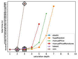
Figure 5. Total running time as the saturation depth is increased. Missing points indicate a time greater than the timeout of 90 seconds. For each benchmark, the depth that suffices for both the upper and lower bounds to be the ones given in Tab. 3 is marked by a larger, black marker of the same type as the line plot for the benchmark.

Fig. 5 shows how the overall time of AutoBound changes as the saturation depth is increased, using a timeout of 90 seconds (each data point averaged over 3 runs). We see that running time increases steeply, which is expected because the number of product terms grows exponentially with the saturation depth. We are pleasantly surprised by the fact that AutoBound tolerates even larger saturation depths for some of the benchmarks. However, saturation depth of 8 causes AutoBound not to terminate within the time limit in any of the benchmarks. Further data on the cone size and the run-time breakdown as the saturation depth is increased until a 10 minutes timeout appear in §8.

8. Detailed Statistics from Saturation Depth Experiment

Table 2. The size of the cone and run-time breakdown of each examples as the saturation depth is increased until a timeout of 10 minutes. #c-eq and #c-ineq are resp. the number of equalities/inequalities in the generated cone’s ideal/polyhedron; #m is the number of distinct monomials in the inequalities. time is the overall execution time of AutoBound (all times in seconds). csat is the time to saturate the cone. reduce is the time to reduce w.r.t. the cone using local projection. – indicates a timeout.

Benchmark		Saturation depth
		1	2	3	4	5	6	7
fixedPointInt	#c-eq	2	2	2	2	2	2	2
	#c-ineq	8	42	162	489	1281	2993	6425
	#m	9	41	131	336	742	1470	2682
	time	0.1	0.2	0.4	1.1	4.6	25.3	83.2
	csat	0.1	0.2	0.3	0.7	2.0	6.4	20.8
	reduce	0.0	0.0	0.1	0.4	2.5	18.9	62.4
manualPrice	#c-eq	4	4	4	4	4	4	4
	#c-ineq	7	43	163	492	1284	2999	6431
	#m	10	49	168	462	1092	2310	4488
	time	0.2	0.3	0.6	2.5	11.4	66.0	338.9
	csat	0.2	0.2	0.5	1.3	4.4	16.7	61.9
	reduce	0.0	0.0	0.1	1.2	7.0	49.3	277.0
manualPriceMonotone	#c-eq	8	8	8	8	8	8	–
	#c-ineq	8	53	218	712	1999	5001	–
	#m	11	60	228	690	1782	4092	–
	time	0.2	0.4	0.8	4.3	47.9	283.1	–
	csat	0.2	0.3	0.6	2.3	11.3	54.1	–
	reduce	0.0	0.1	0.2	2.0	36.5	229.0	–
tokent	#c-eq	13	13	13	–	–	–	–
	#c-ineq	12	90	815	–	–	–	–
	#m	12	71	288	–	–	–	–
	time	0.2	0.3	2.3	–	–	–	–
	csat	0.2	0.3	1.2	–	–	–	–
	reduce	0.0	0.1	1.0	–	–	–	–
nirn	#c-eq	16	16	16	–	–	–	–
	#c-ineq	21	322	4057	–	–	–	–
	#m	21	209	1351	–	–	–	–
	time	0.4	1.0	65.7	–	–	–	–
	csat	0.4	0.9	9.6	–	–	–	–
	reduce	0.0	0.1	56.1	–	–	–	–

The cone size and run-time breakdown of AutoBound as the saturation bound is increased in each benchmark, until a timeout of 10 minutes.

8.1. Bound Quality

Table 3. Comparison of the bounds that AutoBound generates for input term $t$ (saturation depth=3) and the bounds curated by a human expert. $\star$ indicates a result that is too large to include in the table. ed shows the (second component of the) effective-degree of the bound (the first component is 0).

Benchmark name	$t$	AutoBound		Expert
		bound	ed	bound	ed
elastic	$x-y$	$\leq{\frac{v}{e+a}}+1$	2	$\leq\left\lfloor\frac{v}{e+a}\right\rfloor+1$	2
		$\geq-1$	0	$\geq 0$	0
fixedPointInt	$\left\lfloor\frac{\left\lfloor\frac{ab}{\textit{sf}}\right\rfloor\cdot\textit{sf}}{b}\right\rfloor$	$\leq a$	1	$\leq a$	1
		$\geq a-1-\frac{\textit{sf}}{b}$	2	$\geq a-\frac{\textit{sf-1}}{b}$	2
manualPrice	$\textit{price}(\tilde{t})$	$\leq\textit{startPrice}$	1	$\leq\textit{startPrice}$	1
		$\geq\textit{minimalPrice}$	1	$\geq\textit{minimalPrice}$	1
manualPriceMonotone	$\textit{price}(\tilde{t}_{2})-\textit{price}(\tilde{t}_{1})$	$\leq 0$	0	$\leq 0$	0
token	$\textit{balanceJoined}-\textit{balanceSplit}$	$\leq 2$	0	$\leq 1$	0
		$\geq-1/2-1/2\cdot\textit{funds}$	1	n.a.	–
nirn	$\textit{shares1}-\textit{shares2}$	$\leq 1.88$	0	n.a.	–
		$\star$	5	n.a.	–

Tab. 3 presents the bounds we obtain for the benchmarks with saturation depth $3$, as well as the bounds generated manually by a verification expert (where available). $\star$ indicates that AutoBound has generated a bound we deem as uninformative. As explained in §4, there are potentially multiple optimal upper-bounds. Moreover, the technique can discover several upper bounds of the same effective-degree in one run of Alg. 1; in AutoBound we simply return multiple bounds in that case. In the table, this arose in fixedPointInt (5 upper bounds), where it was easily to select the most appealing of them (the other involving additional added terms); and NIRN (2 lower bounds), where both bounds were uninformative, as indicated in the table by $\star$. The latter case we discuss separately, below in §8.1.2.

8.1.1. Optimality

The bounds that AutoBound produces are nearly optimal w.r.t. the effective-degree order. The lower bound for elastic, and the upper bound for manual-price monotonicity, token, and NIRN are all constant, which is always optimal. The upper bounds for fixed point and manual price are also optimal, consisting merely of one variable. (These two results are optimal because there is no valid constant bound; moreover, there is no other bound consisting of a single variable that is valid.) It is harder to evaluate whether the remaining bounds are close to optimal w.r.t. the effective-degree order; however, they have the same effective-degree as the expert bounds, where the latter are available.

8.1.2. Desirability

As Tab. 3 demonstrates, the bounds that AutoBound computes match or nearly match the bounds produced by a domain expert, and differ in constant or nearly-constant (e.g. $\frac{1}{b}$) terms. We attribute these differences to the challenge of inequality reasoning inside a function, which we discussed in §2.

The lower bound for NIRN that AutoBound computes does not seem desirable; it is complex, with an effective degree of 5, four floor terms, and three levels of floor nesting. This result may indicate that a saturation bound larger than $3$ is necessary, but we believe that the ultimate cause is inequational assumptions that are present in the original code but are missing in our model (this was our experience with the token example and the NIRN upper bound).

8.1.3. Sufficient Saturation Depth

The smallest saturation bound that suffices to produce the bounds of Table 3 are marked on Fig. 5 using a larger marker of the same type is the other data points of the benchmark. All are below 3, and 2 suffices for some.

9. Related Work

Optimization modulo theories

Optimization modulo theories is the problem of minimizing (or maximizing) an objective function subject to a feasible region that is defined by a first-order formula (ST:2012; LAKGC:2014; BCGIJRST:2021). This paper investigates a variation of this problem, in which the desired result is a term rather than a value. Most work on optimization modulo theories is concerned with linear arithmetic. An exception is BCGIJRST:2021, which—similarly to our work–handles non-linearity by “linearizing” the problem. BCGIJRST:2021 incorporates a linear optimization modulo theories solver into an abstraction-refinement loop with an exact non-linear solver that generates lemmas on demand. In contrast, our method eagerly communicates lemmas between a linear solver and a cooporating (incomplete) non-linear solver (based on cones of polynomials).

Non-linear abstract domains

The set of cones can be seen as an abstract domain, in which elements are conjunctions of polynomial inequalities. In this sense, cones are analogous to convex polyhedra, which represent conjunctions of linear inequalities. Unlike the case of convex polyhedra, the concretization function that maps cones to their solutions is not injective; that is, “inequivalent” cones may represent the same set of points (e.g., the cones generated by $\{x,y\}$ and $\{x,xy\}$ are different, but the formulas $x\geq 0\land y\geq 0$ and $x\geq 0\land xy\geq 0$ represent the same points). The saturation steps (§5) can be conceived as semantic reduction (CC:1979): each saturation step derives new valid inequalities, while leaving the solutions to those inequalities unchanged.

There are a number of non-linear abstract domains that include semantic-reduction steps akin to cone saturation (KCBR:2018; BRZ:2005; GG:2008; CL:2005). The wedge abstract domain introduced in KCBR:2018 is most similar to our saturation step—it uses a combination of Gröbner-basis, congruence-closure, and polyhedral techniques for saturation. Unlike the wedge domain, this paper uses a systematic rather than heuristic method for applying the rule that the product of two non-negative polynomials is non-negative. In this regard, our method is similar to the domain of polynomial inequalities proposed in BRZ:2005, and the domain of of polynomial equalities proposed in (Colon:2004).

Positivstellensatz

In the case of real arithmetic positivstellensatz theorems (putinar; Schmudgen) give completeness results concerning which polynomials are positive given a set of inequality assumptions. They are the non-linear analogue of Farkas’ lemma. For Farkas’ lemma conical combinations by non-negative scalars is sufficient; however positivstellensatz theorems consider an ideal and conical combinations by more general terms; e.g. sum-of-squares polynomials in the case of putinar. In the Kriving–Stengle positivstellensatz, sum-of-squares polynomial combinations are taken with respect to products of the basis inequalities, which is similar to our process of taking products in §5.3. CHA:2020; FZJZX:2017 have both used positivstellensatz theorems with a degree bound in the context of program analysis by reducing to semi-definite programming, and consequently give numerical solutions. Our method does not perform such a reduction and can therefore easily give exact results. However, we lack an analogue of their completeness results.

References

- (1)
- Bagnara et al. (2005) Roberto Bagnara, Enric Rodríguez-Carbonell, and Enea Zaffanella. 2005. Generation of Basic Semi-Algebraic Invariants Using Convex Polyhedra. In Proceedings of the 12th International Conference on Static Analysis (London, UK) (SAS’05). Springer-Verlag, Berlin, Heidelberg, 19–34. https://doi.org/10.1007/11547662_4
- Bigarella et al. (2021) Filippo Bigarella, Alessandro Cimatti, Alberto Griggio, Ahmed Irfan, Martin Jonáš, Marco Roveri, Roberto Sebastiani, and Patrick Trentin. 2021. Optimization Modulo Non-linear Arithmetic via Incremental Linearization. In Frontiers of Combining Systems, Boris Konev and Giles Reger (Eds.). Springer International Publishing, Cham, 213–231.
- Buchberger (1985) Bruno Buchberger. 1985. Gröbner bases: an algorithmic method in polynomial ideal theory. Multidimensional systems theory, Progress, directions and open problems, Math. Appl., D. Reidel Publ. Co. 16, 184-232 (1985).
- Buchberger (1998) Bruno Buchberger. 1998. An Algorithmic Criterion for the Solvability of a System of Algebraic Equations (translated by Michael Abramson and Robert Lumbert). In Gröber Bases and Applications. Cambridge University Press.
- Chang and Leino (2005) Bor-Yuh Evan Chang and K. Rustan M. Leino. 2005. Abstract Interpretation with Alien Expressions and Heap Structures. In Verification, Model Checking, and Abstract Interpretation, Radhia Cousot (Ed.). Springer Berlin Heidelberg, Berlin, Heidelberg, 147–163.
- Chatterjee et al. (2020) Krishnendu Chatterjee, Hongfei Fu, Amir Kafshdar Goharshady, and Ehsan Kafshdar Goharshady. 2020. Polynomial Invariant Generation for Non-Deterministic Recursive Programs (PLDI 2020).
- Colón (2004) Michael Colón. 2004. Approximating the Algebraic Relational Semantics of Imperative Programs. In Static Analysis, 11th International Symposium, SAS 2004, Verona, Italy, August 26-28, 2004, Proceedings (Lecture Notes in Computer Science, Vol. 3148), Roberto Giacobazzi (Ed.). Springer, 296–311. https://doi.org/10.1007/978-3-540-27864-1_22
- Cousot and Cousot (1979) Patrick Cousot and Radhia Cousot. 1979. Systematic Design of Program Analysis Frameworks. In Proceedings of the 6th ACM SIGACT-SIGPLAN Symposium on Principles of Programming Languages (San Antonio, Texas) (POPL ’79). Association for Computing Machinery, New York, NY, USA, 269–282. https://doi.org/10.1145/567752.567778
- Cox et al. (2015) David A. Cox, John Little, and Donal O’Shea. 2015. Ideals, Varieties, and Algorithms (4 ed.). Springer.
- de Moura and Bjørner (2008) Leonardo de Moura and Nikolaj Bjørner. 2008. Z3: An Efficient SMT Solver. In Tools and Algorithms for the Construction and Analysis of Systems (TACAS).
- Faugère (1999) Jean-Charles Faugère. 1999. A new efficient algorithm for computing Gröbner bases (F4). Journal of Pure and Applied Algebra (1999).
- Faugère (2002) Jean-Charles Faugère. 2002. A New Efficient Algorithm for Computing Gröbner Bases without Reduction to Zero (F5). In Proceedings of the 2002 International Symposium on Symbolic and Algebraic Computation (ISSAC ’02).
- Faugère (2010) Jean-Charles Faugère. 2010. FGb: A Library for Computing Gröbner Bases. In Mathematical Software – ICMS 2010.
- Feng et al. (2017) Yijun Feng, Lijun Zhang, David N. Jansen, Naijun Zhan, and Bican Xia. 2017. Finding Polynomial Loop Invariants for Probabilistic Programs. In Automated Technology for Verification and Analysis, Deepak D’Souza and K. Narayan Kumar (Eds.). Springer International Publishing.
- Flanagan and Qadeer (2002) Cormac Flanagan and Shaz Qadeer. 2002. Predicate Abstraction for Software Verification. In Proceedings of the 29th ACM SIGPLAN-SIGACT Symposium on Principles of Programming Languages (POPL ’02). https://doi.org/10.1145/503272.503291
- Gulavani and Gulwani (2008) Bhargav S. Gulavani and Sumit Gulwani. 2008. A Numerical Abstract Domain Based on Expression Abstraction and Max Operator with Application in Timing Analysis. In Proceedings of the 20th International Conference on Computer Aided Verification (Princeton, NJ, USA) (CAV ’08). Springer-Verlag, Berlin, Heidelberg, 370–384. https://doi.org/10.1007/978-3-540-70545-1_35
- Isermann (1982) H. Isermann. 1982. Linear lexicographic optimization. Operations-Research-Spektrum 4 (1982). Issue 4.
- Kincaid et al. (2018) Z. Kincaid, J. Cyphert, J. Breck, and T.W. Reps. 2018. Non-Linear Reasoning for Invariant Synthesis. PACMPL 2(POPL) (2018), 54:1–54:33.
- Komuravelli et al. (2016) A. Komuravelli, A. Gurfinkel, and S. Chaki. 2016. SMT-Based Model Checking for Recursive Programs. In Formal Methods in System Design. https://doi.org/10.1007/s10703-016-0249-4
- Li et al. (2014) Yi Li, Aws Albarghouthi, Zachary Kincaid, Arie Gurfinkel, and Marsha Chechik. 2014. Symbolic Optimization with SMT Solvers. SIGPLAN Not. 49, 1 (jan 2014), 607–618. https://doi.org/10.1145/2578855.2535857
- Loos and Weispfenning (1993) R. Loos and V. Weispfenning. 1993. Applying Linear Quantifier Elimination. Comput. J. 36 (1993).
- Putinar (1993) Mihai Putinar. 1993. Positive Polynomials on Compact Semi-Algebraic Sets. Indiana Univ. Math. J. 42 (1993), 969–984. Issue 3.
- Schmüdgen (2017) Konrad Schmüdgen. 2017. The Moment Problem on Compact Semi-Algebraic Sets. Springer International Publishing, 283–313. https://doi.org/10.1007/978-3-319-64546-9_12
- Sebastiani and Tomasi (2012) Roberto Sebastiani and Silvia Tomasi. 2012. Optimization in SMT with () Cost Functions. In Automated Reasoning, Bernhard Gramlich, Dale Miller, and Uli Sattler (Eds.). Springer Berlin Heidelberg, Berlin, Heidelberg, 484–498.