smectic -model
Abstract
A unidirectional “density” wave order in an otherwise isotropic environment is guaranteed to display smectic-like Goldstone mode. Examples of such “soft” states include conventional smectic liquid crystals, putative Fulde-Ferrell-Larkin-Ovchinnikov superfluids, and helical states of frustrated bosons and spins. Here we develop generalized spin-smectic -models that break internal symmetry in addition to the -dimensional rotational and uniaxial translational symmetries. We explore long-wavelength properties of such strongly fluctuating states, show that they are characterized by a “double-power-law” static structure peak, and analyze their asymptotic symmetry-reduced crossover to conventional low-energy modes. We also present the associated Ginzburg-Landau theory, describing phase transition into such spin-smectic states, and discuss experimental realization of such models.
I Introduction
I.1 Background and motivation
There are number of systems in nature that spontaneously undergo transitions to a variety of “density” 111Throughout the manuscript we will use the term “density” to also refer to spin, Cooper pair, and other generalized densities that transform nontrivially under internal symmetry. wave states, characterized by a periodic modulation. Such systems range from a large variety of charge and spin density waves, e.g., antiferromagnetic insulators in cuprates [2], charge density waves in [3] and Wigner crystal [4], to the putative pair-density wave superconductors [5]. Generically, in an orientationally-ordered environment of a crystal, the low-energy nonlinear -model (nm) description of the corresponding Goldstone modes is given by their linear gradient elasticity, at weak coupling controlled by a Gaussian fixed point, and is thus quite well-understood [6, 7, 8, 9, 2, 10].
In contrast to these systems, there exists a qualitatively distinct class of phases of matter, where a unidirectional density-wave order (characterized by a spontaneously-oriented wavevector ) takes place in an isotropic environment, and thus, in addition to translational and internal symmetries, also spontaneously breaks spatial rotational symmetry. We expect such states to be described by a “soft” – higher gradient – nm that is qualitatively distinct from their crystalline counterparts. The derivation and study of such models are the focus of the present work.
The simplest realization of such states is the extensively-studied conventional smectic liquid crystals [11] characterized by a periodic scalar number-density, described by a fully rotationally-invariant soft nonlinear elastic model [12, 13]. In the presence of thermal and quantum fluctuations or quenched disorder [14, 15, 16], the corresponding scalar phonon (denoted as ) fluctuations are qualitatively enhanced (e.g., for spatial dimension , thermal grows with system size, diverging in the thermodynamic limit) and lead to importance of the nonlinear elasticity [12], resulting in a tuning-free critical smectic phase described by universal exponents [17].
In this paper, we consider a generalization of such a scalar smectic to “spin” (non-scalar) density, , that transforms nontrivially under -spin rotational symmetry. Such a state, that we dub “spin-smectic”, is characterized by an internal flavor degrees of freedom, and exhibits a spontaneous uniaxial spatial modulation in along . It thereby spontaneously breaks the -internal spin symmetry, and the underlying spatial -rotational and -translational symmetries.
Our study of such spin-smectics is motivated by a number of physical realizations of unidirectional orders, that include: (i) : conventional smectic liquid crystal [11], and quantum Hall striped states of a two-dimensional electron gas at half-filled high Landau levels [18, 19, 20, 21, 22, 23], (ii) : cholesteric liquid crystal [24], spin-orbit coupled and dipolar Bose condensates [25, 26], putative Fulde-Ferrell-Larkin-Ovchinnikov (FFLO) paired superfluids [27, 28] in imbalanced degenerate atomic gases [29, 30], a -wave resonant Bose gas [31, 32], and helical states of frustrated bosons [33], (iii) : helimagnets of frustrated spin systems 222These are distinct from another interesting class of helimagnets arising from the chiral Dzyaloshinskii-Moriya (DM) spin-orbit interaction that drives the helical structure. Such DM helical states are less symmetrical than those considered in this paper, and do not exhibit independent and symmetries. In such systems, equivalent to a cholesteric liquid crystal the orientations of and are locked, and thus at low energies its Goldstone mode reduces to that of a smectic, as discussed in Ref. [24]. Physical realizations of such system include MnSi, which is an itinerant ferromagnet exhibiting helical structure at low temperatures. These systems show anomalous magnetic [50, 51, 52] and transport [53] behavior as probed over different temperature, pressure, and magnetic field. [35, 36], as realized in spinel materials, e.g., [37, 38] and [39], van der Waals honeycomb magnets, e.g., [40], and stretched diamond lattice, e.g., [41]. For long wavelength (lattice constant) spin-density modulation, even in the crystalline realizations with spin-orbit interactions above, we expect the spin-smectics to emerge in a broad range of intermediate scales from an approximate rotationally-symmetric state, even if asymptotically crossing over to more conventional ordered states.
I.2 Frustrated spin model
Before we summarize our main findings, we discuss the frustrated lattice model, studied at a microscopic level in Refs. [35, 36]. The long-scale phenomenology that emerges from this model motivates our current study.
Its Hamiltonian is given by
| (1) |
where is an -component spin on site (with respectively corresponding to the Ising, XY, and Heisenberg models), and denote the nearest-neighbor (NN) and next-nearest-neighbor (NNN) pairs of sites. The frustration of the system is then induced by the antiferromagnetic NNN interactions, , while the sign of the NN exchange interactions is not important (as it is nonfrustrating and can be changed by a bipartite transformation), but for concreteness and convenience we take to be . Then, the spin frustration is characterized by the ratio, . In the classical limit the model (1) exhibits ground state degeneracy. Taking the diamond-lattice antiferromagnets (as realized in AB2X4 compounds with A a magnetic ion living on a diamond lattice and B living on a pyrochlore lattice, studied by Bergman et al. [35]) for example, for weak frustration, , the ground state is the Nel state. For intermediate frustration, , the ground state is an incommensurate helical spin-density wave that is degenerate with respect to orientation of the ordering wavevector on the so-called spiral codimension one surface around the point. For , the spiral surface exhibits open topology along the axis, and in the limit , collapses into one dimensional lines that correspond to the nearest-neighbor-coupled face-centered cubic antiferromagnet.
As a consequence of the large classical ground-state degeneracy, the ordering temperature, , is small relative to the Curie-Weiss exchange scale, [42]. For example, spinel compounds like [37, 38] and [39] have and , respectively. This is considered as empirical signatures of highly frustrated magnets. As an aside, this then leads to a broad regime of spiral classical spin liquid for temperatures , where the system thermally explores many different low-energy configurations on the spiral surface and thereby exhibit anomalous physical properties. This is in contrast with an even more exotic quantum spin liquid that survives down to zero temperature [43].
At low temperatures, , the ordering of such magnets is associated with the lifting of the spiral surface degeneracy that is sensitive to the degeneracy-breaking perturbations like spin-orbit and crystalline symmetry breaking anisotropies. In the absence of such perturbations, the spiral surface degeneracy is lifted via quantum and thermal fluctuations in the free energy, which select a set of wavevectors (whose magnitude is given by the radius of spiral surface, ) of the ordered states that one expects to be along the crystalline symmetry axes – the so-called order-by-disorder [44, 45]. The resulting low-temperature ordered phases range from the nematic [36] to a variety of spin-density-wave states at specific wavevector [35]. The ordering of the latter self-consistently introduces a stabilizing stiffness of a conventional nm and thereby determines other physical observables such as the specific heat and structure factor [35, 33]. As a result, the fluctuation-generated stiffness is small, subdominant to the higher order gradient elasticity over a large regime (set by order-by-disorder scale), within which the system exhibits the softer (than conventional spin-density-wave states) smectic-like elasticity [33]. Our goal here is to study the universal low-energy description and phenomenology of such soft, unidirectionally ordered spin-density-wave states, that we refer to as spin-smectics. To this end, in this paper we primarily focus on an isotropic (i.e., neglecting the order-by-disorder and lattice symmetry breaking effects) field theory controlled by the ordering on the spiral momentum surface.
I.3 Results
| Coplanar | Collinear | |
| N/A | ||
| + | ||
| soft nm, (2) | + , (4) |
I.3.1 Coplanar smectic -model
Motivated by the above physical systems and the frustrated Heisenberg model [35, 36], generalized to spin components, our key result (summarized for different cases of interest in Table 1) is the derivation of smectic -model for -component orthonormal diad, described by the Hamiltonian density
| (2) |
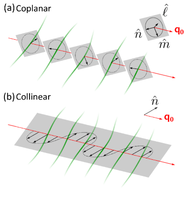
It describes the nonlinear Goldstone modes of the coplanar spiral state at a wavevector [see Fig. 1(a)]. In the above, we defined components of spin fluctuations transverse to the spiral plane and the complex vector . For simplicity of presentation here, we neglected inessential (quantitative) anisotropy in , discussed in the main body of the paper. Throughout this paper, we use the subscripts () and to denote the axes parallel and perpendicular to , respectively. The modulus describes the “soft” Goldstone-mode elasticity for the fluctuations in the plane, which for weak excitations reduces to the standard smectic form, (33), and also introduces stiffness for . The terms give linear-gradient elasticity for the out-of--plane fluctuations. We find that , , predicting a divergent anisotropy near the critical point, where .
For the special case of , the spin-smectic -model in (2) reduces to
| (3) |
where the complex -vector , defining an orthonormal triad .
Easy-plane (XY) anisotropy locks along the anisotropy axis , reducing the model to a conventional smectic -model, of e.g., cholesteric and Fulde-Ferrell states for with .
I.3.2 Collinear smectic -model
For collinear spiral states [see Fig. 1(b)], the low-energy Goldstone modes are a smectic-like pseudo-phonon corresponding to the spin-density wave phase and a unit vector that describes local spin orientation. These are characterized by a Hamiltonian density
| (4) |
where is the rotationally-invariant strain tensor. In the presence of easy-axis anisotropy common to magnetic crystalline materials, when , the spin orientation freezes out, leading to low-energy smectic -model described by a single smectic phonon derived in Sec. II.1. When , the spin orientation is locked perpendicular to , resulting in an collinear smectic, such as the Larkin-Ovchinnikov state.
I.3.3 Thermal fluctuations and structure factor
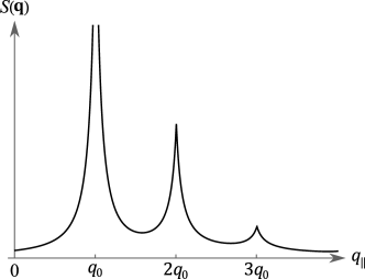
Focusing on the physical case, , we show that both the coplanar and collinear states are described by a smectic phonon and two Goldstone modes at the harmonic level, i.e., at the Gaussian fixed point, neglecting effects of nonlinearities that may lead to a crossover to a nontrivial spin-smectic fixed point, thereby modifying these predictions at long scales. Accordingly, they both exhibit quasi-long-range and long-range orders in their spin-density modulation and spin orientation orders, respectively. As illustrated in Fig. 2, this then leads in 3d to anisotropic double-power-law peaks in their static spin structure factor at () [see Eq. (III.4) for a more detailed form],
| (5) |
where ()
| (6) |
with the positive temperature-dependent exponent . In the above, the first term is the leading (narrower) smectic Goldstone mode contribution of the power-law peak, while the second term is the sub-leading (broader) contribution from the Goldstone mode fluctuations, with the prediction valid at small , expected to become important as this ratio becomes of order or larger.
We discuss the effects of various symmetry-breaking perturbations that exist in real materials, including the lattice anisotropy and spin-orbit coupling. The former breaks the spatial rotational symmetry, and thereby leads to a crossover for the smectic phonon mode to XY correlation (see Fig. 5). This results in true Bragg peaks (delta functions), as in conventional long-range-ordered states, but may keep the power-law tail at intermediate scales if the symmetry-breaking perturbation is weak. On the other hand, the spin-orbit coupling, as e.g., Dzyaloshinskii-Moriya (DM) interaction in a helimagnet (or a chiral twist term in a cholesteric), breaks symmetries down to the diagonal subgroup. For the coplanar state, this locks the orientation of perpendicular to , and thereby freezes out the two XY Goldstone modes, resulting in single-power-law peak with the second term in (6) suppressed.
I.3.4 Transition into the spin-smectic: de Gennes model
To describe the criticality associated with the phase transition into these spin-smectic states, illustrated in Fig. 3, we also derive a generalized de Gennes model [11], with Hamiltonian density given by,
| (7) |
where the complex vector ( and are independent -vectors, physical cases corresponding to ) describes the spin-density wave order parameter, and with a spatial unit vector that describes the translationally invariant nematic liquid that spin-smectic melts into for . This Ginzburg-Landau theory, which we dub spin-de Gennes model, at low-temperatures for predicts the collinear () and coplanar () states discussed above.
I.3.5 Quantum dynamics
By including the Wess-Zumino-Witten Berry phase, that encodes the spin precessional dynamics and corresponding spin commutation relations, we supplement above classical smectic -models with quantum dynamics in the spin-coherent path integral. For coplanar state we find that Berry phase action for the smectic -model is given by a
| (8) |
where is the uniform ferromagnetic susceptibility in the coplanar phase.

The remainder of the paper is organized as follows. In Section II, we derive the continuum field theory of the lattice model (1) with generalized spin symmetry and the underlying spatial rotational and translational symmetries. It gives our key result, a new class of “soft” -models that describe the universal long-wavelength properties of spin-smectics. We show that these reduce to the fully nonlinear Goldstone-mode field theories for the conventional smectic liquid crystals (), the putative FFLO paired superfluids in imbalanced degenerate atomic gases (), and a new class of soft-spin-density waves (), among other physical realizations. In Section III, we analyze the spin-smectic in the presence of weak thermal fluctuations, assess its stability, and compute its correlation functions, focusing on the structure factor that exhibits crossovers across a range of length scales. In Section IV, we introduce a complementary Ginzburg-Landau model that gives spin-smectic as its ordered state and describes the transition from the orientationally ordered to the spin-smectic states. In Section V, starting with the WZW term we derive the quantum dynamics for the spin-smectic -model. We conclude in Sec. VI with a summary of our results and a discussion of open directions.
II Field theory of smectics
The key feature of the frustrated lattice model, (1), is its degenerate ground-state manifold (neglecting order-from-disorder effects), defined by a spiral surface , where is the wavevector of the spin spiral state. Motivated by this class of models and corresponding experimental realizations of frustrated helimagnets [37, 38, 39, 40, 41], we develop the field theory of low-energy excitations of helical states that emerge from an isotropic spiral surface, , neglecting spin-orbit coupling (SOC) and rotational-symmetry-breaking lattice effects. To this end, we develop an Goldstone-mode -model by starting with an -component spin model with Hamiltonian density (throughout this paper, we employ the Einstein convention, where repeated indices are implicitly summed over),
| (9) |
that encodes the coplanar and collinear spiral states on a hyper-spherical spiral surface, , that can be derived from the microscopic Hamiltonian (1). We note that the Hamiltonian (II) respects -rotational (and -translational with the spatial dimension) symmetry, neglecting any SOC, i.e., forbidding the inner product between the spatial () and “spin” () degrees of freedom.
Driven by the term, that for clearly exhibits a nonzero momentum spin condensation on an -symmetric spiral surface 333Generally, the wavevector that minimizes the energy , as it can be corrected by other (than ) gradient terms and higher-order fluctuations., we consider (as we will show, most strongly-fluctuating) unidirectional, single spin states 444We do not consider mutli-, nor non-Landau spin liquid states [43]. Determining the true ground state among the single- and these states is a challenging microscopic question that falls outside of effective field theory approach taken here and is best addressed numerically.
| (10) |
where and are -component real vector fields, that can be compactly written as a complex -vector field
| (11) |
with degrees of freedom.
The remaining quadratic and quartic terms in (II) for encode Landau ordering and determine the amplitude of the spin-density-wave spiral. We note that in contrast to conventional Landau theories, here the ordering is at a nonzero wavevector, with condensing at a nonzero momentum . Therefore, the higher derivative terms play an important role, as they constitute the lowest-order form needed for a generic Goldstone-mode description of the spin-smectic -model 555On this account, higher order gradient quartic-in- terms can be included, but add nothing new beyond those already included in (II), which is the minimum form required for a generic description, as we verify a posteriori.. As we will show, the in (II) are crucial for the stabilization of the spin-density waves.
With the ansatz (II), the mean-field (constant part, after dropping the fast-oscillating contributions, that on spatial integration average out to zero) energy density is given by
| (12) |
where the zeroth-order couplings (corrected by fluctuations) are given by
| (13) |
At low temperatures, (and ), the spin-density wave is ordered and can be parametrized as
| (14) |
where and are, respectively, the overall and relative amplitudes of order parameters and . The (mean-field) magnitude of the ordering wavevector is then determined by minimizing the Landau free energy (12), with direction chosen spontaneously. For we find,
| (15) |
It is straightforward to see that the Landau theory (12) predicts two qualitatively distinct spin-density waves. With the parametrization (14), the quartic interaction can be written as
| (16) | ||||
| (17) |
For (or ), it is clearly minimized by
| (18) |
with arbitrary phase, . This allows us to rewrite the order parameter as
| (19) |
where the minimization of (12) then gives,
| (20) |
The resulting collinear spin-density wave (II) is then given by oscillatory magnitude,
| (21) |
In contrast, for (and ), minimization of (17), then gives,
| (22) |
where is an arbitrary integer. This gives a coplanar, i.e., helical spin-density-wave state characterized by the order parameter
| (23) |
with a constant magnitude
| (24) |
given by
| (25) |
Importantly, because of the absence of SOC both the collinear and coplanar states have decoupled spin orientation and wavevector , particularly distinguishing the coplanar state from the helical state of a DM helimagnet and a cholesteric state of a chiral liquid crystal.
Based on the above analysis, below we first derive -models for the cases of , which, as we will show correspond to the familiar ordered states of a conventional smectic and the putative Fulde-Ferrell-Larkin-Ovchinnikov (FFLO) superfluids, respectively. We then study the case (and its generalization to larger ), corresponding to collinear and coplanar spin-density waves, described by two distinct “soft” nonlinear smectic -models. These are relevant to the ordered states of “codimension one” frustrated magnetic systems reviewed in Sec. I.2.
II.1 : conventional smectic
We begin with the simplest case of , corresponding to a scalar number density , that according to field theory (II) condenses into a scalar-density wave,
| (26) |
where , with smectic amplitude and the phonon Goldstone mode, corresponding to the displacement along , familiar from conventional smectic liquid crystals. In our generalized formulation this state corresponds to a necessarily collinear case, with one-component “vectors” , parametrized by and .
At low temperatures in the ordered smectic state, the amplitude is well approximated by a mean-field value
| (27) |
with only small gapped fluctuations. Thus, with the ansatz (II.1) and its derivatives
| (28) |
the model (II) (neglecting and that are unimportant for ) reduces to the familiar nonlinear smectic Goldstone-mode elasticity,
| (29) |
where in the first equality, we dropped fast oscillating pieces, that average away after spatial integration of the energy density. Above, the rotationally-invariant strain tensor is
| (30) |
and two independent elastic constants and , at zeroth order (i.e., model (II) dependent) are given by,
| (31) |
The minimization of the constant part of ,
| (32) |
over and , gives , that ensures the vanishing of the coefficient of the linear in the strain term, and thereby guarantees the stability of the smectic state. We note that with the inclusion of fluctuations, the optimum wavevector gets corrected, i.e., , so as to eliminate the linear in contribution order by order (akin to what’s done with the order parameter ), which amounts to ensuring that the expansion in the nonlinear strain is done around the correct (fluctuation-corrected) ground state. With this, by choosing , we then recover the familiar nonlinear elastic, fully rotationally invariant smectic Goldstone-mode -model,
| (33) |
We observe that the emergence of smectic elasticity (33) is expected, based on spatial rotational symmetry encoded in (II), that requires a fully rotationally invariant nonlinear strain tensor . To see this we note that the global rotation of the undistorted smectic state is characterized by a rotation of ,
| (34) |
which corresponds to the phonon displacement
| (35) |
Using inside (33), straightforward analysis then shows that the nonlinear strain and thereby the energy (33) indeed vanishes under such rotation, i.e., .
More generally, the global rotation of the smectic state (34) is equivalent to the following transformation of :
| (36) |
as can be seen from its identification with the corresponding phase transformation of in Eq. (II.1). The latter transforms the nonlinear strain tensor
| (37) |
and thereby leaves the form of Hamiltonian (33) unchanged with rotated to , i.e., .
II.2 : XY smectic and FFLO/PDW superfluid
For , in its ordered regime the Hamiltonian (II) encodes a soft planar spin-density wave of XY spins. Physically, this is relevant for frustrated magnetic systems with an easy plane anisotropy and “striped” (e.g., Pair-Density Wave (PDW), FFLO, and other) nonzero-momentum superfluids [30]. The latter is characterized by a complex field, whose real and imaginary parts are isomorphic to a two-component real vector field. The symmetry of the superfluid then maps to the spin-rotational symmetry of the spin-smectic. Below, we show that the putative FF (time-reversal-breaking, amplitude uniform) and LO (time-reversal-preserving, amplitude modulated) PDWs states are isomorphic to the coplanar and collinear spin-density waves, emerging from the field theory, respectively.
The low-energy properties of a striped superfluid can be qualitatively captured by the following order parameter
| (38) |
where the two complex scalar fields,
| (39) |
distinguishing between the coplanar and collinear (i.e., the so-called FF and LO) states. The imaginary and real parts of the two complex order parameters in (38) can equivalently be encoded in a spin language, via two real two-component vectors via
| (40) |
where
| (41) |
with the superscripts and respectively denoting the real and imaginary parts of the corresponding complex fields.
As in the analysis of the previous subsection, here too the two phases are controlled by the sign of . For , the Landau free energy (12) selects the collinear state that satisfies the conditions (18) that together with (II.2) gives . The order parameter (38) then reduces to the familiar LO state
| (42) |
where the phases
| (43) |
are the LO superfluid phase and its smectic phonon, respectively. In terms of the two-component vector order parameters (40), this corresponds to the collinear case with
| (44) |
As detailed below and in Ref. [30], after choosing the minimum and dropping constants, the -model (4) reduces to the Goldstone mode Hamiltonian given by the coupled smectic and XY sectors [29, 30],
| (45) |
where . Notice that vanishes when the current-current interaction, (see below and Ref. [30]). Namely, it is required to capture the universal low-energy Goldstone-mode energetics of the LO state.
For , the Landau free energy (12) is minimized by the coplanar state that satisfies the conditions (22), that together with (II.2) gives and , which is equivalent to or . Thus, the order parameter (38) reduces to the FF state
| (46) |
where and amplitude is uniform. In terms of the vector order parameter (40), this corresponds to the coplanar state, with orthogonal vectors
| (47) |
Thus, the Goldstone-mode -model is described by a single smectic phonon (see below and Ref. [30])
| (48) |
where .
We next turn to the discussions of the coplanar -symmetric density-wave, which leads to a new class of soft nonlinear -model.
II.3 coplanar smectic
For the coplanar helical state, which satisfies the condition (22) and , the order parameter can be written as
| (49) |
where
| (50) |
is a complex N-component vector field with , described by orthonormal real vectors, and .
To count the number of Goldstone modes, we first note that the group consists of generators of rotation that correspond to independent planes in the -dimensional spin space. For an ordered state that breaks the entire group, there will be Goldstone modes. For the coplanar state, the symmetry group of the order parameter is (due to the subtraction of and axes). The Goldstone modes then live on manifold with Goldstone modes 666Alternatively, we can consider orthonormal basis vectors of the spin space: , , and (). The generators of rotation that act on the orthonormal diad correspond to the , , and planes. This then leads to Goldstone modes that live on the compact manifold, with and (for a given choice) corresponding to the rotations of and , respectively.
To derive the Goldstone-mode classical Hamiltonian of the coplanar state, we substitute (49) into (II) and first consider the simplest case with , which gives (see details in Appendix A)
| (51) |
where the zeroth-order parameters above are given by
| (52) |
By selecting to eliminate the (first) term in the Hamiltonian above, and expressing the result in terms of the orthonormal triad, we obtain:
| (53) |
We stress that this nonlinear -model is fully rotationally invariant for an arbitrary large spin-smectic layers rotation , corresponding to , where in 3d with any of the axes transverse to . With the definition of the order parameter (49), this rotation can be interpreted as the following transformation of and :
| (54) |
where . Thus, in the helical state the global spatial rotational symmetry of (II) maps onto an inhomogeneous spin rotational symmetry . It can be straightforwardly verified that the transformation (II.3) leaves the form of the Hamiltonian (53) unchanged with the axis rotated to .
II.3.1
To further analyze the Hamiltonian (53), we first consider the case of and parametrize the orthonormal diad as
| (55) |
corresponding to
| (56) |
where the angle is related to the phonon mode along by . The Hamiltonian (53) then describes a smectic phonon and reduces to (48) at low-energies, where the perpendicular stiffness of vanishes, consistent with our discussion of FF superfluid. As we will see, for a general , the soft smectic elasticity, enforced by the underlying spatial rotational symmetry, manifests as a vanishing perpendicular stiffness, , corresponding to inhomogeneous spin rotations in the plane.
II.3.2
Now we consider coplanar spin state. The spin space is now spanned by the orthonormal triad , , , where
| (57) |
with
| (58) |
Notably, the coplanar smectic -model can be expressed in terms of the following “spin connections”:
| (59) |
where and are real and complex spatial vector fields, respectively. To this end, we first note that an arbitrary vector in spin space, , can be expanded in terms of the orthonormal triad,
| (60) |
This enables us to express the linear gradient term in (53) as
| (61) |
where we used
| (62) |
In the above, the (first) and (second) terms correspond to the elastic moduli for the along- distortions of in-plane (one) and out-of-plane (two) polarizations, respectively. An important feature of the Goldstone-mode -model (53) is a vanishing of its transverse stiffness, , guaranteed by the underlying rotational symmetry of (II), corresponding to rotation of . The latter demands a vanishing of the curvature in the transverse component to in the thermodynamic potential. The vanished stiffness then follows from the equivalence of the infinitesimal shift and the following transformation:
| (63) |
In contrast, the vanishing of the transverse stiffness for the out-of-plane polarization , i.e., a modulus for in (53) is nonuniversal, unconstrained by any symmetry, and is accidental due to a non-generic (fine-tuned) nature of (II) for vanishing .
We next derive and analyze a generic coplanar smectic -model, by now including nonzero , . In particular, we show that introduces a nonzero stiffness for , controlling the out-of---plane fluctuations, leading to our universal Goldstone-mode -model of the helical state. This stiffness is also necessary to stabilize model (53), which is otherwise unstable against thermal fluctuations in any dimension (see Sec. III). A complementary view on the importance of the coupling and the presence of in the Goldstone mode theory is given in Appendix C.
To this end, we examine the contribution of nonzero in (II) to the -model in the coplanar helical state. Relegating the details to Appendices A and B, using the helical order parameter (49), dropping the oscillatory and constant contributions, we find,
| (64) |
where in the last line, we only kept terms up to quadratic order in and . At the minimum of the thermodynamic potential, we remove the linear in term with the rotationally-invariant strain tensor
| (65) |
which ensures the stability of the coplanar smectic state. This then leads to the correction,
| (66) |
with the sought-after stabilizing stiffness
| (67) |
Thus, by including the crucially stabilizing contribution to (53), we now have obtained the generic form of the smectic -model of the helical state, as advertised in the Results subsection of the Introduction, I.3,
| (68) |
where we included the stiffness, that, as we have seen above, is already contained in the contribution in (II.3.2) and can also be generated by other higher-order (in ) terms. Neglecting higher-derivative contributions in of (68) an equivalent, smectic form of the -model, expressed in terms of the “gauge” fields is given by
| (69) |
where the dimensionless field (not unit vector, )
| (70) |
leads to a conventional smectic form (33) for small angle fluctuations. In the above, the leading contributions to the zeroth-order parameters are
| (71) |
constrained to be () for stability of the coplanar helical state.
We close this helical state derivation by noting that term in (II) gives a contribution proportional to
| (72) |
where we used and . Since it is proportional to an already present term in (II), it simply shifts the minimum while leaving the form of the resulting Goldstone mode theory (53) unchanged.
Finally, we observe that, in contrast to the stabilizing tensor quartic operator in (II.3.2), a scalar quartic term, does not introduce any new physics into the helical -model, (68), (II.3.2). To see this, observe that in the helical state,
| (73) |
where in the second line, we only kept the terms up to quadratic order in . Thus, this contribution simply shifts the condition on that eliminates the first term in (51), only leaving the following correction to the smectic phonon elasticity,
| (74) |
Thus, the only consequence of this scalar quartic contribution (73) is to modify above zeroth-order (non-generic) expressions for , and , and in particular shows that the elastic constants and are independent.
II.3.3
For , the spin space is spanned by orthonormal vectors , and (). The (quadratic in and ) correction by the term, which for is given by (66), becomes
| (75) |
where . It now gives the following stabilizing out-of-plane contribution to the -model,
| (76) |
where in the last line we expressed it in terms of , the components of out-of-plane fluctuations defined in (58), using the identity
| (77) |
Thus, as advertised in the Results subsection of the Introduction, I.3, the smectic -model is given by
| (78) |
When higher-order gradients are neglected, it reduces to a form resembling a conventional smectic
| (79) |
II.4 collinear smectic
We next derive the Goldstone-mode smectic -model for the collinear state for a general . As discussed in Sec. II, the order parameter of the collinear state can be parametrized as
| (80) |
with
| (81) |
described by a unit “polarization” vector, , and a phonon mode, , with a parametrization redundancy that requires identification of with , which is already accounted for by . There are thus Goldstone modes living on the compact manifold. We also note that (in contrast to the coplanar state) the magnitude of such linearly-polarized spin-density wave state oscillates in space, and thus (81) corresponds to a coarse-grained spin-density order parameter.
We can now derive the collinear smectic -model using the representation (80) inside the piece of in (II). Relegating technical details to Appendix A, we obtain
| (82) |
where , the familiar nonlinear smectic strain is given by (30), and the zeroth-order elastic moduli are
| (83) |
We note that, as expected on general symmetry grounds, at the energy minimum , the phonon mode is “soft” (i.e., controlled by higher derivative elasticity), with a vanishing transverse-to- stiffness, . This is enforced by the underlying rotational invariance of in (II) (including fluctuations), which corresponds to an arbitrary rotation of the spontaneously chosen . This then ensures the vanishing of the transverse-to- curvature in the thermodynamics potential at the minimum , with the zero stiffness that then follows from the equivalence of the following transformations,
| (84) |
where , coming from the definition of the order parameter in (80).
In contrast, the vanishing of the transverse stiffness of the Goldstone mode is a purely accidental property of the term in (II), and is generically expected to be nonzero for the full . Indeed, by including the term (with details given in Appendix A), we find
| (85) |
which gives a nonzero transverse stiffness for gradient deformations. With this, and choosing , we finally obtain the collinear smectic -model for its Goldstone modes,
| (86) |
where the zeroth-order stiffnesses are given by,
| (87) |
Neglecting symmetry-allowed nonlinearities in and ,
| (88) |
leads to two decoupled sectors of a conventional scalar smectic in and the standard -model in (4). We leave the open question of the effects of these coupling to a future study. Other term like also gives a corrections to (proportional to ), but does not change the universal long-wavelength form (II.4). As expected, for , the Hamiltonian density (II.4) reduces to the smectic -model of the LO superfluid, (45), with the superfluid phase representing the single Euler angle of , corresponding to the complex superfluid order parameter.
III Thermal fluctuations in the smectic states
Having established the corresponding smectic coplanar and collinear -models, we next analyze the thermodynamic properties of these smectic spin-density wave states, with a focus on the physical case of . We limit our analysis to classical statistical mechanics at the Gaussian fixed point, with the Goldstone-modes partition function given by,
| (89) |
where ( throughout) and given by (50) and (81) for the coplanar and collinear states, respectively.
Namely, below we introduce the angular fields representation of the Goldstone modes in the Hamiltonian density for these two smectic states. Then, we examine their stability to small thermal fluctuations within a Gaussian approximation, followed by a discussion of possible consequences of the nonlinearities and symmetry-breaking perturbations. We will then calculate Goldstone modes’ correlation functions that control low-energy, long-wavelength scattering and thermodynamics.
III.1 Angular representation of Goldstone modes
III.1.1 Collinear state
As discussed in the previous sections, the collinear smectic state (80) is characterized by a smectic phonon and a unit spin vector . The latter can be parameterized by
| (90) |
where we chose an orthonormal frame , , , such that for small fluctuation of these angular Goldstone modes, and ,
| (91) |
Neglecting higher-order gradients, the Hamiltonian density (II.4) is then given by
| (92) |
III.1.2 Coplanar state
The fluctuations of the coplanar state (49) are parametrized by an orthonormal triad, , , . In terms of the complex vector field , this can be parameterized by
| (93) |
where and are Euler angles that parameterize the orientation of and the rotation around . In small angles approximation, this gives,
| (94) |
The coplanar Hamiltonian density (II.3.2) is then given by the same form of the collinear state Hamiltonian (III.1.1), with the gradient of the smectic phonon replaced by
| (95) |
where the third Euler angle is associated with the smectic phonon by . We note that although the coplanar and collinear smectic states are quite different, their low energy excitations only differ by the nonlinearities in .
III.1.3 Harmonic theory of smectic
As discussed above, the Goldstone mode models for the collinear and coplanar states arise from the spontaneous periodic ordering of spins at wavevector , that leads to an order parameter that breaks the -spin and -spatial symmetries. Because the two states only differ from each other by the nonlinearities (95), at the harmonic level, the collinear and coplanar states are described by the same low-energy Hamiltonian density,
| (96) |
where
| (97) |
with the zeroth-order elastic moduli given by (71) and (87) for the coplanar and collinear states, respectively. Thus, the harmonic model (96) consists of decoupled smectic and two XY Goldstone modes.
At higher energies, however, the collinear and coplanar states acquire distinct corrections to (96), that can become particularly important as near the melting transition where the ratio of the XY moduli, , vanishes as . For the collinear state, the higher-order term, , in (II.4) leads to the spin Goldstone mode Hamiltonian
| (98) |
with . For the coplanar state, the leading correction in (53) instead gives,
| (99) |
with and .
III.1.4 Symmetry-breaking perturbations
Before analyzing thermal fluctuations in these smectic states, we note that in the solid state realizations there are two types of natural symmetry-breaking perturbations on the Hamiltonian (II), as we now discuss.
Firstly, in the presence of the underlying lattice that breaks -spatial rotational symmetry but preserves -spin symmetry, the ordering wavevector will get energetically pinned to high-symmetry crystalline axes, either in a microscopic Hamiltonian by higher order exchange couplings or via quantum and/or thermal order-by-disorder phenomena [35, 33]. This in turn introduces a transverse (to ) stiffness, , to the spin-density pseudo-phonon mode in the smectic sector, leading to , where
| (100) |
Secondly, the ever-present SOC locks the orientation of spin to , breaking the independent symmetry down to its diagonal subgroup, with the reduced symmetry further broken by the accompanying crystalline anisotropies. In the case of the coplanar state, this will gap out the spin sector [ in (96)]. For that is spatially incommensurate with the lattice, this will then reduce Goldstone modes down to a single conventional XY phonon of a standard discrete spin-density wave.
Nevertheless, in the case of weak symmetry-breaking perturbations, based on a number of experimental realizations [37, 38, 39, 40, 41, 50, 51, 52, 53], we expect an extended range of length scales over which our description will apply, but expect it to asymptotically crossover to weakly-fluctuating behavior of conventional spin-density waves.
III.2 Stability
As found in the previous subsection, at a quadratic level the low-energy Hamiltonian densities are identical for the collinear and coplanar spin-smectic states, given by (96), with decoupled Goldstone modes , , and . We first analyze thermal fluctuations at this harmonic order, and then discuss the effects of nonlinearities.
III.2.1 Gaussian fluctuations
The stability of the smectic states is characterized by their local Goldstone-mode thermal root-mean-squared (rms) fluctuations, , , . The divergence of these quantities with system size in the thermodynamic limit is a signature of the instability of the spatial (for ) and spin (for and ) orders.
We first analyze the stability of the spatially uniform component of the magnetic order, characterized by (taking for simplicity)
| (104) |
where is the system size, is the UV cutoff length scale, is the temperature, and we neglected subordinate contributions in . Thus, the spin orientational order is unstable for . This is a manifestation in the uniform spin sector of our system of the Hohenberg-Mermin-Wagner theorems [54, 55], where in a classical field theory at nonzero temperature, controlled by a Gaussian fixed point, a continuous symmetry can only be spontaneously-broken for . As a side note, for , the coplanar state (with Hamiltonian (III.1.3) that includes higher-order terms) exhibits fluctuations that diverges with system size. Thus, the coplanar state is unstable in any dimensions without the stabilizing modulus , that as we discussed above, arose from including a nonzero modulus.
The stability of the translational symmetry breaking is characterized by rms fluctuations of the smectic-like phonon, given by
| (108) |
where and are respectively the system size and UV lattice cutoff, transverse to , and again we only kept leading contributions in . The lower-critical dimension of the smectic (density-wave) order is thus given by , where the system exhibits logarithmically diverging thermal fluctuations [11, 56].
Thus, at the Gaussian level, we expect that the smectic-like helical states will exhibit long-range magnetic and quasi-long-range translational orders in three dimensions. However, as emphasized in Sec. III.1.4, in crystalline materials (but not in atomic gases), the presence of lattice anisotropies and SOC introduces stabilizing elastic moduli. These moduli give rise to conventional Goldstone modes at low energies, characterized by and thus leading to long-range order in three dimensions, as in conventional XY and Heisenberg models. However, for weak symmetry-breaking perturbations, we expect strong smectic-like fluctuations in three dimensions extending over long crossover length scales.
III.2.2 Nonlinearities
As discussed above, the collinear and coplanar states are both characterized by an unit vector and a smectic-like phonon, but with different symmetry-allowed nonlinear coupling terms. Below, we will first discuss the two sectors of Goldstone modes, that have been studied individually over the past few decades, and then will comment on the nonlinear couplings between them.
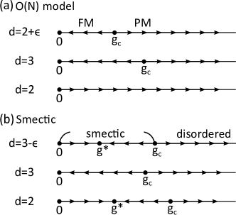
The -model was first studied by Polyakov [6], Nelson and Pelcovits [7] using perturbative renormalization group (RG) in , which shows that for the ferromagnet-paramagnet (FM-PM) transition is described by a critical fixed point at , as illustrated in Fig. 4(a). Consequently, the ordered state is unstable in 2d () at any nonzero temperatures, where the correlation length of the order parameter is finite. This is in contrast to the XY model that has vanished nonlinearity, and at low temperatures exhibits a quasi-long-range ordered Kosterlitz-Thouless phase.
The smectic Goldstone mode theory was studied by Grinstein and Pelcovits [12, 13] using RG for , by Golubović and Wang [57] in , and by Radzihovsky in [30]. Remarkably, for , the smectic ordered state is described by an attractive fixed point at – a stable critical phase [see Fig. 4(b)] 777At the critical dimension , , the smectic is in principle described by a Gaussian fixed point, but with logarithmic corrections to the correlation functions and physical observables due to marginally irrelevant flows [12, 13] akin to the Ising model at .. However, we note that these analyses all consider pure elastic models that neglect topological defects – dislocations in the layered structure, which undoubtedly unbind in 2d at any nonzero temperatures [59]. Thus, these critical phase correlations only extend out to lengths corresponding to distance between topological defects, beyond which the state crosses over to a translationally disordered nematic.
Now we consider the coupling between the two sectors. For the collinear state, the leading order couplings in (88) in angular representation are given by
| (109) |
At , the only marginal correction to the elastic moduli is and the remaining are irrelevant. Therefore, all coupling terms are irrelevant and at low energies the two sectors are decoupled, described by the RG flows in Fig. 4, all of which are asymptotically identical to those in Refs. [12, 13, 30]. Similar argument applies to the coplanar state. However, as discussed in Eq. (95), the Goldstone-mode Hamiltonian is distinct from the collinear state by a replacement
| (110) |
As a result, smectic phonon and the spin field are intrinsically-coupled in the low-energy Hamiltonian (II.3.2). This implies that the spin field can acquire universal power-law correction to its elastic moduli, which are distinct from the in collinear state. We leave the resulting RG analysis to future studies.
III.3 Two-point correlation function of Goldstone modes
Next we calculate the two-point correlation functions of the Goldstone modes. This not only provides spatially resolved properties of the system but also serves as the first step towards a calculation of the structure factor of the following subsection. We note that as discussed above, in principle all Goldstone modes are coupled. However, because they are subdominant, below we neglect the coupling between the smectic () and magnetic ( and ) sectors, a valid approximation at low energies.
III.3.1 Smectic Goldstone mode
Both the collinear and coplanar states are characterized by a smectic phonon, whose correlation function is given by the following logarithmic Caill form [56]:
| (113) |
that exhibits an anisotropic correlation at long scales, with the coefficients in front of the functions differing by a factor two in the perpendicular and parallel directions. In the above, is the exponential-integral function. is the penetration length that characterizes the anisotropy of the smectic state.
In the presence of weak lattice anisotropy, where the spatial rotational symmetry is explicitly broken, the smectic mode is perturbed by a stabilizing modulus, , with the Hamiltonian given by (III.1.4). This deforms the correlation function to be of the following form,
| (114) |
As illustrated in Fig. 5, this introduces a crossover scale , in 3d separating the logarithmic (, ) and long-range-ordered (, ) regimes.

III.3.2 Spin Goldstone modes
For the spin sector, the Goldstone modes at low energies are described by the XY model form, with their correlation function given by
| (115) |
where
| (116) |
The correlator consists of constant and power-law parts, that, as discussed below gives rise to two power-law contributions to the peaks of the static structure factor.
As discussed in Sec. III.1.4, in the presence of SOC that locks the spins perpendicular to , the magnetic Goldstone modes can be pinned with a gap , leading to
| (117) |
where the gap introduces crossover length scales for the parallel/perpendicular directions, beyond which the spin fluctuations are suppressed.
III.4 Structure factor
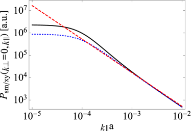
The static spin structure factor is an important experimental characterization of magnetic ordering. Theoretically, this is proportional to equal-time spin-spin correlation function,
| (118) |
where is the volume of the system. Below, we calculate the structure factor for the soft spin-density waves using the Gaussian theory (96), focusing on its asymptotic long-wavelength behaviors and the effects of symmetry-breaking perturbations that are relevant in real materials. As detailed in Appendix D, at the Gaussian level, the asymptotic behavior of the structure factor for the collinear and coplanar states takes the same form:
| (119) |
with
| (120) |
where we retained only the fundamental quasi-Bragg peaks, with real spin-smectic also displaying higher harmonics (). The matrix above is the magnetic sector correlators defined and calculated in Appendix D, with the trace given by
| (123) |
The key characteristic feature of is the 3d quasi-Bragg peak around the ordering wavevector . In the above, is the contributions from short-range correlations that depends smoothly on , is the leading-order singular part due to the quasi-long-range correlation of the smectic phonon, given by ()
| (126) |
with the Debye–Waller factor, and is sub-leading singular contribution coming from the power-law dependence in , (123), which (together with the smectic correlation) is given by
| (129) |
where for simplicity we chose and the nonuniversal temperature-dependent exponent is given by,
| (130) |
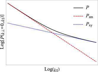
As illustrated in Fig. 6, the structure factor exhibits anisotropic “double-power-law” peaks at with exponents and perpendicular and parallel to the ordering wavevector , respectively. Away from the peaks these crossover to and , as dominated by the sub-leading (but broader) contributions of . The magnitudes of the power-law functions and are nonuniversal, depending on the detailed Goldstone mode dispersions and temperature. In real systems, it may be hard to distinguish the power-law tail of from the nonuniversal contribution . However, the former may still manifest at high temperatures or small stiffness [see Eq. (129)], not only due to the enhanced magnitude of , but also the suppression of by the Debye-Waller factor.
In real crystalline materials, the spin-density waves generally consist of higher harmonics that will also give rise to double-power-law peaks at with modified exponents , see Eq. (6) and Fig. 2. Furthermore, the spin-density waves tend to form domains with their wavevectors pinned by the underlying lattice. In this case, the structure factor is given by the average of those domain contributions, leading to peaks located on the high symmetry axes of the Brillouin zone. As illustrated in Fig. 7, this also leads to finite-size effects that broaden the power-law contributions and , with the leading singular part by widths and ( the averaged domain size, the longest UV scale, within which the smectic dispersion starts to deviate) in the parallel and perpendicular directions, respectively.
As shown in Eq. (III.3.2), the SOC also gives rise to similar effects on by introducing a gap in the magnetic Goldstone-mode correlators, that terminates the power-law dependence around . For the cases that spins are locked perpendicular to the , the collinear and coplanar states have one and two magnetic Goldstone modes gapped, respectively. Accordingly, for the collinear state the asymptotic behaviors of remains the same, while for the coplanar state is broadened by the infrared cutoff introduced by the gap.
In the presence of lattice anisotropy that pins the direction of , the smectic correlator becomes long-range-ordered, see Fig. 5. This sharpens the power-law quasi-Bragg peak of to a delta function Bragg peak, while modifies the exponents of to be . As illustrated in Fig. 7, together with the finite-size effects, this leads to an enhanced peak strength, within the crossover momentum scale (see the black-solid and blue-dotted curves).
Finally, we expect that near a thermal phase transition, the ratio of the spin stiffness to be small, which can lead to a sizable non-singular contribution due to strong spin-sector fluctuations, that depend on the “sub-leading” moduli in (III.1.3) and (III.1.3) for the collinear and coplanar states, respectively. For the coplanar states, there are strong fluctuations on the spiral surface, which may lead to anisotropic arc-shaped peaks, observed in a classical Heisenberg model in Ref. [60].
IV Ginzburg-Landau model
In Sec. II we constructed the spin-density functional designed to give condensation into a spin-smectic state. However, such functional is unable to capture the nature of a continuous phase transition as its disordered state is an isotropic structureless fluid. Here, we instead construct a generalized Ginzburg-Landau ( generalization of de Gennes’ scalar model for conventional smectic liquid crystal [11]) model that gives the smectic as its ordered state and has an additional virtue of describing the continuous transition from the orientationally ordered to the smectic ordered states.
To this end, we propose the following free energy density that incorporates the orientation order that is characterized by the wavevector
| (131) |
In the above,
| (132) |
are the orientational Goldstone mode fluctuations characterizing the “nematic” phase from which the spin-smectic emerges. As for conventional nematics, they are characterized by the standard Frank-Oseen free energy with the splay (), twist () and bend () elastic moduli. The complex vector field, , is the slowly-varying order parameter of spin-smectic in (II) that characterizes the strength of spin order (note that are not unit vectors, with their amplitude growing in the usual Landau way below the transition). As spin-smectic emerges from an anisotropic, orientationally-ordered nematic state. the stiffness of the order parameter are anisotropic, .
For clarity of presentation, in the following discussion we set , with the model then simplifying to
| (133) |
which resembles the Ginzburg-Landau model of a normal-superconductor transition with a nonzero spin-angular momentum pairing (e.g., He3), but with an additional gauge-invariance breaking splay stiffness replacing the Maxwell term for the vector potential.
At high temperatures, , the complex vector field is translationally disordered, leaving the Frank-Oseen free energy that describes the nematic-like unidirectional order of the parent liquid state.
At low temperatures, (and ), the spin-smectic order emerges, characterized by a nonzero order parameter,
| (134) |
where for or , the collinear state that satisfies (18) is energetically preferred with
| (135) |
Instead, for and , the coplanar state that satisfies (22) is more stable with
| (136) |
The state is characterized by the coherence length,
| (137) |
which governs the spatial distortions of of the amplitude and thereby the size of the so-called cybotactic clusters near the critical point, and by the orientational “penetration” length
| (138) |
which is the scale that twist and bend deformation can penetrate through the soft spin-density wave.
Below, we show that at low temperatures this generalized spin-de Gennes model reproduces all the properties of the collinear and coplanar spin-smectic states, but in addition captures the critical properties of the phase transition, whose beyond-mean-field treatment of critical behavior is a challenging problem that we leave to future studies.
IV.1 Collinear state
For the collinear state (135), the coupling terms in (IV) become ()
| (139) |
where we suspended Einstein’s summation convention (no summation over ) and at low temperatures, deep in the collinear spin-smectic state, the minimization of the second term above gives 888This can be done exactly using a Lagrangian multiplier to impose the constraint . See, e.g., Ref. [24]., ):
| (140) |
This leads to the following low-energy Goldstone theory that describes the collinear state
| (141) |
in agreement with our earlier analysis in (II.4) with the identification of the coefficients
| (142) |
which suggests a divergent anisotropy near the critical point, where . As before, deep in the phase, here we also neglected the dislocation defects, i.e., .
IV.2 Coplanar state
For the coplanar spin-smectic state (136), the coupling terms in (IV) reduce to
| (143) |
where we suspended Einstein’s summation convention and in the last line we expressed the out-of-plane fluctuations in terms of using (II.3.3).
In the ordered state, the minimization of the second term above gives an emergent Higgs-like mechanism locking orientational and smectic orders according to
| (144) |
where the dimensionless field . This then gives the Goldstone mode Hamiltonian for the coplanar state
| (145) |
which reduces to (II.3.3) in the absence of dislocations, , with
| (146) |
This again leads to a divergent anisotropy near the critical point, where .
As noted above, in addition to reproducing the corresponding spin-smectic states, the spin-de Gennes model faithfully captures the spin-Nematic-Smectic phase transition that we expect to display rich universal critical phenomenology [62], whose study we leave for the future.
V Quantum dynamics
So far, all of our analysis has been confined to a classical treatment of the spin-smectic states, valid at high temperatures. However, at low temperatures quantum dynamics becomes important, and we need to generalize our model by extending it to include dynamics and quantize it via, e.g., a coherent spin path-integral formulation, following the standard derivation of the conventional antiferromagnetic -model with linear dispersion [9, 10].
To this end, to capture the zero-temperature dynamics and the associated quantum fluctuations, we now introduce the spin Berry phase that is the Wess-Zumino-Witten action that encodes the () spin commutator algebra into the action, corresponding to spin precession generic to all underdamped spin systems.
To extend this to an array of spins, we sum over lattice sites with the action then given by ():
| (147) |
where is the spin magnitude quantum number, is the coherent spin label corresponding to orientation of a spins at , and auxiliary time-like variable was introduced to be able to express covariently in terms of , rather than in terms of its polar () and azimuthal () angles. It is easy to see that is a boundary term that after integral gives the solid angle in (V), swept out by , which quantizes spin in integer multiples of . This also gives the identification of with the physical spin according to and , with the latter an arbitrary reference spin orientation.
Below, we focus on the coplanar state, expressing in terms of the zero-wavevector (uniform, ferromagnetic part, not to be confused with the magnitude of spin in previous sections) and the nonzero wavevector (spiral part) contributions,
| (148) |
where
| (149) |
and the denominator is a normalization factor that ensures . The uniform component must be included despite being gapped in the spin-spiral state, as it encodes the conserved magnetization and has a nontrivial commutation relation with .
We consider small ferromagnetic fluctuations such that
| (150) |
where is the components of perpendicular to , i.e., . Furthermore, because the ground state is not a ferromagnet, uniform magnetization fluctuations are gapped, i.e., characterized by a Hamiltonian
| (151) |
where is the uniform ferromagnetic susceptibility in the coplanar state.
With this the evolution operator is given by ()
| (152) |
where is given by (68). Inserting the form (150) inside and keeping only linear terms in the gapped uniform magnetization , we find
| (153) |
where we dropped the term proportional to , that vanishes (for smooth configurations of ) because it oscillates strongly at wavevector 999This can however lead to nontrivial topological contributions that, e.g., for leads to the distinction between integer and half-integer spins in Heisenberg antiferromagnets [8]. The first term above vanishes because it involves three vectors lying in a plane normal to . With integration by parts, reduces to a total derivative,
| (154) |
where in the last line we dropped the oscillating terms. Integrating over the gapped magnetization field and substituting , we find
| (155) |
where . This form is straightforwardly generalized to spin components, and using the identity (II.3.3), gives
| (156) |
where is defined in (58).
VI Summary and Conclusion
Motivated by a large number of physical realizations of unidirectional orders in liquid crystals, degenerate atomic gases, electronic and in particular frustrated magnetic systems, here we developed a low-energy theory of Goldstone modes, i.e., spin-smectic -model that describes unidirectional “density” waves of generalized -component smectic. We predicted two phases – coplanar and collinear spin-smectics that spontaneously break -spin and -spatial rotational symmetries in addition to the translational symmetry along 101010Strictly speaking, the coplanar smectic state does not break translational symmetry. Instead it breaks tensor product of translations along and rotations around the ordering wavevector down to their diagonal subgroup, namely, ..
Having established two corresponding smectic -models, we focused on the new physical interesting case of and examined spin-smectics’ stability to thermal fluctuations within a harmonic approximation. We showed that these states are characterized by a critical dimensions below which the corresponding mean-field order is unstable, to a state with strongly fluctuating Goldstone modes in . We briefly discussed the nonlinearities that couple the smectic and magnetic sectors, reserving their detailed analysis to a future study.
We then used the developed -models to characterize spin-smectic phases by the correlation functions of their Goldstone modes. In addition to asymptotic behavior the idealized system, we also discussed the effects of weak symmetry-breaking perturbations that exist in real materials: (i) Lattice anisotropy breaking spatial- rotational symmetry by pinning along high symmetry axes of the underlying lattice, that leads to a smectic to XY model crossover for the smectic phonon mode. (ii) Spin-orbit interaction locking the spin orientation to and thereby breaking the rotational symmetries down to their diagonal subgroup. In particular, for the coplanar state, the spin-plane normal vector is frozen along , which gaps out the two magnetic Goldstone modes, akin to cholesterics and DM-interacting helical magnets. In materials with weak DM spin-orbit interactions and weak lattice pinning anisotropy compared to the Heisenberg exchange interactions, we predict that spin-smectic -models will control the low-temperature Goldstone modes and therefore will exhibit spin-smectic structure function over a large intermediate range of length scales before asymptotically crossing over to a conventional -model behavior.
Utilizing these Goldstone modes correlation functions, we computed the static spin structure factors, focusing on their asymptotic long-wavelength behaviors. We showed that at the harmonic level the collinear and coplanar spin-smectics are characterized by the same asymptotic form. In 3d they both exhibit double-power-law quasi-Bragg peaks (in contrast to the usual single-power-law for scalar smectics and delta-function Bragg peaks in conventional magnets) at due to the combined effects of the smectic- and XY- spin Goldstone mode fluctuations. In addition, we discussed specific applications to magnetic systems, including the effects of various symmetry-breaking perturbations and powder averaging over different spin-smectic domains, that change the asymptotic behaviors of the peaks. However, we expect that even in the ideal case without such perturbations, the double-power-law characteristic feature may be weak, and difficult to distinguish from the non-singular short-range correlations. Yet, we found that these novel features are enhanced near a phase transition into the spin-nematic state, where the effective transverse to spin stiffness vanish parametrically faster than its longitudinal counterpart. We leave the required detailed analysis near the critical point to future studies.
We also complemented our spin-smectic -model development with a generalization of a de Gennes-like model that captures the spin-nematic to spin-smectic (NA) phase transition in terms of a complex -vector order parameter characterizing the spin-smectic state. At the mean-field level it describes the phase transition and reproduces precisely the -models of the planar and collinear smectic states. However, it raises a challenging question of true criticality of this spin-NA transition, that we leave for future investigations.
An extension of our study to a quantum spin-smectics is another interesting and open direction to explore. Here, by appending our classical theory with the WZW action–spin precessional dynamics, we derived the quantum dynamic for the coplanar spin state. At Gaussian level it leads to one smectic-like mode (with linear and quadratic dispersion in the parallel and perpendicular directions, respectively) and conventional spin-density wave-like Goldstone modes with linear dispersion. This allows for the study of the dynamic structure function obtained in neutron scattering, with the analysis left for a future study. Our analysis assumes smooth configurations of spins, and thus neglects possible topological terms that could play a nontrivial role in the properties of spin-smectics. We also leave more detailed studies of this to future research.
Our study is based on a symmetric field theory, with the discussion of symmetry-breaking effects incorporated phenomenologically. A more microscopic analysis, that allows a quantitative assessment of such symmetry breaking terms is a necessary next step to assess smectic -model applicability and range of validity in real materials.
Other future directions include but not limited to large- and RG analyses of the smectic -model, the effects of topological defects, and the generalization of spin-smectic states to different representations of the group and to other symmetry groups. We hope our study can stimulate future theoretical and experimental studies in such soft spin-density waves and their generalizations.
Acknowledgement
LR thanks John Toner and Arun Paramekanti for enlightening discussions. This research was supported by the Simons Investigator Award to LR from the Simons Foundation. LR thanks The Kavli Institute for Theoretical Physics for hospitality while this manuscript was in preparation, during Quantum Crystals and Quantum Magnetism workshops, supported by the National Science Foundation under Grant No. NSF PHY-1748958 and PHY-2309135.
Appendix A Analysis of the gradient terms in the smectic model
Here, we evaluate all the symmetry-allowed gradient terms in the field theory (II) up to quartic order in . As discussed in Sec. II, this then leads to universal, low-energy Goldstone mode models for both the collinear and coplanar spin-density wave states. Specifically, we will consider the following quadratic
| (157) |
and quartic terms
| (158) |
We note that the important term in (II) is the linear combinations of the terms above, given by
| (159) |
A.1 collinear state
For the collinear state (80) we find (),
| (160) |
After dropping the oscillating (in space) contributions (that vanish upon spatial integration) the quadratic terms are given by
| (161) |
where we used . The quartic terms are given by
| (162) |
We used above expression in the main text to derive the collinear smectic -model.
A.2 coplanar state
In the coplanar spin-wave state, characterized by the order parameter (49) we instead find
| (163) |
where with . After dropping the oscillating (in space) terms, the quadratic terms are given by
| (164) |
where we used the identity . The quartic terms are given by
| (165) |
and because for the coplanar state.
In terms of and the expressions reduce to
| (166) |
Appendix B Gauge field representation of coplanar -model
In this appendix we reformulate the coplanar smectic -model in terms of gauge (spin-connection) fields constructed from , . For , , (or equivalently , ) and span the spin space:
| (167) |
With this identity, all the terms above can be written in terms of a real vector (in space) field and a complex vector field , defined by
| (168) |
giving
| (169) |
where we used
| (170) |
We use this description to formulate the coplanar spin-smectic -model.
Appendix C Complementary description of smectic model and the term
A complementary description of the spin-smectic was proposed by John Toner, by starting with
| (171) |
where the nematic-like field ensures underlying rotational symmetry. Using this model to derive Goldstone mode theory for the coplanar state (49), at harmonic level in the small expansion of the orthonormal triad in terms of three angles
| (172) | |||||
| (173) |
one obtains
| (174) |
That is, the smectic phonon (spiral phase angle ) is indeed smectic-like, but the two out-of-plane fluctuations of the triad are XY-like. This form does not exhibit the out-of-plane instability of the “soft” sigma model (53).
This suggests that the first derivation is from a non-generic model and therefore misses some important couplings that will appear in a more general model. Examination of the model proposed by Toner shows that it contains a new quartic term, that when averaged over gives
| (175) |
where we used isotropy of the probability distribution. The second term is the stabilizing quartic term that enters crucially for the nonlinear planar spin-smectic -model.
Appendix D Calculation details of the spin-smectic structure factor
In this appendix, we calculate the spin-smectic structure factor in a Gaussian approximation using the angular representation of the spin-density waves in Sec. III.1. We note that the analysis below neglects effects of nonlinearities that may lead to a crossover to a nontrivial spin-smectic fixed point, thereby modifying these predictions at long scales. We first calculate thermal averages of the Goldstone modes, (or superposition of them):
| (176) |
Accordingly the following two-point correlators are given by
| (177) |
where
| (178) |
In general, all Goldstone modes are coupled and therefore for any and . Below, we neglect the coupling between , , and , a valid approximation at low energies. Specifically, we consider the correlators
| (179) |
neglecting all others. The structure factor is given by the Fourier transform of the spin-spin correlation function, (118).
D.1 Collinear state
For the collinear state (80), the spin-spin correlation function in momentum space is given by
| (180) |
where in the second line above we dropped the term proportional to that will average to zero for and then renamed . In the above, is defined in (III.3.1) and , where by using (90) the matrix elements are given by
| (181) |
and all others vanish. Keeping terms up to quadratic order in Goldstone modes, we have
| (185) |
This harmonic approximation is consistent with the one we made on the Hamiltonian and it gives the physically reasonable expression that is symmetric around the axis , i.e., . Within this Gaussian approximation the structure factor is then given by
| (186) |
where and are defined in (III.3.2) and in the last line we rewrote small Goldstone mode fluctuations in an exponential form, .
D.2 Coplanar state
Repeating above analysis and approximations for the coplanar state (49), the spin-spin correlation function in momentum space is then given by
| (187) |
where and H.c. denotes the Hermitian conjugate. Using (III.1.2), the matrix elements are given by
| (188) |
with all others contributions vanishing. For small Goldstone mode fluctuations, we obtain a physically reasonable expression that is symmetric around the axis,
| (192) |
With these approximations the structure factor is then given by
| (193) |
where in the last line we rewrote the small Goldstone mode fluctuations as exponential form, .
The expressions for the collinear (D.1) and coplanar (D.2) structure factors, together with the Goldstone mode correlators (III.3.1) and (III.3.2), lead to the same asymptotic form (III.4), characterized by the following double-power-law peaks
| (194) |
In the above, the leading power-law contribution is from the smectic Goldstone mode fluctuations, given by
| (197) | ||||
| (200) |
where is the Debye-Waller factor, the temperature dependent exponent is given by (130), and we used the change of variable to get the last line. On the other hand, the sub-leading power-law contribution is a consequence of the combined effects of the smectic and XY Goldstone mode fluctuations, given by
| (203) | ||||
| (206) |
where for simplicity we chose and we used the change of variable to get the last line.
References
- Note [1] Throughout the manuscript we will use the term “density” to also refer to spin, Cooper pair, and other generalized densities that transform nontrivially under internal symmetry.
- Chakravarty et al. [1989] S. Chakravarty, B. I. Halperin, and D. R. Nelson, Two-dimensional quantum Heisenberg antiferromagnet at low temperatures, Physical Review B 39, 2344 (1989).
- Lee and Rice [1979] P. A. Lee and T. M. Rice, Electric field depinning of charge density waves, Physical Review B 19, 3970 (1979).
- Wigner [1934] E. Wigner, On the Interaction of Electrons in Metals, Physical Review 46, 1002 (1934).
- Agterberg et al. [2020] D. F. Agterberg, J. S. Davis, S. D. Edkins, E. Fradkin, D. J. Van Harlingen, S. A. Kivelson, P. A. Lee, L. Radzihovsky, J. M. Tranquada, and Y. Wang, The Physics of Pair-Density Waves: Cuprate Superconductors and Beyond, Annual Review of Condensed Matter Physics 11, 231 (2020).
- Polyakov [1975] A. M. Polyakov, Interaction of goldstone particles in two dimensions. Applications to ferromagnets and massive Yang-Mills fields, Physics Letters B 59, 79 (1975).
- Nelson and Pelcovits [1977] D. R. Nelson and R. A. Pelcovits, Momentum-shell recursion relations, anisotropic spins, and liquid crystals in dimensions, Physical Review B 16, 2191 (1977).
- Haldane [1983] F. D. M. Haldane, Nonlinear field theory of large-spin heisenberg antiferromagnets: Semiclassically quantized solitons of the one-dimensional easy-axis Néel state, Physical Review Letters 50, 1153 (1983).
- Haldane [1988] F. D. M. Haldane, O(3) nonlinear model and the topological distinction between integer- and half-integer-spin antiferromagnets in two dimensions, Physical Review Letters 61, 1029 (1988).
- Dombre and Read [1989] T. Dombre and N. Read, Nonlinear models for triangular quantum antiferromagnets, Physical Review B 39, 6797 (1989).
- de Gennes and Prost [1995] P. G. de Gennes and J. Prost, The Physics of Liquid Crystals, 2nd ed. (Clarendon Press, Oxford, 1995).
- Grinstein and Pelcovits [1981] G. Grinstein and R. A. Pelcovits, Anharmonic Effects in Bulk Smectic Liquid Crystals and Other ”One-Dimensional Solids”, Physical Review Letters 47, 856 (1981).
- Grinstein and Pelcovits [1982] G. Grinstein and R. A. Pelcovits, Nonlinear elastic theory of smectic liquid crystals, Physical Review A 26, 915 (1982).
- Radzihovsky and Toner [1997] L. Radzihovsky and J. Toner, Nematic–to–smectic-A transition in aerogel, Physical Review Letters 79, 4214 (1997).
- Radzihovsky and Toner [1999] L. Radzihovsky and J. Toner, Smectic liquid crystals in random environments, Physical Review B 60, 206 (1999).
- Bellini et al. [2001] T. Bellini, L. Radzihovsky, J. Toner, and N. A. Clark, Universality and scaling in the disordering of a smectic liquid crystal, Science 294, 1074 (2001).
- Radzihovsky [2023] L. Radzihovsky, Critical Matter, arXiv e-prints , arXiv:2306.03142 (2023), arXiv:2306.03142 [cond-mat.stat-mech] .
- Lilly et al. [1999] M. P. Lilly, K. B. Cooper, J. P. Eisenstein, L. N. Pfeiffer, and K. W. West, Evidence for an Anisotropic State of Two-Dimensional Electrons in High Landau Levels, Physical Review Letters 82, 394 (1999).
- Koulakov et al. [1996] A. A. Koulakov, M. M. Fogler, and B. I. Shklovskii, Charge Density Wave in Two-Dimensional Electron Liquid in Weak Magnetic Field, Physical Review Letters 76, 499 (1996).
- Moessner and Chalker [1996] R. Moessner and J. T. Chalker, Exact results for interacting electrons in high Landau levels, Physical Review B 54, 5006 (1996).
- Fradkin and Kivelson [1999] E. Fradkin and S. A. Kivelson, Liquid-crystal phases of quantum Hall systems, Physical Review B 59, 8065 (1999).
- MacDonald and Fisher [2000] A. H. MacDonald and M. P. A. Fisher, Quantum theory of quantum Hall smectics, Physical Review B 61, 5724 (2000).
- Radzihovsky and Dorsey [2002] L. Radzihovsky and A. T. Dorsey, Theory of Quantum Hall Nematics, Physical Review Letters 88, 216802 (2002).
- Radzihovsky and Lubensky [2011] L. Radzihovsky and T. C. Lubensky, Nonlinear smectic elasticity of helical state in cholesteric liquid crystals and helimagnets, Physical Review E 83, 051701 (2011).
- Zhai [2015] H. Zhai, Degenerate quantum gases with spin–orbit coupling: A review, Reports on Progress in Physics 78, 026001 (2015).
- Tanzi et al. [2019] L. Tanzi, S. M. Roccuzzo, E. Lucioni, F. Famà, A. Fioretti, C. Gabbanini, G. Modugno, A. Recati, and S. Stringari, Supersolid symmetry breaking from compressional oscillations in a dipolar quantum gas, Nature 574, 382 (2019).
- Fulde and Ferrell [1964] P. Fulde and R. A. Ferrell, Superconductivity in a Strong Spin-Exchange Field, Physical Review 135, A550 (1964).
- Larkin and Ovchinnikov [1964] A. I. Larkin and Y. N. Ovchinnikov, Nonuniform state of superconductors, Zh. Eksp. Teor. Fiz. 47, 1136 (1964).
- Radzihovsky and Vishwanath [2009] L. Radzihovsky and A. Vishwanath, Quantum Liquid Crystals in an Imbalanced Fermi Gas: Fluctuations and Fractional Vortices in Larkin-Ovchinnikov States, Physical Review Letters 103, 010404 (2009).
- Radzihovsky [2011] L. Radzihovsky, Fluctuations and phase transitions in Larkin-Ovchinnikov liquid-crystal states of a population-imbalanced resonant Fermi gas, Physical Review A 84, 023611 (2011).
- Radzihovsky and Choi [2009] L. Radzihovsky and S. Choi, -Wave Resonant Bose Gas: A Finite-Momentum Spinor Superfluid, Physical Review Letters 103, 095302 (2009).
- Choi and Radzihovsky [2011] S. Choi and L. Radzihovsky, Finite-momentum superfluidity and phase transitions in a -wave resonant Bose gas, Physical Review A 84, 043612 (2011).
- Hsieh et al. [2022] T.-C. Hsieh, H. Ma, and L. Radzihovsky, Helical superfluid in a frustrated honeycomb Bose-Hubbard model, Physical Review A 106, 023321 (2022).
- Note [2] These are distinct from another interesting class of helimagnets arising from the chiral Dzyaloshinskii-Moriya (DM) spin-orbit interaction that drives the helical structure. Such DM helical states are less symmetrical than those considered in this paper, and do not exhibit independent and symmetries. In such systems, equivalent to a cholesteric liquid crystal the orientations of and are locked, and thus at low energies its Goldstone mode reduces to that of a smectic, as discussed in Ref. [24]. Physical realizations of such system include MnSi, which is an itinerant ferromagnet exhibiting helical structure at low temperatures. These systems show anomalous magnetic [50, 51, 52] and transport [53] behavior as probed over different temperature, pressure, and magnetic field.
- Bergman et al. [2007] D. Bergman, J. Alicea, E. Gull, S. Trebst, and L. Balents, Order-by-disorder and spiral spin-liquid in frustrated diamond-lattice antiferromagnets, Nature Physics 3, 487 (2007).
- Mulder et al. [2010] A. Mulder, R. Ganesh, L. Capriotti, and A. Paramekanti, Spiral order by disorder and lattice nematic order in a frustrated Heisenberg antiferromagnet on the honeycomb lattice, Physical Review B 81, 214419 (2010).
- Tristan et al. [2005] N. Tristan, J. Hemberger, A. Krimmel, H.-A. Krug von Nidda, V. Tsurkan, and A. Loidl, Geometric frustration in the cubic spinels (, , and ), Physical Review B 72, 174404 (2005).
- Suzuki et al. [2007] T. Suzuki, H. Nagai, M. Nohara, and H. Takagi, Melting of antiferromagnetic ordering in spinel oxide CoAl2O4, Journal of Physics: Condensed Matter 19, 145265 (2007).
- Fritsch et al. [2004] V. Fritsch, J. Hemberger, N. Büttgen, E.-W. Scheidt, H.-A. Krug von Nidda, A. Loidl, and V. Tsurkan, Spin and orbital frustration in and , Physical Review Letters 92, 116401 (2004).
- Gao et al. [2022] S. Gao, M. A. McGuire, Y. Liu, D. L. Abernathy, C. dela Cruz, M. Frontzek, M. B. Stone, and A. D. Christianson, Spiral Spin Liquid on a Honeycomb Lattice, Physical Review Letters 128, 227201 (2022).
- Bordelon et al. [2021] M. M. Bordelon, C. Liu, L. Posthuma, E. Kenney, M. J. Graf, N. P. Butch, A. Banerjee, S. Calder, L. Balents, and S. D. Wilson, Frustrated heisenberg model within the stretched diamond lattice of , Physical Review B 103, 014420 (2021).
- Ramirez [1994] A. P. Ramirez, Strongly Geometrically Frustrated Magnets, Annual Review of Materials Research 24, 453 (1994).
- Balents [2010] L. Balents, Spin liquids in frustrated magnets, Nature 464, 199 (2010).
- Villain et al. [1980] J. Villain, R. Bidaux, J.-P. Carton, and R. Conte, Order as an effect of disorder, Journal de Physique 41, 1263 (1980).
- Henley [1989] C. L. Henley, Ordering due to disorder in a frustrated vector antiferromagnet, Physical Review Letters 62, 2056 (1989).
- Note [3] Generally, the wavevector that minimizes the energy , as it can be corrected by other (than ) gradient terms and higher-order fluctuations.
- Note [4] We do not consider mutli-, nor non-Landau spin liquid states [43]. Determining the true ground state among the single- and these states is a challenging microscopic question that falls outside of effective field theory approach taken here and is best addressed numerically.
- Note [5] On this account, higher order gradient quartic-in- terms can be included, but add nothing new beyond those already included in (II), which is the minimum form required for a generic description, as we verify a posteriori.
- Note [6] Alternatively, we can consider orthonormal basis vectors of the spin space: , , and (). The generators of rotation that act on the orthonormal diad correspond to the , , and planes. This then leads to Goldstone modes that live on the compact manifold, with and (for a given choice) corresponding to the rotations of and , respectively.
- Pfleiderer et al. [2004] C. Pfleiderer, D. Reznik, L. Pintschovius, H. v Löhneysen, M. Garst, and A. Rosch, Partial order in the non-Fermi-liquid phase of MnSi, Nature 427, 227 (2004).
- Grigoriev et al. [2005] S. V. Grigoriev, S. V. Maleyev, A. I. Okorokov, Yu. O. Chetverikov, R. Georgii, P. Böni, D. Lamago, H. Eckerlebe, and K. Pranzas, Critical fluctuations in MnSi near : A polarized neutron scattering study, Physical Review B 72, 134420 (2005).
- Mühlbauer et al. [2009] S. Mühlbauer, B. Binz, F. Jonietz, C. Pfleiderer, A. Rosch, A. Neubauer, R. Georgii, and P. Böni, Skyrmion Lattice in a Chiral Magnet, Science 323, 915 (2009).
- Neubauer et al. [2009] A. Neubauer, C. Pfleiderer, B. Binz, A. Rosch, R. Ritz, P. G. Niklowitz, and P. Böni, Topological Hall Effect in the Phase of MnSi, Physical Review Letters 102, 186602 (2009).
- Mermin and Wagner [1966] N. D. Mermin and H. Wagner, Absence of ferromagnetism or antiferromagnetism in one- or two-dimensional isotropic heisenberg models, Physical Review Letters 17, 1133 (1966).
- Hohenberg [1967] P. C. Hohenberg, Existence of long-range order in one and two dimensions, Physical Review 158, 383 (1967).
- Caillé [1972] A. Caillé, Remarks on the scattering of X-rays by A-type smectics, C.R. Seances Acad. Sci., Ser. B 274, 891 (1972).
- Golubović and Wang [1992] L. Golubović and Z.-G. Wang, Anharmonic elasticity of smectics A and the Kardar-Parisi-Zhang model, Physical Review Letters 69, 2535 (1992).
- Note [7] At the critical dimension , , the smectic is in principle described by a Gaussian fixed point, but with logarithmic corrections to the correlation functions and physical observables due to marginally irrelevant flows [12, 13] akin to the Ising model at .
- Toner and Nelson [1981] J. Toner and D. R. Nelson, Smectic, cholesteric, and Rayleigh-Benard order in two dimensions, Physical Review B 23, 316 (1981).
- Glittum and Syljuåsen [2021] C. Glittum and O. F. Syljuåsen, Arc-shaped structure factor in the classical heisenberg model on the triangular lattice, Physical Review B 104, 184427 (2021).
- Note [8] This can be done exactly using a Lagrangian multiplier to impose the constraint . See, e.g., Ref. [24].
- Halperin et al. [1974] B. I. Halperin, T. C. Lubensky, and S.-k. Ma, First-order phase transitions in superconductors and smectic- liquid crystals, Phys. Rev. Lett. 32, 292 (1974).
- Note [9] This can however lead to nontrivial topological contributions that, e.g., for leads to the distinction between integer and half-integer spins in Heisenberg antiferromagnets [8].
- Note [10] Strictly speaking, the coplanar smectic state does not break translational symmetry. Instead it breaks tensor product of translations along and rotations around the ordering wavevector down to their diagonal subgroup, namely, .
