LASER: Linear Compression in Wireless Distributed Optimization

Abstract

Data-parallel SGD is the de facto algorithm for distributed optimization, especially for large scale machine learning. Despite its merits, communication bottleneck is one of its persistent issues. Most compression schemes to alleviate this either assume noiseless communication links, or fail to achieve good performance on practical tasks. In this paper, we close this gap and introduce LASER: LineAr CompreSsion in WirEless DistRibuted Optimization. LASER capitalizes on the inherent low-rank structure of gradients and transmits them efficiently over the noisy channels. Whilst enjoying theoretical guarantees similar to those of the classical SGD, LASER shows consistent gains over baselines on a variety of practical benchmarks. In particular, it outperforms the state-of-the-art compression schemes on challenging computer vision and GPT language modeling tasks. On the latter, we obtain $50$-$64\%$ improvement in perplexity over our baselines for noisy channels. Code is available at https://github.com/Bond1995/LASER.

[1]hyperparameters: #1 [1]input: #1 [1]initialization: #1 [1]prerequisites: #1 [1]initialize #1 [1]notation: #1 [1]note: #1 [At]AtEndAt [At]AtEndAt[1]at #1 doend at [For]ForEndFor [For]ForEndFor[1]for #1 doend for [Prerequisites]PrerequisitesEndPrerequisites [Prerequisites]PrerequisitesEndPrerequisites[0]prerequisites

1 Introduction

Distributed optimization is one of the most widely used frameworks for training large scale deep learning models (Bottou et al., 2018; Dean et al., 2012; Tang et al., 2020). In particular, data-parallel SGD is the workhorse algorithm for this task. Underpinning this approach is the communication of large gradient vectors between the workers and the central server which performs their aggregation. While these methods harness the inherent parallelism to reduce the overall training time, their communication cost is a major bottleneck that limits scalability to large models. Design of communication-efficient distributed algorithms is thus a must for reaping the full benefits of distributed optimization (Xu et al., 2020).

Existing approaches to reduce the communication cost can be broadly classified into two themes: (i) compressing the gradients before transmission; or (ii) utilizing the communication link for native ‘over-the-air’ aggregation (averaging) across workers. Along (i), a number of gradient compression schemes have been designed such as quantization (Bernstein et al., 2018; Vargaftik et al., 2022), sparsification (Aji & Heafield, 2017; Isik et al., 2022), hybrid methods (Jiang et al., 2018; Basu et al., 2019), and low-rank compression (Wang et al., 2018; Vogels et al., 2019). These methods show gains over the full-precision SGD in various settings (Xu et al. (2020) is a detailed survey). Notwithstanding the merits, their key shortcoming is that they assume a noiseless communication link between the clients and the server. In settings such as federated learning with differential privacy or wireless communication, these links are noisy. Making them noiseless requires error-correcting codes which exacerbates the latency, as the server needs to wait till it receives the gradient from each worker before aggregating (Guo et al., 2020).

Under theme (ii), communication cost is reduced by harnessing the physical layer aspects of (noisy) communication. In particular, the superposition nature of wireless channels is exploited to perform over-the-air averaging of gradients across workers, which reduces the latency, see e.g. (Shi et al., 2020) and the references therein. Notable works include A-DSGD (Amiri & Gündüz, 2020b), analog-gradient-aggregation (Guo et al., 2020; Zhu et al., 2019), channel aware quantization (Chang & Tandon, 2020), etc. However, to the best of our knowledge, the majority of these approaches are restricted to synthetic datasets and shallow neural networks (often single layer) and do not scale well to the practical neural network models (which we verify in Sec. 4). This leads to a natural question:

Can we design efficient and practical gradient compression schemes for noisy communication channels?

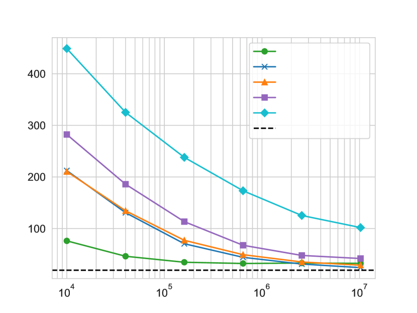
Figure 1: Final test perplexity after 20k iterations (lower is better) vs. power budget for GPT-2 language modeling on WikiText-103. LASER consistently requires orders-of-magnitude less power than other methods for the same perplexity.

Table 1: Power required (lower is better) to reach the target perplexity on WikiText-103. Z-SGD sends the uncompressed gradients directly, while LASER sends a rank-4 approximation. LASER requires $16\times$ less power than Z-SGD to achieve the target perplexity over a wide interval. In the very-high-power regime with perplexity close to that of the noiseless SGD, we see no power gains.

Target	Power required		Reduction
	Z-SGD	LASER
$80$	$160\,\mathrm{K}$	$10\,\mathrm{K}$	$16\times$
$50$	$640\,\mathrm{K}$	$40\,\mathrm{K}$	$16\times$
$40$	$2560\,\mathrm{K}$	$160\,\mathrm{K}$	$16\times$
$35$	$2560\,\mathrm{K}$	$160\,\mathrm{K}$	$16\times$

In this work, we precisely address this and propose LASER, a principled gradient compression scheme for distributed training over wireless noisy channels. Specifically, we make the following contributions:

• Capitalizing on the inherent low-rank structure of the gradients, LASER efficiently computes these low-rank factors and transmits them reliably over the noisy channel while allowing the gradients to be averaged in transit (Sec. 3).

• We show that LASER enjoys similar convergence rate as that of the classical SGD for both quasi-convex and non-convex functions, except for a small additive constant depending on the channel degradation (Thm 1).

• We empirically demonstrate the superiority of LASER over the baselines on the challenging tasks of (i) language modeling with GPT-2 $\rightarrow$ WikiText-103 and (ii) image classification with ResNet18 $\rightarrow$ (Cifar10, Cifar100) and 1-layer NN $\rightarrow$ Mnist. With high gradient compression ($165\times$), LASER achieves $50$-$64\%$ perplexity improvement in the low and moderate power regimes on WikiText-103. To the best of our knowledge, LASER is the first to exhibit such gains for GPT language modeling (Sec. 4).

Notation. Euclidean vectors and matrices are denoted by bold letters $\boldsymbol{x},\boldsymbol{y},\boldsymbol{M}$, etc. $\|\cdot\|$ denotes the Frobenius norm for matrices and the $\ell_{2}$-norm for Euclidean vectors. $\mathcal{O}(\cdot)$ is an upper bound subsuming universal constants whereas $\widetilde{\mathcal{O}}(\cdot)$ hides any logarithmic problem-variable dependencies.

2 Background

Distributed optimization. Consider the (synchronous) data-parallel distributed setting where we minimize an objective $f:\mathbb{R}^{d}\to\mathbb{R}$ defined as the empirical loss on a global dataset $\mathcal{D}=\{(\boldsymbol{x}_{j},y_{j})\}_{j=1}^{N}$:

$$\min_{\boldsymbol{\theta}\in\mathbb{R}^{d}}f(\boldsymbol{\theta}),\quad f(\boldsymbol{\theta})\triangleq\frac{1}{N}\sum_{j=1}^{N}\ell(\boldsymbol{x}_{j},y_{j};\boldsymbol{\theta}),$$

where $\ell(\cdot)$ evaluates the loss for each data sample $(\boldsymbol{x}_{j},y_{j})$ on model $\boldsymbol{\theta}$. In this setup, there are $k$ (data-homogeneous) training clients, where the $i^{\text{th}}$ client has access to a stochastic gradient oracle $\boldsymbol{g}_{i}$, e.g. mini-batch gradient on a set of samples randomly chosen from $\mathcal{D}$, such that $\mathbb{E}[\boldsymbol{g}_{i}|\boldsymbol{\theta}]=\nabla f(\boldsymbol{\theta})$ for all $\boldsymbol{\theta}\in\mathbb{R}^{d}$. In distributed SGD (Robbins & Monro, 1951; Bottou et al., 2018), the server aggregates all $\boldsymbol{g}_{i}$s and performs the following updates:

$$\begin{gathered}\boldsymbol{\theta}_{t+1}=\boldsymbol{\theta}_{t}-\gamma_{t}\cdot\frac{1}{k}\sum_{i=1}^{k}\boldsymbol{g}_{i}^{(t)},\\ \mathbb{E}[\boldsymbol{g}_{i}^{(t)}|\boldsymbol{\theta}_{t}]=\nabla f(\boldsymbol{\theta}_{t}),\quad t\geq 0,\end{gathered}$$ (SGD)

where $\{\gamma_{t}\}_{t\geq 0}$ is a stepsize schedule. Implicit here is the assumption that the communication link between the clients and the server is noiseless, which we expound upon next.

Communication model. For the communication uplink from the clients to the server, we consider the standard wireless channel for over-the-air distributed learning (Amiri & Gündüz, 2020a; Guo et al., 2020; Zhu et al., 2019; Chang & Tandon, 2020; Wei & Shen, 2022a): the additive slow-fading channel, e.g., the classical multiple-access-channel (Nazer & Gastpar, 2007). The defining property of this family is the superposition of incoming wireless signals (enabling over-the-air computation) possibly corrupted together with an independent channel noise (Shi et al., 2020). Specifically, we denote the channel as a (random) mapping $\mathcal{Z}_{P}(\cdot)$ that transforms the set of (time-varying) messages transmitted by the clients $\{\boldsymbol{x}_{i}\}_{i\in[k]}\subset\mathbb{R}^{d}$ to its noisy version $\boldsymbol{y}\in\mathbb{R}^{d}$ received by the server:

$$\begin{split}\boldsymbol{y}&=\mathcal{Z}_{P}(\{\boldsymbol{x}_{i}\})\triangleq\sum_{i=1}^{k}\boldsymbol{x}_{i}+\boldsymbol{Z},\\ &\hskip 50.00008pt\|\boldsymbol{x}_{i}\|^{2}\leq P_{t},~{}\frac{1}{T}\sum_{t=0}^{T-1}P_{t}\leq P,\end{split}$$ (1)

where the noise $\boldsymbol{Z}\in\mathbb{R}^{d}$ is independent of the channel inputs and has zero mean and unit variance per dimension, i.e. $\mathbb{E}\|\boldsymbol{Z}\|^{2}=d$. The power constraint on each client $\|\boldsymbol{x}_{i}\|^{2}\leq P_{t}$ at time $t$ serves as a communication cost (and budget), while the power policy $\{P_{t}\}$ allots the total budget $P$ over $T$ epochs as per the average power constraint (Wei & Shen, 2022b; Amiri & Gündüz, 2020b). A key metric that captures the channel degradation quality is the signal-to-noise ratio per coordinate ($\mathrm{SNR}$), defined as the ratio between the average signal energy ($P$) and that of the noise ($d$), i.e. $\mathrm{SNR}\triangleq P/d$. The larger it is the better the signal fidelity. The power budget $P$ encourages the compression of signals: if each client can transmit the same information $\boldsymbol{x}_{i}$ via fewer entries (smaller $d$), they can utilize more power per entry (higher $\mathrm{SNR}$) and hence a more faithful signal.

The downlink communication from the server to the clients is usually modeled as a standard broadcast channel (Cover, 1972): for input ${\boldsymbol{x}}$ with $\|\boldsymbol{x}\|^{2}\leq P_{b}$, the output $\boldsymbol{y}_{i}=\boldsymbol{x}+\boldsymbol{Z}_{i}$, one for each of the clients. Usually in practice, $P_{b}\gg P$ and therefore we set $P_{b}=\infty$, though our results readily extend to finite $P_{b}$.

In the rest of the paper by channel we mean the uplink channel. The channel model in Eq. (1) readily generalizes to the fast fading setup as discussed in Sec. 4.

Gradient transmission over the channel. In the distributed optimization setting the goal is to communicate the (time-varying) local gradients $\boldsymbol{g}_{i}\in\mathbb{R}^{d}$ to the central server over the noisy channel in Eq. (1). Here we set the messages $\boldsymbol{x}_{i}$ as linear scaling of gradients (as we want to estimate the gradient average), i.e. $\boldsymbol{x}_{i}=a_{i}\,\boldsymbol{g}_{i}$ with the scalars $a_{i}\in\mathbb{R}$ enforcing the power constraints:

$$\boldsymbol{y}=\sum_{i=1}^{k}a_{i}\,\boldsymbol{g}_{i}+\boldsymbol{Z},\quad\|a_{i}\,\boldsymbol{g}_{i}\|^{2}\leq P_{t}.$$ (2)

Now the received signal is a weighted sum of the gradients corrupted by noise, whereas we need the sum of the gradients $\sum_{i}\boldsymbol{g}_{i}$ (upto zero mean additive noise) for the model training. Towards this goal, a common mild technical assumption is that the gradient norms $\{\|\boldsymbol{g}_{i}\|\}$ are known at the receiver at each communication round (Chang & Tandon, 2020; Guo et al., 2020) (can be relaxed in practice, Sec. 4). The optimal scalars are then given by $a_{i}=\sqrt{P_{t}}/(\max_{j}\|\boldsymbol{g}_{j}\|),\forall i\in[K]$, which are uniform across all the clients (§ E.1). Now substituting this $a_{i}$ in Eq. (2) and rearranging, the effective channel can be written as

$$\boldsymbol{y}=\widetilde{\mathcal{Z}}_{P}(\{\boldsymbol{g}_{i}\})\triangleq\frac{1}{k}\sum_{i=1}^{k}\boldsymbol{g}_{i}+\frac{\max_{i}\|\boldsymbol{g}_{i}\|}{k\sqrt{P_{t}}}\,\boldsymbol{Z}.$$ (noisy channel)

Equivalently, we can assume this as the actual channel model where the server receives the gradient average corrupted by a zero mean noise proportional to the gradients. Note that the noise magnitude decays in time as gradients converge to zero. We denote $\widetilde{\mathcal{Z}}_{P}(\cdot)$ as simply $\mathcal{Z}_{P}(\cdot)$ henceforth as these two mappings are equivalent.

Z-SGD. Recall that the SGD aggregates the uncompressed gradients directly. In the presence of the noisy channel, it naturally modifies to

$$\boldsymbol{\theta}_{t+1}=\boldsymbol{\theta}_{t}-\gamma_{t}\,\mathcal{Z}_{P}(\{\boldsymbol{g}_{i}^{(t)}\}).$$ (Z-SGD)

Thus Z-SGD is a canonical baseline to compare against. It has two sources of stochasticity: one stemming for the stochastic gradients and the other from the channel noise. While the gradient in the Z-SGD update still has the same conditional mean as the noiseless case (zero mean Gaussian in noisy channel), it has higher variance due to the Gaussian term. When $P=\infty$, Z-SGD reduces to SGD.

3 LASER: Novel linear compression cum transmission scheme

In this section we describe our main contribution, LASER, a novel method to compress gradients and transmit them efficiently over noisy channels. The central idea underpinning our approach is that, given the channel power constraint in Eq. (1), we can get a more faithful gradient signal at the receiver by transmitting its ‘appropriate’ compressed version (fewer entries sent and hence more power per entry) as opposed to sending the full-gradient naively as in Z-SGD. This raises a natural question: what’s a good compression scheme that facilitates this? To address this, we posit that we can capitalize on the inherent low-rank structure of the gradient matrices (Martin & Mahoney, 2021; Mazumder et al., 2010; Yoshida & Miyato, 2017) for efficient gradient compression and transmission. Indeed, as illustrated below and in Thm 1, we can get a variance reduction of the order of the smaller dimension when the gradient matrices are approximately low-rank.

More concretely, let us consider the single worker case where the goal is to transmit the stochastic gradient $\boldsymbol{g}\in\mathbb{R}^{m\times m}$ (viewed as a matrix) to the server with constant power $P_{t}=P$. Further let’s suppose that $\boldsymbol{g}$ is approximately rank-one, i.e. $\boldsymbol{g}\approx\boldsymbol{p}\boldsymbol{q}^{\top}$, with the factors $\boldsymbol{p},\boldsymbol{q}\in\mathbb{R}^{m}$ known. If we transmit $\boldsymbol{g}$ uncompressed over the noisy channel, as in Z-SGD, the server receives $\boldsymbol{y}_{\textsc{Z-SGD}}=\boldsymbol{g}+(\|\boldsymbol{g}\|/\sqrt{P})~{}\boldsymbol{Z}\in\mathbb{R}^{m\times m}$. On the other hand, if we capitalize on the low-rank structure of $\boldsymbol{g}$ and instead transmit the factors $\boldsymbol{p}$ and $\boldsymbol{q}$ with power $P/2$ each, the server would receive:

$$\begin{gathered}\boldsymbol{y}_{\boldsymbol{p}}=\boldsymbol{p}+(\sqrt{2}\|\boldsymbol{p}\|/\sqrt{P})~{}\boldsymbol{Z}_{\boldsymbol{p}}\in\mathbb{R}^{m},\\ \boldsymbol{y}_{\boldsymbol{q}}=\boldsymbol{q}+(\sqrt{2}\|\boldsymbol{q}\|/\sqrt{P})~{}\boldsymbol{Z}_{\boldsymbol{q}}\in\mathbb{R}^{m},\end{gathered}$$

where $\boldsymbol{Z}_{\boldsymbol{p}}$ and $\boldsymbol{Z}_{\boldsymbol{q}}$ are the channel noise. Now we reconstruct the stochastic gradient as

$$\boldsymbol{y}_{\textsc{LASER}}\triangleq\boldsymbol{y}_{\boldsymbol{p}}\boldsymbol{y}_{\boldsymbol{q}}^{\top}=(\boldsymbol{p}+(\sqrt{2}\|\boldsymbol{p}\|/\sqrt{P})~{}\boldsymbol{Z}_{\boldsymbol{p}})\\ \cdot(\boldsymbol{q}+(\sqrt{2}\|\boldsymbol{q}\|/\sqrt{P})~{}\boldsymbol{Z}_{\boldsymbol{q}})^{\top}.$$ (3)

Conditioned on the gradient $\boldsymbol{g}$, while the received signal $\boldsymbol{y}$ has the same mean $\boldsymbol{g}$ under both Z-SGD and LASER, we observe that for Z-SGD it has variance $\mathbb{E}\|\boldsymbol{y}_{\textsc{Z-SGD}}-\boldsymbol{g}\|^{2}=\|\boldsymbol{g}\|^{2}/\mathrm{SNR}$ with $\mathrm{SNR}\triangleq P/m^{2}$, whereas that of LASER is roughly $\|\boldsymbol{g}\|^{2}\cdot(4/m\mathrm{SNR})(1+1/(m\mathrm{SNR}))$, as further elaborated in Definition 1. When $\mathrm{SNR}$ is of constant order $\Omega(1)$, we observe that the variance for LASER is roughly $\mathcal{O}(m)$ times smaller than that of Z-SGD, which is significant given that variance directly affects the convergence speed of stochastic-gradient based methods (Bottou et al., 2018).

More generally, even if the gradients are not inherently low-rank and we only know their rank factors approximately, with standard techniques like error-feedback (Seide et al., 2014) we can naturally generalize the aforementioned procedure, which is the basis for LASER. Alg. 1 below details LASER and Thm 1 establishes its theoretical justification. While LASER works with any power policy $\{P_{t}\}$ in noisy channel, it suffices to consider the constant law $P_{t}=P$ as justified in Sec. 4.2.

3.1 Algorithm

Algorithm 1 LASER

input: initial model parameters $\boldsymbol{\theta}\in\mathbb{R}^{m\times n}$, learning rate $\gamma$, compression rank $r$, power budget $P$output: trained parameters $\boldsymbol{\theta}$each worker $i=1,\ldots,k$memory $\boldsymbol{e}_{i}\leftarrow\mathbf{0}\in\mathbb{R}^{m\times n}$each iterate $t=0,\ldots$Compute a stochastic gradient $\boldsymbol{g}_{i}\in\mathbb{R}^{m\times n}$$\boldsymbol{M}_{i}$$\leftarrow\boldsymbol{e}_{i}+\gamma\boldsymbol{g}_{i}$$\boldsymbol{P}_{i},\boldsymbol{Q}_{i}$$\leftarrow\mathcal{C}_{r}(\boldsymbol{M}_{i})$$\boldsymbol{e}_{i}$$\leftarrow\boldsymbol{M}_{i}-\textsc{decompress}(\mathcal{C}_{r}(\boldsymbol{M}_{i}))$$\boldsymbol{\alpha},\boldsymbol{\beta}$$\leftarrow\textsc{poweralloc}(\{\mathcal{C}_{r}(\boldsymbol{M}_{j}),\boldsymbol{M}_{j}\})$$\boldsymbol{Y}_{\boldsymbol{p}},~{}\boldsymbol{Y}_{\boldsymbol{q}}$$\leftarrow\mathcal{Z}_{\boldsymbol{\alpha}}(\{\boldsymbol{P}_{j}\}),~{}\mathcal{Z}_{\boldsymbol{\beta}}(\{\boldsymbol{Q}_{j}\})$$\boldsymbol{g}$$\leftarrow\textsc{decompress}(\boldsymbol{Y}_{\boldsymbol{p}},\boldsymbol{Y}_{\boldsymbol{q}})$$\boldsymbol{\theta}$$\leftarrow\boldsymbol{\theta}-\boldsymbol{g}$

For distributed training of neural network models, we apply Alg. 1 to each layer independently. Further we use it only for the weight matrices (fully connected layers) and the convolutional filters (after reshaping the multi-dimensional tensors to matrices), and transmit the bias vectors uncompressed. Now we delineate the two main components of LASER: (i) Gradient compression + Error-feedback (EF), and (ii) Power allocation + Channel transmission.

Gradient compression and error feedback (7-9). Since we transmit low-rank gradient approximations, we use error feedback (EF) to incorporate the previous errors into the current gradient update. This ensures convergence of SGD with biased compressed gradients (Karimireddy et al., 2019). For the rank-$r$ compression of the updated gradient $\boldsymbol{M}$, $\mathcal{C}_{r}(\boldsymbol{M})$, we use the PowerSGD algorithm from Vogels et al. (2019), a linear compression scheme to compute the left and right singular components $\boldsymbol{P}\in\mathbb{R}^{m\times r}$ and $\boldsymbol{Q}\in\mathbb{R}^{n\times r}$ respectively. PowerSGD uses a single step of the subspace iteration (Stewart & Miller, 1975) with a warm start from the previous updates to compute these factors. The approximation error, $\boldsymbol{M}-\boldsymbol{P}\boldsymbol{Q}^{\top}$, is then used to update the error-feedback for next iteration. Note that the clients do not have access to the channel output and only include the local compression errors into their feedback. The decompression function in line $9$ is given by $\textsc{decompress}(\boldsymbol{P},\boldsymbol{Q})\triangleq\boldsymbol{P}\boldsymbol{Q}^{\top}\in\mathbb{R}^{m\times n}$.

Power allocation and channel transmission (10-11). This block is similar to Eq. (3) we saw earlier but generalized to multiple workers and higher rank. For each client, to transmit the rank-$r$ factors $\boldsymbol{P}$ and $\boldsymbol{Q}$ over the noisy channel, we compute the corresponding power-allocation vectors $\boldsymbol{\alpha},\boldsymbol{\beta}\in\mathbb{R}_{+}^{r}$, given by $\boldsymbol{\alpha},\boldsymbol{\beta}=\textsc{poweralloc}(\boldsymbol{P},\boldsymbol{Q},\boldsymbol{M})$. This allocation is uniform across all the clients. Given these power scalars, all the clients synchronously transmit the corresponding left factors over the channel which results in $\boldsymbol{Y}_{\boldsymbol{p}}\in\mathbb{R}^{m\times r}$. Similarly for $\boldsymbol{Y}_{\boldsymbol{q}}\in\mathbb{R}^{n\times r}$. Finally, the stochastic gradient for the model update is reconstructed as $\boldsymbol{g}=\boldsymbol{Y}_{\boldsymbol{p}}\boldsymbol{Y}_{\boldsymbol{q}}^{\top}$. For brevity we defer the full details to § E.1.

3.2 Theoretical results

We now provide theoretical justification for LASER for learning parameters in $\mathbb{R}^{m\times n}$ with $m\leq n$ (without loss of generality). While our algorithm works for any number of clients, for the theory we consider $k=1$ to illustrate the primary gains with our approach. Our results readily extend to the multiple clients setting following Cordonnier (2018). Specifically, Thm 1 below highlights that the asymptotic convergence rate of LASER is almost the same as that of the classical SGD, except for a small additive constant $\lambda_{\textsc{LASER}}$ which is $\mathcal{O}(m)$ times smaller than that of Z-SGD. Our results hold for both quasi-convex and arbitrary non-convex functions. We start with the preliminaries.

Definition 1 (Channel influence factor).

For any compression cum transmission algorithm $\mathrm{ALG}$, let $\boldsymbol{y}_{\mathrm{ALG}}(\boldsymbol{g})$ be the reconstructed gradient at the server after transmitting $\boldsymbol{g}$ over the noisy channel. Then the channel influence factor $\lambda_{\mathrm{ALG}}$ is defined as

$$\lambda_{\mathrm{ALG}}\triangleq\frac{\mathbb{E}_{\boldsymbol{Z}}\|\boldsymbol{y}_{\mathrm{ALG}}(\boldsymbol{g})-\boldsymbol{g}\|^{2}}{\|\boldsymbol{g}\|^{2}}.$$ (4)

The influence factor gauges the effect of the channel on the variance of the final gradient $\boldsymbol{y}_{\mathrm{ALG}}$: if the original stochastic gradient $\boldsymbol{g}$ has variance $\sigma^{2}$ with respect to the actual gradient $\nabla f$, then $\boldsymbol{y}_{\mathrm{ALG}}$ has $(1+\lambda_{\mathrm{ALG}})\sigma^{2}$. Note that this variance directly affects the convergence speed of the SGD and hence the smaller $\lambda_{\mathrm{ALG}}$ is, the better the compression scheme is. In view of this, the following fact (§ B.2) illustrates the crucial gains of LASER compared to Z-SGD, which are roughly of order $\mathcal{O}(m)$:

$$\lambda_{\textsc{LASER}} \leq\frac{4}{(m/r)\mathrm{SNR}}\left(1+\frac{1}{(n/r)\mathrm{SNR}}\right)$$

$$\ll\frac{1}{\mathrm{SNR}}=\lambda_{\textsc{Z-SGD}}.$$ (5)

In the low-rank (Vogels et al., 2019) and constant-order SNR regime where $r=\mathcal{O}(1)$ and $\mathrm{SNR}=\Omega(1)$, we observe that $\lambda_{\textsc{LASER}}$ is roughly $\mathcal{O}(m)$ times smaller than $\lambda_{\textsc{Z-SGD}}$. In other words, the effective $\mathrm{SNR}$ seen by LASER roughly gets boosted to $\mathcal{O}(m\,\mathrm{SNR})$ due to capitalizing on the low-rank factors whereas Z-SGD perceives only the standard factor $\mathrm{SNR}$. Constant-order SNR, i.e. $P/mn=\Omega(1)$, means that the energy used to transmit each coordinate is roughly a constant, analogous to the constant-order bits used in quantization schemes (Vargaftik et al., 2021). In fact, a weaker condition that $P/4r^{2}>1$ suffices (§ E.3). With a slight abuse of notation, we denote the first upper bounding quantity in Eq. (5) as $\lambda_{\textsc{LASER}}$ too and $\textsc{Decompress}(\mathcal{C}_{r}(\cdot))$ as $\mathcal{C}_{r}(\cdot)$ for brevity.

We briefly recall the standard assumptions for SGD convergence following the framework in Bottou et al. (2018) and Stich & Karimireddy (2019).

Assumption 1.

The objective $f:\mathbb{R}^{m\times n}\to\mathbb{R}$ is differentiable and $\mu$-quasi-convex for a constant $\mu\geq 0$ with respect to $\boldsymbol{\theta}_{\star}$, i.e. $f(\boldsymbol{\theta})-f(\boldsymbol{\theta}_{\star})+\frac{\mu}{2}\|\boldsymbol{\theta}-\boldsymbol{\theta}_{\star}\|^{2}\leq\langle{\nabla f(\boldsymbol{\theta})},{\boldsymbol{\theta}-\boldsymbol{\theta}_{\star}}\rangle,\,\,\forall\,\boldsymbol{\theta}\in\mathbb{R}^{m\times n}.$

Assumption 2.

f is $L$-smooth for some $L>0$, i.e. $f(\boldsymbol{\theta}^{\prime})\leq f(\boldsymbol{\theta})+\langle\nabla f(\boldsymbol{\theta}),\boldsymbol{\theta}^{\prime}-\boldsymbol{\theta}\rangle+\frac{L}{2}\|\boldsymbol{\theta}^{\prime}-\boldsymbol{\theta}\|^{2},\,\,\forall\,\boldsymbol{\theta},\boldsymbol{\theta}^{\prime}\in\mathbb{R}^{m\times n}.$

Assumption 3.

For any $\boldsymbol{\theta}$, a gradient oracle $\boldsymbol{g}(\boldsymbol{\theta},\boldsymbol{\xi})=\nabla f(\boldsymbol{\theta})+\boldsymbol{\xi}$, and conditionally independent noise $\boldsymbol{\xi}$, there exist scalars $(M,\sigma^{2})\geq 0$ such that $\mathbb{E}\left[\boldsymbol{\xi}|\boldsymbol{\theta}\right]=0,\,\,\mathbb{E}[\|\boldsymbol{\xi}\|^{2}|\boldsymbol{\theta}]\leq M\|\nabla f(\boldsymbol{\theta})\|^{2}+\sigma^{2}.$

Assumption 4.

The compressor $\mathcal{C}_{r}(\cdot)$ satisifes the $\delta_{r}$-compression property: there exists a $\delta_{r}\in[0,1]$ such that $\mathbb{E}_{\mathcal{C}_{r}}\|\mathcal{C}_{r}(\boldsymbol{M})-\boldsymbol{M}\|^{2}\leq(1-\delta_{r})\|\boldsymbol{M}\|^{2},\,\,\forall\,\boldsymbol{M}\in\mathbb{R}^{m\times n}.$

$\delta_{r}$-compression is a standard assumption in the convergence analysis of Error Feedback SGD (EF-SGD) (Stich & Karimireddy, 2020). It ensures that the norm of the feedback memory remains bounded. We make the following assumption on the influence factor $\lambda_{\textsc{LASER}}$, which ensures that the overall composition of the channel and compressor mappings, $\mathcal{Z}_{P}(\mathcal{C}_{r}(\cdot))$, still behaves nicely.

Assumption 5.

The channel influence factor $\lambda_{\textsc{LASER}}$ satisfies $\lambda_{\textsc{LASER}}\leq 1/(10(2/\delta_{r}+M)).$

We note that a similar assumption is needed for convergence even in the hypothetical ideal scenario when the clients have access to the channel output (§ B.2), which we do not have. This bound can be roughly interpreted as $\lambda_{\textsc{LASER}}=\mathcal{O}(\delta_{r})$. We are now ready to state our main result.

Theorem 1 (LASER convergence).

Let $\{\boldsymbol{\theta}_{t}\}_{t\geq 0}$ be the LASER iterates (Alg. 1) with constant stepsize schedule $\{\gamma_{t}=\gamma\}_{t\geq 0}$ and suppose Assumptions 2-5 hold. Denote $\boldsymbol{\theta}_{\star}\triangleq\mathop{\operatorname{argmin}}_{\boldsymbol{\theta}}f(\boldsymbol{\theta}),f_{\star}\triangleq f(\boldsymbol{\theta}_{\star})$, and $\tau\triangleq 10L\left(\frac{2}{\delta_{r}}+M\right)$. Then for $k=1$,

1. if $f$ is $\mu$-quasi convex for $\mu>0$, there exists a stepsize $\gamma\leq\frac{1}{\tau(1+\lambda_{\textsc{LASER}})}$ such that

   $$\mathbb{E} f(\boldsymbol{\theta}_{\mathrm{out}})-f_{\star}=$$

   $$\widetilde{\mathcal{O}}\Bigg{(}\tau(1+\lambda_{\textsc{LASER}})\|\boldsymbol{\theta}_{0}-\boldsymbol{\theta}^{\star}\|^{2}\exp\left(\frac{-\mu T}{\tau(1+\lambda_{\textsc{LASER}})}\right)$$

   $$\hskip 120.00018pt+\frac{\sigma^{2}(1+\lambda_{\textsc{LASER}})}{\mu T}\Bigg{)},$$

   where $\boldsymbol{\theta}_{\mathrm{out}}$ is chosen from $\{\boldsymbol{\theta}\}_{t=0}^{T-1}$ such that $\boldsymbol{\theta}_{\mathrm{out}}=\boldsymbol{\theta}_{t}$ with probability $(1-\mu\gamma/2)^{-t}$.

2. if $f$ is $\mu$-quasi convex for $\mu=0$, there exists a stepsize $\gamma\leq\frac{1}{\tau(1+\lambda_{\textsc{LASER}})}$ such that

   $$\mathbb{E}f(\boldsymbol{\theta}_{\mathrm{out}})-f_{\star}=\mathcal{O}\Bigg{(}\frac{\tau\|\boldsymbol{\theta}_{0}-\boldsymbol{\theta}^{\star}\|^{2}(1+\lambda_{\textsc{LASER}})}{T}\\ +\sigma\|\boldsymbol{\theta}-\boldsymbol{\theta}_{\star}\|\sqrt{\frac{1+\lambda_{\textsc{LASER}}}{T}}\Bigg{)},$$

   where $\boldsymbol{\theta}_{\mathrm{out}}$ is chosen uniformly at random from $\{\boldsymbol{\theta}\}_{t=0}^{T-1}$.

3. if $f$ is an arbitrary non-convex function, there exists a stepsize $\gamma\leq\frac{1}{\tau(1+\lambda_{\textsc{LASER}})}$ such that

   $$\mathbb{E}\|\nabla f(\boldsymbol{\theta}_{\mathrm{out}})\|^{2}=\mathcal{O}\Bigg{(}\frac{\tau\|f(\boldsymbol{\theta}_{0})-f_{\star}\|^{2}(1+\lambda_{\textsc{LASER}})}{T}\\ +\sigma\sqrt{\frac{L(f(\boldsymbol{\theta})-f_{\star})(1+\lambda_{\textsc{LASER}})}{T}}\Bigg{)},$$

   where $\boldsymbol{\theta}_{\mathrm{out}}$ is chosen uniformly at random from $\{\boldsymbol{\theta}\}_{t=0}^{T-1}$.

4. Z-SGD obeys the convergence bounds (i)-(iii) with $\delta_{r}=1$ and $\lambda_{\textsc{LASER}}$ replaced by $\lambda_{\textsc{Z-SGD}}$.

LASER vs. Z-SGD. Thus the asymptotic rate of LASER is dictated by the timescale $(1+\lambda_{\textsc{LASER}})/T$, very close to the $1/T$ rate for the classical SGD. In contrast, Z-SGD has the factor $(1+\lambda_{\textsc{Z-SGD}})/T$ with $\lambda_{\textsc{Z-SGD}}=\mathcal{O}(m)\,\lambda_{\textsc{LASER}}$.

Multiple clients. As all the workers in LASER (Alg. 1) apply the same linear operations for gradient compression (via PowerSGD), Thm 1 can be extended to (homogenous) multiple workers by shrinking the constants $\sigma^{2},\mathrm{SNR},\lambda_{\textsc{LASER}}$, and $\lambda_{\textsc{Z-SGD}}$ by a factor of $k$, following Cordonnier (2018).

Proof.

(Sketch) First we write the LASER iterates $\{\boldsymbol{\theta}_{t}\}_{t\geq 0}$ succinctly as

$$\boldsymbol{\theta}_{t+1} =\boldsymbol{\theta}_{t}-\mathcal{Z}(\mathcal{C}_{r}(\boldsymbol{e}_{t}+\gamma_{t}\boldsymbol{g}_{t})),$$

$$\boldsymbol{e}_{t+1} =(\boldsymbol{e}_{t}+\gamma_{t}\boldsymbol{g}_{t})-\mathcal{C}_{r}(\boldsymbol{e}_{t}+\gamma_{t}\boldsymbol{g}_{t}).$$

First we establish a bound on the gap to the optimum, $\mathbb{E}\|{\boldsymbol{\theta}}_{t+1}-\boldsymbol{\theta}_{\star}\|^{2}$, by the descent lemma (Lemma 11). This optimality gap depends on the behavior of the error updates via $\mathbb{E}\|\boldsymbol{e}_{t}\|^{2}$, which we characterize by the error-control lemma (Lemma 12). When $f$ is quasi-convex, these two lemmas help us establish a recursive inequality between the optimality gap $\mathbb{E}f(\boldsymbol{\theta}_{t+1})-f_{\star}$ at time $t+1$ and with that of at time $t$: $\mathbb{E}f(\boldsymbol{\theta}_{t})-f_{\star}$. Upon unrolling this recursion and taking a weighted summation, Lemma 3 establishes the desired result. In the case of non-convexity, the same idea helps us to control $\mathbb{E}\|\nabla f(\boldsymbol{\theta}_{t})\|^{2}$ in a similar fashion and when combined with Lemma 6, yields the final result. The proof for Z-SGD is similar. ∎

4 Experimental results

We empirically demonstrate the superiority of LASER over state-of-the-art baselines on a variety of benchmarks, summarized in Table 2.

Table 2: Benchmarks for evaluating LASER. Baseline refers to the noiseless SGD.

Model	Dataset	Metric	Baseline
GPT-2 ($123.6\,\mathrm{M}$)	WikiText	Perplexity	$19.2$
ResNet18 ($11.2\,\mathrm{M}$)	Cifar10	Top-1 accuracy	$93.0\%$
	Cifar100		$73.1\%$
$1$-layer NN ($7850$)	Mnist		$92.3\%$

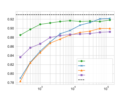
Figure 2: Test accuracy (higher the better) for a given power budget on Cifar-10 for different algorithms. LASER demonstrates consistent accuracy gains over the baselines over a wide range of power levels.

Table 3: Power required (lower the better) to reach the given target accuracy on Cifar-10. LASER requires $16\times$ lesser power than the Z-SGD to achieve the same targetaccuracy. Equivalently, LASER tolerates more channel noise than the Z-SGD for the same target accuracy as is partly supported by our theoretical analysis.

Target	Power required		Reduction
	LASER	Z-SGD
$88\%$	$250$	$4000$	$16\times$
$89\%$	$500$	$8000$	$16\times$
$90\%$	$1000$	$16000$	$16\times$
$91\%$	$2000$	$32000$	$16\times$

Setup. We consider four challenging tasks of practical interest: (i) GPT language modeling on WikiText-103, and (ii, iii, iv) image classification on Mnist, Cifar10 and Cifar100. For the language modeling, we use the GPT-2 like architecture following Pagliardini (2023) (§ F). ResNet18 is used for the Cifar datasets. For Mnist, we use a $1$-hidden-layer network for a fair comparison with Amiri & Gündüz (2020b). For distributed training of these models, we consider $k=4$ clients for language modeling and $k=16$ for image classification. We simulate the noisy channel by sampling $\boldsymbol{Z}\sim\mathcal{N}(0,\mathbf{I}_{d})$. To gauge the performance of algorithms over a wide range of noisy conditions, we vary the power $P$ geometrically in the range $[0.1,10]$ for Mnist, $[250,128000]$ for Cifar10 and Cifar100, and $[10000,1024\times 10000]$ for WikiText-103. The chosen ranges can be roughly split into low-moderate-high power regimes. Recall from noisy channel that the smaller the power, the higher the noise in the channel.

Baselines. We benchmark LASER against three different sets of baselines: (i) Z-SGD, (ii) Signum, Random-K, Sketching, and (iii) A-DSGD. Z-SGD sends the uncompressed gradients directly over the noisy channel and acts as a canonical baseline. The algorithms in (ii) are state-of-the-art distributed compression schemes for noiseless communication (Vogels et al., 2019). Signum (Bernstein et al., 2018) transmits the gradient sign followed by the majority vote and Sketching (Rothchild et al., 2020; Haddadpour et al., 2020) uses a Count Mean Sketch to compress the gradients. We omit comparison with quantization methods (Vargaftik et al., 2022) given the difference in our objectives and the settings (noisy channel). A-DSGD (Amiri & Gündüz, 2020b) is a popular compression scheme for noisy channels, relying on Top-K and random sketching. However A-DSGD does not scale to tasks of the size we consider and hence we benchmark against it only on Mnist. SGD serves as the noiseless baseline (Table 2). All the compression algorithms use the error-feedback, and use the compression factor (compressed-gradient-size/original-size) $0.2$, the optimal in the range $[0.1,0.8]$. We report the best results among $3$ independent runs for all the baselines (§ F).

4.1 Results on language modeling and image classification

For GPT language modeling, Fig. 1 in Sec. 1 highlights that LASER outperforms the baselines over a wide range of power levels. To the best of our knowledge, this is the first result of its kind to demonstrate gains for GPT training over noisy channels. Specifically, we obtain $64\%$ improvement in perplexity over Z-SGD ($76$ vs. $212$) in the low power regime ($P=10\,\mathrm{K}$) and $50\%$ ($35$ vs. $71$) for the moderate one ($P=160\,\mathrm{K}$). This demonstrates the efficacy of LASER especially in the limited power environment. Indeed, Table 1 illustrates that for a fixed target perplexity, LASER requires $16\times$ less power than the second best, Z-SGD. In the very high power regime, we observe no clear gains (as expected) compared to transmitting the uncompressed gradients directly via the Z-SGD.

We observe a similar trend for Cifar10 classification, as Fig. 2 and Table 3 demonstrate the superiority of LASER over other compression schemes; Random-K does better than the other baselines till moderate power levels after which Z-SGD dominates. Signum is considerably worse than others, as it hasn’t converged yet after $150$ epochs, and hence omitted. With regards to power reduction, Table 3 highlights that LASER requires just $(1/16)^{\text{th}}$ the power compared to Z-SGD to reach any target accuracy till $91\%$. We observe similar gains for Cifar100 (§ F).

Table 5 compares the performance of LASER against various compression algorithms on Mnist. In the very noisy regime ($P=0.1$), Random-K is slightly better than LASER and outperforms the other baselines, whereas in the moderate ($P=1$) and high power ($P=10$) regimes, LASER is slightly better than the other algorithms. On the other hand, we observe that A-DSGD performs worse than even simple compression schemes like Random-K in all the settings.

Table 4: Test accuracy (higher the better) after $50$ epochs on Mnist for low, moderate, and high power regimes.

Algorithm	Test accuracy
	$P=0.1$	$P=1$	$P=10$
Z-SGD	$81.3\%$	$87.9\%$	$91.9\%$
Signum	$76.7\%$	$83.2\%$	$85.4\%$
Random-K	${\bf 86.1\%}$	$89.3\%$	$91.5\%$
Sketching	$81.9\%$	$88.2\%$	$91.7\%$
A-DSGD	$81.6\%$	$86.9\%$	$87.3\%$
LASER	$84.3\%$	${\bf 89.9\%}$	${\bf 92.3\%}$

Table 5: Communication cost (lower the better) for GPT language modeling on WikiText-103. LASER transmits the lowest volume of data during training.

Algorithm	Data sent per iteration
Z-SGD	$496\,\mathrm{MB}$	($1\times$)
Signum	$15\,\mathrm{MB}$	($33\times$)
Random-K	$99\,\mathrm{MB}$	($5\times$)
Sketching	$99\,\mathrm{MB}$	($5\times$)
A-DSGD	$\mathrm{n/a}$	$\mathrm{n/a}$
LASER	${\bf 3\,\mathrm{\bf MB}}$	($165\times$)

4.2 Power control: static vs. dynamic policies

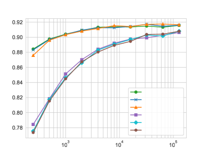
Figure 3: Accuracy vs. budget $P$ for various laws. Constant is the best for both LASER and Z-SGD.

The formulation in noisy channel allows for any power control law $P_{t}$ as long as it satisfies the average power constraint: $\sum_{t}(P_{t}/T)\leq P$. This begs a natural question: what’s the best power scheme for LASER? To answer this, for Cifar10 classification, under a fixed budget $P$ we consider different power policies with both increasing and decreasing power across epochs: the constant, piecewise constant and linear schemes. Fig. 3 illustrates the results for the decreasing power laws, while Fig. 7 their increasing counterparts. These results highlight that the constant power policy achieves the best performance for both LASER and Z-SGD, compared to the time-varying ones. Further LASER attains significant accuracy gains over Z-SGD for all the power control laws. Interestingly LASER performs the same with all the power schemes. We posit this behavior to the fact that the noisy channel already contains a time-varying noise due to the term $\frac{\max_{i}\|\|\boldsymbol{g}_{i}\|\|}{\sqrt{P_{t}}}$. Since the gradients decay over time, this inherently allows for an implicit power/SNR-control law even with a constant $P_{t}$, thus enabling the constant power scheme to fare as good as the others. Hence, without loss of generality, we consider the static power schedule for our theory and experiments. We refer to § F.7 for a detailed discussion.

4.3 Computational complexity and communication cost

Recall from Alg. 1 that the two critical components of LASER are gradient compression and channel transmission. To gauge their efficacy we analyze them via two important metrics: (i) computational complexity of compression and (ii) communication cost of transmission. For (ii), recall from Eq. (1) that the power constraint indirectly serves as a communication cost and encourages compression. Table 5 quantitatively measures the total data sent by clients for each training iteration (doesn’t change with the power $P$) for GPT language modeling on WikiText-103. As illustrated, LASER incurs the lowest communication cost among all the baselines with $165\times$ cost reduction as compared to the Z-SGD, followed by Signum which obtains $33\times$ reduction. Interestingly, LASER also achieves the best perplexity scores as highlighted in Fig. 1. For these experiments, we let rank $r=4$ for LASER and the best compression factor $0.2$ for the baselines (as detailed earlier). Signum does not require any compression factor. For (i), since LASER relies on PowerSGD for the rank decomposition, it inherits the same low-complexity benefits: Tables $3$-$7$ of Vogels et al. (2019) demonstrate that PowerSGD is efficient with significantly lower computational needs and has much smaller processing time/batch as compared to baselines without any accuracy drop. In fact, it is the core distributed algorithm behind the recent breakthrough DALL-E (§ E in Ramesh et al. (2021)).

Slow and fast fading channels. The slow/non-fading model in Eq. (1) readily generalizes to the popular fast fading channel (Guo et al., 2020; Amiri & Gündüz, 2020a): $\boldsymbol{y}=\sum_{i}\gamma_{i}\boldsymbol{x}_{i}+\boldsymbol{Z}$, where $\gamma_{i}$ are the channel fading coefficients. A standard technique here in the literature is to assume that channel-state-information (CSI) is known in the form of fading coefficients or their statistics, which essentially reduces the problem to a non-fading one. Likewise LASER can be extended to the fast fading channel as well.

Related work. (i) Compression schemes with noiseless communication. Assuming a noiseless bit pipe from clients to the server, quantization methods (Dettmers, 2015; Alistarh et al., 2017; Horvóth et al., 2022; Li et al., 2018; Wen et al., 2017; Yu et al., 2019; Vargaftik et al., 2021) quantize each coordinate and send as fewer bits as possible. Sparsification techniques (Ivkin et al., 2019; Stich et al., 2018; Sun et al., 2019; Tsuzuku et al., 2018; Wangni et al., 2018) send a reduced number of coordinates, based on criteria such as Top/Random-K, as opposed to sending the full gradient directly. Hybrid methods (Dryden et al., 2016; Lim et al., 2019) combine both. Rank compression methods (Yu et al., 2018; Cho et al., 2019; Wang et al., 2018) spectrally decompose gradient matrix (often via SVD) and transmit these factors. Since SVD is computationally prohibitive, we rely on the state-of-the-art light-weight compressor PowerSGD (Vogels et al., 2019). (ii) Compression schemes for noisy channels. The main idea here is to enable over-the-air-aggregation of gradients via the superposition nature of wireless channels (Nazer & Gastpar, 2007) thus reducing the communication latency and bandwidth. The popular A-DSGD (Amiri & Gündüz, 2020b) relies on Top-K sparsification and random sketching. However, being memory intensive, A-DSGD is restricted to Mnist with $1$-layer NN and doesn’t scale beyond. Guo et al. (2020) propose an analog-gradient-aggregation scheme but it is limited to shallow neural networks. Chang & Tandon (2020) design a digital quantizer for training over Gaussian MAC channels. (iii) Power laws. In the absence of explicit power constraints, Wei & Shen (2022a) show that $\mathcal{O}(1/t^{2})$ noise-decay ensures the standard $1/T$ convergence rate for noisy FED-AVG whereas Saha et al. (2022) propose a $t^{0.8}$ increase in SNR for the decentralized setup.

5 Conclusion

We propose a principled gradient compression scheme, LASER, for wireless distributed optimization over additive noise channels. LASER attains significant gains over its baselines on a variety of metrics such as accuracy/perplexity, complexity and communication cost. It is an interesting avenue of future research to extend LASER to channels with downlink noise and fast fading without CSI.

Impact Statement

This paper presents work whose goal is to advance the field of Machine Learning. There are many potential societal consequences of our work, none which we feel must be specifically highlighted here.

Organization. The appendix is organized as follows:

• App. A contains the requisite material for error feedback and SGD convergence analysis.

• App. B details the important technical lemmas needed for the theoretical convergence of LASER.

• App. C provides the proof for Thm 1 whereasApp. D contains the proofs of all technical lemmas.

• App. E provides additional details about the noisy channel and Alg. 1.

• App. F contains additional experimental details and results.

Appendix A Error feedback and SGD convergence toolbox

In this section we briefly recall the main techniques for the convergence analysis of SGD with error feedback (EF-SGD) from (Stich & Karimireddy, 2020). We consider $k=1$ clients with a compressor $\mathcal{C}_{r}(\cdot)$ and without any channel communication noise $\mathcal{Z}_{P}$(Sec. 2):

$$\begin{split}\boldsymbol{\theta}_{t+1}&=\boldsymbol{\theta}_{t}-\mathcal{C}_{r}(\boldsymbol{e}_{t}+\gamma_{t}\boldsymbol{g}_{t})\\ \boldsymbol{e}_{t+1}&=(\boldsymbol{e}_{t}+\gamma_{t}\boldsymbol{g}_{t})-\mathcal{C}_{r}(\boldsymbol{e}_{t}+\gamma_{t}\boldsymbol{g}_{t}).\end{split}$$ (EF-SGD)

Now we define the virtual iterates $\{\widetilde{\boldsymbol{\theta}}_{t}\}_{t\geq 0}$ which are helpful for the convergence analysis:

$$\widetilde{\boldsymbol{\theta}}_{t}\triangleq{\boldsymbol{\theta}}_{t}-\boldsymbol{e}_{t}.$$ (6)

Hence $\widetilde{\boldsymbol{\theta}}_{t+1}=\boldsymbol{\theta}_{t}-\boldsymbol{e}_{t}-\gamma_{t}\boldsymbol{g}_{t}=\widetilde{\boldsymbol{\theta}}_{t}-\gamma_{t}\boldsymbol{g}_{t}$. First we consider the case when $f$ is quasi-convex followed by the non-convex setting. In all the results below, we assume that the objective $f$ is $L$-smooth, gradient oracle $\boldsymbol{g}$ has $(M,\sigma^{2})$-bounded noise, and that $\mathcal{C}_{r}(\cdot)$ satisfies the $\delta_{r}$ compression property (Assumptions  2, 3, and 4).

$f$ is quasi-convex:

The following lemma gives a handle on the gap to optimality $\mathbb{E}{\|\widetilde{\boldsymbol{\theta}}_{t}-\boldsymbol{\theta}_{\star}\|^{2}}$.

Lemma 1 ((Stich & Karimireddy, 2020), Lemma 8).

Let $\{\boldsymbol{\theta}_{t},\boldsymbol{e}_{t}\}_{t\geq 0}$ be defined as in EF-SGD. Assume that $f$ is $\mu$-quasi convex for some $\mu\geq 0$. If $\gamma_{t}\leq\frac{1}{4L(1+M)}$ for all $t\geq 0$, then for $\{\widetilde{\boldsymbol{\theta}}_{t}\}_{t\geq 0}$ defined in Eq. (6),

$$\mathbb{E}{\|\widetilde{\boldsymbol{\theta}}_{t+1}-\boldsymbol{\theta}_{\star}\|^{2}} \leq\left(1-\frac{\mu\gamma_{t}}{2}\right)\mathbb{E}{\|\widetilde{\boldsymbol{\theta}}_{t}-\boldsymbol{\theta}_{\star}\|^{2}}-\frac{\gamma_{t}}{2}\mathbb{E}{(f(\boldsymbol{\theta}_{t})-f_{\star})}+\gamma_{t}^{2}\sigma^{2}+3L\gamma_{t}\mathbb{E}{\|\boldsymbol{\theta}_{t}-\widetilde{\boldsymbol{\theta}}_{t}\|^{2}}\,.$$ (7)

The following lemma bounds the squared norm of the error, i.e. $\mathbb{E}\|\boldsymbol{e}_{t}\|^{2}$, appearing in Eq. (7). Recall that a positive sequence $\{a_{t}\}_{t\geq 0}$ is $\tau$-slow decreasing for parameter $\tau\geq 1$ if $a_{t+1}\leq a_{t}$ and $a_{t+1}(1+1/2\tau)\geq a_{t}$. The sequence $\{a_{t}\}_{t\geq 0}$ is $\tau$-slow increasing if $\{a_{t}^{-1}\}_{t\geq 0}$ is $\tau$-slow decreasing (Stich & Karimireddy, 2020), Definition 10.

Lemma 2 ((Stich & Karimireddy, 2020), Lemma 22).

Let $\boldsymbol{e}_{t}$ be as in  (EF-SGD) for a $\delta_{r}$-approximate compressor $\mathcal{C}_{r}$ and stepsizes $\{\gamma_{t}\}_{t\geq 0}$ with $\gamma_{t+1}\leq\frac{1}{10L(2/\delta_{r}+M)}$, $\forall t\geq 0$ and $\{\gamma_{t}^{2}\}_{t\geq 0}$ $\frac{2}{\delta_{r}}$-slow decaying. Then

$$\mathbb{E}\left[3L\|\boldsymbol{e}_{t+1}\|^{2}\right]\leq\frac{\delta_{r}}{64L}\sum_{i=0}^{t}\left(1-\frac{\delta_{r}}{4}\right)^{t-i}\left(\mathbb{E}\|\nabla f(\boldsymbol{\theta}_{t-i})\|^{2}\right)+\gamma_{t}\sigma^{2}\,.$$ (8)

Furthermore, for any $\frac{4}{\delta_{r}}$-slow increasing non-negative sequence $\{w_{t}\}_{t\geq 0}$ it holds:

$$3L\sum_{t=0}^{T}w_{t}\mathbb{E}\|\boldsymbol{e}_{t}\|^{2}\leq\frac{1}{8L}\sum_{t=0}^{T}w_{t}\left(\mathbb{E}\|\nabla f(\boldsymbol{\theta}_{t})\|^{2}\right)+\sigma^{2}\sum_{t=0}^{T}w_{t}\gamma_{t}\,.$$

The following result controls the summations of the optimality gap that appear when combining Lemma 1 and Lemma 2.

Lemma 3 ((Stich & Karimireddy, 2020), Lemma 13).

For every non-negative sequence $\{r_{t}\}_{t\geq 0}$ and any parameters $d\geq a>0$, $c\geq 0$, $T\geq 0$, there exists a constant $\gamma\leq\frac{1}{d}$, such that for constant stepsizes $\{\gamma_{t}=\gamma\}_{t\geq 0}$ and weights $w_{t}:=(1-a\gamma)^{-(t+1)}$ it holds

$$\Psi_{T}:=\frac{1}{W_{T}}\sum_{t=0}^{T}\left(\frac{w_{t}}{\gamma_{t}}\left(1-a\gamma_{t}\right)r_{t}-\frac{w_{t}}{\gamma_{t}}r_{t+1}+c\gamma_{t}w_{t}\right)=\widetilde{\cal{O}}\left(dr_{0}\exp\left[-\frac{aT}{d}\right]+\frac{c}{aT}\right)\,.$$

Combining the above lemmas, we obtain the following result for the convergence rate of EF-SGD.

Theorem 2 ((Stich & Karimireddy, 2020), Theorem 22).

Let $\{\boldsymbol{\theta}_{t}\}_{t\geq 0}$ denote the iterates of the error compensated stochastic gradient descent (EF-SGD) with constant stepsize $\{\gamma_{t}=\gamma\}_{t\geq 0}$ and with a $\delta_{r}$-approximate compressor on a differentiable function $f\colon\mathbb{R}^{d}\to\mathbb{R}$ under Assumptions 2 and 3. Then, if $f$

• satisfies Assumption 1 for $\mu>0$, then there exists a stepsize $\gamma\leq\frac{1}{10L(2/\delta_{r}+M)}$ (chosen as in Lemma 3) such that where the output $\boldsymbol{\theta}_{\rm out}\in\{\boldsymbol{\theta}_{t}\}_{t=0}^{T-1}$ is chosen to be $\boldsymbol{\theta}_{t}$ with probability proportional to $(1-\mu\gamma/2)^{-t}$.

• satisfies Assumption 1 for $\mu=0$, then there exists a stepsize $\gamma\leq\frac{1}{10L(2/\delta_{r}+M)}$ (chosen as in Lemma 3) such that

  $$\mathbb{E}f(\boldsymbol{\theta}_{\rm out})-f_{*}=\mathcal{O}\left(\frac{L(1/\delta_{r}+M)\|\boldsymbol{\theta}_{0}-\boldsymbol{\theta}_{\star}\|^{2}}{T}+\frac{\sigma\|\boldsymbol{\theta}_{0}-\boldsymbol{\theta}_{\star}\|}{\sqrt{T}}\right)\,,$$

  where the output $\boldsymbol{\theta}_{\rm out}\in\{\boldsymbol{\theta}_{t}\}_{t=0}^{T-1}$ is chosen uniformly at random from the iterates $\{\boldsymbol{\theta}_{t}\}_{t=0}^{T-1}$.

$f$ is non-convex:

Now we consider the case where $f$ is an arbitrary non-convex function. The above set of results extend in a similar fashion to this setting too as described below:

Lemma 4 ((Stich & Karimireddy, 2020), Lemma 9).

Let $\{\boldsymbol{\theta}_{t},\boldsymbol{e}_{t}\}_{t\geq 0}$ be defined as in EF-SGD. If $\gamma_{t}\leq\frac{1}{2L(1+M)}$ for all $t\geq 0$, then for $\{\widetilde{\boldsymbol{\theta}}_{t}\}_{t\geq 0}$ defined in Eq. (6),

$$\mathbb{E}[f(\widetilde{\boldsymbol{\theta}}_{t+1})]\leq\mathbb{E}[f(\widetilde{\boldsymbol{\theta}}_{t})]-\frac{\gamma_{t}}{4}\mathbb{E}\|\nabla f(\boldsymbol{\theta}_{t})\|^{2}+\frac{\gamma_{t}^{2}L\sigma^{2}}{2}+\frac{\gamma_{t}L^{2}}{2}\mathbb{E}\|\boldsymbol{\theta}_{t}-\widetilde{\boldsymbol{\theta}}_{t}\|^{2}\,.$$ (9)

Lemma 5 ((Stich & Karimireddy, 2020), Lemma 22).

Let $\boldsymbol{e}_{t}$ be as in  (EF-SGD) for a $\delta_{r}$-approximate compressor $\mathcal{C}_{r}$ and stepsizes $\{\gamma_{t}\}_{t\geq 0}$ with $\gamma_{t+1}\leq\frac{1}{10L(2/\delta_{r}+M)}$, $\forall t\geq 0$ and $\{\gamma_{t}^{2}\}_{t\geq 0}$ $\frac{2}{\delta_{r}}$-slow decaying. Then

$$\mathbb{E}\left[3L\|\boldsymbol{e}_{t+1}\|^{2}\right]\leq\frac{\delta_{r}}{64L}\sum_{i=0}^{t}\left(1-\frac{\delta_{r}}{4}\right)^{t-i}\left(\mathbb{E}\|\nabla f(\boldsymbol{\theta}_{t-i})\|^{2}\right)+\gamma_{t}\sigma^{2}\,.$$ (10)

Furthermore, for any $\frac{4}{\delta_{r}}$-slow increasing non-negative sequence $\{w_{t}\}_{t\geq 0}$ it holds:

$$3L\sum_{t=0}^{T}w_{t}\mathbb{E}\|\boldsymbol{e}_{t}\|^{2}\leq\frac{1}{8L}\sum_{t=0}^{T}w_{t}\left(\mathbb{E}\|\nabla f(\boldsymbol{\theta}_{t-i})\|^{2}\right)+\sigma^{2}\sum_{t=0}^{T}w_{t}\gamma_{t}\,.$$

Lemma 6 ((Stich & Karimireddy, 2020), Lemma 14).

For every non-negative sequence $\{r_{t}\}_{t\geq 0}$ and any parameters $d\geq 0$, $c\geq 0$, $T\geq 0$, there exists a constant $\gamma\leq\frac{1}{d}$, such that for constant stepsizes $\{\gamma_{t}=\gamma\}_{t\geq 0}$ it holds:

$$\Psi_{T}:=\frac{1}{T+1}\sum_{t=0}^{T}\left(\frac{r_{t}}{\gamma_{t}}-\frac{r_{t+1}}{\gamma_{t}}+c\gamma_{t}\right)\leq\frac{dr_{0}}{T+1}+\frac{2\sqrt{cr_{0}}}{\sqrt{T+1}}\,.$$

Now we have the final convergence result for the non-convex setting.

Theorem 3 ((Stich & Karimireddy, 2020), Theorem 22).

Let $\{\boldsymbol{\theta}_{t}\}_{t\geq 0}$ denote the iterates of the error compensated stochastic gradient descent (EF-SGD) with constant stepsize $\{\gamma_{t}=\gamma\}_{t\geq 0}$ and with a $\delta_{r}$-approximate compressor on a differentiable function $f\colon\mathbb{R}^{d}\to\mathbb{R}$ under Assumptions 2 and 3. Then, if $f$ is an arbitrary non-convex function, there exists a stepsize $\gamma\leq\frac{1}{10L(1/\delta_{r}+M)}$ (chosen as in Lemma 6), such that

$$\mathbb{E}\|\nabla f(\boldsymbol{\theta}_{\rm out})\|^{2}=\mathcal{O}\left(\frac{L(1/\delta_{r}+M)(f(\boldsymbol{\theta}_{0})-f_{\star})}{T}+\sigma\sqrt{\frac{L(f(\boldsymbol{\theta}_{0})-f_{\star})}{T}}\right)\,.$$

where the output $\boldsymbol{\theta}_{\rm out}\in\{\boldsymbol{\theta}_{t}\}_{t=0}^{T-1}$ is chosen uniformly at random from the iterates $\{\boldsymbol{\theta}_{t}\}_{t=0}^{T-1}$.

Appendix B Technical lemmas for LASER convergence

Towards the convergence analysis of LASER for $k=1$, we rewrite the Alg. 1 succinctly as:

$$\begin{split}\boldsymbol{\theta}_{t+1}&=\boldsymbol{\theta}_{t}-\mathcal{Z}_{(\boldsymbol{\alpha},\boldsymbol{\beta})}\left(\mathcal{C}_{r}(\boldsymbol{e}_{t}+\gamma_{t}\boldsymbol{g}_{t})\right)\\ \boldsymbol{e}_{t+1}&=(\boldsymbol{e}_{t}+\gamma_{t}\boldsymbol{g}_{t})-\mathcal{C}_{r}(\boldsymbol{e}_{t}+\gamma_{t}\boldsymbol{g}_{t})\,,\end{split}$$ (LASER)

where the channel corrupted gradient approximation $\mathcal{Z}_{(\boldsymbol{\alpha},\boldsymbol{\beta})}(\cdot)$ is given by

$$\mathcal{Z}_{(\boldsymbol{\alpha},\boldsymbol{\beta})}(\underbrace{\mathcal{C}_{r}(\boldsymbol{e}_{t}+\gamma_{t}\boldsymbol{g}_{t})}_{=\boldsymbol{P}\boldsymbol{Q}^{\top}})\triangleq\sum_{i=1}^{r}\left(\boldsymbol{p}_{i}+\frac{\|\boldsymbol{p}_{i}\|}{\sqrt{\alpha_{i}}}\cdot\boldsymbol{Z}_{m}^{(i)}\right)\left(\boldsymbol{q}_{i}+\frac{\|\boldsymbol{q}_{i}\|}{\sqrt{\beta_{i}}}\cdot\boldsymbol{Z}_{n}^{(i)}\right)^{\top},$$ (11)

and $\boldsymbol{\alpha}=(\alpha_{i})_{i=1}^{r}$ and $\boldsymbol{\beta}=(\beta_{i})_{i=1}^{r}$ are appropriate power allocations to transmit the respective left and right factors $\boldsymbol{P}=[\boldsymbol{p}_{1},\ldots,\boldsymbol{p}_{r}]\in\mathbb{R}^{m\times r}$ and $\boldsymbol{Q}=[\boldsymbol{q}_{1},\ldots,\boldsymbol{q}_{r}]\in\mathbb{R}^{n\times r}$ for the decomposition $\mathcal{C}_{r}(\boldsymbol{e}_{t}+\gamma_{t}\boldsymbol{g}_{t})=\boldsymbol{P}\boldsymbol{Q}^{\top}$. $\boldsymbol{Z}_{m}^{(i)}\in\mathbb{R}^{m}$ and $\boldsymbol{Z}_{n}^{(i)}\in\mathbb{R}^{n}$ denote the independent channel noises for each factor $i\in[r]$.

Thus we observe from LASER that it has an additional channel corruption in the form of $\mathcal{Z}_{(\boldsymbol{\alpha},\boldsymbol{\beta})}(\cdot)$ as compared to the EF-SGD. Now in the remainder of this section, we explain how to choose the power allocation $(\boldsymbol{\alpha},\boldsymbol{\beta})$ (App. B.1), how to control the influence of the channel $\mathcal{Z}_{(\boldsymbol{\alpha},\boldsymbol{\beta})}(\cdot)$ on the convergence of LASER (App. B.2), and utilize these results to establish technical lemmas along the lines of App. A for LASER (App. B.3).

B.1 Power allocation

In this section, we introduce the key technical lemmas about power allocation that are crucial for the theoretical results. We start with the rank one case.

Lemma 7 (Rank-$1$ power allocation).

For a power $P>0$ and $m,n\in\mathbb{N}$ with $m\leq n$, define the function $f_{P}:\mathbb{R}_{+}\times\mathbb{R}_{+}\to\mathbb{R}_{+}$ as

$$f_{P}(\alpha,\beta)\triangleq\left(1+\frac{m}{\alpha}\right)\left(1+\frac{n}{\beta}\right),$$

and the constraint set $S_{P}\triangleq\left\{(\alpha,\beta):\alpha\geq 0,\beta\geq 0,\alpha+\beta=P\right\}$. Then for the minimizer $(\alpha^{\star},\beta^{\star})=\mathop{\operatorname{argmin}}_{(\alpha,\beta)\in S_{P}}f_{P}(\alpha,\beta)$, we have

$$f_{P}(\alpha^{\star},\beta^{\star})\leq 1+\frac{4}{m\,\mathrm{SNR}}\left(1+\frac{1}{n\,\mathrm{SNR}}\right),\quad\mathrm{SNR}\triangleq\frac{P}{mn}\,.$$

Further the minimizer is given by

$$\alpha^{\star} =\begin{cases}\sqrt{1+\frac{P}{n}}\left(\frac{\sqrt{1+\frac{P}{m}}-\sqrt{1+\frac{P}{n}}}{\frac{1}{m}-\frac{1}{n}}\right),&m\neq n\\ P/2,&m=n\end{cases}$$

$$\beta^{\star} =P-\alpha^{\star}.$$

Lemma 8 (Rank-$r$ power allocation).

For a power $P>0$, $m,n,r\in\mathbb{N}$ with $m\leq n$, and positive scalars $\kappa_{1},\ldots,\kappa_{r}>0$ with $\sum_{i}\kappa_{i}=1$, define the function $f_{P}:(\mathbb{R}_{+})^{r}\times(\mathbb{R}_{+})^{r}\to\mathbb{R}_{+}$ as

$$f_{P}(\boldsymbol{\alpha},\boldsymbol{\beta})\triangleq\sum_{i=1}^{r}\kappa_{i}\left(1+\frac{m}{\alpha_{i}}\right)\left(1+\frac{n}{\beta_{i}}\right),\quad\boldsymbol{\alpha}=(\alpha_{i})_{i=1}^{r},\,\boldsymbol{\beta}=(\beta_{i})_{i=1}^{r},$$

and the constraint set $S_{P}\triangleq\left\{\{(\boldsymbol{\alpha},\boldsymbol{\beta}):\boldsymbol{\alpha}\geq 0,\boldsymbol{\beta}\geq 0,\sum_{i}(\alpha_{i}+\beta_{i})=P\right\}$. Then there exists a power allocation scheme $(\boldsymbol{\alpha}^{\star},\boldsymbol{\beta}^{\star})\in S_{P}$ such that

$$\min_{(\boldsymbol{\alpha},\boldsymbol{\beta})\in S_{P}}f_{P}(\boldsymbol{\alpha},\boldsymbol{\beta})\leq f_{P}(\boldsymbol{\alpha}^{\star},\boldsymbol{\beta}^{\star})\leq 1+\frac{4}{(m/r)\,\mathrm{SNR}}\left(1+\frac{1}{(n/r)\,\mathrm{SNR}}\right),$$

where $\mathrm{SNR}\triangleq\frac{P}{mn}$. Further $(\boldsymbol{\alpha}^{\star},\boldsymbol{\beta}^{\star})$ is given by

$$\alpha_{i}^{\star} =\begin{cases}\sqrt{1+\frac{P_{i}}{n}}\left(\frac{\sqrt{1+\frac{P_{i}}{m}}-\sqrt{1+\frac{P_{i}}{n}}}{\frac{1}{m}-\frac{1}{n}}\right),&m\neq n\\ P_{i}/2,&m=n\end{cases}$$

$$\beta_{i}^{\star} =P_{i}-\alpha_{i}^{\star},$$

$$P_{i} =P\left(\frac{\sqrt{\kappa_{i}}}{\sum_{j}\sqrt{\kappa_{j}}}\right).$$

Remark 1.

In other words, we first divide the power $P$ proportional to $\sqrt{\kappa_{i}}$ for each $i\in[r]$ and further allocate this $P_{i}$ amongst $\alpha_{i}^{\star}$ and $\beta_{i}^{\star}$ as per the optimal rank one allocation scheme in Lemma 7.

B.2 Channel influence factor

In this section we establish the bounds for the channel influence defined in Eq. (4) for both Z-SGD and LASER. This helps us give a handle to control the second moment of the gradient corrupted by channel noise.

Lemma 9 (Channel influence on Z-SGD).

For the Z-SGD algorithm that sends the uncompressed gradients directly over the noisy channel with power constraint $P$, we have

$$\lambda_{\textsc{Z-SGD}}=\frac{1}{\mathrm{SNR}},$$ (12)

where $\mathrm{SNR}=\frac{P}{mn}$.

Lemma 10.

For the LASER algorithm with the optimal power allocation $(\boldsymbol{\alpha},\boldsymbol{\beta})$ (chosen as in Lemma 8), we have

$$\lambda_{\textsc{LASER}}\leq\frac{4}{(m/r)\,\mathrm{SNR}}\left(1+\frac{1}{(n/r)\,\mathrm{SNR}}\right),$$ (13)

where $\mathrm{SNR}=\frac{P}{mn}$.

Remark 2.

Note that for the optimal power allocation via Lemma 8, we need the positive scalars $\kappa_{1},\ldots,\kappa_{r}$. In the context of LASER, we will later see in the proof in App. D that $\kappa_{i}\propto\|\boldsymbol{p}_{i}\|^{2}$.

Thus Lemma 9 and Lemma 10 establish that

$$\lambda_{\textsc{LASER}}\leq\frac{4}{(m/r)\,\mathrm{SNR}}\left(1+\frac{1}{(n/r)\,\mathrm{SNR}}\right)\ll\frac{1}{\mathrm{SNR}}=\lambda_{\textsc{Z-SGD}}.$$

In the low-rank (Vogels et al., 2019) and constant-order SNR regime where $r=\mathcal{O}(1)$ and $\mathrm{SNR}=\Omega(1)$, we observe that $\lambda_{\textsc{LASER}}$ is roughly $\mathcal{O}(m)$ times smaller than $\lambda_{\textsc{Z-SGD}}$.

Note on assumption between $\lambda_{\textsc{LASER}}$ and $\delta_{r}$. Recall from LASER that the local memory $\boldsymbol{e}_{t}$ has only access to the compressed gradients and not the channel output. In an hypothetical scenario, where it has access to the same, it follows that $\mathbb{E}_{\boldsymbol{Z}}\|\mathcal{Z}_{(\boldsymbol{\alpha},\boldsymbol{\beta})}(\mathcal{C}_{r}(\boldsymbol{M}))-\boldsymbol{M}\|^{2}\leq(1-(\delta_{r}-\lambda_{\textsc{LASER}}))\|\boldsymbol{M}\|^{2}$. Hence for the compression property in this ideal scenario, we need $\lambda_{\textsc{LASER}}\leq\delta_{r}$.

B.3 Optimality gap and error bounds for  LASER iterates

In this section, we characterize the gap to the optimality and the error norm for the LASER iterates $\{\boldsymbol{\theta}_{t}\}_{t\geq 0}$ (similar to Lemmas  1, 2, 2 and 5 for EF-SGD). Towards the same, first we define the virtual iterates $\{\widetilde{\boldsymbol{\theta}_{t}}\}_{t\geq 0}$ as follows:

$$\widetilde{\boldsymbol{\theta}}_{t}\triangleq{\boldsymbol{\theta}}_{t}-\boldsymbol{e}_{t}\,.$$ (14)

Thus,

$$\widetilde{\boldsymbol{\theta}}_{t+1}={\boldsymbol{\theta}}_{t+1}-\boldsymbol{e}_{t+1}=\widetilde{\boldsymbol{\theta}}_{t}-\gamma_{t}\boldsymbol{g}_{t}+\mathcal{C}_{r}(\boldsymbol{e}_{t}+\gamma_{t}\boldsymbol{g}_{t})-\mathcal{Z}_{(\boldsymbol{\alpha},\boldsymbol{\beta})}\left(\mathcal{C}_{r}(\boldsymbol{e}_{t}+\gamma_{t}\boldsymbol{g}_{t})\right).$$ (15)

The following lemma controls the optimality gap $\mathbb{E}\|\widetilde{\boldsymbol{\theta}}_{t}-\boldsymbol{\theta}_{\star}\|^{2}$ when $f$ is quasi-convex.

Lemma 11 (Descent for quasi-convex).

Let $\{\boldsymbol{\theta}_{t},\boldsymbol{e}_{t}\}_{t\geq 0}$ be defined as in LASER. Assume that $f$ is $\mu$-quasi convex for some $\mu\geq 0$ and that Assumptions 2 and 3 hold. If $\gamma_{t}\leq\frac{1}{4L(1+M)}\,\left(\frac{1-2\lambda_{\textsc{LASER}}}{1+\lambda_{\textsc{LASER}}}\right)$ for all $t\geq 0$, then for $\{\widetilde{\boldsymbol{\theta}}_{t}\}_{t\geq 0}$ defined in Eq. (14),

$$\begin{split}\mathbb{E}{\|\widetilde{\boldsymbol{\theta}}_{t+1}-\boldsymbol{\theta}_{\star}\|^{2}}&\leq\left(1-\frac{\mu\gamma_{t}}{2}\right)\mathbb{E}{\|\widetilde{\boldsymbol{\theta}}_{t}-\boldsymbol{\theta}_{\star}\|^{2}}-\frac{\gamma_{t}}{2}\mathbb{E}{(f(\boldsymbol{\theta}_{t})-f_{\star})}+\gamma_{t}^{2}\sigma^{2}(1+\lambda_{\textsc{LASER}})\\ &\hskip 90.00014pt+(3L\gamma_{t}(1+\lambda_{\textsc{LASER}})+\lambda_{\textsc{LASER}})\mathbb{E}{\|\boldsymbol{\theta}_{t}-\widetilde{\boldsymbol{\theta}}_{t}\|^{2}}\,.\end{split}$$ (16)

Notice that Lemma 11 is similar to Lemma 1 for noiseless EF-SGD except for an additional channel influence factor $\lambda_{\textsc{LASER}}$. The following result bounds the error norm.

Lemma 12 (Error control).

Let $\boldsymbol{e}_{t}$ be as in  (LASER) for a $\delta_{r}$-approximate compressor $\mathcal{C}_{r}$ and stepsizes $\{\gamma_{t}\}_{t\geq 0}$ with $\gamma_{t}\leq\frac{1}{10L(2/\delta_{r}+M)(1+\lambda_{\textsc{LASER}})}$, $\forall t\geq 0$ and $\{\gamma_{t}^{2}\}_{t\geq 0}$ $\frac{2}{\delta_{r}}$-slow decaying. Further suppose that Assumption 5 holds. Then

$$\begin{split}\left(3L(1+\lambda_{\textsc{LASER}})+\frac{\lambda_{\textsc{LASER}}}{\gamma_{t}}\right)\mathbb{E}\|\boldsymbol{e}_{t+1}\|^{2}&\leq\frac{\delta_{r}}{32L}\sum_{i=0}^{t}\left(1-\frac{\delta_{r}}{4}\right)^{t-i}\left(\mathbb{E}\|\nabla f(\boldsymbol{\theta}_{t-i})\|^{2}\right)\\ &\hskip 80.00012pt+\gamma_{t}\sigma^{2}(1+\lambda_{\textsc{LASER}})\,.\end{split}$$ (17)

Furthermore, for any $\frac{4}{\delta_{r}}$-slow increasing non-negative sequence $\{w_{t}\}_{t\geq 0}$ it holds:

$$\begin{split}\left(3L(1+\lambda_{\textsc{LASER}})+\frac{\lambda_{\textsc{LASER}}}{\gamma_{t}}\right)\sum_{t=0}^{T}w_{t}\mathbb{E}\|\boldsymbol{e}_{t}\|^{2}&\leq\frac{1}{6L}\sum_{t=0}^{T}w_{t}\left(\mathbb{E}\|\nabla f(\boldsymbol{\theta}_{t})\|^{2}\right)\\ &\hskip 10.00002pt+\sigma^{2}(1+\lambda_{\textsc{LASER}})\sum_{t=0}^{T}w_{t}\gamma_{t}\,.\end{split}$$ (18)

The following lemma establishes the progress in the descent for non-convex case.

Lemma 13 (Descent for non-convex).

Let $\{\boldsymbol{\theta}_{t},\boldsymbol{e}_{t}\}_{t\geq 0}$ be defined as in LASER and that Assumptions 2 and 3 hold. If $\gamma_{t}\leq\frac{1}{4L(1+M)(1+\lambda_{\textsc{LASER}})}$ for all $t\geq 0$, then for $\{\widetilde{\boldsymbol{\theta}}_{t}\}_{t\geq 0}$ defined in Eq. (14),

$$\begin{split}\mathbb{E}[f(\widetilde{\boldsymbol{\theta}}_{t+1})]&\leq\mathbb{E}[f(\widetilde{\boldsymbol{\theta}}_{t})]-\frac{\gamma_{t}}{4}\mathbb{E}\|\nabla f(\boldsymbol{\theta}_{t})\|^{2}+\frac{\gamma_{t}^{2}L\sigma^{2}(1+\lambda_{\textsc{LASER}})}{2}\\ &\hskip 70.0001pt+\mathbb{E}\|\boldsymbol{\theta}_{t}-\widetilde{\boldsymbol{\theta}}_{t}\|^{2}\left(\frac{L^{2}\gamma_{t}}{2}+L\lambda_{\textsc{LASER}}\right).\end{split}$$ (19)

Appendix C Proof of Thm 1

Proof.

We prove the bounds in (i) and (ii) when $f$ is quasi-convex, (iii) when $f$ is an arbitrary non-convex function, and (iv) for Z-SGD.

(i), (ii) $f$ is $\mu$-quasi-convex: Observe that the assumptions of Thm 1 automatically satisfy the conditions of Lemma 11. Denoting $r_{t}\triangleq\mathbb{E}{\|\widetilde{\boldsymbol{\theta}}_{t+1}-\boldsymbol{\theta}_{\star}\|^{2}}$ and $s_{t}\triangleq\mathbb{E}{(f(\boldsymbol{\theta}_{t})-f_{\star})}$, for any $w_{t}>0$ we obtain

$$\frac{w_{t}}{2}s_{t}\stackrel{{\scriptstyle\eqref{eq:missquasi_progress}}}{{\leq}}\frac{w_{t}}{\gamma_{t}}\left(1-\frac{\mu\gamma_{t}}{2}\right)r_{t}-\frac{w_{t}}{\gamma_{t}}r_{t+1}+\gamma_{t}w_{t}\sigma^{2}(1+\lambda_{\textsc{LASER}})+3w_{t}(L(1+\lambda_{\textsc{LASER}})+\frac{\lambda_{\textsc{LASER}}}{\gamma_{t}})\mathbb{E}\|\boldsymbol{e}_{t}\|^{2}\,.$$

Taking summation on both sides and invoking Lemma 2 (assumption on $w_{t}$ verified below),

$$\sum_{t=0}^{T}\frac{w_{t}}{2}s_{t}\stackrel{{\scriptstyle\eqref{eq:misserrorsum_control}}}{{\leq}}\sum_{t=0}^{T}\left(\frac{w_{t}}{\gamma_{t}}\left(1-\frac{\mu\gamma_{t}}{2}\right)r_{t}-\frac{w_{t}}{\gamma_{t}}r_{t+1}+2\gamma_{t}w_{t}\sigma^{2}(1+\lambda_{\textsc{LASER}})\right)+\frac{1}{6L}\sum_{t=0}^{T}w_{t}\left(\mathbb{E}\|\nabla f(\boldsymbol{\theta}_{t})\|^{2}\right).$$

Since $f$ is $L$-smooth, we have $\|\nabla f(\boldsymbol{\theta}_{t})\|^{2}\leq 2L(f(\boldsymbol{\theta}_{t})-f_{\star})$. Now rewriting the above inequality, we have

$$\frac{1}{6}\sum_{t=0}^{T}w_{t}s_{t}\leq\sum_{t=0}^{T}\left(\frac{w_{t}}{\gamma_{t}}\left(1-\frac{\mu\gamma_{t}}{2}\right)r_{t}-\frac{w_{t}}{\gamma_{t}}r_{t+1}+2\gamma_{t}w_{t}\sigma^{2}(1+\lambda_{\textsc{LASER}})\right).$$

Substituting $W_{T}\triangleq\sum_{t=0}^{T}w_{t}$,

$$\frac{1}{W_{T}}\sum_{t=0}^{T}w_{t}s_{t}\leq\frac{6}{W_{T}}\sum_{t=0}^{T}\left(\frac{w_{t}}{\gamma_{t}}\left(1-\frac{\mu\gamma_{t}}{2}\right)r_{t}-\frac{w_{t}}{\gamma_{t}}r_{t+1}+2\gamma_{t}w_{t}\sigma^{2}(1+\lambda_{\textsc{LASER}})\right)=:\Xi_{T}\,.$$

Now it remains to derive the estimate for $\Xi_{T}$. Towards this, (i) if $\mu>0$ and with constant stepsize $\gamma_{t}=\gamma\leq\frac{1}{10L(\frac{2}{\delta_{r}}+M)(1+\lambda_{\textsc{LASER}})}$, we observe that $(1-\frac{\mu\gamma}{2})\geq\left(1-\frac{\delta_{r}}{16}\right)$ and by Example 1 in (Stich & Karimireddy, 2020), the weights $w_{t}=\left(1-\frac{\mu\gamma}{2}\right)^{-(t+1)}$ are $2\tau$-slow increasing with $\tau=\frac{2}{\delta_{r}}$. Hence the claim in (i) follows by applying Lemma 3 and observing that the sampling probablity to choose $\boldsymbol{\theta}_{\rm out}$ from $\{\boldsymbol{\theta}_{t}\}_{t=0}^{T-1}$ is same as $w_{t}$.

For (ii) with constant stepsize and $\mu=0$, we apply Lemma 6 by setting the weights $w_{t}=1$.

(iii) $f$ is non-convex The proof in this case is very similar to that of the above. Denoting $r_{t}\triangleq 4\mathbb{E}[f(\widetilde{\boldsymbol{\theta}}_{t})-f_{\star}],s_{t}\triangleq\mathbb{E}\|\nabla f(\boldsymbol{\theta}_{t})\|^{2},c=4L\sigma^{2}(1+\lambda_{\textsc{LASER}})$, and $w_{t}=1$, we have from Lemma 13 that

$$\frac{s_{t}}{4}\stackrel{{\scriptstyle\eqref{eq:missnoncvx_progress}}}{{\leq}}\frac{r_{t}}{4\gamma_{t}}-\frac{r_{t+1}}{4\gamma_{t}}+\frac{\gamma_{t}c}{8}+L\left(\frac{L}{2}+\frac{\lambda_{\textsc{LASER}}}{\gamma_{t}}\right)\mathbb{E}\|\boldsymbol{e}_{t}\|^{2}.$$

Since $\frac{L}{2}\leq 3L(1+\lambda_{\textsc{LASER}})$, multiplying both sides of the above inequality by $w_{t}$ and taking summation, we obtain

$$\frac{1}{4W_{T}}\sum_{t=0}^{T}w_{t}s_{t}\stackrel{{\scriptstyle\eqref{eq:misserrorsum_control}}}{{\leq}}\frac{1}{W_{T}}\sum_{t=0}^{T}w_{t}\left(\frac{r_{t}}{4\gamma_{t}}-\frac{r_{t+1}}{4\gamma_{t}}+\frac{\gamma_{t}c}{8}\right)+\frac{L}{W_{T}}\left(\sum_{t=0}^{T}\frac{w_{t}s_{t}}{6L}+\frac{cw_{t}\gamma_{t}}{4L}\right),$$

which upon rearranging gives

$$\frac{1}{W_{T}}\sum_{t=0}^{T}w_{t}s_{t}{\leq}\frac{12}{W_{T}}\sum_{t=0}^{T}w_{t}\left(\frac{r_{t}}{4\gamma_{t}}-\frac{r_{t+1}}{4\gamma_{t}}+\frac{3\gamma_{t}c}{8}\right).$$

Now invoking Lemma 6 yields the final result in (iii).

Z-SGD: Recall from  Z-SGD that the iterates $\{\boldsymbol{\theta}_{t}\}_{t\geq 0}$ are given by

$$\boldsymbol{\theta}_{t+1}=\boldsymbol{\theta}_{t}-\gamma_{t}\,\mathcal{Z}_{P}(\boldsymbol{g}_{t}).$$

Thus Z-SGD can be thought of as a special case of EF-SGD with no compression, i.e. $\delta_{r}=1$, and hence we can utilize the same convergence tools. It remains to estimate the first and second moments of the stochastic gradient $\mathcal{Z}_{P}(\boldsymbol{g}_{t})$. Recall from the definition of $\mathcal{Z}_{P}$ in the  noisy channel that $\mathcal{Z}_{P}(\boldsymbol{g}_{t})=\boldsymbol{g}_{t}+\frac{\|\boldsymbol{g}_{t}\|}{\sqrt{P}}\,\boldsymbol{Z}_{t}$, where $\boldsymbol{Z}_{t}$ is a zero-mean independent channel noise, and from Assumption 3 that $\boldsymbol{g}_{t}=\nabla f(\boldsymbol{\theta}_{t})+\boldsymbol{\xi}_{t}$ with a $(M,\sigma^{2})$-bounded noise $\boldsymbol{\xi}_{t}$. Hence

$$\mathbb{E}\left[\mathcal{Z}_{P}(\boldsymbol{g}_{t})|\boldsymbol{\theta}_{t}\right] =\mathbb{E}[\boldsymbol{g}_{t}|\boldsymbol{\theta}_{t}]=\nabla f(\boldsymbol{\theta}_{t}),$$

$$\mathbb{E}\left[\|\mathcal{Z}_{P}(\boldsymbol{g}_{t})-\nabla f(\boldsymbol{\theta}_{t})\|^{2}|\boldsymbol{\theta}_{t}\right] =\mathbb{E}\left[\|\mathcal{Z}_{P}(\boldsymbol{g}_{t})-\boldsymbol{g}_{t}+\boldsymbol{g}_{t}-\nabla f(\boldsymbol{\theta}_{t})\|^{2}|\boldsymbol{\theta}_{t}\right]$$

$$=\mathbb{E}\left[\|\mathcal{Z}_{P}(\boldsymbol{g}_{t})-\boldsymbol{g}_{t}\|^{2}|\boldsymbol{\theta}_{t}\right]+\mathbb{E}\left[\|\boldsymbol{g}_{t}-\nabla f(\boldsymbol{\theta}_{t})\|^{2}|\boldsymbol{\theta}_{t}\right]$$

$$\stackrel{{\scriptstyle~{}\ref{eq:chanel_infl}}}{{=}}\mathbb{E}\left[\lambda_{\textsc{Z-SGD}}\|\boldsymbol{g}_{t}\|^{2}|\boldsymbol{\theta}_{t}\right]+\mathbb{E}\|\boldsymbol{\xi}_{t}\|^{2}$$

$$=\lambda_{\textsc{Z-SGD}}\|\nabla f(\boldsymbol{\theta}_{t})\|^{2}+(1+\lambda_{\textsc{Z-SGD}})\mathbb{E}\|\boldsymbol{\xi}_{t}\|^{2}$$

$$\leq(M+1)(1+\lambda_{\textsc{Z-SGD}})\|\nabla f(\boldsymbol{\theta}_{t})\|^{2}+(1+\lambda_{\textsc{Z-SGD}})\sigma^{2}.$$

Thus Z-SGD satifies the $(\widetilde{M},\widetilde{\sigma}^{2})$-bounded noise condition in Assumption 3 with $\widetilde{M}=(M+1)(1+\lambda_{\textsc{Z-SGD}})$ and $\widetilde{\sigma}^{2}=(1+\lambda_{\textsc{Z-SGD}})\sigma^{2}$. Thus the claim (iv) follows from applying Thm 2 and Thm 3 with the constants $\delta_{r}\rightarrow 1,M\rightarrow\widetilde{M},\sigma^{2}\rightarrow\widetilde{\sigma}^{2}$.

Finally, Lemma 9 and Lemma 10 establish the relation between the channel influence factors $\lambda_{\textsc{Z-SGD}}$ and $\lambda_{\textsc{LASER}}$.

∎

Appendix D Proof of technical lemmas

D.1 Proof of Lemma 7

Proof.

Since $\log(\cdot)$ is a monotonic function, minimizing $f_{P}(\alpha,\beta)$ over $S_{P}=\left\{(\alpha,\beta):\alpha\geq 0,\beta\geq 0,\alpha+\beta=P\right\}$ is equivalent to minimizing $\log f_{P}(\alpha,\beta)=\log\left(1+\frac{m}{\alpha}\right)+\log\left(1+\frac{n}{\beta}\right)$. Define the Lagrangian $L(\alpha,\beta,\lambda)$ as

$$L(\alpha,\beta,\lambda)\triangleq\log\left(1+\frac{m}{\alpha}\right)+\log\left(1+\frac{n}{\beta}\right)+\lambda(\alpha+\beta-P).$$

Letting $\nabla_{\alpha}L=\nabla_{\beta}L=0$, we obtain that $\frac{m}{\alpha(m+\alpha)}=\frac{n}{\beta(n+\beta)}$. Now constraining $\alpha+\beta=P$, we obtain the following quadratic equation:

$$\alpha^{2}\left(\frac{1}{m}-\frac{1}{n}\right)+2\alpha\left(1+\frac{P}{n}\right)-\left(\frac{P^{2}}{n}+P\right)=0.$$

If $m=n$, the solution is given by $\alpha^{\star}=\beta^{\star}=P/2$. If $m\neq n$, the solution is given by

$$\alpha^{\star} =\sqrt{1+\frac{P}{n}}\left(\frac{\sqrt{1+\frac{P}{m}}-\sqrt{1+\frac{P}{n}}}{\frac{1}{m}-\frac{1}{n}}\right),$$ (20)

$$\beta^{\star} =P-\alpha^{\star}.$$

It is easy to verify that $(\alpha^{\star},\beta^{\star})$ is the unique minimizer to $f_{P}$ since it’s convex over $S_{P}$. Now it remains to show the upper bound for $f_{P}(\alpha^{\star},\beta^{\star})$. Without loss of generality, in the reminder of the proof we assume $m<n$ and denote $\alpha^{\star}$ by simply $\alpha$. Rewriting the optimal $\alpha$ in Eq. (20) in terms of $\mathrm{SNR}=P/mn$, we obtain

$$\frac{\alpha}{mn}=\frac{\sqrt{(1+n\,\mathrm{SNR})(1+m\,\mathrm{SNR})}-(1+m\,\mathrm{SNR})}{n-m}.$$ (21)

Now substituting this $\alpha$ and corresponding $\beta$ in $f_{P}(\alpha,\beta)=\left(1+\frac{m}{\alpha}\right)\left(1+\frac{n}{\beta}\right)$ and rearranging the terms, we get

$$f_{P}(\alpha,\beta) =1+\frac{1}{\mathrm{SNR}}\,\left(\frac{n-m}{mn}\right)\,\left(\frac{1}{1-\frac{2\alpha}{mn\,\mathrm{SNR}}}\right)$$

$$=1+\frac{1}{n\,\mathrm{SNR}}\left(\frac{\frac{n}{m}-1}{1-\frac{2\alpha}{mn\,\mathrm{SNR}}}\right).$$

Let $\gamma\triangleq\frac{m}{n}<1$. Now we study the behavior of $\alpha$ in Eq. (21) as a function of $\gamma$. In particular, define $g(\gamma)\triangleq\sqrt{1+n\,\mathrm{SNR}}\,\sqrt{1+n\gamma\,\mathrm{SNR}}$. Observe that $g(1)=1+n\,\mathrm{SNR}$ and $g^{\prime}(1)=\frac{n\,\mathrm{SNR}}{2}$. Rewriting Eq. (21) as a function of $\gamma$, we get

$$\frac{\alpha}{mn} =\frac{g(\gamma)-(1+n\gamma\,\mathrm{SNR})}{n(1-\gamma)}$$

$$=\frac{g(1)+g^{\prime}(1)(\gamma-1)-(1+n\gamma\,\mathrm{SNR})+\frac{g^{\prime\prime}}{2}(\gamma-1)^{2}+\frac{g^{\prime\prime\prime}}{3!}(\gamma-1)^{3}+\ldots}{n(1-\gamma)}$$

$$=\frac{\mathrm{SNR}}{2}+\frac{1}{n}\left(\frac{g^{\prime\prime}}{2}(1-\gamma)-\frac{g^{\prime\prime\prime}}{3!}(1-\gamma)^{2}+\ldots\right).$$

Utilizing the fact that $g^{\prime\prime}(1)=\frac{-1}{4}\,\frac{n^{2}\mathrm{SNR}^{2}}{1+n\mathrm{SNR}}$, $g^{\prime\prime}(1)=\frac{3}{8}\,\frac{n^{3}\mathrm{SNR}^{3}}{(1+n\mathrm{SNR})^{2}}$ and so forth, we obtain

$$1-\frac{2\alpha}{mn\,\mathrm{SNR}} =\frac{2(1-\gamma)}{n\,\mathrm{SNR}}\left(\frac{1}{2}\,\frac{1}{4}\,\frac{n^{2}\,\mathrm{SNR}^{2}}{1+n\,\mathrm{SNR}}+\frac{1}{3!}\,\frac{3}{8}\,\frac{n^{3}\,\mathrm{SNR}^{3}}{(1+n\,\mathrm{SNR})^{2}}(1-\gamma)+\ldots\right)$$

$$\geq\frac{2(1-\gamma)}{n\,\mathrm{SNR}}\frac{1}{2}\,\frac{1}{4}\,\frac{n^{2}\,\mathrm{SNR}^{2}}{1+n\,\mathrm{SNR}}$$

$$=\frac{(1-\gamma)}{4}\frac{n\,\mathrm{SNR}}{1+n\,\mathrm{SNR}}.$$

Substituting this bound back in the experssion for $f_{P}$ yields the final bound:

$$f_{P}(\alpha,\beta) \leq 1+\frac{4}{n\gamma\,\mathrm{SNR}}\left(1+\frac{1}{n\,\mathrm{SNR}}\right)$$

$$=1+\frac{4}{m\,\mathrm{SNR}}\left(1+\frac{1}{n\,\mathrm{SNR}}\right).$$

∎

D.2 Proof of Lemma 8

Proof.

To minimize $f_{P}(\boldsymbol{\alpha},\boldsymbol{\beta})$ over $S_{P}=\left\{\{(\boldsymbol{\alpha},\boldsymbol{\beta}):\boldsymbol{\alpha}\geq 0,\boldsymbol{\beta}\geq 0,\sum_{i}(\alpha_{i}+\beta_{i})=P\right\}$, we consider a slightly relaxed version that serves as an upper bound to this problem. In particular, first we divide the power $P$ into $P_{1},\ldots,P_{r}$ such that $\sum_{i}P_{i}=P$ and $P_{i}\geq 0$. Then for each $P_{i}$ we find the optimal $\alpha_{i}$ and $\beta_{i}$ from rank-$1$ allocation scheme in Lemma 7 and compute the corresponding objective value. In the end, we find a tractable scheme for division of power $P$ among $P_{1},\ldots,P_{r}$ minimizing this objective. Mathematically,

$$\min_{(\boldsymbol{\alpha},\boldsymbol{\beta})\in S_{P}}f_{P}(\boldsymbol{\alpha},\boldsymbol{\beta}) \leq\min_{\{\sum_{i}P_{i}=P\}}\min_{\{(\alpha_{i},\beta_{i}):\alpha_{i}+\beta_{i}=P_{i},i\in[r]\}}\sum_{i}\kappa_{i}\left(1+\frac{m}{\alpha_{i}}\right)\left(1+\frac{n}{\beta_{i}}\right)$$

$$=\min_{\{\sum_{i}P_{i}=P\}}\sum_{i}\kappa_{i}\min_{(\alpha_{i},\beta_{i}):\alpha_{i}+\beta_{i}=P_{i}}\left(1+\frac{m}{\alpha_{i}}\right)\left(1+\frac{n}{\beta_{i}}\right)$$

$$\stackrel{{\scriptstyle(Lemma~{}\ref{lmm:power_rankone})}}{{\leq}}\min_{\{\sum_{i}P_{i}=P\}}\sum_{i}\kappa_{i}\left(1+\frac{4}{m\mathrm{SNR}_{i}}\left(1+\frac{1}{n\mathrm{SNR}_{i}}\right)\right),\quad\mathrm{SNR}_{i}\triangleq\frac{P_{i}}{mn},$$

$$=\min_{\{\sum_{i}P_{i}=P\}}\left(1+\frac{4}{m}\sum_{i}\frac{\kappa_{i}}{\mathrm{SNR}_{i}}+\frac{4}{mn}\sum_{i}\frac{\kappa_{i}}{\mathrm{SNR}_{i}^{2}}\right).$$

Choosing $\mathrm{SNR}_{i}\propto\sqrt{\kappa_{i}}$, i.e. $\mathrm{SNR}_{i}=\mathrm{SNR}\,\frac{\sqrt{\kappa_{i}}}{\sum_{j}\sqrt{\kappa_{j}}}$, and substituting this allocation above, we obtain

$$\min_{(\boldsymbol{\alpha},\boldsymbol{\beta})\in S_{P}}f_{P}(\boldsymbol{\alpha},\boldsymbol{\beta}) \leq 1+\frac{4}{m\,\mathrm{SNR}}\left(\sum_{i}\sqrt{\kappa_{i}}\right)^{2}+\frac{4}{mn\,\mathrm{SNR}^{2}}\,R\left(\sum_{i}\sqrt{\kappa_{i}}\right)^{2}$$

$$\leq 1+\frac{4}{(m/r)\,\mathrm{SNR}}\left(1+\frac{4}{(n/r)\,\mathrm{SNR}}\right),$$

where we used the inequality $\left(\sum_{i}\sqrt{\kappa_{i}}\right)^{2}\leq r$ together with the fact that $\sum_{i}\kappa_{i}=1$. ∎

D.3 Proof of Lemma 9

Proof.

Recall from  Z-SGD that the stochastic gradient reconstructed at the receiver after transmitting $\boldsymbol{g}$ is $\boldsymbol{y}_{\textsc{Z-SGD}}(\boldsymbol{g})\triangleq\mathcal{Z}_{P}(\boldsymbol{g})=\boldsymbol{g}+\frac{\|\boldsymbol{g}\|}{\sqrt{P}}\,\boldsymbol{Z}$, where $\boldsymbol{Z}$ is a zero-mean independent channel noise in $\mathbb{R}^{m\times n}$. Thus

$$\lambda_{\textsc{Z-SGD}}=\frac{1}{\|\boldsymbol{g}\|^{2}}\,\mathbb{E}_{\boldsymbol{Z}}\|\boldsymbol{y}_{\textsc{Z-SGD}}(\boldsymbol{g})-\boldsymbol{g}\|^{2}=\frac{1}{\|\boldsymbol{g}\|^{2}}\,\frac{\|\boldsymbol{g}\|^{2}}{P}\,\mathbb{E}\|\boldsymbol{Z}\|^{2}=\frac{mn}{P}=\frac{1}{\mathrm{SNR}}.$$

∎

D.4 Proof of Lemma 10

Proof.

In view of  LASER, denote the error compensated gradient at time $t$ as $\boldsymbol{M}=\boldsymbol{e}_{t}+\gamma_{t}\boldsymbol{g}_{t}$ and its compression as $\boldsymbol{M}_{r}=\mathcal{C}_{r}(\boldsymbol{M})=\sum_{i=1}^{r}\boldsymbol{p}_{i}\boldsymbol{q}_{i}^{\top}$ with orthogonal factors $\{\boldsymbol{p}_{i}\}$ and orthonormal $\{\boldsymbol{q}_{i}\}$ (without loss of generality). After transmitting these factors of $\boldsymbol{M}_{r}$ via the noisy channel, we obtain

$$\boldsymbol{y}_{\textsc{LASER}}(\boldsymbol{M}_{r})=\mathcal{Z}_{(\boldsymbol{\alpha},\boldsymbol{\beta})}(\boldsymbol{M}_{r})=\sum_{i=1}^{r}\left(\boldsymbol{p}_{i}+\frac{\|\boldsymbol{p}_{i}\|}{\sqrt{\alpha_{i}}}\cdot\boldsymbol{Z}_{m}^{(i)}\right)\left(\boldsymbol{q}_{i}+\frac{\|\boldsymbol{q}_{i}\|}{\sqrt{\beta_{i}}}\cdot\boldsymbol{Z}_{n}^{(i)}\right)^{\top}.$$

Denote $\widetilde{\boldsymbol{p}}_{i}\triangleq\boldsymbol{p}_{i}+\frac{\|\boldsymbol{p}_{i}\|}{\sqrt{\alpha_{i}}}\cdot\boldsymbol{Z}_{m}^{(i)}$, $\widetilde{\boldsymbol{q}}_{i}\triangleq\boldsymbol{q}_{i}+\frac{\|\boldsymbol{q}_{i}\|}{\sqrt{\beta_{i}}}\cdot\boldsymbol{Z}_{n}^{(i)}$, and $\boldsymbol{Z}=(\boldsymbol{Z}_{m}^{(i)},\boldsymbol{Z}_{n}^{(i)})_{i=1}^{r}$. We observe that $\mathbb{E}_{\boldsymbol{Z}}[\boldsymbol{y}_{\textsc{LASER}}(\boldsymbol{M}_{r})]=\boldsymbol{M}_{r}$. Hence

$$\mathbb{E}_{\boldsymbol{Z}}\|\boldsymbol{y}_{\textsc{LASER}}(\boldsymbol{M}_{r})-\boldsymbol{M}_{r}\|^{2} =\mathbb{E}_{\boldsymbol{Z}}\|\sum_{i}\widetilde{\boldsymbol{p}}_{i}\widetilde{\boldsymbol{q}}_{i}^{\top}\|^{2}-\|\boldsymbol{M}_{r}\|^{2}$$

$$=\sum_{i}\mathbb{E}_{\boldsymbol{Z}}\|\widetilde{\boldsymbol{p}}_{i}\|^{2}\,\mathbb{E}_{\boldsymbol{Z}}\|\widetilde{\boldsymbol{q}}_{i}\|^{2}-\sum_{i}\|\boldsymbol{p}\|^{2}\|\boldsymbol{q}\|^{2}$$

$$=\sum_{i}\|\boldsymbol{p}\|^{2}\|\boldsymbol{q}\|^{2}\left[\left(1+\frac{m}{\alpha_{i}}\right)\left(1+\frac{n}{\beta_{i}}\right)-1\right]$$

$$=\|\boldsymbol{M}_{r}\|^{2}\left(\sum_{i}\kappa_{i}\left(1+\frac{m}{\alpha_{i}}\right)\left(1+\frac{n}{\beta_{i}}\right)-1\right)$$

$$\stackrel{{\scriptstyle(\small{Lemma~{}\ref{lmm:power_rankr}})}}{{=}}\|\boldsymbol{M}_{r}\|^{2}\left(f_{P}(\boldsymbol{\alpha},\boldsymbol{\beta})-1\right),$$

where we set $\kappa_{i}=\|\boldsymbol{p}_{i}\|^{2}/\|\boldsymbol{M}_{r}\|^{2}$. Now choosing $(\boldsymbol{\alpha},\boldsymbol{\beta})=(\boldsymbol{\alpha}^{\star},\boldsymbol{\beta}^{\star})$ as in Lemma 8 yields the desired result. ∎

D.5 Proof of Lemma 11

Proof.

From Eq. (15), we have that

$$\widetilde{\boldsymbol{\theta}}_{t+1}=\widetilde{\boldsymbol{\theta}}_{t}-\gamma_{t}\boldsymbol{g}_{t}+\mathcal{C}_{r}(\boldsymbol{e}_{t}+\gamma_{t}\boldsymbol{g}_{t})-\mathcal{Z}_{(\boldsymbol{\alpha},\boldsymbol{\beta})}\left(\mathcal{C}_{r}(\boldsymbol{e}_{t}+\gamma_{t}\boldsymbol{g}_{t})\right).$$

Denoting $\rm Error_{\boldsymbol{Z}}=\mathcal{C}_{r}(\boldsymbol{e}_{t}+\gamma_{t}\boldsymbol{g}_{t})-\mathcal{Z}_{(\boldsymbol{\alpha},\boldsymbol{\beta})}\left(\mathcal{C}_{r}(\boldsymbol{e}_{t}+\gamma_{t}\boldsymbol{g}_{t})\right)$, we observe that $\mathbb{E}_{\boldsymbol{Z}}[\rm Error_{\boldsymbol{Z}}]=0$ and $\mathbb{E}_{\boldsymbol{Z}}\|\rm Error_{\boldsymbol{Z}}\|^{2}\leq\lambda_{\textsc{LASER}}\|\mathcal{C}_{r}(\boldsymbol{e}_{t}+\gamma_{t}\boldsymbol{g}_{t})\|^{2}\leq\lambda_{\textsc{LASER}}\|\boldsymbol{e}_{t}+\gamma_{t}\boldsymbol{g}_{t}\|^{2}$ (see App. D.4). Thus

$$\mathbb{E}\|\widetilde{\boldsymbol{\theta}}_{t+1}-\boldsymbol{\theta}_{\star}\|^{2}$$

$$=\mathbb{E}\|\widetilde{\boldsymbol{\theta}}_{t}-\boldsymbol{\theta}_{\star}-\gamma_{t}\boldsymbol{g}_{t}\|^{2}+\mathbb{E}\|\rm Error_{\boldsymbol{Z}}\|^{2}$$

$$=\mathbb{E}\|\widetilde{\boldsymbol{\theta}}_{t}-\boldsymbol{\theta}_{\star}\|^{2}-2\gamma_{t}\mathbb{E}\langle{\boldsymbol{g}_{t}},{\widetilde{\boldsymbol{\theta}}_{t}-\boldsymbol{\theta}_{\star}}\rangle+\gamma_{t}^{2}\mathbb{E}\|\boldsymbol{g}_{t}\|^{2}+\mathbb{E}\|\rm Error_{\boldsymbol{Z}}\|^{2}$$

$$\leq\mathbb{E}\|\widetilde{\boldsymbol{\theta}}_{t}-\boldsymbol{\theta}_{\star}\|^{2}-2\gamma_{t}\mathbb{E}\langle{\boldsymbol{g}_{t}},{{\boldsymbol{\theta}}_{t}-\boldsymbol{\theta}_{\star}}\rangle+2\gamma_{t}\mathbb{E}\langle{\boldsymbol{g}_{t}},{{\boldsymbol{\theta}}_{t}-\widetilde{\boldsymbol{\theta}}_{t}}\rangle+\gamma_{t}^{2}\mathbb{E}\|\boldsymbol{g}_{t}\|^{2}+\lambda_{\textsc{LASER}}\mathbb{E}\|\boldsymbol{e}_{t}+\gamma_{t}\boldsymbol{g}_{t}\|^{2}$$

$$=\mathbb{E}\|\widetilde{\boldsymbol{\theta}}_{t}-\boldsymbol{\theta}_{\star}\|^{2}-2\gamma_{t}\mathbb{E}\langle{\boldsymbol{g}_{t}},{{\boldsymbol{\theta}}_{t}-\boldsymbol{\theta}_{\star}}\rangle+2\gamma_{t}\mathbb{E}\langle{\boldsymbol{g}_{t}},{{\boldsymbol{\theta}}_{t}-\widetilde{\boldsymbol{\theta}}_{t}}\rangle(1+\lambda_{\textsc{LASER}})+\gamma_{t}^{2}\mathbb{E}\|\boldsymbol{g}_{t}\|^{2}(1+\lambda_{\textsc{LASER}})$$

$$\hskip 300.00046pt+\lambda_{\textsc{LASER}}\mathbb{E}\|\boldsymbol{e}_{t}\|^{2}$$

$$\stackrel{{\scriptstyle(Assump.~{}\ref{assump:grad_oracle})}}{{\leq}}\mathbb{E}\|\widetilde{\boldsymbol{\theta}}_{t}-\boldsymbol{\theta}_{\star}\|^{2}-2\gamma_{t}\mathbb{E}\langle{\nabla f(\boldsymbol{\theta}_{t})},{{\boldsymbol{\theta}}_{t}-\boldsymbol{\theta}_{\star}}\rangle+2\gamma_{t}\mathbb{E}\langle{\nabla f(\boldsymbol{\theta}_{t})},{{\boldsymbol{\theta}}_{t}-\widetilde{\boldsymbol{\theta}}_{t}}\rangle(1+\lambda_{\textsc{LASER}})$$

$$\hskip 30.00005pt+(M+1)(1+\lambda_{\textsc{LASER}})\gamma_{t}^{2}\mathbb{E}\|\nabla f(\boldsymbol{\theta}_{t})\|^{2}+\gamma_{t}^{2}\sigma^{2}(1+\lambda_{\textsc{LASER}})+\lambda_{\textsc{LASER}}\mathbb{E}\|\boldsymbol{e}_{t}\|^{2}.$$ (22)

Now we closely follow the steps as in the proof of (Stich & Karimireddy, 2020), Lemma 8. Since $f$ is $L$-smooth, we have $\|\nabla f(\boldsymbol{\theta}_{t})\|^{2}\leq 2L(f({\boldsymbol{\theta}}_{t})-f_{\star}$. Further, by Assumption 1,

$$-2\langle{\nabla f(\boldsymbol{\theta}_{t})},{\boldsymbol{\theta}_{t}-\boldsymbol{\theta}_{\star}}\rangle{\leq}-\mu\|\boldsymbol{\theta}_{t}-\boldsymbol{\theta}_{\star}\|^{2}-2(f(\boldsymbol{\theta}_{t})-f_{\star})\,,$$

and since $2\langle{\boldsymbol{a}},{\boldsymbol{b}}\rangle\leq\alpha\|\boldsymbol{a}\|^{2}+\alpha^{-1}\|\boldsymbol{b}\|^{2}$ for $\alpha>0$, $\boldsymbol{a},\boldsymbol{b}\in\mathbb{R}^{d}$, we have

$$2\langle{\nabla f(\boldsymbol{\theta}_{t})},{\widetilde{\boldsymbol{\theta}}_{t}-\boldsymbol{\theta}_{t}}\rangle\leq\frac{1}{2L}\|\nabla f(\boldsymbol{\theta}_{t})\|^{2}+2L\|\boldsymbol{\theta}_{t}-\widetilde{\boldsymbol{\theta}}_{t}\|^{2}{\leq}f(\boldsymbol{\theta}_{t})-f_{\star}+2L\|\boldsymbol{\theta}_{t}-\widetilde{\boldsymbol{\theta}}_{t}\|^{2}\,.$$

And by $\|\boldsymbol{a}+\boldsymbol{b}\|^{2}\leq(1+\beta)\|\boldsymbol{a}\|^{2}+(1+\beta^{-1})\|\boldsymbol{b}\|^{2}$ for $\beta>0$ (via Jensen’s inequality), we observe

$$-\|\boldsymbol{\theta}_{t}-\boldsymbol{\theta}_{\star}\|^{2}\leq-\frac{1}{2}\|\widetilde{\boldsymbol{\theta}}_{t}-\boldsymbol{\theta}_{\star}\|^{2}+\|\boldsymbol{\theta}_{t}-\widetilde{\boldsymbol{\theta}}_{t}\|^{2}\,.$$

Plugging these inequalities in Eq. (22), we obtain that

$$\mathbb{E}\|\widetilde{\boldsymbol{\theta}}_{t+1}-\boldsymbol{\theta}_{\star}\|^{2}$$

$$\leq\left(1-\frac{\mu\gamma_{t}}{2}\right)\mathbb{E}\|\widetilde{\boldsymbol{\theta}}_{t}-\boldsymbol{\theta}_{\star}\|^{2}-\gamma_{t}\left(1-\lambda_{\textsc{LASER}}-2L(M+1)(1+\lambda_{\textsc{LASER}})\gamma_{t}\right)\mathbb{E}(f({\boldsymbol{\theta}}_{t})-f_{\star})$$

$$\hskip 100.00015pt+\gamma_{t}^{2}\sigma^{2}(1+\lambda_{\textsc{LASER}})+(\mu\gamma_{t}+2L\gamma_{t}(1+\lambda_{\textsc{LASER}}))\mathbb{E}\|\boldsymbol{e}_{t}\|^{2}.$$

Utilizing the fact that $\gamma_{t}\leq\frac{1-2\lambda_{\textsc{LASER}}}{4L(M+1)(1+\lambda_{\textsc{LASER}})}$ and $\mu\leq L$ yields the desired claim. ∎

D.6 Proof of Lemma 12

Proof.

The proof of Lemma 12 is very similar to that of Lemma 2 for  EF-SGD. In that proof, a key step is to establish that $(3L(2/\delta+M)\gamma_{t}^{2})\leq\frac{\delta}{64L}$ and $(3L\gamma_{t}\,4/\delta)\leq 1$. In our setting, $\gamma_{t}\leq\frac{1}{10L(2/\delta_{r}+M)(1+\lambda_{\textsc{LASER}})}$ and $\lambda_{\textsc{LASER}}\leq\frac{1}{10(2/\delta_{r}+M)}$. Thus

$$\left(3L(1+\lambda_{\textsc{LASER}})+\frac{\lambda_{\textsc{LASER}}}{\gamma_{t}}\right)\gamma_{t}^{2}\left(\frac{2}{\delta_{r}}+M\right)$$

$$=3L\left(\frac{2}{\delta_{r}}+M\right)(1+\lambda_{\textsc{LASER}})\gamma_{t}\cdot\gamma_{t}+\lambda_{\textsc{LASER}}\left(\frac{2}{\delta_{r}}+M\right)\gamma_{t}$$

$$\leq\frac{3}{10}\cdot\gamma_{t}+\frac{1}{10}\cdot\gamma_{t}$$

$$=\frac{4}{10}\,\frac{1}{10L(\frac{2}{\delta_{r}}+M)(1+\lambda_{\textsc{LASER}})}$$

$$\leq\frac{\delta_{r}}{32L}.$$

Similarly,

$$\frac{4}{\delta_{r}}\left(3L(1+\lambda_{\textsc{LASER}})\gamma_{t}+\lambda_{\textsc{LASER}}\right) =3L(1+\lambda_{\textsc{LASER}})\,\frac{4}{\delta_{r}}\,\gamma_{t}+\lambda_{\textsc{LASER}}\,\frac{4}{\delta_{r}}$$

$$\leq\frac{6}{10}+\frac{2}{10}$$

$$\leq 1.$$

∎

D.7 Proof of Lemma 13

Proof.

From Eq. (15), we have that

$$\widetilde{\boldsymbol{\theta}}_{t+1}=\widetilde{\boldsymbol{\theta}}_{t}-\gamma_{t}\boldsymbol{g}_{t}+\mathcal{C}_{r}(\boldsymbol{e}_{t}+\gamma_{t}\boldsymbol{g}_{t})-\mathcal{Z}_{(\boldsymbol{\alpha},\boldsymbol{\beta})}\left(\mathcal{C}_{r}(\boldsymbol{e}_{t}+\gamma_{t}\boldsymbol{g}_{t})\right).$$

Denoting $\rm Error_{\boldsymbol{Z}}=\mathcal{C}_{r}(\boldsymbol{e}_{t}+\gamma_{t}\boldsymbol{g}_{t})-\mathcal{Z}_{(\boldsymbol{\alpha},\boldsymbol{\beta})}\left(\mathcal{C}_{r}(\boldsymbol{e}_{t}+\gamma_{t}\boldsymbol{g}_{t})\right)$, we observe that $\mathbb{E}_{\boldsymbol{Z}}[\rm Error_{\boldsymbol{Z}}]=0$ and $\mathbb{E}_{\boldsymbol{Z}}\|\rm Error_{\boldsymbol{Z}}\|^{2}\leq\lambda_{\textsc{LASER}}\|\mathcal{C}_{r}(\boldsymbol{e}_{t}+\gamma_{t}\boldsymbol{g}_{t})\|^{2}\leq\lambda_{\textsc{LASER}}\|\boldsymbol{e}_{t}+\gamma_{t}\boldsymbol{g}_{t}\|^{2}$ (see App. D.4). Using the smoothness of $f$,

$$f(\widetilde{\boldsymbol{\theta}}_{t+1})\leq f(\widetilde{\boldsymbol{\theta}}_{t})-\gamma_{t}\langle{\nabla f(\widetilde{\boldsymbol{\theta}}_{t})},{\boldsymbol{g}_{t}}\rangle+\langle{f(\widetilde{\boldsymbol{\theta}}_{t})},{\rm Error_{\boldsymbol{Z}}}\rangle+\frac{L}{2}\|-\gamma_{t}\boldsymbol{g}_{t}+\rm Error_{\boldsymbol{Z}}\|^{2}$$

Taking expectation on both sides,

$$\mathbb{E}f(\widetilde{\boldsymbol{\theta}}_{t+1}) \leq\mathbb{E}f(\widetilde{\boldsymbol{\theta}}_{t})-\gamma_{t}\mathbb{E}\langle{\nabla f(\widetilde{\boldsymbol{\theta}}_{t})},{\nabla f(\boldsymbol{\theta}_{t})}\rangle+\frac{L}{2}\left(\gamma_{t}^{2}\mathbb{E}\|\boldsymbol{g}_{t}\|^{2}+\lambda_{\textsc{LASER}}\mathbb{E}\|\boldsymbol{e}_{t}+\gamma_{t}\boldsymbol{g}_{t}\|^{2}\right).$$

Rewriting $\langle{\nabla f(\widetilde{\boldsymbol{\theta}}_{t})},{\nabla f(\boldsymbol{\theta}_{t})}\rangle=\|\nabla f(\boldsymbol{\theta}_{t})\|^{2}+\langle{\nabla f(\widetilde{\boldsymbol{\theta}}_{t})-\nabla f(\boldsymbol{\theta}_{t})},{\nabla f(\boldsymbol{\theta}_{t})}\rangle$ and using $\langle{\boldsymbol{a}},{\boldsymbol{b}}\rangle\leq\frac{1}{2}\|\boldsymbol{a}\|^{2}+\frac{1}{2}\|\boldsymbol{b}\|^{2}$, we can simplify the expression as

$$\langle{\nabla f(\widetilde{\boldsymbol{\theta}}_{t})-\nabla f(\boldsymbol{\theta}_{t})},{\nabla f(\boldsymbol{\theta}_{t})}\rangle \leq\frac{1}{2}\|\nabla f(\boldsymbol{\theta}_{t})-\nabla f(\widetilde{\boldsymbol{\theta}}_{t})\|^{2}+\frac{1}{2}\|\nabla f(\boldsymbol{\theta}_{t})\|^{2}$$

$${\leq}\frac{L^{2}}{2}\|\boldsymbol{\theta}_{t}-\widetilde{\boldsymbol{\theta}}_{t}\|^{2}+\frac{1}{2}\|\nabla f(\boldsymbol{\theta}_{t})\|^{2}\,.$$

Pluggin this inequality back together with $\mathbb{E}\|\boldsymbol{g}_{t}\|^{2}\leq(M+1)\mathbb{E}\|\nabla f(\boldsymbol{\theta}_{t})\|^{2}+\sigma^{2}$, we get

$$\mathbb{E}f(\widetilde{\boldsymbol{\theta}}_{t+1}) \leq\mathbb{E}f(\widetilde{\boldsymbol{\theta}}_{t})-\frac{\gamma_{t}}{2}\left(1-2\gamma_{t}L(M+1)(1+\lambda_{\textsc{LASER}})\right)\mathbb{E}\|\nabla f(\boldsymbol{\theta}_{t})\|^{2}+\frac{L\gamma_{t}^{2}\sigma^{2}(1+\lambda_{\textsc{LASER}})}{2}$$

$$\hskip 70.0001pt+L\left(\frac{L\gamma_{t}}{2}+\lambda_{\textsc{LASER}}\right)\mathbb{E}\|\boldsymbol{e}_{t}\|^{2}.$$

Now utilizing the fact $\gamma_{t}\leq\frac{1}{4L(M+1)(1+\lambda_{\textsc{LASER}})}$ establishes the desired result. ∎

Appendix E Additional details about noisy channel and LASER

E.1 Channel transformation

Recall from Eq. (2) in Sec. 2 that the server first obtains $\boldsymbol{y}=\sum_{i=1}^{k}a_{i}\boldsymbol{g}_{i}+\boldsymbol{Z}$, where $\|a_{i}\boldsymbol{g}_{i}\|^{2}\leq P$ (note that we use the constant scheme $P_{t}=P$ as justified in Sec. 4.2). Now we want to show that for estimating the gradient sum $\sum_{i}\boldsymbol{g}_{i}$ through a linear transformation on $\boldsymbol{y}$, the optimal power scalars are given by $a_{i}=\frac{\sqrt{P}}{\max_{j}\|\boldsymbol{g}_{j}\|},\,\forall i\in[k]$, which yields the channel model in (noisy channel).

Towards this, first let $k=2$ (the proof for general $k$ is similar). Thus our objective is

$$\min_{a_{1},a_{2},b}\mathbb{E}\left\|\frac{\boldsymbol{y}}{b}-\boldsymbol{g}_{1}-\boldsymbol{g}_{2}\right\|^{2}.$$

For any $a_{1},a_{2},b$, we have that

$$\mathbb{E}\left\|\frac{\boldsymbol{y}}{b}-\boldsymbol{g}_{1}-\boldsymbol{g}_{2}\right\|^{2} =\min_{a_{1},a_{2},b:\|a_{i}\boldsymbol{g}_{i}\|^{2}\leq P}\mathbb{E}\left\|\boldsymbol{g}_{1}\left(\frac{a_{1}}{b}-1\right)+\boldsymbol{g}_{2}\left(\frac{a_{2}}{b}-1\right)+\frac{\boldsymbol{Z}}{b}\right\|^{2}$$

$$=\min_{a_{1},a_{2},b:\|a_{i}\boldsymbol{g}_{i}\|^{2}\leq P}\mathbb{E}\left\|\nabla f(\boldsymbol{\theta})(\Delta_{1}+\Delta_{2})+\Delta_{1}\,\boldsymbol{\xi}_{1}+\Delta_{2}\,\boldsymbol{\xi}_{2}+\frac{\boldsymbol{Z}}{b}\right\|^{2},\quad\Delta_{i}=\frac{a_{i}}{b}-1$$

$$=\min_{a_{1},a_{2},b:\|a_{i}\boldsymbol{g}_{i}\|^{2}\leq P}\left(\|\nabla f(\boldsymbol{\theta})\|^{2}(\Delta_{1}+\Delta_{2})^{2}+\Delta_{1}^{2}\,\mathbb{E}\|\boldsymbol{\xi}_{1}\|^{2}+\Delta_{2}^{2}\,\mathbb{E}\|\boldsymbol{\xi}_{2}\|^{2}+\frac{\mathbb{E}\|\boldsymbol{Z}\|^{2}}{b^{2}}\right),$$

where we used the fact that $\boldsymbol{g}_{1}=\nabla f(\boldsymbol{\theta})+\boldsymbol{\xi}_{1}$ and $\boldsymbol{g}_{2}=\nabla f(\boldsymbol{\theta})+\boldsymbol{\xi}_{2}$ with zero-mean and independent $\boldsymbol{\xi}_{1},\boldsymbol{\xi}_{2}$, and $\boldsymbol{Z}$. We now observe that for any fixed $b$ the optimal $a_{i}$’s are given by $a_{1}=a_{2}=b$, i.e. $\Delta_{1}=\Delta_{2}=0$. To determine the optimal $b$, we have to solve

$$\max\,b\quad\text{s.t.}\,\|b\,\boldsymbol{g}_{i}\|^{2}\leq P,$$

which yields $b^{\star}=\sqrt{P}/{\max_{i}\|\boldsymbol{g}_{i}\|}$. The proof for general $k$ is similar.

E.2 Detailed steps for Alg. 1

Recall from Alg. 1 that power allocation among clients is done via the function $\textsc{poweralloc}(\{\mathcal{C}_{r}(\boldsymbol{M}_{j}),\boldsymbol{M}_{j}\})$. The theoretically optimal power allocation is discussed in App. B.1, and given explicitly in Lemma 8. However we empirically observe that we can relax this allocation scheme and even simpler schemes suffice to beat the other considered baselines. This is detailed in App. F.6.

E.3 Constant-order SNR

As discussed in Sec. 3.2 and established in Lemmas   9 and 10 of App. B.2, we have that

$$\lambda_{\textsc{LASER}}\leq\frac{4}{(m/r)\,\mathrm{SNR}}\left(1+\frac{1}{(n/r)\,\mathrm{SNR}}\right)\ll\frac{1}{\mathrm{SNR}}=\lambda_{\textsc{Z-SGD}}.$$

In the low-rank (Vogels et al., 2019) and constant-order SNR regime where $r=\mathcal{O}(1)$ and $\mathrm{SNR}=\Omega(1)$, we observe that $\lambda_{\textsc{LASER}}$ is roughly $\mathcal{O}(m)$ times smaller than $\lambda_{\textsc{Z-SGD}}$. Note that this is only a sufficient theoretical condition to ensure that the ratio between $\lambda_{\textsc{LASER}}$ and $\lambda_{\textsc{Z-SGD}}$ is smaller than one. In fact, a much weaker condition that $P/4r^{2}>1$ suffices. To establish this, we note

$$\frac{\lambda_{\textsc{LASER}}}{\lambda_{\textsc{Z-SGD}}}=\frac{4r}{m}\left(1+\frac{r}{n\mathrm{SNR}}\right)=\frac{4r}{m}\left(1+\frac{rm}{P}\right)=\frac{4r}{m}+\frac{4r^{2}}{P}.$$

The first term is usually negligible since we always fix the rank $r=4$, which is much smaller compared to $m$ in the architectures we consider. Thus if $P/4r^{2}>1$, we see that the above ratio is smaller than one. Note that the constant-order SNR assumption already guarantees this: $\mathrm{SNR}=\Omega(1)\Rightarrow P\gtrsim mn\Rightarrow P\gtrsim r^{2}$, since $r$ is smaller than both $m$ and $n$. On the other hand, for the ResNet18 architecture with $L=61$ layers and $r=4$, the power levels $P=250,500$ violate the above condition as $P/(Lr^{2})<4$ (note that the budget $P$ here is for the entire network and hence replaced by $P/L$). But empirically we still observe the accuracy gains in this low-power regime (Fig. 2 in the paper).

Appendix F Experimental details

We provide technical details for the experiments demonstrated in Sec. 4.

F.1 WikiText-103 experimental setup

This section concerns the experimental details used to obtain Fig. 1 and Table 1 in the main text. Table 6 collects the settings we adopted to run our code. Table 7 describes the model architecture, with its parameters, their shape and their uncompressed size.

Table 6: Default experimental settings for the GPT-2 model used to learn the WikiText-103 task.

Dataset	WikiText-103
Architecture	GPT-2 (as implemented in (Pagliardini, 2023))
Number of workers	4
Batch size	$15$ per worker
Accumulation steps	3
Optimizer	AdamW ($\beta_{1}=0.9,\beta_{2}=0.95$)
Learning rate	$0.001$
Scheduler	Cosine
# Iterations	$20000$
Weight decay	$1\text{\times}{10}^{-3}$
Dropout	$0.2$
Sequence length	$512$
Embeddings	$768$
Transformer layers	$12$
Attention heads	$12$
Power budget	6 levels: 10k, 40k, 160k, 640k, 2560k, 10240k
Power allocation	Proportional to norm of compressed gradients (uncompressed gradients for Z-SGD)
Compression	Rank 4 for LASER; $0.2$ compression factor for other baselines
Repetitions	1

Table 7: Parameters in the GPT-2 architecture, with their shape and uncompressed size.

Parameter	Gradient tensor shape	Matrix shape	Uncompressed size
transformer.wte	$50304\times 768$	$50304\times 768$	155 MB
transformer.wpe	$512\times 768$	$512\times 768$	1573 KB
transformer.h.ln_1 $(\times 12)$	$768$	$768\times 1$	$(12\times)$ 3 KB
transformer.h.attn.c_attn $(\times 12)$	$2304\times 768$	$2304\times 768$	$(12\times)$ 7078 KB
transformer.h.attn.c_proj $(\times 12)$	$768\times 768$	$768\times 768$	$(12\times)$ 2359 KB
transformer.h.ln_2 $(\times 12)$	$768$	$768\times 1$	$(12\times)$ 3 KB
transformer.h.mlp.c_fc $(\times 12)$	$3072\times 768$	$3072\times 768$	$(12\times)$ 9437 KB
transformer.h.mlp.c_proj $(\times 12)$	$768\times 3072$	$768\times 3072$	$(12\times)$ 9437 KB
transformer.ln_f	$768$	$768\times 1$	3 KB
Total			496 MB

F.2 Cifar10 experimental setup

This section concerns the experimental details used to obtain Fig. 2 and Table 3 in the main text. Table 8 collects the settings we adopted to run our code. Table 9 describes the model architecture, with its parameters, their shape and their uncompressed size.

Table 8: Default experimental settings for the ResNet18 model used to learn the Cifar10 task.

Dataset	Cifar10
Architecture	ResNet18
Number of workers	16
Batch size	$128$ per worker
Optimizer	SGD
Momentum	0.9
Learning rate	Grid-searched in $\{0.001,0.005,0.01,0.05\}$ for each power level
# Epochs	150
Weight decay	$1\text{\times}{10}^{-4}$,
	$0$ for BatchNorm parameters
Power budget	10 levels: $250,500,1000,2000,4000,8000,16000,32000,64000,128000$
Power allocation	Proportional to norm of compressed gradients (uncompressed gradients for Z-SGD)
Compression	Rank 4 for LASER; $0.2$ compression factor for other baselines
Repetitions	3, with varying seeds

Table 9: Parameters in the ResNet18 architecture, with their shape and uncompressed size.

Parameter	Gradient tensor shape	Matrix shape	Uncompressed size
layer4.1.conv2	$512\times 512\times 3\times 3$	$512\times 4608$	9437 KB
layer4.0.conv2	$512\times 512\times 3\times 3$	$512\times 4608$	9437 KB
layer4.1.conv1	$512\times 512\times 3\times 3$	$512\times 4608$	9437 KB
layer4.0.conv1	$512\times 256\times 3\times 3$	$512\times 2304$	4719 KB
layer3.1.conv2	$256\times 256\times 3\times 3$	$256\times 2304$	2359 KB
layer3.1.conv1	$256\times 256\times 3\times 3$	$256\times 2304$	2359 KB
layer3.0.conv2	$256\times 256\times 3\times 3$	$256\times 2304$	2359 KB
layer3.0.conv1	$256\times 128\times 3\times 3$	$256\times 1152$	1180 KB
layer2.1.conv2	$128\times 128\times 3\times 3$	$128\times 1152$	590 KB
layer2.1.conv1	$128\times 128\times 3\times 3$	$128\times 1152$	590 KB
layer2.0.conv2	$128\times 128\times 3\times 3$	$128\times 1152$	590 KB
layer4.0.shortcut.0	$512\times 256\times 1\times 1$	$512\times 256$	524 KB
layer2.0.conv1	$128\times 64\times 3\times 3$	$128\times 576$	295 KB
layer1.1.conv1	$64\times 64\times 3\times 3$	$64\times 576$	147 KB
layer1.1.conv2	$64\times 64\times 3\times 3$	$64\times 576$	147 KB
layer1.0.conv2	$64\times 64\times 3\times 3$	$64\times 576$	147 KB
layer1.0.conv1	$64\times 64\times 3\times 3$	$64\times 576$	147 KB
layer3.0.shortcut.0	$256\times 128\times 1\times 1$	$256\times 128$	131 KB
layer2.0.shortcut.0	$128\times 64\times 1\times 1$	$128\times 64$	33 KB
linear	$10\times 512$	$10\times 512$	20 KB
conv1	$64\times 3\times 3\times 3$	$64\times 27$	7 KB
Bias vectors (total)			38 KB
Total			45 MB

F.3 Cifar100 experimental results

This section concerns experimental results on Cifar100. We used the same ResNet18 architecture as for Cifar10 (except for the final layer, adapted to the 100-class dataset). We once again compared LASER to the usual baselines. Fig. 4 and Table 12 collect the results that we obtained. It can be seen that LASER outperforms the other algorithms with an even wider margin compared to the Cifar10 and WikiText-103 tasks, with a power gain of around $32\times$ across different accuracy targets. Signum is much more sensitive to noise and performs much worse than the other algorithms; therefore, we decided to leave out its results in order to improve the quality of the plot. Table 10 collects the settings we adopted to run our code. Table 11 describes the model architecture, with its parameters, their shape and their uncompressed size.

Table 10: Default experimental settings for the ResNet18 model used to learn the Cifar100 task.

Dataset	Cifar100
Architecture	ResNet18
Number of workers	16
Batch size	$128$ per worker
Optimizer	SGD
Momentum	0.9
Learning rate	Grid-searched in $\{0.001,0.005,0.01,0.05\}$ for each power level
LR decay	$/10$ at epoch 150
# Epochs	200
Weight decay	$1\text{\times}{10}^{-4}$
	$0$ for BatchNorm parameters
Power budget	10 levels: $500,1000,2000,4000,8000,16000,32000,64000,128000,256000$
Power allocation	Proportional to norm of compressed gradients (uncompressed gradients for Z-SGD)
Repetitions	3, with varying seeds
Compression	Rank 4 for LASER; $0.2$ compression factor for other baselines

Table 11: Parameters in the ResNet18 architecture, with their shape and uncompressed size.

Parameter	Gradient tensor shape	Matrix shape	Uncompressed size
layer4.1.conv2	$512\times 512\times 3\times 3$	$512\times 4608$	9437 KB
layer4.0.conv2	$512\times 512\times 3\times 3$	$512\times 4608$	9437 KB
layer4.1.conv1	$512\times 512\times 3\times 3$	$512\times 4608$	9437 KB
layer4.0.conv1	$512\times 256\times 3\times 3$	$512\times 2304$	4719 KB
layer3.1.conv2	$256\times 256\times 3\times 3$	$256\times 2304$	2359 KB
layer3.1.conv1	$256\times 256\times 3\times 3$	$256\times 2304$	2359 KB
layer3.0.conv2	$256\times 256\times 3\times 3$	$256\times 2304$	2359 KB
layer3.0.conv1	$256\times 128\times 3\times 3$	$256\times 1152$	1180 KB
layer2.1.conv2	$128\times 128\times 3\times 3$	$128\times 1152$	590 KB
layer2.1.conv1	$128\times 128\times 3\times 3$	$128\times 1152$	590 KB
layer2.0.conv2	$128\times 128\times 3\times 3$	$128\times 1152$	590 KB
layer4.0.shortcut.0	$512\times 256\times 1\times 1$	$512\times 256$	524 KB
layer2.0.conv1	$128\times 64\times 3\times 3$	$128\times 576$	295 KB
layer1.1.conv1	$64\times 64\times 3\times 3$	$64\times 576$	147 KB
layer1.1.conv2	$64\times 64\times 3\times 3$	$64\times 576$	147 KB
layer1.0.conv2	$64\times 64\times 3\times 3$	$64\times 576$	147 KB
layer1.0.conv1	$64\times 64\times 3\times 3$	$64\times 576$	147 KB
layer3.0.shortcut.0	$256\times 128\times 1\times 1$	$256\times 128$	131 KB
layer2.0.shortcut.0	$128\times 64\times 1\times 1$	$128\times 64$	33 KB
linear	$100\times 512$	$100\times 512$	205 KB
conv1	$64\times 3\times 3\times 3$	$64\times 27$	7 KB
Bias vectors (total)			38 KB
Total			45 MB

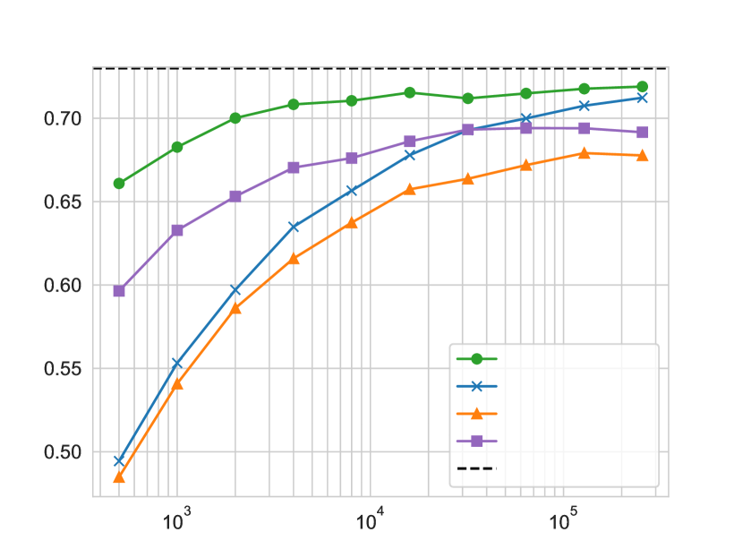
Figure 4: Test accuracy (higher the better) for a given power budget on Cifar-100 for different algorithms. The advantage of LASER is evident across the entire power spectrum.

Table 12: Power required (lower the better) to reach the given target accuracy on Cifar-100. LASER requires $16-32\times$ lesser power than the Z-SGD to achieve the same targetaccuracy. Equivalently, LASER tolerates more channel noise than the Z-SGD for the same target accuracy as is partly supported by our theoretical analysis.

Target	Power required		Reduction
	LASER	Z-SGD
$65\%$	$500$	$8000$	$16\times$
$68\%$	$1000$	$32000$	$32\times$
$70\%$	$2000$	$64000$	$32\times$
$71\%$	$8000$	$256000$	$32\times$

F.4 Mnist experimental setup

This section concerns the experimental details used to obtain Table 5 in the main text. Table 13 collects the settings we adopted to run our code.

Table 13: Default experimental settings for the 1-Layer NN used to learn the Mnist task.

Dataset	Mnist
Architecture	1-Layer NN
Number of workers	16
Batch size	$128$ per worker
Optimizer	SGD
Momentum	0.9
Learning rate	$0.01$
# Epochs	50
Weight decay	$1\text{\times}{10}^{-4}$,
Power budget	3 levels: $0.1,1,10$
Power allocation	Proportional to norm of compressed gradients (uncompressed gradients for Z-SGD)
Repetitions	3, with varying seeds
Compression	Rank 2 for LASER; $0.1$ compression factor for other baselines

F.5 Rank-accuracy tradeoff

There exists an inherent tradeoff between the decomposition rank $r$ (and hence the compression factor $\delta_{r}$) and the final model accuracy. In fact, a small rank $r$ implies aggressive compression and hence the compression noise dominates the channel noise. Similarly, for a high decomposition rank, the channel noise overpowers the compression noise as the power available per each coordinate is small. We empirically investigate this phenomenon for Cifar10 classification over various power regimes in Fig. 5.

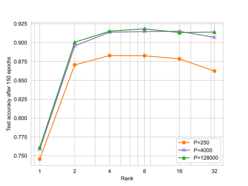
Figure 5: Final accuracy vs. compression rank tradeoff for CIFAR-10 classification, for low, medium and high power regimes. Rank-$4$/Rank-$8$ compression is optimal for all the three regimes. It reveals two interesting insights: (i) performance is uniformly worse in all the regimes with overly aggressive rank-one compression, and (ii) higher rank compression impacts low power regime more significantly than the medium and high-power counterparts. This confirms with the intuition that at low power (and hence noisier channel), it is better to allocate the limited power budget appropriately to few “essential” rank components as opposed to thinning it out over many.

As Fig. 5 reveals, either Rank-$4$ or Rank-$8$ compression is optimal for all the three power regimes. Further we observe two interesting trends: (i) the final accuracy is uniformly worse in all the regimes with overly aggressive rank-one compression, and (ii) higher rank compression impacts the low power regime more significantly than the medium and high-power counterparts. This is in agreement with the intuition that at low power (and hence noisier channel), it is better to allocate the limited power budget appropriately to few “essential” rank components as opposed to thinning it out over many. This phenomenon can be theoretically explained by characterizing the compression factor $\delta_{r}$ as a function of rank $r$ and its effect on the model convergence. While the precise expression for $\delta_{r}$ is technically challenging, given the inherent difficulty in analyzing the PowerSGD algorithm (Vogels et al., 2019), we believe that a tractable characterization of this quantity (via upper bounds etc.) can offer fruitful insights into the fundamental rank-accuracy tradeoff at play.

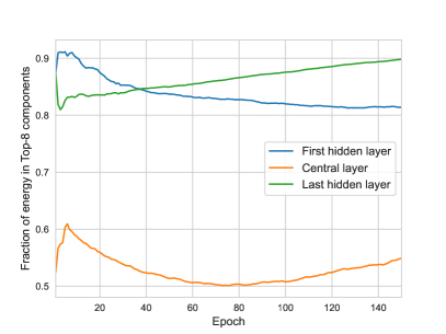
Figure 6: Fraction of energy in the top 8 components of the gradients of three layers in the network: the first and last hidden layer, and one central layer.

To further shed light on this phenomenon, we trained the noiseless SGD on Cifar10 and captured the evolution across the epochs of the energy contained in the top eight components of each gradient matrix. As illustrated in Fig. 6, we observe that for the first and last hidden layers, $80\%$ of the energy is already captured in these eight components. On the other hand, for the middle layer this fares around $55\%$. It is interesting to further explore this behavior for GPT models and other tasks.

F.6 Power allocation across workers and neural network parameters

The choice of power allocation over the layers of the network is perhaps the most important optimization required in our experimental setup. Notice that, because of Eq. (2), all clients must allocate the same power to a given gradient, since otherwise it would be impossible to recover the correct average gradient. However, workers have a degree of freedom in choosing how to distribute the power budget among gradients, i.e. among the layers of the network, and this power allocation can change over the iterations of the model training.

App. B.1 analyzes power allocation optimality from a theoretical point of view. On the experimental side, simpler schemes are enough to get significant gains over the other baselines. As a matter of fact, we considered the following power allocation scheme for the experiments: at each iteration, each worker determines locally how to allocate its power budget across the gradients. Then, we assume that this power allocation choice is communicated by the client to the server noiselessly. The server then takes the average of the power allocation choices, and communicates the final power allocation to the clients. The clients then use this power allocation to send the gradients to the server via the noisy channel.

For the determination of each worker’s power allocation, three schemes were considered:

• uniform power to each gradient;

• power proportional to the Frobenius norm (or the square of it) of the gradients;

• power proportional to the norm of the compressed gradients (i.e., the norm of what is actually communicated to the server).

For Z-SGD, where there is no gradient compression, the best power allocation turned out to be the one proportional to the norm of the gradients, independently of the power constraint imposed. For all the other algorithms, the best is power proportional to the norm of the compressed gradients.

F.7 Static vs. dynamic power policy

As discussed in Sec. 4.2, we analyzed different power allocation schemes across iterations, when a fixed budget in terms of average power over the epochs is given. Fig. 3 shows the results for decreasing power allocations, while Fig. 7 here shows their increasing counterparts. We observe that LASER exhibits similar gains over Z-SGD for all the power control laws. Further, constant power remains the best policy for both LASER and Z-SGD. Whilst matching the constant power performance, the power-decreasing control performs better than the increasing counterpart for Z-SGD, especially in the low-power regime, where the accuracy gains are roughly $4-5\%$.

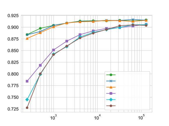
Figure 7: Final accuracy vs. power budget $P$ with various power control schemes, for distributed training across $16$ workers with ResNet18 on Cifar10. For each budget $P$, we consider three increasing power control laws, as studied in the literature [1], that satisfy the average power constraint: (i) constant power, $P_{t}=P$, (ii) piecewise constant, with the power levels $P_{t}\in\{P/3,2P/3,P,4P/3,5P/3\}$, and (iii) linear law between the levels $P/3$ and $5P/3$. The performance of increasing power allocation schemes is equal or worse compared to their decreasing counterparts of Fig. 3.

F.8 Baselines implementation

In this section we describe our implementation of the baselines considered in the paper.

F.8.1 Count-Mean Sketching

Algorithm 2 Count-Mean Sketching

compressgradient matrix $M\in\mathbb{R}^{n\times m}$Treat $M$as a vector of length $nm$. The number of samples $b$is set to $mn\times\text{(compression factor)}$. If the resulting $b$is less than 1, we set $b=1$. Sample a set of

References

• Aji & Heafield (2017) Aji, A. F. and Heafield, K. Sparse communication for distributed gradient descent. arXiv preprint arXiv:1704.05021, 2017.
• Alistarh et al. (2017) Alistarh, D., Grubic, D., Li, J., Tomioka, R., and Vojnovic, M. Qsgd: Communication-efficient sgd via gradient quantization and encoding. Advances in neural information processing systems, 30, 2017.
• Amiri & Gündüz (2020a) Amiri, M. M. and Gündüz, D. Federated learning over wireless fading channels. IEEE Transactions on Wireless Communications, 19(5):3546–3557, 2020a.
• Amiri & Gündüz (2020b) Amiri, M. M. and Gündüz, D. Machine learning at the wireless edge: Distributed stochastic gradient descent over-the-air. IEEE Transactions on Signal Processing, 68:2155–2169, 2020b.
• Basu et al. (2019) Basu, D., Data, D., Karakus, C., and Diggavi, S. Qsparse-local-sgd: Distributed sgd with quantization, sparsification and local computations. Advances in Neural Information Processing Systems, 32, 2019.
• Bernstein et al. (2018) Bernstein, J., Zhao, J., Azizzadenesheli, K., and Anandkumar, A. signsgd with majority vote is communication efficient and fault tolerant. arXiv preprint arXiv:1810.05291, 2018.
• Bottou et al. (2018) Bottou, L., Curtis, F. E., and Nocedal, J. Optimization methods for large-scale machine learning. SIAM review, 60(2):223–311, 2018.
• Chang & Tandon (2020) Chang, W.-T. and Tandon, R. Mac aware quantization for distributed gradient descent. In GLOBECOM 2020-2020 IEEE Global Communications Conference, pp.  1–6. IEEE, 2020.
• Cho et al. (2019) Cho, M., Muthusamy, V., Nemanich, B., and Puri, R. Gradzip: Gradient compression using alternating matrix factorization for large-scale deep learning. In NeurIPS. 2019.
• Cordonnier (2018) Cordonnier, J.-B. Convex optimization using sparsified stochastic gradient descent with memory. Technical report, 2018.
• Cover (1972) Cover, T. Broadcast channels. IEEE Transactions on Information Theory, 18(1):2–14, 1972. doi: 10.1109/TIT.1972.1054727.
• Dean et al. (2012) Dean, J., Corrado, G., Monga, R., Chen, K., Devin, M., Mao, M., Ranzato, M., Senior, A., Tucker, P., Yang, K., et al. Large scale distributed deep networks. Advances in neural information processing systems, 25, 2012.
• Dettmers (2015) Dettmers, T. 8-bit approximations for parallelism in deep learning. arXiv preprint arXiv:1511.04561, 2015.
• Dryden et al. (2016) Dryden, N., Moon, T., Jacobs, S. A., and Van Essen, B. Communication quantization for data-parallel training of deep neural networks. In 2016 2nd Workshop on Machine Learning in HPC Environments (MLHPC), pp.  1–8. IEEE, 2016.
• Guo et al. (2020) Guo, H., Liu, A., and Lau, V. K. Analog gradient aggregation for federated learning over wireless networks: Customized design and convergence analysis. IEEE Internet of Things Journal, 8(1):197–210, 2020.
• Haddadpour et al. (2020) Haddadpour, F., Karimi, B., Li, P., and Li, X. Fedsketch: Communication-efficient and private federated learning via sketching. CoRR, abs/2008.04975, 2020. URL https://arxiv.org/abs/2008.04975.
• Horvóth et al. (2022) Horvóth, S., Ho, C.-Y., Horvath, L., Sahu, A. N., Canini, M., and Richtárik, P. Natural compression for distributed deep learning. In Mathematical and Scientific Machine Learning, pp. 129–141. PMLR, 2022.
• Isik et al. (2022) Isik, B., Pase, F., Gunduz, D., Weissman, T., and Zorzi, M. Sparse random networks for communication-efficient federated learning. arXiv preprint arXiv:2209.15328, 2022.
• Ivkin et al. (2019) Ivkin, N., Rothchild, D., Ullah, E., Stoica, I., Arora, R., et al. Communication-efficient distributed sgd with sketching. Advances in Neural Information Processing Systems, 32, 2019.
• Jiang et al. (2018) Jiang, J., Fu, F., Yang, T., and Cui, B. Sketchml: Accelerating distributed machine learning with data sketches. In Proceedings of the 2018 International Conference on Management of Data, pp.  1269–1284, 2018.
• Karimireddy et al. (2019) Karimireddy, S. P., Rebjock, Q., Stich, S., and Jaggi, M. Error feedback fixes signsgd and other gradient compression schemes. In International Conference on Machine Learning, pp. 3252–3261. PMLR, 2019.
• Li et al. (2018) Li, Y., Park, J., Alian, M., Yuan, Y., Qu, Z., Pan, P., Wang, R., Schwing, A., Esmaeilzadeh, H., and Kim, N. S. A network-centric hardware/algorithm co-design to accelerate distributed training of deep neural networks. In 2018 51st Annual IEEE/ACM International Symposium on Microarchitecture (MICRO), pp.  175–188. IEEE, 2018.
• Lim et al. (2019) Lim, H., Andersen, D. G., and Kaminsky, M. 3lc: Lightweight and effective traffic compression for distributed machine learning. Proceedings of Machine Learning and Systems, 1:53–64, 2019.
• Martin & Mahoney (2021) Martin, C. H. and Mahoney, M. W. Implicit self-regularization in deep neural networks: Evidence from random matrix theory and implications for learning. The Journal of Machine Learning Research, 22(1):7479–7551, 2021.
• Mazumder et al. (2010) Mazumder, R., Hastie, T., and Tibshirani, R. Spectral regularization algorithms for learning large incomplete matrices. The Journal of Machine Learning Research, 11:2287–2322, 2010.
• Nazer & Gastpar (2007) Nazer, B. and Gastpar, M. Computation over multiple-access channels. IEEE Transactions on information theory, 53(10):3498–3516, 2007.
• Pagliardini (2023) Pagliardini, M. GPT-2 modular codebase implementation. https://github.com/epfml/llm-baselines, 2023.
• Ramesh et al. (2021) Ramesh, A., Pavlov, M., Goh, G., Gray, S., Voss, C., Radford, A., Chen, M., and Sutskever, I. Zero-shot text-to-image generation. In International Conference on Machine Learning, pp. 8821–8831. PMLR, 2021.
• Robbins & Monro (1951) Robbins, H. and Monro, S. A stochastic approximation method. The annals of mathematical statistics, pp.  400–407, 1951.
• Rothchild et al. (2020) Rothchild, D., Panda, A., Ullah, E., Ivkin, N., Stoica, I., Braverman, V., Gonzalez, J., and Arora, R. Fetchsgd: Communication-efficient federated learning with sketching. In International Conference on Machine Learning, pp. 8253–8265. PMLR, 2020.
• Saha et al. (2022) Saha, R., Rini, S., Rao, M., and Goldsmith, A. J. Decentralized optimization over noisy, rate-constrained networks: Achieving consensus by communicating differences. IEEE Journal on Selected Areas in Communications, 40(2):449–467, 2022. doi: 10.1109/JSAC.2021.3118428.
• Seide et al. (2014) Seide, F., Fu, H., Droppo, J., Li, G., and Yu, D. 1-bit stochastic gradient descent and its application to data-parallel distributed training of speech dnns. In Fifteenth annual conference of the international speech communication association, 2014.
• Shi et al. (2020) Shi, Y., Yang, K., Jiang, T., Zhang, J., and Letaief, K. B. Communication-efficient edge AI: Algorithms and systems. IEEE Communications Surveys & Tutorials, 22(4):2167–2191, 2020.
• Stewart & Miller (1975) Stewart, G. and Miller, J. Methods of simultaneous iteration for calculating eigenvectors of matrices. Topics in Numerical Analysis II, 2, 1975.
• Stich & Karimireddy (2019) Stich, S. U. and Karimireddy, S. P. The error-feedback framework: Better rates for SGD with delayed gradients and compressed communication. arXiv preprint arXiv:1909.05350, 2019.
• Stich & Karimireddy (2020) Stich, S. U. and Karimireddy, S. P. The error-feedback framework: Better rates for SGD with delayed gradients and compressed updates. The Journal of Machine Learning Research, 21(1):9613–9648, 2020.
• Stich et al. (2018) Stich, S. U., Cordonnier, J.-B., and Jaggi, M. Sparsified SGD with memory. Advances in Neural Information Processing Systems, 31, 2018.
• Sun et al. (2019) Sun, H., Shao, Y., Jiang, J., Cui, B., Lei, K., Xu, Y., and Wang, J. Sparse gradient compression for distributed sgd. In Database Systems for Advanced Applications: 24th International Conference, DASFAA 2019, Chiang Mai, Thailand, April 22–25, 2019, Proceedings, Part II, pp.  139–155. Springer, 2019.
• Tang et al. (2020) Tang, Z., Shi, S., Chu, X., Wang, W., and Li, B. Communication-efficient distributed deep learning: A comprehensive survey. arXiv preprint arXiv:2003.06307, 2020.
• Tsuzuku et al. (2018) Tsuzuku, Y., Imachi, H., and Akiba, T. Variance-based gradient compression for efficient distributed deep learning. arXiv preprint arXiv:1802.06058, 2018.
• Vargaftik et al. (2021) Vargaftik, S., Ben-Basat, R., Portnoy, A., Mendelson, G., Ben-Itzhak, Y., and Mitzenmacher, M. Drive: One-bit distributed mean estimation. Advances in Neural Information Processing Systems, 34:362–377, 2021.
• Vargaftik et al. (2022) Vargaftik, S., Basat, R. B., Portnoy, A., Mendelson, G., Itzhak, Y. B., and Mitzenmacher, M. Eden: Communication-efficient and robust distributed mean estimation for federated learning. In International Conference on Machine Learning, pp. 21984–22014. PMLR, 2022.
• Vogels et al. (2019) Vogels, T., Karimireddy, S. P., and Jaggi, M. PowerSGD: Practical low-rank gradient compression for distributed optimization. Advances in Neural Information Processing Systems, 32, 2019.
• Wang et al. (2018) Wang, H., Sievert, S., Liu, S., Charles, Z., Papailiopoulos, D., and Wright, S. Atomo: Communication-efficient learning via atomic sparsification. Advances in Neural Information Processing Systems, 31, 2018.
• Wangni et al. (2018) Wangni, J., Wang, J., Liu, J., and Zhang, T. Gradient sparsification for communication-efficient distributed optimization. Advances in Neural Information Processing Systems, 31, 2018.
• Wei & Shen (2022a) Wei, X. and Shen, C. Federated learning over noisy channels: Convergence analysis and design examples. IEEE Transactions on Cognitive Communications and Networking, 8(2):1253–1268, 2022a.
• Wei & Shen (2022b) Wei, X. and Shen, C. Federated learning over noisy channels: Convergence analysis and design examples. IEEE Transactions on Cognitive Communications and Networking, 8(2):1253–1268, 2022b.
• Wen et al. (2017) Wen, W., Xu, C., Yan, F., Wu, C., Wang, Y., Chen, Y., and Li, H. Terngrad: Ternary gradients to reduce communication in distributed deep learning. Advances in neural information processing systems, 30, 2017.
• Xu et al. (2020) Xu, H., Ho, C.-Y., Abdelmoniem, A. M., Dutta, A., Bergou, E. H., Karatsenidis, K., Canini, M., and Kalnis, P. Compressed communication for distributed deep learning: Survey and quantitative evaluation. Technical report, 2020.
• Yoshida & Miyato (2017) Yoshida, Y. and Miyato, T. Spectral norm regularization for improving the generalizability of deep learning. arXiv preprint arXiv:1705.10941, 2017.
• Yu et al. (2018) Yu, M., Lin, Z., Narra, K., Li, S., Li, Y., Kim, N. S., Schwing, A., Annavaram, M., and Avestimehr, S. Gradiveq: Vector quantization for bandwidth-efficient gradient aggregation in distributed cnn training. Advances in Neural Information Processing Systems, 31, 2018.
• Yu et al. (2019) Yu, Y., Wu, J., and Huang, J. Exploring fast and communication-efficient algorithms in large-scale distributed networks. arXiv preprint arXiv:1901.08924, 2019.
• Zhu et al. (2019) Zhu, G., Wang, Y., and Huang, K. Broadband analog aggregation for low-latency federated edge learning. IEEE Transactions on Wireless Communications, 19(1):491–506, 2019.