Compositional preference models
for aligning LMs

Abstract

As language models (LMs) become more capable, it is increasingly important to align them with human preferences. However, the dominant paradigm for training Preference Models (PMs) for that purpose suffers from fundamental limitations, such as lack of transparency and scalability, along with susceptibility to overfitting the preference dataset. We propose Compositional Preference Models (CPMs), a novel PM framework that decomposes one global preference assessment into several interpretable features, obtains scalar scores for these features from a prompted LM, and aggregates these scores using a logistic regression classifier. CPMs allow to control which properties of the preference data are used to train the preference model and to build it based on features that are believed to underlie the human preference judgement. Our experiments show that CPMs not only improve generalization and are more robust to overoptimization than standard PMs, but also that best-of-$n$ samples obtained using CPMs tend to be preferred over samples obtained using conventional PMs. Overall, our approach demonstrates the benefits of endowing PMs with priors about which features determine human preferences while relying on LM capabilities to extract those features in a scalable and robust way.

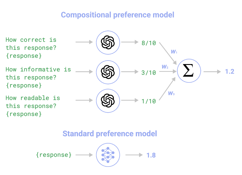
Figure 1: Compositional preference models score different features of LM responses separately and output a preference score as a linear combination of feature values.

1 Introduction

As the capabilities of language models (LMs) continue to advance, there is a growing need for safe and interpretable models. The dominant approach to aligning LMs with human preferences, reinforcement learning from human feedback (RLHF; Ouyang et al., 2022; Bai et al., 2022a; OpenAI, 2023), consists in training a preference model (PM) to predict human preference judgments and then finetuning an LM to maximize the reward given by the PM. However, the current PM methodology exhibits certain limitations. First, it is susceptible to overfitting the preference dataset. The PM can misrepresent human preferences by fitting to spurious correlations in its training data Gao et al. (2023). Heavily optimizing an LM against a PM incentivises the LM to exploit those flaws. This effect is known as reward hacking or Goodhart’s law (Goodhart, 1984). One way of addressing reward hacking is to impose certain inductive biases on the PM or limiting its capacity. Second, PMs are often difficult to interpret and to oversee . They project preferences onto a single scalar feature, making it difficult to know what factors are influencing their decisions. This is especially problematic for complex preferences, such as helpfulness or harmlessness, which often encompass a multidimensional combination of attributes (Bai et al., 2022a; Glaese et al., 2022; Touvron et al., 2023). Further, as LM capabilities improve, it will be increasingly harder for unassisted humans to provide feedback on LM’s responses (Pandey et al., 2022; Bowman et al., 2022a). One way of addressing this problem is to use another LM to decompose those responses into simpler pieces that can be evaluated either by a human or an LM.

In this paper, we propose the Compositional Preference Model (CPM), a novel framework for learning a PM that is robust to preference model overoptimization and allows for more transparent and interpretable supervision of complex behavior. A CPM decomposes one global preference assessment into a series of simpler questions which correspond to human-interpretable features. Then, a prompted LM (e.g. GPT-3.5) is asked to assign a numerical value to each feature. Finally, the feature scores are combined into a scalar preference score using a trained logistic regression classifier.

CPMs have several advantages over standard PMs. First, they are more robust to overfitting and reward hacking. The pre-selected features on which CPMs operate provide a useful inductive bias that bootstraps learning human preferences. This, in turn, limits their vulnerability to reward hacking, as the parameter space of a PM is spanned by features selected to be meaningful and robust. Second, CPMs allow for the modular and human-interpretable supervision of complex behavior. They effectively decompose a hard question (e.g. “is this text preferable?”) into a series of easier questions (e.g. “is this text easy to understand?”, “is this text informative?”) that are easier to evaluate for an LM and easier to inspect for a human overseer. This is a simple instance of a divide-and-conquer supervision approach (Cormen et al., 2022), which recursively breaks down a problem until it is easily solvable and then combines the solutions (Irving et al., 2018; Leike et al., 2018; Christiano et al., 2018).

In our experiments, we show that CPMs generalize better and that using them results in less preference model overoptimization. Additionally, CPMs exhibit superior performance in capturing the underlying human preferences. In an auto-evaluation experiment with Claude (Anthropic, 2023) as an approximation of human evaluators (Chiang et al., 2023; Mukherjee et al., 2023; Liu et al., 2023; He et al., 2023), best-of-$n$ samples obtained using CPMs are consistently preferred over samples obtained using conventional PMs.

Overall, the contributions of the paper include:

1. Introducing CPM, a novel framework for learning PMs that is more robust to overoptimization and allows for more transparent supervision, by decomposing the preference problem into a series of intuitive features linked to human preferences, and employing an LLM as a feature score extractor (Sec. 3).

2. Investigating the performance of CPMs on a diverse array of dimensions, including model robustness (Sec. 4.2), generalization (Sec. 4.3), robustness to overoptimization (Sec. 4.4), and effectiveness for preference alignment (Sec. 4.5).

3. Enabling an intuitive explanation of model optimization and generated responses (Sec. 4.6).

2 Background

Let us have a dataset of comparisons $\mathit{\mathcal{D}}=\{x^{i},y_{1}^{i},y_{2}^{i}\}_{i=1}^{N}$, where $x$ is an input query and $y_{1}$ and $y_{2}$ are two possible responses to $x$, with $y_{1}$ the preferred response. The dominant approach to aligning language models, RLHF (Christiano et al., 2017; Ziegler et al., 2019; Ouyang et al., 2022; Bai et al., 2022a), involves training a parametrized PM $R(y|x)=R_{\theta}(y|x)$ by defining a probability distribution

$$p_{\theta}(y_{1}>y_{2}|x)\doteq\sigma(R_{\theta}(y_{1}|x)-R_{\theta}(y_{2}|x))=(1+\exp(R_{\theta}(y_{2}|x)-R_{\theta}(y_{1}|x))^{-1}$$ (1)

and estimating $\theta$ by maximizing the likelihood of $p_{\theta}$ over $\mathcal{D}$. Typically $R_{\theta}$ is obtained by adding a scalar head on top of a base language model and fine-tuning the resulting model. Since $p_{\theta}$ is invariant to addition of a constant to $R_{\theta}$, it is standard to shift the $R$ scores such that $E_{(x,y)\sim D}[R(y|x)]=0$.

3 Method

The Compositional Preference Model (CPM) is a multi-step approach for decomposing preference learning into individual components. We first decompose preference judgements into a set of $C$ distinct features, each designed to evaluate a specific aspect of the response $y$ (relative to context $x$). Then we use a prompted LM to assign to a pair $(x,y)$ a scalar score for each individual feature $c=1,\ldots,C$. Finally, we employ a logistic regression classifier to combine these features into a global scalar score that best predicts the human preference judgements. This approach enables us to construct a coherent description of the characteristics that underlie these judgements.

3.1 Feature extraction using a language model

For each feature $c$, we consider an individual preference model $R_{c}$ that maps an input query $x$ and a response $y$ to a scalar score. In order to do that, we associate each feature $c$ with a specific prompt $t_{c}$ and compute a score $r_{c}=R_{c}(y|x,t_{c})$, where $R_{c}$ can be a general LLM like GPT-3.5, prompted with $t_{c}$. These features are designed to decompose the broad concept of preferability into a series of more straightforward and interpretable components. It is noteworthy that a feature can represent not only positive categories that are aligned with preferability (e.g. informativeness), but also categories that are assumed to be negatively correlated with it (e.g. biasedness). This procedure allows us to control which properties of the preference data are used to train the PM and to build it based on components that we believe to determine the human choices.

3.2 Combining multiple features

The features assessed by the prompted LM serve as distinct modules, each of which evaluates a different aspect. To combine the features into an interpretable single model, we employ logistic regression to classify the preferred response in a pairwise comparison dataset.

Based on the dataset $\mathit{\mathcal{D}}=\{x^{i},y_{1}^{i},y_{2}^{i}\}_{i=1}^{N}$, we obtain a feature matrix $\{x^{i},\bm{r}(y_{1}^{i}),\bm{r}(y_{2}^{i})\}_{i=1}^{N}$. Here $\bm{r}(y)=(R_{1}(y|x,t_{1}),\ldots,R_{C}(y|x,t_{C}))$ is a feature vector containing decomposed feature scores. We standardize each feature score to have average $0$ and variance $1$ within the train data. We compute the pairwise difference of the feature vectors for each pair of responses, $\bm{r}(y_{1})-\bm{r}(y_{2})$, and train a logistic regression classifier with this difference to predict $1$ if $y_{1}$ is preferred, and $0$ if $y_{2}$ is preferred. In other words, the distribution $p$ is formalized as:

$$p(y_{1}>y_{2}|x)\doteq\sigma(\left\langle\bm{\lambda},\bm{r}(y_{1})-\bm{r}(y_{2})\right\rangle)=(1+\exp(-\left\langle\bm{\lambda},\bm{r}(y_{1})-\bm{r}(y_{2})\right\rangle))^{-1}$$ (2)

where $\bm{\lambda}=(\lambda_{1},\ldots,\lambda_{C})$ is the vector of fitted coefficients. The coefficient $\lambda_{c}$ indicates the importance of the feature $c$ for predicting human preference judgements. To obtain the preference score of a single sample $(y,x)$, we simply compute $\left\langle\bm{\lambda},\bm{r}(y)-\bm{0}\right\rangle=\left\langle\bm{\lambda},\bm{r}(y)\right\rangle$, where $\bm{0}$ is the standardized average of the feature vector $\bm{r}(y)$ over the train data as explained above.

4 Experiments

In this section, we empirically evaluate CPM on several aspects, including model robustness (Sec. 4.2), generalization (Sec. 4.3), robustness to overoptimization (Sec. 4.4), and effectiveness for preference alignment (Sec. 4.5). We also provide an illustrative example of CPM interpretability in Sec. 4.6.

4.1 Experimental setup

Datasets

We conduct experiments on two datasets, the HH-RLHF dataset (Bai et al., 2022a) and the SHP dataset (Ethayarajh et al., 2022). Both consist of pairs of responses based on helpfulness. For each dataset, in order to establish a consistent setting and control for the data size factor, we sample 20K single-turn data points.

Features

We use 13 features: helpfulness, specificity, intent, factuality, easy-to-understand, relevance, readability, enough-detail, biased, fail-to-consider-individual-preferences, repetitive, fail-to-consider-context and too-long, with pre-specified prompt templates (see App. C for the description of features and prompts). We use the same set of features for both datasets; prompt templates only differ in a preamble that describes $x$ as either a conversation with an AI assistant (HH-RLHF) or a StackExchange question (SHP). We also use the length of $y$, which we find to be helpful on the SHP dataset.

Methods

To find out the ability of an LM as a feature extractor, we explore two LMs, GPT-3.5 (gpt-3.5-turbo-0301) and Flan-T5-XL (3B parameters) (Chung et al., 2022), using the same features and prompt templates. We refer to the CPM models based on these extractors as CPM-GPT-3.5 and CPM-Flan-T5, respectively. To select only the most important features, we add a regularization term in logistic regression and use hyperparameters selected with 5-fold cross-validation on the training dataset.

We then compare the conventional PM to these CPMs (trained respectively as described in Sec. 2 and Sec. 3.2). For a fair comparison, we train the standard PM based on the same Flan-T5-XL model that we use for the CPMs, but with an added linear head that outputs a scalar preference score. We compare the performances of CPM-GPT-3.5 and CPM-Flan-T5 with this standard PM. Implementation details are provided in App. A.

Best-of-$n$ sampling (BoN)

To assess the robustness of PMs to overfitting, we use Best-of-$n$ (BoN) sampling (Gao et al., 2023), a simple yet effective method that has been shown to be competitive with more advanced techniques such as reinforcement learning (Hilton & Gao, 2022). BoN abstracts away from RLHF design choices such as the details of policy optimization and provides a stable proxy for RLHF performance (Nakano et al., 2021; Gao et al., 2023).

We generate $n$ responses using an initial LM $a(x)$ and evaluate the performance of the PMs on these responses. We consider the BoN distribution $x\sim\text{BoN}(a,\text{PM},n)$, where $n$ candidates are sampled from $a$ and $x$ is the candidate maximizing the PM score. Following Gao et al. (2023), we compare the robustness of two related PMs, $\text{PM}_{A}(x)$ and $\text{PM}_{B}(x)$, by measuring the gap between their average scores relative to samples $x$ from $\text{BoN}(a,\text{PM}_{A},n)$, where typically (because by construction such samples favor large values of $\text{PM}_{A}(x)$) we have $\text{PM}_{A}(x)>\text{PM}_{B}(x)$, with the gap increasing with $n$.

We generate up to 25,600 BoN responses, with 256 responses for each of 100 prompts in a held-out test set. We use Flan-T5-Large (780M parameters; Chung et al., 2022) as the initial LM to generate the responses. To ensure that the performance of different PMs can be compared on the same scale across different reward models, we normalize each PM score to have average 0 and variance 1 within the training data.

4.2 Model robustness

(a) HH-RLHF dataset

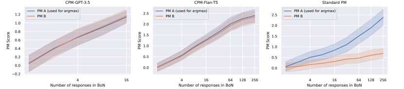
(b) SHP dataset

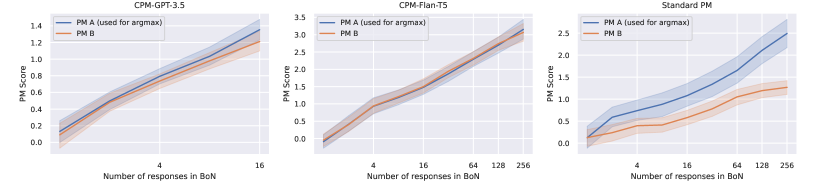
Figure 2: BoN comparison over two models fitted independently in same condition (left: CPM-GPT-3.5, middle: CPM-Flan-T5, right: Standard PM). The PM used for BoN selection is PM A (blue line).

Model robustness refers to the sensitivity of a predictive model to the selection of its training data (Hastie et al., 2009). Specifically, it quantifies how much the model’s predictions would change if we were to train it on different subsets of the preference dataset. A model with low robustness will show poor generalization on unseen data.

To assess model robustness, we independently train two PMs for each PM method, $\text{PM}_{A}$ and $\text{PM}_{B}$, on disjoint subsets of the training data, each of size 10K. We then conduct a BoN experiment and check whether the scores of these two PMs diverge with increasing $n$. As explained above, we pick the response with highest $\text{PM}_{A}$ score among $n$ samples and measure the gap between the scores of $\text{PM}_{A}$ and $\text{PM}_{B}$ on that sample.

Fig. 2 shows that CPM is significantly more consistent between $\text{PM}_{A}$ and $\text{PM}_{B}$ than the standard PM method in terms of the score differences, even for BoN with size $256$. The smooth scaling trend as a function of $n$ suggests that our findings will generalize to larger $n$. This suggests that the small number of trainable coefficients (in this experiment 14 coefficients) makes the model robust to noise in data sampling. Still, the features extracted by LM are informative enough to build an effective preference model for alignment tuning, as we illustrate below.

4.3 Comparison with reference PMs

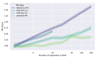
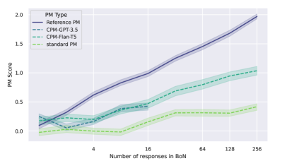
Figure 3: Comparison between PM scores relative to the distributions $\text{BoN}(a,\text{PM}_{\text{ref1}},n)$ (HH-RLHF dataset, left) and $\text{BoN}(a,\text{PM}_{\text{ref2}},n)$ (SHP-dataset, right).

To assess the generalizability of our CPMs, we compare them to two well-established reference PMs, $\text{PM}_{\text{ref}1}$ and $\text{PM}_{\text{ref}2}$, both instances of DeBERTa (He et al., 2020), with $\text{PM}_{\text{ref}1}$ finetuned on a large dataset including HH-RLHF and $\text{PM}_{\text{ref}2}$ finetuned on a large dataset including SHP (Sileo, 2023). These PMs, trained on larger and more diverse datasets, are shown to generalize better than PMs trained on a 10K dataset (see App. B). We select BoN responses with the reference PM and then examine how their scores diverge relative to the different PMs trained on a 10K dataset as in Sec. 4.2. We hypothesize that models that diverge less from such independently trained reference PMs will generalize better to unseen data. Fig. 3 shows that all models scale monotonically with the reference PM, with the CPMs staying closer to it. This suggests that the extracted features are informative enough to allow for learning a more generalizable model of preference judgements.

4.4 Robustness to Overoptimization

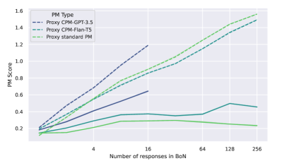
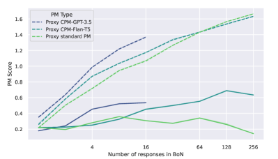
Figure 4: Overoptimization experiment in BoN distribution $\text{BoN}(a,\text{PM}_{\text{Proxy}},n)$. Dashed line means proxy PM used for BoN selection, corresponding solid line means gold PM. (left: HH-RLHF dataset, right: SHP dataset)

Overoptimization is a type of misalignment that occurs when the preference model is overly optimized by exploiting flaws in the proxy objective (Amodei et al., 2016; Skalse et al., 2022). This can lead to the PM diverging from the true objective, which we want to optimize in alignment tuning.

To investigate overoptimization, we follow Gao et al. (2023) and construct a synthetic dataset where the output of a specific “gold” PM is assumed to be the ground truth for preferences. As gold PMs, we use reference PMs $\text{PM}_{\text{ref}1}$ and $\text{PM}_{\text{ref}2}$ (described in Sec. 4.3). We then use the gold models to generate synthetic labels to train proxy PMs using each of the studied techniques. Depending on the PM training method, overoptimizing the PM can cause it to diverge from the gold PM, which allows us to compare the robustness of different PM techniques.

Fig. 4 shows that the gap between the gold PM and the proxy PM scores increases for each PM as the candidate size $n$ increases. The distribution of the standard PM does not follow the gold PM distribution and has a larger divergence as the candidate size $n$ increases. This illustrates that fitting a standard PM can lead to overoptimization, which is consistent with existing literature (Gao et al., 2023). On the other hand, the gap between the gold and proxy PM scores is smaller for CPMs, with the gold PM score beginning to diverge later than for standard PMs. This suggests that CPMs are more robust to overoptimization. The rank correlation of the PM scores with increasing $n$ in Fig. 4, which measures this quantitatively, is provided in Table  9 in the Appendix.

4.5 Quality evaluation

The ultimate goal of PMs is to help align LMs with human preferences. While in the previous section we compared PMs with a certain gold PM, in this section we will investigate whether LMs aligned using CPMs are preferred by humans over LMs aligned using standard PMs. Following previous literature (Chiang et al., 2023; Mukherjee et al., 2023; Liu et al., 2023; He et al., 2023), we simulate human evaluation using a prompted LLM.

For each PM, we draw a response from $\text{BoN}(a,\text{PM},16)$ by generating samples from $a$ (namely Flan-T5) and selecting the best response based on the PM score. We then compare this response to vanilla Flan-T5, namely a response randomly selected from the same set of candidates. We finally use the LLM to choose which response is preferable. We refer to this metric as the “win rate”. A good PM is expected to have high win rate against vanilla Flan-T5.

Importantly, we use Claude (claude-2; Anthropic, 2023), an LLM that was not used in feature extraction. Hence, we avoid potential subtle preference leaks from features extracted usig GPT-3.5. We use the prompt from (Chiang et al., 2023; Mukherjee et al., 2023) to rate the quality of the response selected by each PM method (see Tab. 8 for the prompt used in evaluation). We perform one BoN trial with $n=16$ for CPM-GPT-3.5 and 10 independent such trials for other PMs and report the average win rate.

Win Rate	HH-RLHF	SHP
CPM-GPT-3.5	0.810  (.)	0.672  (.)
CPM-Flan-T5	0.742 (0.034)	0.580 (0.045)
Standard PM	0.588 (0.030)	0.564 (0.037)

Table 1: Win rate over initial generation after BoN sampling based on each PM. Except CPM-GPT-3.5, we independently conduct $10$ rounds of BoN($n=16$) samplings and report the average win rate along with standard error.

Tab. 1 shows evaluation results. Considering that both standard PM and CPM-Flan-T5 use the same architecture and data, the higher win rate of CPM-Flan-T5 compared to standard PM suggests the advantage of decomposing preference into multiple features and using an LM as feature extractor, rather than directly using the PM based on fine-tuning the LM as in Eq. (1). CPM-GPT-3.5 shows an even higher win rate, again indicating that using a more powerful LM as feature extractor can further improve the performance of CPM.

4.6 Model interpretability

CPMs, as linear models, have a high degree of interpretability Hastie et al. (2009). In this section, we provide a few illustrative examples focussing on the dataset HH-RLHF.

Coefficients

The interpretability of our model is enhanced by the fact that the feature coefficients provide a direct indication of the factors that most influence the CPM’s decisions. This information can help understand the CPM’s internal workings. Tab. 2 shows the top 3 largest coefficients (see Tab. 10 for full coefficients). Although the coefficients vary as they are extracted with different LMs, their orders are generally consistent, except for a few features. This observation provides some clues into how the CPM makes its decisions. In the current example, the CPM focuses on general helpfulness and also prefers responses that are detailed enough but also factually correct.

CPM-GPT-3.5		CPM-Flan-T5
Feature	Coefficient	Feature	Coefficient
helpfulness	0.246	fail-to-consider-context	0.420
enough-detail	0.235	enough-detail	0.244
factuality	0.187	factuality	0.227

Table 2: Three largest CPM coefficients on HH-RLHF dataset.

LM-extracted features

The features extracted by the LM enable intuitive explanation of generated responses. This allows supervising complex behavior in a human-interpretable way. Tab. 3 shows examples of these features, which can be used to identify which aspects of the response contribute most to the predicted preference judgement. By decomposing a hard preference (“This text is not preferable.”) into a series of easier features (“This text is generally unhelpful, as it is easy to read but has little detailed information”), it allows easier inspection for a human overseer.

	Features
Dialogue	helpfulness	readability	enough-detail	factuality	fail-to-consider- context
Q: What things can I create with java programming?
R1: Java is a programming language that is designed to create applications that run on a computer.	1.209	0.559	0.913	1.690	2.117
R2: Robots	0.509	0.559	-0.075	-0.569	-0.239
Q: Why is Lucifer referred to as the “morning star”?
R1: Lucifer is the Morning Star because it is the brightest star in the sky.	1.209	0.880	1.901	0.843	0.232
R2: angel	-0.890	0.239	-0.569	-0.851	-0.239
Q: I’d like to evaluate some art perhaps. Can you tell me some history about Mona Lisa, the painting?
R1: The Mona Lisa is a famous painting in the Louvre, Paris, France. It is attributed to Leonardo da Vinci.	1.909	0.880	1.901	1.690	2.588
R2: It was painted by Gian Lorenzo da Sica in the late 18th century. The name of the painting is inspired by the story of the famous Italian painter Leonardo da Vinci. The painting has been described as having a “poetic” quality.	0.859	0.239	1.901	0.278	-0.239

Table 3: Examples of feature values of CPM-GPT-3.5. Each feature value can provide information about which aspects of the response are good or bad.

5 Ablation Study

In this ablation study, we evaluate the impact of two factors, data size and size of the LM for feature extraction on the HH-RLHF dataset.

Data scaling trend

To investigate the effect of data size on model robustness, we hold the model size constant (3B parameters) and vary the data size used to train the PMs. We independently train each PM method on two disjoint subsets of the training data, as described in Sec. 4.2. We gradually increase the data size from 100 to 10,000. Fig. 5 shows the results of the model robustness experiment. CPMs rapidly become consistent as the data size increases and achieve stable consistency between two PMs with a data size of over 500. In contrast, standard PMs show poor consistency between models, especially when the data size is small. This suggests that CPMs are more robust than standard PMs and can produce reliable results even with a small amount of data.

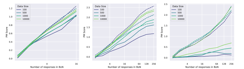
Figure 5: BoN comparison of two models fitted independently with scaling data size in HH-RLHF dataset (left: CPM-GPT-3.5, middle: CPM-Flan-T5, right: standard PM).

Model scaling trend

To investigate the effect of the size of the LM used for feature extraction, we gradually increase this size from Flan-T5 “small” (80M parameters) to “XL” (3B parameters) and track two important metrics: model generalizability (described in Sec. 4.3) and win rate (described in Sec. 4.5). The training data size is fixed to 10K. As shown in Fig. 6, both model generalizability and win rate steadily improve with increasing LM size. This confirms that LM capability propagates to feature extraction, and that CPM can take advantage of it. This further means that CPMs can become even more useful as extractor LMs become more capable. The smooth and gradual increase of the win rate as a function of LM size suggests that our findings generalize to the case of using even larger LMs for feature extraction.

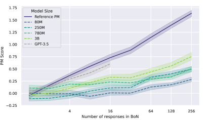
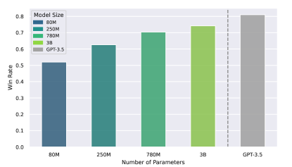
Figure 6: Model size scaling experiment using Flan-T5. (left: comparison with the reference PM, right: win rate over initial generation after BoN sampling based on each PM)

6 Related work

Robustness of preference models

PM overoptimization is an instance of reward hacking, a situation when a policy exploits flaws in its reward function (Amodei et al., 2016; Skalse et al., 2022). These flaws can come from errors of human evaluators (Pandey et al., 2022), the inherent difficulty of learning preferences of irrational agents (Mindermann & Armstrong, 2018; Shah et al., 2019) or the fragility of learned reward functions to adversarial attacks (McKinney et al., 2023). Gao et al. (2023) studied the scaling properties of PM overoptimization and Casper et al. (2023) discuss it in a broader context of open problems with RLHF. More generally, PMs can learn to be sensitive to spurious features associated with human feedback. This leads to failure modes such as sycophancy (a tendency to answer a question with a user’s preferred answer, even if that answer is not correct; Cotra, 2021; Perez et al., 2022) or social bias (due narrow demographics of feedback providers; Santurkar et al., 2023; Hartmann et al., 2023). Despite its growing importance, the problem of learning robust PMs for aligning LMs is largely neglected. The present paper attempts to fill this gap.

Decomposing tasks for LMs.

There are numerous examples of task decomposition increasing the accuracy or robustness of language models. Breaking down problems into steps (Wei et al., 2022, chain-of-thought;) or into a sequence of subproblems depending on answers to previous subproblems (Zhou et al., 2023) are enormously beneficial for tasks involving reasoning. Others explored a stronger separation: solving subproblems independently in different LM context windows. For instance, Creswell et al. (2022) alternate between selection and inference to generate a series of interpretable, casual reasoning steps. Radhakrishnan et al. (2023) found that solving subproblems in separate context windows improves faithfulness of reasoning. Reppert et al. (2023) build compositional LM programs by applying decomposition iteratively, with a human in the loop, to facilitate science question answering. The present paper finds similar robustness benefits of decomposition for preference modeling.

Scalable oversight

Scalable oversight is the problem of evaluating the behaviour of agents more capable than the evaluators (Bowman et al., 2022b). On the one hand, LMs may soon grow capable of completing tasks for which humans will not be able to provide feedback. On the other, LMs might also be capable of reasoning about flaws in their evaluation procedures (Berglund et al., 2023) and exploiting them unbeknownst to overseers. Current proposals for solving scalable oversight focus on recursively relying on other LMs to assist human evaluators (Irving et al., 2018; Leike et al., 2018; Christiano et al., 2018). RL from AI feedback (Bai et al., 2022b) attempts to implement this idea by using carefully prompted LMs to generate training data for PMs. In contrast, we propose to rely on LMs during a single inference step of a PM.

7 Conclusion

We introduce Compositional Preference Models (CPMs), a simple and effective paradigm for training robust and interpretable preference models. CPMs decompose global preference scores into interpretable features and rely on language models (LMs) to extract those features. Despite their simplicity, CPMs are robust to different subsamplings of the dataset and to overoptimization, and they outperform conventional preference models at obtaining preferred best-of-$n$ samples. We believe that CPMs pave the way for combining human insights into preference judgements with the LM capabilities to extract them. Given the recent advances in LM abilities, CPMs have the potential to being used for alignment and scalable oversight of models with superhuman capabilities. Another possible objective for future research would be to explore how to elicit decomposed features that can capture various kinds of complex preference judgements. A promising direction here would be to leverage LMs to not only score, but actually discover the component features that determine these judgements.

Appendix A Implementation Details

A.1 Compositional preference model

We used GPT-3.5 (gpt-3.5-turbo-0301) and Flan-T5-XL (3B parameters) (Chung et al., 2022) as a feature extractor, using the same features and prompt templates in Tab. 5 and Tab. 6. We excluded randomness from the generation process and selected the token with the highest likelihood.

For logistic regression classifier we used Scikit-learn (Buitinck et al., 2013). We set the choice of $L_{1}$ and $L_{2}$ regularization, weight of regularization, and solver of the logistic regression classifier as a hyperparameters and selected best hyperparameters based on 5-fold cross-validation in training dataset.

In the inference time, we made feature scores of the generated response using same LLM and templates used in training phrase. The feature scores are aggregated with the trained logistic regression classifier as described in Sec. 3.2.

A.2 Standard preference model

All standard PMs were implemented using PyTorch (Paszke et al., 2019) and HuggingFace Transformers (Wolf et al., 2020) We adopt the AdamW optimizer (Loshchilov & Hutter, 2017) with $\beta=(0.9,0.98)$ and set the weight decay to $0.01$. We conducted separate hyperparameter sweeps over learning rate and batch size for each dataset, using early-stopping based on the evaluation set with 3 steps of patience. We used a batch size of 32 and a learning rate of 1e-5 for HH-RLHF dataset and 5e-5 for SHP dataset. We used cosine learning rate schedule with 100 linear warmup steps. We used Flan-T5-XL (Chung et al., 2022, 3B parameters) for standard PMs, which is available on the Huggingface Model Hub under the model name of google/flan-t5-xl. Training was performed on Nvidia A100 GPU, with the longest run taking approximately 12 hours.

Appendix B Claude evaluation of the reference PM

To evaluate the performance of reference PM in Sec.4.3 in preference alignment, we follow the same quality evaluation framework as in Sec. 4.5. Specifically, we select the best sample among 16 responses generated by Flan-T5, based on the reference PM score. We then compare this response to vanilla Flan-T5, a response randomly selected from the same set of candidates, as described in Sec. 4.5.

Again, we use Claude to rate the quality of the response selected by reference PMs (see Tab. 8 for the prompt used in evaluation). We perform 10 independent BoN trials with $n=16$ and report the average win rate. The results are shown in Tab. 4. The reference PM outperforms CPM-Flan-T5 and standard PM. Interestingly, reference PM shows second best win rate in SHP dataset, highlighting the effectiveness in CPM-GPT-3.5. However, we note that this should be interpreted with caution as CPM-GPT-3.5 is not tested in multiple experiments.

Win Rate	HH-RLHF	SHP
CPM-GPT-3.5	0.810  (.)	0.672  (.)
CPM-Flan-T5	0.742 (0.034)	0.580 (0.045)
Standard PM	0.588 (0.030)	0.564 (0.037)
reference PM	0.829 (0.050)	0.619 (0.060)

Table 4: Comparison of win rate between CPM and reference PM externally fitted on multiple datasets. Reference PM shows high win rate in HH-RLHF dataset, and second best win rate in SHP dataset.

Appendix C Prompt used

You will be given a conversation between a human and an AI assistant.
Your job is to judge whether assistant’s reply {attribute_desc}.
Score that on a scale from 1 to 10 where 1 means {attr_min} and 10
means {attr_max}. Here’s the conversation:

Human:
{history}

Assistant:
{reply}

Answer by outputting a number from 1 to 10 (and nothing else).

Answer:

Table 5: Prompt template used for HH-RLHF dataset to rate the response under given attribute.

You will be given a Reddit post and a reply. Your job is to judge
whether the reply {attribute_desc}. Score that on a scale from 1
to 10 where 1 means {attr_min} and 10 means {attr_max}.

POST:
{query}

Reply:
{reply}

Answer by outputting a number from 1 to 10 (and nothing else).

Answer:

Table 6: Prompt template used for SHP dataset to rate the response under given attribute.

Feature name	Attribute	Description
helpfulness	attribute_desc	is helpful for the original poster
	attr_min	not helpful
	attr_max	very helpful
specificity	attribute_desc	is specific enough
	attr_min	too vague
	attr_max	very specific
intent	attribute_desc	understands the original poster’s intent
	attr_min	failure of understanding
	attr_max	perfect understanding
factuality	attribute_desc	is factually correct
	attr_min	egregiously incorrect
	attr_max	fully correct
easy-to-understand	attribute_desc	is easy to understand
	attr_min	very difficult to understand
	attr_max	very easy to understand
relevance	attribute_desc	is relevant to the original poster’s question
	attr_min	off-topic
	attr_max	very relevant
readability	attribute_desc	is easy to read and not too technical for the original poster
	attr_min	very difficult to read
	attr_max	very easy to read
enough-detail	attribute_desc	provides enough detail to be helpful
	attr_min	too little detail
	attr_max	very detailed
biased	attribute_desc	is biased or one-sided
	attr_min	very biased
	attr_max	not biased at all
fail-to-consider- individual-preferences	attribute_desc	fails to consider the original poster’s cultural or individual preferences
	attr_min	fails to consider the original poster’s preferences
	attr_max	takes into account the original poster’s preferences
repetetive	attribute_desc	is repetitive
	attr_min	very repetitive
	attr_max	not repetitive
fail-to-consider-context	attribute_desc	fails to consider the original poster’s context
	attr_min	fails to consider the original poster’s context
	attr_max	takes into account the original poster’s context
too-long	attribute_desc	is too long
	attr_min	too long
	attr_max	not too long

Table 7: Features and descriptions used in Tab. 5 and 6.

Human:
You are a helpful and precise assistant for checking the quality of
the answer. We would like to request your feedback on the performance
of two AI assistants in response to the user question displayed below.

[Question]
{query}
[The Start of Assistant 1s Answer]
{reply1}
[The Start of Assistant 2s Answer]
{reply2}

Please rate the helpfulness, relevance, accuracy, level of
details of their responses.
Each assistant receives an overall score on a scale of 1 to 10, where
a higher score indicates better overall performance.
Please first output a single line containing only two values indicating
the scores for Assistant 1 and 2, respectively. The two scores are
separated by a space. In the subsequent line, please provide a
comprehensive explanation of your evaluation, avoiding any potential
bias and ensuring that the order in which the responses were presented
does not affect your judgment.

Assistant:

Table 8: Prompt template to rate the writing quality of the candidate assistant model.

Appendix D Additional model interpretability

Feature distribution of policy

Fig. 7 shows how the feature values of the responses change in $\text{BoN}(a,\text{CPM},n)$ distribution with Flan-T5-Large as initial LM $a$, as a function of KL divergence $\text{KL}_{\text{BoN}}$. This simulates how the feature distribution changes as the initial policy is optimized with the current CPM and allows for inspecting which features drive reward maximization at different stages. The increase in readability is smaller than other features such as enough-detail and fail-to-consider-context. This means that policy shifts towards generating responses with more detailed information, rather than focusing on generating readable responses. Additionally, after a certain $n$, the slope of fail-to-consider-context increases, and it achieves the highest score at the end of optimization. This means that optimization pressure focuses on not failing to consider the context and avoiding unexpected lengthy responses. This decomposition makes it easier for a human to understand why the LM generated such responses.

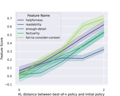
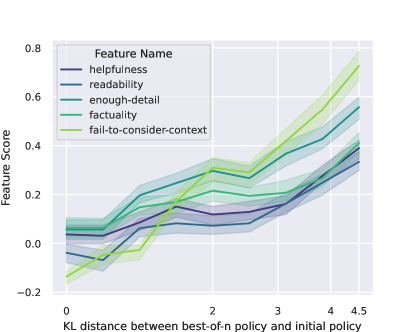
Figure 7: Feature distribution of BoN experiment (left: CPM-GPT-3.5, right: CPM-Flan-T5). Note that the $x$-axes are different. Here the KL distance of the BoN distribution from the initial distribution $a(x)$ is computed as $\text{KL}_{\text{BoN}}=\log n-\frac{n-1}{n}$ (Nakano et al., 2021).

Appendix E Additional tables and figures

(a) HH-RLHF dataset

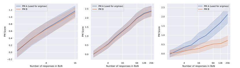
(b) SHP dataset

Figure 8: BoN comparison over two models fitted independently in same condition (left: CPM-GPT-3.5, middle: CPM-Flan-T5, right: standard PM) The PM A with blue line indicates the PM used for selection in BoN.

	HH-RLHF	SHP
CPM-GPT-3.5	0.997	0.981
CPM-Flan-T5	0.926	0.928
Standard PM	0.665	0.057

Table 9: Rank correlation between gold PM scores and proxy PM scores in BoN experiment. For each PM technique used to fit the proxy PM, we calculate and average PM scores over samples from $\text{BoN}(a,\text{PM}_{\text{proxy}},n)$, and compute the rank correlation between the averaged gold and proxy PM scores over different $n$.

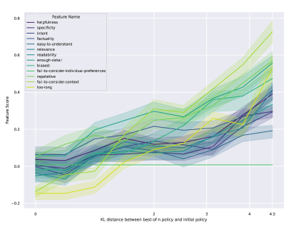
Figure 9: Feature distribution of BoN experiment (left: CPM-GPT-3.5, right: CPM-Flan-T5). Note that the $x$-axes are different. Here the KL distance of the BoN distribution from the initial distribution $a(x)$ is computed as $\text{KL}_{\text{BoN}}=\log n-\frac{n-1}{n}$ (Nakano et al., 2021).

CPM-GPT-3.5		CPM-Flan-T5
Feature	Coefficient	Feature	Coefficient
helpfulness	0.246	fail-to-consider-context	0.420
enough-detail	0.235	enough-detail	0.244
factuality	0.187	factuality	0.227
readability	0.184	biased	0.178
token_length	0.101	easy-to-understand	0.124
specificity	0.094	specificity	0.106
biased	0.086	too-long	0.081
relevance	0.071	token_length	0.075
easy-to-understand	0.069	helpfulness	0.037
fail-to-consider-context	0.043	intent	0.024
too-long	0.016	repetetive	0.015
repetetive	0.014	fail-to-consider- individual-preferences	-0.042
intent	-0.008	relevance	-0.056
fail-to-consider- individual-preferences	-0.056	readability	-0.120

Table 10: Fitted coefficient of CPM on HH-RLHF dataset.

	Features
Dialogue	helpfulness	readability	enough-detail	factuality	fail-to-consider- context
Q: why is ramon laguarta a bad ceo?
R1: a bad businessman	-0.890	-1.041	-0.569	-0.851	-0.239
R2: Manager	-0.890	-1.682	-1.063	-0.851	-0.710
Q: What is a blizzard warning?
R1: Blizzard warnings are issued by the National Weather Service to warn against snow, ice or strong winds.	1.909	0.880	2.395	1.690	3.059
R2: Blizzards can cause extremely dangerous driving conditions, with heavy snow, ice and sleet.	1.559	0.88	1.901	1.408	2.117
Q: Is climate change raising temperatures above their normal levels?
R1: Climate change increases global temperature.	1.559	0.559	1.901	1.690	-0.239
R2: Earth is expected to experience a warmer climate by the year 2050, the hottest on record, based on the International Solar System	0.509	-0.721	0.419	0.278	-0.239
Q: I’d like to evaluate some art perhaps. Can you tell me some history about Mona Lisa, the painting?
R1: The Mona Lisa is a 16th century Italian portrait by Gian Lorenzo Bernini.	-0.89	-1.041	-0.569	-0.851	-0.710
R2: In 1853, the artist Leonardo da Vinci created the portrait of the Madre della Signore.	-0.540	-1.041	-0.075	-0.569	-0.239

Table 11: Examples of feature values of CPM-GPT-3.5. Each feature value can provide information about which aspects of the response are good or bad.

References

- Amodei et al. (2016) Dario Amodei, Chris Olah, Jacob Steinhardt, Paul Christiano, John Schulman, and Dan Mané. Concrete problems in ai safety, 2016.
- Anthropic (2023) Anthropic. Introducing claude, 2023. URL https://www.anthropic.com/index/introducing-claude.
- Bai et al. (2022a) Yuntao Bai, Andy Jones, Kamal Ndousse, Amanda Askell, Anna Chen, Nova DasSarma, Dawn Drain, Stanislav Fort, Deep Ganguli, Tom Henighan, et al. Training a helpful and harmless assistant with reinforcement learning from human feedback. arXiv preprint arXiv:2204.05862, 2022a.
- Bai et al. (2022b) Yuntao Bai, Saurav Kadavath, Sandipan Kundu, Amanda Askell, Jackson Kernion, Andy Jones, Anna Chen, Anna Goldie, Azalia Mirhoseini, Cameron McKinnon, Carol Chen, Catherine Olsson, Christopher Olah, Danny Hernandez, Dawn Drain, Deep Ganguli, Dustin Li, Eli Tran-Johnson, Ethan Perez, Jamie Kerr, Jared Mueller, Jeffrey Ladish, Joshua Landau, Kamal Ndousse, Kamile Lukosuite, Liane Lovitt, Michael Sellitto, Nelson Elhage, Nicholas Schiefer, Noemi Mercado, Nova DasSarma, Robert Lasenby, Robin Larson, Sam Ringer, Scott Johnston, Shauna Kravec, Sheer El Showk, Stanislav Fort, Tamera Lanham, Timothy Telleen-Lawton, Tom Conerly, Tom Henighan, Tristan Hume, Samuel R. Bowman, Zac Hatfield-Dodds, Ben Mann, Dario Amodei, Nicholas Joseph, Sam McCandlish, Tom Brown, and Jared Kaplan. Constitutional ai: Harmlessness from ai feedback, 2022b.
- Berglund et al. (2023) Lukas Berglund, Asa Cooper Stickland, Mikita Balesni, Max Kaufmann, Meg Tong, Tomasz Korbak, Daniel Kokotajlo, and Owain Evans. Taken out of context: On measuring situational awareness in llms, 2023.
- Bowman et al. (2022a) Samuel R Bowman, Jeeyoon Hyun, Ethan Perez, Edwin Chen, Craig Pettit, Scott Heiner, Kamile Lukosuite, Amanda Askell, Andy Jones, Anna Chen, et al. Measuring progress on scalable oversight for large language models. arXiv preprint arXiv:2211.03540, 2022a.
- Bowman et al. (2022b) Samuel R. Bowman, Jeeyoon Hyun, Ethan Perez, Edwin Chen, Craig Pettit, Scott Heiner, Kamilė Lukošiūtė, Amanda Askell, Andy Jones, Anna Chen, et al. Measuring Progress on Scalable Oversight for Large Language Models, November 2022b. URL http://arxiv.org/abs/2211.03540. arXiv:2211.03540 [cs].
- Buitinck et al. (2013) Lars Buitinck, Gilles Louppe, Mathieu Blondel, Fabian Pedregosa, Andreas Mueller, Olivier Grisel, Vlad Niculae, Peter Prettenhofer, Alexandre Gramfort, Jaques Grobler, Robert Layton, Jake VanderPlas, Arnaud Joly, Brian Holt, and Gaël Varoquaux. API design for machine learning software: experiences from the scikit-learn project. In ECML PKDD Workshop: Languages for Data Mining and Machine Learning, pp. 108–122, 2013.
- Casper et al. (2023) Stephen Casper, Xander Davies, Claudia Shi, Thomas Krendl Gilbert, Jérémy Scheurer, Javier Rando, Rachel Freedman, Tomasz Korbak, David Lindner, Pedro Freire, Tony Wang, Samuel Marks, Charbel-Raphaël Segerie, Micah Carroll, Andi Peng, Phillip Christoffersen, Mehul Damani, Stewart Slocum, Usman Anwar, Anand Siththaranjan, Max Nadeau, Eric J. Michaud, Jacob Pfau, Dmitrii Krasheninnikov, Xin Chen, Lauro Langosco, Peter Hase, Erdem Bıyık, Anca Dragan, David Krueger, Dorsa Sadigh, and Dylan Hadfield-Menell. Open problems and fundamental limitations of reinforcement learning from human feedback, 2023.
- Chiang et al. (2023) Wei-Lin Chiang, Zhuohan Li, Zi Lin, Ying Sheng, Zhanghao Wu, Hao Zhang, Lianmin Zheng, Siyuan Zhuang, Yonghao Zhuang, Joseph E. Gonzalez, Ion Stoica, and Eric P. Xing. Vicuna: An open-source chatbot impressing gpt-4 with 90%* chatgpt quality, March 2023. URL https://lmsys.org/blog/2023-03-30-vicuna/.
- Christiano et al. (2018) Paul Christiano, Buck Shlegeris, and Dario Amodei. Supervising strong learners by amplifying weak experts, 2018.
- Christiano et al. (2017) Paul F Christiano, Jan Leike, Tom Brown, Miljan Martic, Shane Legg, and Dario Amodei. Deep reinforcement learning from human preferences. Advances in neural information processing systems, 30, 2017.
- Chung et al. (2022) Hyung Won Chung, Le Hou, Shayne Longpre, Barret Zoph, Yi Tay, William Fedus, Eric Li, Xuezhi Wang, Mostafa Dehghani, Siddhartha Brahma, Albert Webson, Shixiang Shane Gu, Zhuyun Dai, Mirac Suzgun, Xinyun Chen, Aakanksha Chowdhery, Sharan Narang, Gaurav Mishra, Adams Yu, Vincent Zhao, Yanping Huang, Andrew Dai, Hongkun Yu, Slav Petrov, Ed H. Chi, Jeff Dean, Jacob Devlin, Adam Roberts, Denny Zhou, Quoc V. Le, and Jason Wei. Scaling instruction-finetuned language models, 2022. URL https://arxiv.org/abs/2210.11416.
- Cormen et al. (2022) Thomas H Cormen, Charles E Leiserson, Ronald L Rivest, and Clifford Stein. Introduction to algorithms. MIT press, 2022.
- Cotra (2021) Ajeya Cotra. Why ai alignment could be hard with modern deep learning. Blog post on Cold Takes, Sep 2021. URL https://www.cold-takes.com/why-ai-alignment-could-be-hard-with-modern-deep-learning/. Accessed on [insert today’s date here].
- Creswell et al. (2022) Antonia Creswell, Murray Shanahan, and Irina Higgins. Selection-inference: Exploiting large language models for interpretable logical reasoning, 2022.
- Ethayarajh et al. (2022) Kawin Ethayarajh, Yejin Choi, and Swabha Swayamdipta. Understanding dataset difficulty with -usable information. In Kamalika Chaudhuri, Stefanie Jegelka, Le Song, Csaba Szepesvari, Gang Niu, and Sivan Sabato (eds.), Proceedings of the 39th International Conference on Machine Learning, volume 162 of Proceedings of Machine Learning Research, pp. 5988–6008. PMLR, 17–23 Jul 2022.
- Gao et al. (2023) Leo Gao, John Schulman, and Jacob Hilton. Scaling laws for reward model overoptimization. In International Conference on Machine Learning, pp. 10835–10866. PMLR, 2023.
- Glaese et al. (2022) Amelia Glaese, Nat McAleese, Maja Trebacz, John Aslanides, Vlad Firoiu, Timo Ewalds, Maribeth Rauh, Laura Weidinger, Martin Chadwick, Phoebe Thacker, et al. Improving alignment of dialogue agents via targeted human judgements. arXiv preprint arXiv:2209.14375, 2022.
- Go et al. (2023) Dongyoung Go, Tomasz Korbak, Germàn Kruszewski, Jos Rozen, Nahyeon Ryu, and Marc Dymetman. Aligning language models with preferences through -divergence minimization. In Andreas Krause, Emma Brunskill, Kyunghyun Cho, Barbara Engelhardt, Sivan Sabato, and Jonathan Scarlett (eds.), Proceedings of the 40th International Conference on Machine Learning, volume 202 of Proceedings of Machine Learning Research, pp. 11546–11583. PMLR, 23–29 Jul 2023. URL https://proceedings.mlr.press/v202/go23a.html.
- Goodhart (1984) Charles AE Goodhart. Problems of monetary management: the UK experience. Springer, 1984.
- Hartmann et al. (2023) Jochen Hartmann, Jasper Schwenzow, and Maximilian Witte. The political ideology of conversational ai: Converging evidence on chatgpt’s pro-environmental, left-libertarian orientation. arXiv preprint arXiv:2301.01768, 2023.
- Hastie et al. (2009) Trevor Hastie, Robert Tibshirani, Jerome H Friedman, and Jerome H Friedman. The elements of statistical learning: data mining, inference, and prediction, volume 2. Springer, 2009.
- He et al. (2020) Pengcheng He, Xiaodong Liu, Jianfeng Gao, and Weizhu Chen. Deberta: Decoding-enhanced bert with disentangled attention. arXiv preprint arXiv:2006.03654, 2020.
- He et al. (2023) Xingwei He, Zhenghao Lin, Yeyun Gong, Alex Jin, Hang Zhang, Chen Lin, Jian Jiao, Siu Ming Yiu, Nan Duan, Weizhu Chen, et al. Annollm: Making large language models to be better crowdsourced annotators. arXiv preprint arXiv:2303.16854, 2023.
- Hilton & Gao (2022) Jacob Hilton and Leo Gao. Measuring goodhart’s law, 2022. URL https://openai.com/research/measuring-goodharts-law.
- Irving et al. (2018) Geoffrey Irving, Paul Christiano, and Dario Amodei. Ai safety via debate, 2018.
- Korbak et al. (2023) Tomasz Korbak, Kejian Shi, Angelica Chen, Rasika Vinayak Bhalerao, Christopher Buckley, Jason Phang, Samuel R. Bowman, and Ethan Perez. Pretraining language models with human preferences. In Andreas Krause, Emma Brunskill, Kyunghyun Cho, Barbara Engelhardt, Sivan Sabato, and Jonathan Scarlett (eds.), Proceedings of the 40th International Conference on Machine Learning, volume 202 of Proceedings of Machine Learning Research, pp. 17506–17533. PMLR, 23–29 Jul 2023. URL https://proceedings.mlr.press/v202/korbak23a.html.
- Leike et al. (2018) Jan Leike, David Krueger, Tom Everitt, Miljan Martic, Vishal Maini, and Shane Legg. Scalable agent alignment via reward modeling: a research direction, 2018.
- Liu et al. (2023) Yang Liu, Dan Iter, Yichong Xu, Shuohang Wang, Ruochen Xu, and Chenguang Zhu. Gpteval: Nlg evaluation using gpt-4 with better human alignment. arXiv preprint arXiv:2303.16634, 2023.
- Loshchilov & Hutter (2017) Ilya Loshchilov and Frank Hutter. Decoupled weight decay regularization. arXiv preprint arXiv:1711.05101, 2017.
- McKinney et al. (2023) Lev McKinney, Yawen Duan, David Krueger, and Adam Gleave. On the fragility of learned reward functions, 2023.
- Mindermann & Armstrong (2018) Soren Mindermann and Stuart Armstrong. Occam’s razor is insufficient to infer the preferences of irrational agents. In Proceedings of the 32nd International Conference on Neural Information Processing Systems, NIPS’18, pp. 5603–5614, Red Hook, NY, USA, 2018. Curran Associates Inc.
- Mukherjee et al. (2023) Subhabrata Mukherjee, Arindam Mitra, Ganesh Jawahar, Sahaj Agarwal, Hamid Palangi, and Ahmed Awadallah. Orca: Progressive learning from complex explanation traces of gpt-4. arXiv preprint arXiv:2306.02707, 2023.
- Nakano et al. (2021) Reiichiro Nakano, Jacob Hilton, Suchir Balaji, Jeff Wu, Long Ouyang, Christina Kim, Christopher Hesse, Shantanu Jain, Vineet Kosaraju, William Saunders, et al. Webgpt: Browser-assisted question-answering with human feedback. arXiv preprint arXiv:2112.09332, 2021.
- OpenAI (2023) OpenAI. Gpt-4 technical report, 2023.
- Ouyang et al. (2022) Long Ouyang, Jeffrey Wu, Xu Jiang, Diogo Almeida, Carroll Wainwright, Pamela Mishkin, Chong Zhang, Sandhini Agarwal, Katarina Slama, Alex Ray, et al. Training language models to follow instructions with human feedback. Advances in Neural Information Processing Systems, 35:27730–27744, 2022.
- Pandey et al. (2022) Rahul Pandey, Hemant Purohit, Carlos Castillo, and Valerie L Shalin. Modeling and mitigating human annotation errors to design efficient stream processing systems with human-in-the-loop machine learning. International Journal of Human-Computer Studies, 160:102772, 2022.
- Paszke et al. (2019) Adam Paszke, Sam Gross, Francisco Massa, Adam Lerer, James Bradbury, Gregory Chanan, Trevor Killeen, Zeming Lin, Natalia Gimelshein, Luca Antiga, Alban Desmaison, Andreas Köpf, Edward Yang, Zachary DeVito, Martin Raison, Alykhan Tejani, Sasank Chilamkurthy, Benoit Steiner, Lu Fang, Junjie Bai, and Soumith Chintala. Pytorch: An imperative style, high-performance deep learning library. In Hanna M. Wallach, Hugo Larochelle, Alina Beygelzimer, Florence d’Alché-Buc, Emily B. Fox, and Roman Garnett (eds.), Proc. of NeurIPS, pp. 8024–8035, 2019. URL https://proceedings.neurips.cc/paper/2019/hash/bdbca288fee7f92f2bfa9f7012727740-Abstract.html.
- Perez et al. (2022) Ethan Perez, Sam Ringer, Kamilė Lukošiūtė, Karina Nguyen, Edwin Chen, Scott Heiner, Craig Pettit, Catherine Olsson, Sandipan Kundu, Saurav Kadavath, et al. Discovering language model behaviors with model-written evaluations, 2022.
- Radhakrishnan et al. (2023) Ansh Radhakrishnan, Karina Nguyen, Anna Chen, Carol Chen, Carson Denison, Danny Hernandez, Esin Durmus, Evan Hubinger, Jackson Kernion, Kamilė Lukošiūtė, et al. Question decomposition improves the faithfulness of model-generated reasoning, 2023. URL https://arxiv.org/abs/2307.11768.
- Rafailov et al. (2023) Rafael Rafailov, Archit Sharma, Eric Mitchell, Stefano Ermon, Christopher D. Manning, and Chelsea Finn. Direct preference optimization: Your language model is secretly a reward model, 2023.
- Reppert et al. (2023) Justin Reppert, Ben Rachbach, Charlie George, Luke Stebbing Jungwon Byun, Maggie Appleton, and Andreas Stuhlmüller. Iterated decomposition: Improving science q&a by supervising reasoning processes, 2023.
- Santurkar et al. (2023) Shibani Santurkar, Esin Durmus, Faisal Ladhak, Cinoo Lee, Percy Liang, and Tatsunori Hashimoto. Whose opinions do language models reflect? arXiv preprint arXiv:2303.17548, 2023.
- Shah et al. (2019) Rohin Shah, Noah Gundotra, Pieter Abbeel, and Anca Dragan. On the feasibility of learning, rather than assuming, human biases for reward inference. In International Conference on Machine Learning, pp. 5670–5679. PMLR, 2019.
- Sileo (2023) Damien Sileo. tasksource: Structured dataset preprocessing annotations for frictionless extreme multi-task learning and evaluation. arXiv preprint arXiv:2301.05948, 2023. URL https://arxiv.org/abs/2301.05948.
- Skalse et al. (2022) Joar Skalse, Nikolaus Howe, Dmitrii Krasheninnikov, and David Krueger. Defining and characterizing reward gaming. In S. Koyejo, S. Mohamed, A. Agarwal, D. Belgrave, K. Cho, and A. Oh (eds.), Advances in Neural Information Processing Systems, volume 35, pp. 9460–9471. Curran Associates, Inc., 2022. URL https://proceedings.neurips.cc/paper_files/paper/2022/file/3d719fee332caa23d5038b8a90e81796-Paper-Conference.pdf.
- Touvron et al. (2023) Hugo Touvron, Louis Martin, Kevin Stone, Peter Albert, Amjad Almahairi, Yasmine Babaei, Nikolay Bashlykov, Soumya Batra, Prajjwal Bhargava, Shruti Bhosale, Dan Bikel, Lukas Blecher, Cristian Canton Ferrer, Moya Chen, Guillem Cucurull, David Esiobu, Jude Fernandes, Jeremy Fu, Wenyin Fu, Brian Fuller, Cynthia Gao, Vedanuj Goswami, Naman Goyal, Anthony Hartshorn, Saghar Hosseini, Rui Hou, Hakan Inan, Marcin Kardas, Viktor Kerkez, Madian Khabsa, Isabel Kloumann, Artem Korenev, Punit Singh Koura, Marie-Anne Lachaux, Thibaut Lavril, Jenya Lee, Diana Liskovich, Yinghai Lu, Yuning Mao, Xavier Martinet, Todor Mihaylov, Pushkar Mishra, Igor Molybog, Yixin Nie, Andrew Poulton, Jeremy Reizenstein, Rashi Rungta, Kalyan Saladi, Alan Schelten, Ruan Silva, Eric Michael Smith, Ranjan Subramanian, Xiaoqing Ellen Tan, Binh Tang, Ross Taylor, Adina Williams, Jian Xiang Kuan, Puxin Xu, Zheng Yan, Iliyan Zarov, Yuchen Zhang, Angela Fan, Melanie Kambadur, Sharan Narang, Aurelien Rodriguez, Robert Stojnic, Sergey Edunov, and Thomas Scialom. Llama 2: Open foundation and fine-tuned chat models, 2023.
- Wei et al. (2022) Jason Wei, Xuezhi Wang, Dale Schuurmans, Maarten Bosma, brian ichter, Fei Xia, Ed H. Chi, Quoc V Le, and Denny Zhou. Chain-of-Thought Prompting Elicits Reasoning in Large Language Models. In Alice H. Oh, Alekh Agarwal, Danielle Belgrave, and Kyunghyun Cho (eds.), Advances in Neural Information Processing Systems, 2022. URL https://openreview.net/forum?id=_VjQlMeSB_J.
- Wolf et al. (2020) Thomas Wolf, Lysandre Debut, Victor Sanh, Julien Chaumond, Clement Delangue, Anthony Moi, Pierric Cistac, Tim Rault, Remi Louf, Morgan Funtowicz, Joe Davison, Sam Shleifer, Patrick von Platen, Clara Ma, Yacine Jernite, Julien Plu, Canwen Xu, Teven Le Scao, Sylvain Gugger, Mariama Drame, Quentin Lhoest, and Alexander Rush. Transformers: State-of-the-art natural language processing. In Proc. of EMNLP, pp. 38–45, Online, 2020. Association for Computational Linguistics. doi: 10.18653/v1/2020.emnlp-demos.6. URL https://aclanthology.org/2020.emnlp-demos.6.
- Zhou et al. (2023) Denny Zhou, Nathanael Schärli, Le Hou, Jason Wei, Nathan Scales, Xuezhi Wang, Dale Schuurmans, Claire Cui, Olivier Bousquet, Quoc Le, and Ed Chi. Least-to-most prompting enables complex reasoning in large language models, 2023.
- Ziegler et al. (2019) Daniel M Ziegler, Nisan Stiennon, Jeffrey Wu, Tom B Brown, Alec Radford, Dario Amodei, Paul Christiano, and Geoffrey Irving. Fine-tuning language models from human preferences. arXiv preprint arXiv:1909.08593, 2019.