PAC Prediction Sets Under Label Shift

Abstract

Prediction sets capture uncertainty by predicting sets of labels rather than individual labels, enabling downstream decisions to conservatively account for all plausible outcomes. Conformal inference algorithms construct prediction sets guaranteed to contain the true label with high probability. These guarantees fail to hold in the face of distribution shift, which is precisely when reliable uncertainty quantification can be most useful. We propose a novel algorithm for constructing prediction sets with PAC guarantees in the label shift setting. This method estimates the predicted probabilities of the classes in a target domain, as well as the confusion matrix, then propagates uncertainty in these estimates through a Gaussian elimination algorithm to compute confidence intervals for importance weights. Finally, it uses these intervals to construct prediction sets. We evaluate our approach on five datasets: the CIFAR-10, ChestX-Ray and Entity-13 image datasets, the tabular CDC Heart Dataset, and the AGNews text dataset. Our algorithm satisfies the PAC guarantee while producing smaller, more informative, prediction sets compared to several baselines.

1 Introduction

Uncertainty quantification can be a critical tool for building reliable systems from machine learning components. For example, a medical decision support system can convey uncertainty to a doctor, or a robot can act conservatively with respect to uncertainty. These approaches are particularly important when the data distribution shifts as the predictive system is deployed, since they enable the decision-maker to react to degraded performance.

Conformal prediction (Vovk et al., 2005; Angelopoulos & Bates, 2021) is a promising approach to uncertainty quantification, converting machine learning models into prediction sets, which output sets of labels instead of a single label. Under standard assumptions (i.i.d. or exchangeable data), it guarantees that the prediction set contains the true label with high probability. We consider probably approximately correct (PAC) (or training-conditional) guarantees (Vovk, 2012; Park et al., 2019), which ensure high probability coverage over calibration datasets used to construct the prediction sets.

In this paper, we propose a novel prediction set algorithm that provides PAC guarantees under the label shift setting, where the distribution of the labels may shift, but the distribution of covariates conditioned on the labels remains fixed. For instance, during a pandemic, a disease may spread to a much larger fraction of the population, but the manifestations of the disease may remain the same. As another example, real-world data may have imbalanced classes, unlike the balanced classes typical of curated training datasets. We consider the unsupervised domain adaptation setting (Ben-David et al., 2006), where we are given labeled examples from a source domain, but only unlabeled examples from the target domain, and care about performance in the target domain.

A standard way to adapt conformal inference to handle distribution shift is by using importance weighting to “convert” data from the source distribution into data from the target distribution (Tibshirani et al., 2019; Park et al., 2021). In the label shift setting, one can express the importance weights as $w^{*}=\mathbf{C}_{P}^{-1}q^{*}$, where $\mathbf{C}_{P}$ is the confusion matrix and $q^{*}$ is the distribution of predicted labels (Lipton et al., 2018); see details below. However, since $\mathbf{C}_{P}$ and $q^{*}$ are unknown and must be estimated based on a finite dataset, this introduces additional errors that are not accounted for by existing weighting methods.

To address this problem, we construct confidence intervals around $\mathbf{C}_{P}$ and $q^{*}$, and then devise a novel algorithm to propagate these intervals through a Gaussian elimination algorithm used to compute $w^{*}$. We can then leverage an existing strategy for constructing PAC prediction sets when given confidence intervals for the importance weights (Park et al., 2021).

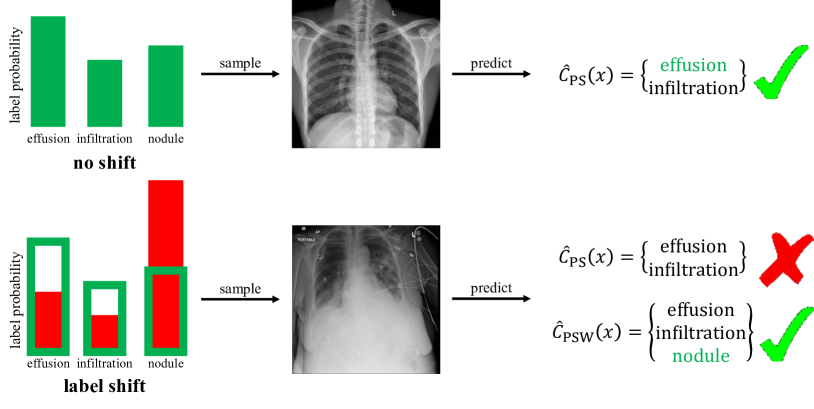
Figure 1: An example of our approach on the ChestX-ray dataset. In the unshifted setting, standard PAC prediction sets guarantee high-probability coverage, but this guarantee fails under label shift. Our approach addresses this challenge and remains valid in the shifted environment.

We empirically evaluate our approach on five datasets across three application domains: CIFAR-10 (Krizhevsky et al., 2009) and Entity-13 (Santurkar et al., 2020) in the computer vision domain, the CDC Heart Dataset (Centers for Disease Control and Prevention (1984), CDC) and ChestX-ray (National Institutes of Health and others, 2022) in the medical domain, and AGNews (Zhang et al., 2015) in the language domain.

Contributions. We propose a novel algorithm for constructing PAC prediction sets in the presence of label shift, which computes provably valid intervals around the true importance weights. Our algorithm is based on a novel technique for propagating confidence intervals through the updates of Gaussian elimination, which to the best of our knowledge is a novel approach to uncertainty propagation in a prediction set construction setting. This idea may be of independent interest and applicable to other linear algebraic computations. Finally, empirically demonstrate that our approach satisfies the PAC guarantee while constructing smaller prediction sets than several baselines.

Example. Figure 1 illustrates an application of our technique to the ChestX-ray dataset. In medical settings, PAC prediction sets (denoted PS) provide a rigorous way to quantify uncertainty for making downstream decisions; in particular, they guarantee that the prediction set contains the true label (in this case, a diagnosis) with high probability. However, label shift happens commonly in medical settings, for instance, many illnesses have varying rates of incidence over time even when the patient population remains the same. Unfortunately, label shift can invalidate the PAC coverage guarantee. Our approach (denoted PSW) corrects for the label shift via importance weighting; it does so in a provably correct way by propagating uncertainty through the Gaussian elimination computation used to construct importance weights. The resulting prediction sets satisfy the PAC guarantee.

Related work. There has been recent interest in conformal inference under distribution shift, much of it focusing on covariate shift (Tibshirani et al., 2019; Lei & Candès, 2021; Qiu et al., 2022). (Podkopaev & Ramdas, 2021) develop methods for marginal coverage under label shift, whereas we are interested in training-set conditional—or PAC—guarantees. Furthermore, they assume that the true importance weights are known, which is rarely the case. In the label shift setting, the importance weights can be estimated (Lipton et al., 2018), but as we show in our experiments, uncertainty in these estimates must be handled for the PAC guarantee to hold.

We leverage the method of (Park et al., 2021) to handle estimation error in the importance weights. That work studies covariate shift, and uses a heuristic to obtain intervals around the importance weights. For the label shift setting, we can in fact obtain stronger guarantees: we modify Gaussian elimination to propagate uncertainty through the computation of the weights $w^{*}=\mathbf{C}_{P}^{-1}q^{*}$. We give a more comprehensive discussion of related work in Appendix A. Our code is available at https://github.com/averysi224/pac-ps-label-shift for reproduction of our experiments.

2 Problem Formulation

2.1 Background on Label Shift

Consider the goal of training a classifier $g:\mathcal{X}\to\mathcal{Y}$, where $\mathcal{X}\subseteq\mathbb{R}^{d}$ is the covariate space, and $\mathcal{Y}=[K]=\{1,...,K\}$ is the set of labels. We consider the setting where we train on one distribution $P$ over $\mathcal{X}\times\mathcal{Y}$—called the source—with a probability density function (PDF) $p:(x,y)\mapsto p(x,y)$, and evaluate on a potentially different test distribution $Q$—called the target—with PDF $q:(x,y)\mapsto q(x,y)$. We focus on the unsupervised domain adaptation setting (Ben-David et al., 2007), where we are given an i.i.d. sample $S_{m}\sim P^{m}$ of $m$ labeled datapoints, and an i.i.d. sample of $n$ unlabeled datapoints $T_{X}^{n}\sim Q_{X}^{n}$. The label shift setting (Lipton et al., 2018) assumes that only the label distribution $Q_{Y}$ may change from $P_{Y}$, and the conditional covariate distributions remain the same:

Assumption 2.1.

(Label shift) We have $p(x\mid y)=q(x\mid y)$ for all $x\in\mathcal{X},y\in\mathcal{Y}$.

We denote $p(y)=P_{Y}(Y=y)$ for all $y\in\mathcal{Y}$ and analogously for $Q$. (Lipton et al., 2018) consider two additional mild assumptions:

Assumption 2.2.

For all $y\in\mathcal{Y}$ such that $q(y)>0$, we have $p(y)>0$.

Next, given the trained classifier $g:\mathcal{X}\rightarrow\mathcal{Y}$ let $\mathbf{C}_{P}\in\mathbb{R}^{K\times K}$ denote its expected confusion matrix—i.e., $c_{ij}:=(\mathbf{C}_{P})_{ij}=\mathbb{P}_{(X,Y)\sim P}(g(X)=i,Y=j)$.

Assumption 2.3.

The confusion matrix $\mathbf{C}_{P}$ is invertible.

This last assumption requires that the per-class expected predictor outputs be linearly independent; for instance, it is satisfied when $g$ is reasonably accurate across all labels. In addition, one may test whether this assumption holds (Lipton et al., 2018).

Denoting the importance weights $w^{*}\coloneqq(q(y)/p(y))_{y\in\mathcal{Y}}\in\mathbb{R}^{K}$, and $\hat{y}:=g(x)$, we will write $p(\hat{y}|y)=\mathbb{P}_{(X,Y)\sim P_{X}}[g(X)=\hat{y}|Y=y]$, and define $p(\hat{y},y)$, $p_{\hat{y}}$ as well as the corresponding expressions for $q$ analogously. Since $\hat{y}$ depends only on $x$, we have $q(\hat{y}\mid y)=p(\hat{y}\mid y)$. Thus, see e.g., Lipton et al. (2018),

$$q_{\hat{y}}=\sum_{y\in\mathcal{Y}}q(\hat{y}\mid y)q(y)=\sum_{y\in\mathcal{Y}}p(\hat{y}\mid y)q(y)=\sum_{y\in\mathcal{Y}}p(\hat{y},y)\frac{q(y)}{p(y)},$$

or in a matrix form, $q^{*}=\mathbf{C}_{P}w^{*}$, where $q^{*}\coloneqq(q_{\hat{y}})_{\hat{y}\in\mathcal{Y}}\in\mathbb{R}^{K}$. As we assume $\mathbf{C}_{P}$ is invertible,

$$w^{*}=\mathbf{C}_{P}^{-1}q^{*}.$$ (1)

Our algorithm uses this equation to approximate $w^{*}$, and then use its approximation to construct PAC prediction sets that remain valid under label shift.

2.2 PAC Prediction Sets Under Label Shift

We are interested in constructing a prediction set $C:\mathcal{X}\to 2^{\mathcal{Y}}$, which outputs a set of labels $C(x)\subseteq\mathcal{Y}$ for each given input $x\in\mathcal{X}$ rather than a single label. The benefit of outputting a set of labels is that we can obtain correctness guarantees such as:

$$\mathbb{P}_{(X,Y)\sim P}[Y\in C(X)]\geq 1-\varepsilon,$$ (2)

where $\varepsilon\in(0,1)$ is a user-provided confidence level. Then, downstream decisions can be made in a way that accounts for all labels $y\in C(x)$ rather than for a single label. Thus, prediction sets quantify uncertainty. Intuitively, equation 2 can be achieved if we output $C(x)=\mathcal{Y}$ for all $x\in\mathcal{X}$, but this is not informative. Instead, the typical goal is to output prediction sets that are as small as possible.

The typical strategy for constructing prediction sets is to leverage a fixed existing model. In particular, we assume given a scoring function $f:\mathcal{X}\times\mathcal{Y}\to\mathbb{R}$; most deep learning algorithms provide such scores in the form of predicted probabilities, with the corresponding classifier being $g(x)=\operatorname*{\arg\max}_{y\in\mathcal{Y}}f(x,y)$. The scores do not need to be reliable in any way; if they are unreliable, the PAC prediction set algorithm will output larger sets. Then, we consider prediction sets parameterized by a real-valued threshold $\tau\in\mathbb{R}$:

$$C_{\tau}(x)=\{y\in\mathcal{Y}\mid f(x,y)\geq\tau\}.$$

In other words, we include all labels with score at least $\tau$. First, we focus on correctness for $P$, in which case we only need $S_{m}$, usually referred to as the calibration set. Then, a prediction set algorithm constructs a threshold $\hat{\tau}(S_{m})\in\mathbb{R}$ and returns $C_{\hat{\tau}(S_{m})}$.

Finally, we want $\hat{\tau}$ to satisfy (2); one caveat is that it may fail to do so due to randomness in $S_{m}$. Thus, we allow an additional probability $\delta\in\mathbb{R}$ of failure, resulting in the following desired guarantee:

$$\mathbb{P}_{S_{m}\sim P^{m}}[\mathbb{P}_{(X,Y)\sim P}[Y\in C_{\hat{\tau}(S_{m})}(X)]\geq 1-\varepsilon]\geq 1-\delta.$$ (3)

Vovk (2012); Park et al. (2019) propose an algorithm $\hat{\tau}$ that satisfies (3), see Appendix B.

Finally, we are interested in constructing PAC prediction sets in the label shift setting, using both the labeled calibration dataset $S_{m}\sim P^{m}$ from the source domain, and the unlabeled calibration dataset $T_{n}^{X}\sim Q^{n}$ from the target distribution. Our goal is to construct $\hat{\tau}(S_{m},T_{n}^{X})$ based on both $S_{m}$ and $T_{n}^{X}$, which satisfies the coverage guarantee over $Q$ instead of $P$:

$$\mathbb{P}_{S_{m}\sim P^{m},T^{X}_{n}\sim Q^{n}_{X}}\left[\mathbb{P}_{(X,Y)\sim Q}[Y\in C_{\hat{\tau}(S_{m},T_{n}^{X})}(X)]\geq 1-\varepsilon\right]\geq 1-\delta.$$ (4)

Importantly, the inner probability is over the shifted distribution $Q$ instead of $P$.

3 Algorithm

To construct prediction sets valid under label shift, we first notice that it is enough to find element-wise confidence intervals for the importance weights $w^{*}$. Suppose that we can construct $W=\prod_{k\in\mathcal{Y}}[\underline{w}_{k},\overline{w}_{k}]\subseteq\mathbb{R}^{K}$ such that $w^{*}\in W$. Then, when adapted to our setting, the results of Park et al. (2021)—originally for the covariate shift problem—provide an algorithm that returns a threshold $\hat{\tau}(S_{m},V,W,b)$, where $V\sim\text{Uniform}([0,1])^{K}$ is a vector of random variables, such that

$$\mathbb{P}_{S_{m}\sim P^{m},V\sim U^{K}}\left[\mathbb{P}_{(X,Y)\sim Q}[Y\in C_{\hat{\tau}(S_{m},V,W,b)}]\geq 1-\varepsilon\right]\geq 1-\delta.$$ (5)

This is similar to equation 4 but one minor point is that it accounts for the randomness used by our algorithm—via $V$—in the outer probability. We give details in Appendix C.

The key challenge is to construct the elementwise confidence interval $W=\prod_{k\in\mathcal{Y}}[\underline{w}_{k},\overline{w}_{k}]$ such that $w^{*}\in W$ with high probability. The approach from Park et al. (2021) for the covariate shift problem relies on training a source-target discriminator, which is not possible in our case since we do not have class labels from the target domain. Furthermore, Park et al. (2021) do not provide conditions under which one can provide a valid confidence interval for the importance weights.

Our algorithm uses a novel approach, where we propagate intervals through the computation of importance weights. The weights $w^{*}$ are determined by the system of linear equations $\mathbf{C}_{P}w^{*}=q^{*}$. Since $\mathbf{C}_{P}$ and $q^{*}$ are unknown, we start by constructing element-wise confidence intervals

$$\underline{\mathbf{C}}_{P}\leq\mathbf{C}_{P}\leq\overline{\mathbf{C}}_{P}\qquad\text{and}\qquad\underline{q}^{*}\leq q^{*}\leq\overline{q}^{*},$$ (6)

with a probability of at least $1-\delta$ over our calibration datasets $S_{m}$ and $T_{n}^{X}$. We then propagate these confidence intervals through each step of Gaussian elimination, such that at the end of the algorithm, we obtain confidence intervals for its output—i.e.,

$$\underline{w}^{*}\leq w^{*}\leq\overline{w}^{*}\qquad\text{with probability at least}~{}1-\delta.$$ (7)

Finally, we can use (7) with the algorithm from (Park et al., 2021) to construct PAC prediction sets under label shift. We describe our approach below.

3.1 Elementwise Confidence Intervals for $\mathbf{C}_{P}$ and $q^{*}$

Recall that $\mathbf{C}_{P}=(c_{ij})_{ij\in\mathcal{Y}}$ and $q^{*}=(q_{\hat{y}})_{{\hat{y}}\in\mathcal{Y}}$. Note that $c_{ij}=\mathbb{P}[g(X)=i,Y=j]$ is the mean of the Bernoulli random variable $\mathbbm{1}(g(X)=i,Y=j)$ over the randomness in $(X,Y)\sim P$. Similarly, $q_{k}$ is the mean of $\mathbbm{1}(g(X)=k)$ over the randomness in $X\sim Q_{X}$. Thus, we can use the Clopper-Pearson (CP) intervals (Clopper & Pearson, 1934) for a Binomial success parameter to construct intervals around $c_{ij}$ and $q_{k}$. Given a confidence level $\delta\in(0,1)$ and the sample mean $\hat{c}_{ij}=\frac{1}{m}\sum_{(x,y)\in S_{m}}\mathbbm{1}(g(x)=i,y=j)$—distributed as a scaled Binomial random variable—this is an interval $\text{CP}(\hat{c}_{ij},m,\delta)=[\underline{c}_{ij},\overline{c}_{ij}]$ such that

$$\mathbb{P}_{S_{m}\sim P^{m}}[c_{ij}\in\text{CP}(\hat{c}_{ij},m,\delta)]\geq 1-\delta.$$

Similarly, for $q_{k}$, we can construct CP intervals based on $\hat{q}_{k}=\frac{1}{n}\sum_{x\in T_{n}^{X}}\mathbbm{1}(g(x)=k)$. Together, for confidence levels $\delta_{ij}$ and $\delta_{k}$ chosen later, we obtain for all $i,j,k\in[K]$,

$$\mathbb{P}_{S_{m}\sim P^{m}}\left[\underline{c}_{ij}\leq c_{ij}\leq\overline{c}_{ij}\right] \geq 1-\delta_{ij},\qquad\mathbb{P}_{T_{n}^{X}\sim Q_{X}^{n}}\left[\underline{q}_{k}\leq q_{k}\leq\overline{q}_{k}\right]\geq 1-\delta_{k}.$$

Then, the following result holds by a union bound: Given any $\delta_{ij},\delta_{k}\in(0,\infty)$, for all $i,j,k\in[K]$, letting $[\underline{c}_{ij},\overline{c}_{ij}]=\text{CP}(\hat{c}_{ij},m,\delta_{ij})$ and $[\underline{q}_{k},\overline{q}_{k}]=\text{CP}(\hat{q}_{k},n,\delta_{k})$, and letting $\delta=\sum_{i,j\in[K]}\delta_{ij}+\sum_{k\in[K]}\delta_{k}$, we have

$$\mathbb{P}_{S_{m}\sim P^{m},T_{n}^{X}\sim Q_{X}^{n}}\left[\bigwedge_{i,j\in[K]}\underline{c}_{ij}\leq c_{ij}\leq\overline{c}_{ij},\bigwedge_{k\in[K]}\underline{q}_{k}\leq q_{k}\leq\overline{q}_{k}\right]\geq 1-\delta.$$ (8)

3.2 Gaussian Elimination with Intervals

We also need to set up notation for Gaussian elimination, which requires us to briefly recall the algorithm. To solve $\mathbf{C}_{P}w^{*}=q^{*}$, Gaussian elimination (see e.g., Golub & Van Loan, 2013) proceeds in two phases. Starting with $c^{0}=\mathbf{C}_{P}$ and $q^{0}=q^{*}$, on iteration $t\geq 1$, Gaussian elimination uses row $k=t$ to eliminate the $k$th column of rows $i\in\{k+1,...,K\}$ (we introduce a separate variable $k$ for clarity). In particular, if $c_{kk}^{t}\neq 0$, we denote

$$c_{ij}^{t+1} =\begin{cases}c_{ij}^{t}-\dfrac{c_{ik}^{t}c_{kj}^{t}}{c_{kk}^{t}}&\text{if }i>k,\\ c_{ij}^{t}&\text{otherwise;}\end{cases}\qquad\,q_{i}^{t+1}=\begin{cases}q_{i}^{t}-\dfrac{c_{ik}^{t}q_{k}^{t}}{c_{kk}^{t}}&\text{if }i>k\\ q_{i}^{t}&\text{otherwise,}\end{cases}\qquad\forall i,j\in[K].$$

If $c_{kk}^{t}=0$, but there is an element $j>k$ in the $k$th column such that $c_{jk}^{t}\neq 0$, the $k$th and the $j$th rows are swapped and the above steps are executed. If no such element exists, the algorithm proceeds to the next step. At the end of the first phase, the matrix $c^{K-1}$ has all elements below the diagonal equal to zero—i.e., $c^{K-1}_{ij}=0$ if $j<i$. In the second phase, the Gaussian elimination algorithm solves for $w_{i}^{*}$ backwards from $i=K$ to $i=1$, introducing the following notation. For each $i$, if $c_{ii}^{K-1}\neq 0$, we denote $w_{i}^{*}=(q_{i}-s_{i})/c_{ii}^{K-1}$, where $s_{i}=\sum_{j=i+1}^{K}c_{ij}^{K-1}w_{j}^{*}$.

In our setting, we do not know $c^{0}$ and $q^{0}$; instead, we assume given entrywise confidence intervals as in equation 6, which amount to $\underline{c}^{0}\leq c^{0}\leq\overline{c}^{0}$ and $\underline{q}^{0}\leq q^{0}\leq\overline{q}^{0}$. We now work on the event $\Omega$ that these bounds hold, and prove that our algorithm works on this event; later, we combine this result with Equation 8 to obtain a high-probability guarantee. Then, our goal is to compute $\underline{c}^{t},\overline{c}^{t},\underline{q}^{t},\overline{q}^{t}$ such that for all iterations $t\in\{0,1,...,K-1\}$, we have elementwise confidence intervals specified by $\underline{c}^{t},\overline{c}^{t}$, $\underline{q}^{t}$ and $\overline{c}^{t}$ for the outputs $c^{t},q^{t}$ of the Gaussian elimination algorithm:

$$\underline{c}^{t}\leq c^{t}\leq\overline{c}^{t}\qquad\text{and}\qquad\underline{q}^{t}\leq q^{t}\leq\overline{q}^{t}.$$ (9)

The base case $t=0$ holds by the assumption. Next, to propagate the uncertainty through the Gaussian elimination updates for each iteration $t\in[K-1]$, our algorithm sets

$$\underline{c}_{ij}^{t+1} =\begin{cases}0&\text{if }i>k,~{}j\leq k,\\ \underline{c}_{ij}^{t}-\dfrac{\overline{c}_{ik}^{t}\overline{c}_{kj}^{t}}{\underline{c}_{kk}^{t}}&\text{if }i,j>k,\\ \underline{c}_{ij}^{t}&\text{otherwise}\end{cases}\qquad\forall i,j\in[K]$$ (10)

for the lower bound, and computes

$$\overline{c}_{ij}^{t+1} =\begin{cases}0&\text{if }i>k,~{}j\leq k,\\ \overline{c}_{ij}^{t}-\dfrac{\underline{c}_{ik}^{t}\underline{c}_{kj}^{t}}{\overline{c}_{kk}^{t}}&\text{if }i,j>k,\\ \overline{c}_{ij}^{t}&\text{otherwise}\end{cases}\qquad\forall i,j\in[K]$$ (11)

for the upper bound. The first case handles the fact that Gaussian elimination is guaranteed to zero out entries below the diagonal, and thus these entries have no uncertainty remaining. The second rule constructs confidence intervals based on the previous intervals and the algebraic update formulas used in Gaussian elimination for the entries for which $i,j>k$. For instance, the above confidence intervals use that on the event $\Omega$, and by induction on $t$, if $\underline{c}_{ij}^{t}\geq 0$ and $\underline{c}_{ii}^{t}>0$ for all $i,j\in[K]$ and for all $t$, the Gaussian elimination update $c_{ij}^{t+1}=c_{ij}^{t}-c_{it}^{t}c_{tj}^{t}/c_{tt}^{t}$ can be upper bounded as

$$c_{ij}^{t+1}=c_{ij}^{t}-\dfrac{c_{it}^{t}c_{tj}^{t}}{c_{tt}^{t}}\leq\overline{c}_{ij}^{t}-\dfrac{\underline{c}_{it}^{t}\underline{c}_{tj}^{t}}{\overline{c}_{tt}^{t}}=\overline{c}_{ij}^{t+1},$$ (12)

The assumptions that $\underline{c}_{ij}^{t}\geq 0$ and $\underline{c}_{ii}^{t}>0$ for all $i,j\in[K]$ and for all $t$ may appear a little stringent, but the former can be removed at the cost of slightly larger intervals propagated to the next step, see Section D. The latter condition is satisfied by any classifier that obtains sufficient accuracy on all labels. We further discuss these conditions in Section D. The third rule in equation 10 and equation 11 handles the remaining entries, which do not change; and thus the confidence intervals from the previous step can be used. The rules for $q$ are similar, and have a similar justification:

$$\underline{q}_{i}^{t+1}=\begin{cases}\underline{q}_{i}^{t}-\dfrac{\overline{c}_{ik}^{t}\overline{q}_{i}^{t}}{\underline{c}_{kk}^{t}}&\text{if }i>k,\\ \underline{q}_{i}^{t}&\text{otherwise;}\end{cases}\qquad\overline{q}_{i}^{t+1}=\begin{cases}\overline{q}_{i}^{t}-\dfrac{\underline{c}_{ik}^{t}\underline{q}_{i}^{t}}{\overline{c}_{kk}^{t}}&\text{if }i>k,\\ \overline{q}_{i}^{t}&\text{otherwise.}\end{cases}\qquad\forall i\in[K].$$ (13)

For these rules, our algorithm assumes $\underline{q}_{i}^{t}\geq 0$ for all $i\in[K]$ and all $t$, and raises an error if this fails. As with the first condition above, this one can be straightforwardly relaxed; see Appendix D.

In the second phase, we compute $w_{i}^{*}$ starting from $i=K$ and iterating to $i=1$. On iteration $i$, we assume we have the confidence intervals $\underline{w}_{j}^{*}\leq w_{j}^{*}\leq\overline{w}_{j}^{*}$ for $j>i$. Then, we compute confidence intervals for the sum $s_{i}$, which again have a similar justification based on the Gaussian elimination updates:

$$\underline{s}_{i}=\sum_{j=i+1}^{n}\underline{c}_{ij}^{K-1}\underline{w}_{j}^{*}\qquad\text{and}\qquad\overline{s}_{i}=\sum_{j=i+1}^{n}\overline{c}_{ij}^{K-1}\overline{w}_{j}^{*},$$ (14)

and show that they satisfy $\underline{s}_{i}\leq s_{i}\leq\overline{s}_{i}$ on the event $\Omega$. Finally, we compute confidence intervals for $w_{i}^{*}$, assuming $\underline{c}_{ii}^{K-1}>0$:

$$\underline{w}_{i}^{*}=\frac{\underline{q}_{i}-\overline{s}_{i}}{\overline{c}_{ii}^{K-1}}\qquad\text{and}\qquad\overline{w}_{i}^{*}=\frac{\overline{q}_{i}-\underline{s}_{i}}{\underline{c}_{ii}^{K-1}},$$ (15)

for which we can show that they satisfy $\underline{w}_{i}^{*}\leq w_{i}^{*}\leq\overline{w}_{i}^{*}$ based on the Gaussian elimination updates. Letting $W=\{w\mid\underline{w}^{*}\leq w\leq\overline{w}^{*}\}$, we have the following (see Appendix E for a proof).

Lemma 3.1 (Elementwise Confidence Interval for Importance Weights).

If (6) holds, and for all $i,j,t\in[K]$, $\underline{c}_{ij}^{t}\geq 0$, $\underline{c}_{ii}^{t}>0$, and $\underline{q}_{i}^{t}\geq 0$, then $w^{*}=\mathbf{C}_{P}^{-1}q^{*}\in W$.

We mention here that the idea of algorithmic uncertainty propagation may be of independent interest. In future work, it may further be developed to other methods for solving linear systems (e.g., the LU decomposition, Golub & Van Loan (2013)), and other linear algebraic and numerical computations.

3.3 Overall Algorithm

Algorithm 1 PS-W: PAC prediction sets in the label shift setting.

1:procedure LabelShiftPredictionSet($S_{m},T^{X}_{n},f,\varepsilon,\delta$)

2:     $\underline{c},\overline{c},\underline{q},\overline{q}\leftarrow$ CPInterval($S_{m},T^{X}_{n},x\mapsto\operatorname*{\arg\max}_{y\in\mathcal{Y}}f(x,y),\frac{K(K+1)}{(K(K+1)+1)}\delta$)

3:     $W\leftarrow$ IntervalGaussianElim($\underline{c},\overline{c},\underline{q},\overline{q}$)

4:     if $W=\varnothing$ then return $\varnothing$      

5:     return IWPredictionSet($S_{m},f,W,\varepsilon,\delta/[K(K+1)+1]$)

6:procedure CPInterval($S_{m},T^{X}_{n},g,\delta$)

7:     for $i,j\in[K]$ do

8:         Compute $[\underline{c}_{ij},\overline{c}_{ij}]=\text{CP}\left(m^{-1}\sum_{(x,y)\in S_{m}}\mathbbm{1}(g(x)=i,y=j),m,\delta/(K(K+1))\right)$      

9:     for $k\in[K]$ do

10:         Compute $[\underline{q}_{k},\overline{q}_{k}]=\text{CP}\left(n^{-1}\sum_{x\in T_{n}^{X}}\mathbbm{1}(g(x)=k),n,\delta/(K(K+1))\right)$      

11:     return $\underline{c},\overline{c},\underline{q},\overline{q}$

12:procedure IntervalGaussianElim($\underline{c}^{0},\overline{c}^{0},\underline{q}^{0},\overline{q}^{0}$)

13:     for $t\in[1,...,K-1]$ do

14:         for $i,j\in[K]$ do

15:              Compute $\underline{c}_{ij}^{t},\overline{c}_{ij}^{t}$ using (10) & (11), and $\underline{q}_{i}^{t},\overline{q}_{i}^{t}$ using (13)

16:              if $\underline{c}_{ij}^{t}<0$ for some $i\neq j$ or $\underline{c}_{ii}^{t}\leq 0$ for some $i$ or $\underline{q}_{i}^{t}\leq 0$ for some $i$, then return $\varnothing$                        

17:         for $i\in[K,...,1]$ do

18:              Compute $\underline{s}_{i}^{t},\overline{s}_{i}^{t}$ using (14), and $\underline{w}_{i},\overline{w}_{i}$ using (15)               

19:     return $W=\prod_{i=1}^{k}[\underline{w}_{i},\overline{w}_{i}]$

20:procedure IWPredictionSet($S_{m},f,W=\prod_{k=1}^{K}[\underline{w}_{k},\overline{w}_{k}],\varepsilon,\delta$)

21:     $V\sim\text{Uniform}([0,1])^{m}$

22:     return $\hat{\tau}(S_{m},V,W,\max_{k\in[K]}\overline{w}_{k},\varepsilon,\delta)$ as in (17)

Algorithm 1 summarizes our approach. As can be seen, the coverage levels for the individual Clopper-Pearson intervals are chosen to satisfy the overall $1-\delta$ coverage guarantee. In particular, the PAC guarantee equation 4 follows from equation 5, equation 8, Lemma 3.1, and a union bound.

Theorem 3.2 (PAC Prediction Sets under Label Shift).

For any given $\varepsilon,\delta\in(0,1)$, under Assumptions 2.1, 2.2 and 2.3, if $\forall i,j,t\in[K]$, we have $\underline{c}_{ij}^{t}\geq 0$, $\underline{c}_{ii}^{t}>0$, and $\underline{q}_{i}^{t}\geq 0$, then Algorithm 1 satisfies

$$\mathbb{P}_{S_{m}\sim P^{m},T_{n}^{X}\sim Q^{n},V\sim U^{m}}\left[\mathbb{P}_{(X,Y)\sim Q}[Y\in C_{\hat{\tau}(S_{m},V,W,b)}(X)]\geq 1-\varepsilon\right]\geq 1-\delta.$$

As discussed in Appendix D, we can remove the requirement that $\underline{c}_{ij}^{t}\geq 0$ and $\underline{q}_{i}^{t}\geq 0$ for $i\neq j$.

4 Experiments

4.1 Experimental Setup

Predictive models. We analyze five datasets: the CDC Heart dataset, CIFAR-10, Chest X-ray, AG News, and the Entity-13 dataset; their details are provided in Section 4.2. We use a two-layer MLP for the CDC Heart data with an SGD optimizer having a learning rate of $0.03$ and a momentum of $0.9$, a batch size of $64$ for $30$ epochs. For CIFAR-10, we finetuned a pretrained ResNet50 He et al. (2016), with a learning rate of $0.01$ for $56$ epochs. For the ChestX-ray14 dataset, we use a pre-trained CheXNet (Rajpurkar et al., 2017) with a DenseNet121 (Huang et al., 2017) backbone with learning rate $0.0003$ for $2$ epochs. For AGNews, a pre-trained Electra sequence classifier fine-tuned for one epoch with an AdamW optimizer using a learning rate of $0.00001$ is used. For the Entity-13 dataset, we finetuned a pretrained ResNet50, with a learning rate of $0.01$ for $13$ epochs.

Hyperparameter choices. There are two user-specified parameters that control the guarantees, namely $\delta$ and $\varepsilon$. In our experiments, we choose $\delta=5\times 10^{-4}$ to ensure that, over 100 independent datasets $S_{m}$, there is a 95% probability that the error rate is not exceeded. Specifically, this ensures that $\mathbb{P}_{(X,Y)\sim P}[Y\in C_{\hat{\tau}(S_{m})}(X)]\geq 1-\varepsilon$ holds for all 100 trials, with probability approximately $1-0.95^{1/100}\approx 5\times 10^{-4}$. We select multiple $\varepsilon$s for each dataset in a grid search way, demonstrating the validity of our algorithm.

Dataset construction. We follow the label shift simulation strategies from previous work (Lipton et al., 2018). First, we split the original dataset into training, source base, and target base. We use the training dataset to train the score function. Given label distributions $P_{Y}$ and $Q_{Y}$, we generate the source dataset $S_{m}$, target dataset $T_{n}^{X}$, and a labeled size $o$ target test dataset (sampled from $Q$) by sampling with replacement from the corresponding base dataset. We consider two choices of $P_{Y}$ and $Q_{Y}$: (i) a tweak-one shift, where we assign a probability to one of the labels, and keep the remaining labels equally likely, and (ii) arbitrary shift, where we shift each probability as described later.

Baselines. We compare our approach (PS-W) with several baselines (see Appendix G):

• PS: PAC prediction sets that do not account for label shift (Vovk, 2012; Park et al., 2019). This does not come with PAC guarantees under label shift.

• WCP: Weighted conformal prediction under label shift, which targets marginal coverage (Podkopaev & Ramdas, 2021). This does not come with PAC guarantees under label shift either.

• PS-R: PAC prediction sets that account for label shift but ignore uncertainty in the importance weights; which does not come with PAC guarantees under label shift come with.

• PS-C: Addresses label shift via a conservative upper bound on the empirical loss (see Appendix G for details). This is the only baseline to come with PAC guarantees under label shift.

We compare to other baselines in Appendix H.6, and to an oracle with the true weights in Appendix F, more results for different hyperparameters are in Appendix H.

Metrics. We measure performance via the prediction set error, i.e., the fraction of $(x,y)\sim Q$ such that $y\notin C_{\tau}(x)$; and the average prediction set size, i.e., the mean of $|C_{\tau}(x)|$, evaluated on the held-out test set. We report the results over $100$ independent repetitions, randomizing both dataset generation and our algorithm.

4.2 Results & Discussion

CDC heart. We use the CDC Heart dataset, a binary classification problem (Centers for Disease Control and Prevention (1984), CDC), to predict the risk of heart attack given features such as level of exercise or weight. We consider both large and small shifts.

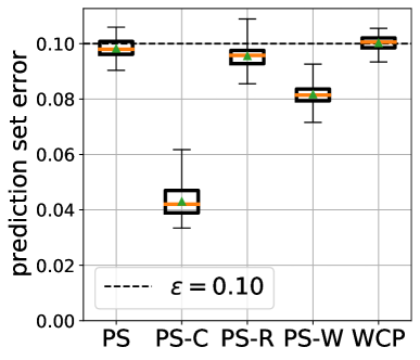
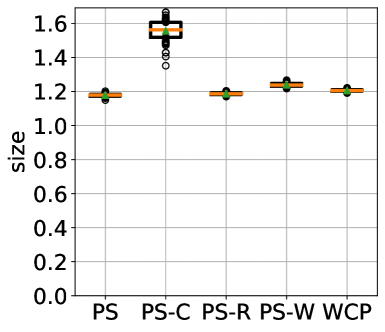
(a) Prediction set error and size under small shifts on the CDC Heart dataset . Parameters are $\varepsilon=0.1$, $\delta=5\times 10^{-4}$ , $m=42000$, $n=42000$, and $o=9750$.

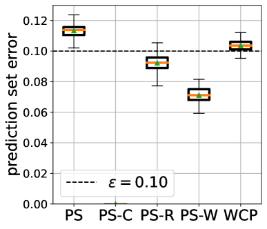
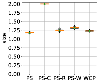
(b) Prediction set error and size under large shifts on the CDC Heart dataset. Parameters are $\varepsilon=0.1$, $\delta=5\times 10^{-4}$, $m=42000$, $n=42000$, and $o=9750$.

Figure 2: Prediction set results on the CDC Heart dataset

For the large shift, the label distributions (denoted $(\text{pos}\%,\text{neg}\%)$) are $(94\%,6\%)$ for source, and $(63.6\%,36.4\%)$ for target; results are in Figure 2(b). We also consider a small shift with label distributions $(94\%,6\%)$ for source, and $(91.3\%,8.7\%)$ for target; results for $\varepsilon=0.1$ are in Figure 2(a). As can be seen, our PS-W algorithm satisfies the PAC guarantee while achieving smaller prediction set size than PS-C, the only baseline to satisfy the PAC guarantee. The PS and PS-R algorithms violate the PAC guarantee .

CIFAR-10. Next, we consider CIFAR-10 (Krizhevsky et al., 2009), which has 10 labels. We consider a large and a small tweak-one shift. For the large shift, the label probability is 10% for all labels in the source, 40.0% for the tweaked label, and 6.7% for other labels in the target; results are in Figure 3(a). For small shifts, we use 10% for all labels for the source, 18.2% for the tweaked label, and 9.1% for other labels for the target; results for $\varepsilon=0.1$ are in Figure 3(b). Under large shifts, our PS-W algorithm satisfies the PAC guarantee while outperforming PS-C by a large margin. When the shift is very small, PS-W still satisfies the PAC guarantee, but generates more conservative prediction sets similar in size to those of PS-C (e.g., Figure 3(b)) given the limited data.

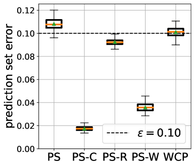
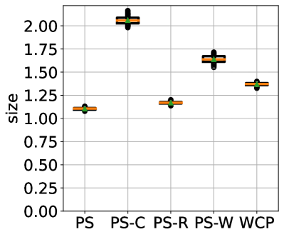
(a) Prediction set error and size with larger shift on CIFAR-10. Parameters are $\varepsilon=0.1$, $\delta=5\times 10^{-4}$, $m=27000$, $n=19997$, and $o=19997$.

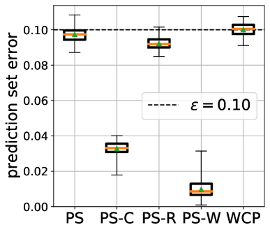
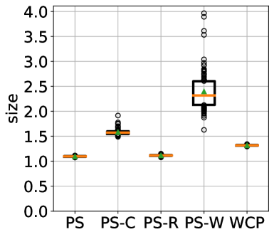
(b) Prediction set error and size with small shift on CIFAR-10. Parameters are $\varepsilon=0.1$, $\delta=5\times 10^{-4}$, $m=27000$, $n=16500$, and $o=16500$.

Figure 3: Prediction set results on CIFAR-10.

AGNews. AG News is a subset of AG’s corpus of news articles (Zhang et al., 2015). It is a text classification dataset with four labels: World, Sports, Business, and Sci/Tech. It contains 31,900 unique examples for each class. We use $\varepsilon=0.05$ and tweak-one label shifts. We consider a large shift and a medium-sized calibration dataset, with label distributions equalling $(30.8\%,30.8\%,7.7\%,30.8\%)$ for the source, and $(12.5\%,12.5\%,62.5\%,12.5\%)$ for the target; results are in Figure 4(a). As before, our PS-W approach satisfies the PAC guarantee while achieving smaller set sizes than PS-C.

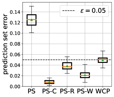
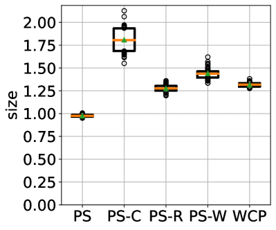
(a) Prediction set error and size on the AGNews Dataset. Parameters are $\varepsilon=0.05$, $\delta=5\times 10^{-4}$, $m=26000$, $n=12800$, and $o=12800$.

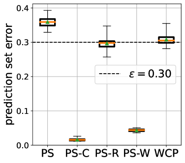
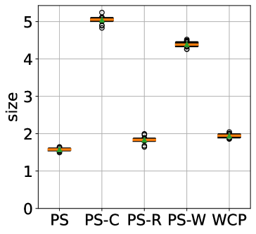
(b) Prediction set error and size on the ChestX-ray dataset. Parameters are $\varepsilon=0.3$, $\delta=5\times 10^{-4}$, $m=67200$, $n=35200$, and $o=3520$.

Entity-13 Entity-13 is a part of the BREEDs benchmark (Santurkar et al., 2020), which leverages the class hierarchy in ImageNet (Deng et al., 2009) to repurpose the original classes into superclasses Entity-13 contains 13 superclasses and a total of 390k images. It is also included in a recent label shift benchmark for relaxed label shift, RLSBench (Garg et al., 2023). We consider a general label shift and, additionally, a small shift with a medium-sized calibration dataset. The label probabilities equal $7.7\%$ each in the source and $(7.1\%,[3.6\%]*4,10.71\%,3.6\%,7.1\%,43.69\%,[3.6\%]*4)$ in the target. Results for $\varepsilon=0.1$ is shown in Figure 5. As before, our PS-W approach satisfies the PAC guarantee while outperforming PS-C. The PS-R and WCP methods violate the constraint.

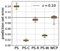
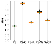
Figure 5: Prediction set error and size on the Entity-13 dataset. Parameters are $\varepsilon=0.1$, $\delta=5\times 10^{-4}$, $m=52000$, $n=21000$, and $o=4667$.

ChestX-ray. ChestX-ray14 (Wang et al., 2017) is a medical imaging dataset containing about 112K frontal-view X-ray images of 30K unique patients with fourteen disease labels. This dataset contains instances with multiple labels, which we omit. We also omit classes with few positively labeled datapoints, leaving $6$ classes: Atelectasis, Effusion, Infiltration, Mass, Nodule, Pneumothorax. We consider a large tweak-one shift, with label distributions of $([19.1\%]*4,4.5\%,19.1\%)$ for the source, and $([11.1\%]*4,44.5\%,11.1\%)$ for the target. Results for $\varepsilon=0.3$ are in Figure 4(b). As before, our PS-W approach satisfies the PAC guarantee while outperforming PS-C.

Discussion. In all our experiments, our approach satisfies the PAC guarantee; furthermore, it produces smaller prediction set sizes than PS-C—the only baseline to consistently satisfy the PAC guarantee—except when the label shift is small and the calibration dataset is limited. In contrast, the PS baseline does not account for label shift, and the PS-R baseline does not account for uncertainty in the importance weights, so they do not satisfy the PAC guarantee. The WCP baseline is designed to target a weaker guarantee, so it naturally does not satisfy the PAC guarantee. Thus, these results demonstrate the efficacy of our approach.

5 Conclusion

We have proposed a PAC prediction set algorithm for the label shift setting that accounts for confidence intervals around importance weights by modifying Gaussian elimination to propagate intervals. Our algorithm provides provable PAC guarantees and produces smaller prediction sets than several baselines that satisfy this condition. Experiments on five datasets demonstrate its effectiveness. Directions for future work include improving performance when the calibration dataset is small or when the label shift is small.

Appendix A Additional Related Work

Conformal Prediction. Our work falls into the broad area of distribution-free uncertainty quantification  (Guttman, 1970). Specifically, it builds on ideas from conformal prediction (Vovk et al., 2005; Balasubramanian et al., 2014; Angelopoulos & Bates, 2021), which aims to construct prediction sets with finite sample guarantees. The prediction sets are realized by a setting a threshold on top of a traditional single-label predictor (i.e. conformity/non-conformity scoring function) and predicting all labels with scores above the threshold. Our approach is based on inductive conformal prediction (Papadopoulos et al., 2002; Vovk, 2012; Lei et al., 2015), where the dataset is split into a training set for training the scoring function and a calibration set for constructing the prediction sets.

PAC Prediction Sets. Unlike conformal prediction methods that achieve a coverage guarantee of the median coverage performance. PAC prediction sets consider training-data conditional correctness (Vovk, 2012; Park et al., 2019). That is, we achieve a $(\varepsilon,\delta)$-guarantee that our performance on all future possible examples would only exceed the desired error rate level $\varepsilon$ with probability under $\delta$. This guarantee is also equivalent to the “content” guarantee for tolerance regions (Wilks, 1941; Fraser, 1956). All in all, PAC prediction sets obtain a totally different statistical guarantee compared to conformal prediction methods. The preference of the two methods depends on the application scenario. Obviously, PAC prediction sets favor the case when even a slight excess of the desired error rate would cause a significant safety concern.

	Covariate Shift	Label Shift
Importance weights	$q(x)/p(x)$	$q(y)/p(y)$
Invariance	$p(y\mid x)=q(y\mid x)$	$p(x\mid y)=q(x\mid y)$

Table 1: Comparison of covariate shift and label shift.

Label shift. Label shift (Zadrozny, 2004; Huang et al., 2006; Sugiyama et al., 2007; Gretton et al., 2009) is a kind of distribution shift; in contrast to the more widely studied covariate shift, it assumes the conditional covariate distribution is fixed but the label distribution may change; see Table 1. In more detail, letting $p$ and $q$ denote the probability density function of the source and target domains, respectively, we assume that $q(y)$ may be shifted compared to $p(y)$, but $p(x\mid y)=q(x\mid y)$. Label shift can arise when sets of classes change (e.g., their frequency increases) in scenarios like medical diagnosis and object recognition (Storkey et al., 2009; Saerens et al., 2002; Lipton et al., 2018).

Early solutions required estimation of $q(x),p(x\mid y)$, often relying on kernel methods, which may scale poorly with data size and dimension (Chan & Ng, 2005; Storkey et al., 2009; Zhang et al., 2013). More recently, two approaches achieved scalability by assuming an approximate relationship between the classifier outputs $\hat{y}$ and ground truth labels $y$ (Lipton et al., 2018; Azizzadenesheli et al., 2019; Saerens et al., 2002): Black Box Shift Estimation (BBSE) (Lipton et al., 2018) and RLLS (Azizzadenesheli et al., 2019) provided consistency results and finite-sample guarantees assuming the confusion matrix is invertible. Subsequent work developed a unified framework that decomposes the error in computing importance weights into miscalibration error and estimation error, with BBSE as a special case (Garg et al., 2020); this approach was extended to open set label shift domain adaptation (Garg et al., 2022).

Conformal methods and distribution shift. Due to its distribution-free nature, conformal prediction has been successfully dealing with distribution shift problem. Previous works mainly focus on covariate shift (Tibshirani et al., 2019; Lei & Candès, 2021; Qiu et al., 2022). (Podkopaev & Ramdas, 2021) considers label shift; however, they assume that the true importance weights are exactly known, which is rarely the case in practice. While importance weights can be estimated, there is typically uncertainty in these estimates that must be accounted for, especially in high dimensions.

The rigorous guarantee of PAC prediction sets requires quantifying the uncertainty in each part of the system. Thus, we apply a novel linear algebra method to obtain the importance weights confidence intervals for the uncertainty of label shift estimation. This setting has been studied in the setting of covariate shift (Park et al., 2021), but under a much simpler distribution structure. In contrast, the data structure of label shift problem is more complex in the unsupervised label shift setting.

More broadly, prediction sets have been studied in the meta-learning setting (Dunn et al., 2022; Park et al., 2022), as well as the setting of robustness to all distribution shifts with bounded $f$-divergence (Cauchois et al., 2020).

Class-conditional prediction sets. Although not designed specifically for solving the label shift problem, methods for class-conditional coverage (Sadinle et al., 2019) and adaptive prediction sets (APS) (Romano et al., 2020) can improve robustness to label shifts. However, class-conditional coverage is a stronger guarantee that leads to prediction sets larger than for our algorithm, while APS does not satisfy a PAC guarantee; we compare to these approaches in Appendix H.6.

Appendix B Background on PAC Prediction Sets

Finding the maximum $\tau$ that satisfies (3) is equivalent to choosing $\tau$ such that the empirical error

$$\bar{L}_{S_{m}}(C_{\tau}):=\sum_{(x,y)\in S_{m}}\mathbbm{1}(y\notin C_{\tau}(x))$$

on the calibration set $S_{m}$ is bounded (Vovk et al., 2005; Park et al., 2019). Let $F(k;m,\varepsilon)=\sum^{k}_{i=0}\binom{m}{k}\varepsilon^{i}(1-\varepsilon)^{m-i}$ be the cumulative distribution function (CDF) of the binomial distribution $\text{Binom}(m,\varepsilon)$ with $m$ trials and success probability $\varepsilon$ evaluated at $k$. Then, Park et al. (2019) constructs $C_{\hat{\tau}}$ via

$$\hat{\tau}=\max_{\tau\in T}\tau\quad\text{subj. to}\quad\bar{L}_{S_{m}}(C_{\tau})\leq k(m,\varepsilon,\delta),$$ (16)

$$\text{where}~{}~{}k(m,\varepsilon,\delta)=\max_{k\in\mathbb{N}\cup\{0\}}k~{}~{}\text{subj. to}~{}~{}F(k;m,\varepsilon)\leq\delta.$$

Their approach is equivalent to the method from Vovk (2012), but formulated in the language of learning theory. By viewing the prediction set as a binary classifier, the PAC guarantee via this construction can be connected to the Binomial distribution. Indeed, for fixed $C$, $\bar{L}_{S_{m}}(C)$ has distribution $\text{Bionm}(m,L_{P}(C))$, since $\mathbbm{1}(y\notin C(x))$ has a $\text{Bernoulli}(L_{P}(C))$ distribution when $(x,y)\sim P$. Thus, $k(m,\varepsilon,\delta)$ defines a bound such that if $L_{P}(C)\leq\varepsilon$, then $\bar{L}_{S_{m}}(C)\leq k(m,\varepsilon,\delta)$ with probability at least $1-\delta$.

Appendix C Background on Prediction Sets Under Distribution Shift

Here we demonstrate how to obtain prediction sets given intervals $\underline{w}^{*}\leq w^{*}\leq\overline{w}^{*}$ around the true importance weights. This approach is based closely on the strategy in (Park et al., 2021) for constructing prediction sets under covariate shift, but adapts it to the label shift setting (indeed, our setting is simpler since there are finitely many importance weights). The key challenge is computing the importance weight intervals, which we describe in detail below.

Given the true importance weights $w^{*}$, one strategy would be to use rejection sampling (Von Neumann, 1951; Shapiro, 2003; Rubinstein & Kroese, 2016) to subsample $S_{m}$ to obtain a dataset that effectively consists of $N\leq m$ i.i.d. samples from $Q$ (here, $N$ is a random variable, but this turns out not to be an issue). Essentially, for each $(x_{i},y_{i})\in S_{m}$, we sample a random variable $V_{i}\sim\text{Uniform}([0,1])$, and then accept samples where $V_{i}\geq w_{y_{i}}^{*}/b$, where $b$ is an upper bound on $w_{y}^{*}$:

$$T_{N}(S_{m},V,w^{*},b)=\left\{(x_{i},y_{i})\in S_{m}\biggm{|}V_{i}\geq\frac{w_{y_{i}}^{*}}{b}\right\}.$$

In our setting, we can take $b=\max_{y\in\mathcal{Y}}w_{y}^{*}$. Then, we return $\hat{\tau}(T_{N}(S_{m},V,w^{*},b))$. Since $T_{N}(S_{m},V,w^{*},b)$ consists of an i.i.d. sample from $Q$, we obtain the desired PAC guarantee (4).

In practice, we do not know the true importance weights $w^{*}$. Instead, suppose we can obtain intervals $W_{y}=[\underline{w}_{y}^{*},\overline{w}_{y}^{*}]$ such that $w_{y}^{*}\in W_{y}$ with high probability. We let $W=\prod_{y\in\mathcal{Y}}W_{y}$, and assume $w^{*}\in W$ with probability at least $1-\delta$. The algorithm proposed in (Park et al., 2021) adjusts the above algorithm to conservatively account for this uncertainty—i.e., it chooses $\tau$ so the PAC guarantee (4) holds for any importance weights $w\in W$:

$$\hat{\tau}(S_{m},V,W,b)=\min_{w\in W}\hat{\tau}(T_{N}(S_{m},V,w,b)).$$ (17)

We minimize over $\tau$ since choosing smaller $\tau$ leads to larger prediction sets, which is more conservative. (Park et al., 2021) show how to compute (17) efficiently. We have the following guarantee:

Theorem C.1 (Theorem 4 in (Park et al., 2021)).

Assume that $w^{*}\in W$. Letting $U=\text{Uniform}([0,1])$,

$$\mathbb{P}_{S_{m}\sim P^{m},V\sim U^{m}}\left[\mathbb{P}_{(X,Y)\sim Q}[y\in C_{\hat{\tau}(S_{m},V,W,b)}]\geq 1-\varepsilon\right]\geq 1-\delta.$$

In other words, the PAC guarantee (4) holds, with the modification that the outer probability includes the randomness over the samples $V\sim U^{m}$ used by our algorithm.

Appendix D Ensuring the Confidence Bounds at each Step

The diagonal elements $c_{kk}$ of the confusion matrix of an accurate classifier, are typically much larger than the other elements. Indeed, for an accurate classifier, the probabilities of correct predictions $c_{kk}=P(g(x)=k,y=k)$ are higher than those of incorrect predictions $c_{ik}:=P(g(x)=i,y=k),i\neq k$. On the other hand, the Clopper-Pearson interval is expected to be short (for instance, the related Wald interval has length or order $1/\sqrt{m}$, where $m$ is the sample size). Thus, we expect that

$$\overline{c}^{0}_{ik}\ll\underline{c}^{0}_{kk},k=1,\dots,K,i\neq k.$$ (18)

Without loss of generality, we consider equation 10 as an example. In the Gaussian elimination process, recall that the update at step $t$ is

$$\underline{c}_{ij}^{t+1}=\underline{c}_{ij}^{t}-\dfrac{\overline{c}^{t}_{ik}}{\underline{c}_{kk}^{t}}\overline{c}_{kj}^{t}\quad\text{if }i,j>k.$$ (19)

Combining with equation 18, the factor by which the $k$-th row is multiplied is small, i.e., $\overline{c}^{t}_{ik}/\underline{c}^{t}_{kk}\ll 1$. Thus the resulting $i$-th diagonal elements

$$\underline{c}_{ii}^{t+1}=\underline{c}_{ii}^{t}-\dfrac{\overline{c}^{t}_{ik}}{\underline{c}_{kk}^{t}}\overline{c}_{ki}^{t}$$

change little after each elimination step, and are expected to remain positive. Next we discuss intervals for off-diagonal elements.

Balanced classifier. For a balanced classifier, when $c_{ik}$ and $c_{jk}$ are close for all $i,j$ such that $i\neq k$, $j\neq k$, since the factor $\overline{c}^{t}_{ik}/\underline{c}^{t}_{kk}$ is small, the lower bound in equation 19 is expected to be positive.

Imbalanced classifier. For the more general case of a possibly imbalanced classifier, $c_{ij}$ and $c_{kj}$ may not be close. This could cause non-positive bounds at certain steps, so the confidence interval may not be valid at the next steps; e.g., equation 12 may fail. However, note that since

$$c_{ik}^{t}\in[\underline{c}_{ik}^{t},\overline{c}_{ik}^{t}],\quad c_{kj}^{t}\in[\underline{c}_{kj}^{t},\overline{c}_{kj}^{t}],$$

we have

$$c_{ik}^{t}c_{kj}^{t}\leq\max\{|\underline{c}_{ik}^{t}|,|\overline{c}_{ik}^{t}|\}\cdot\max\{|\underline{c}_{kj}^{t}|,|\overline{c}_{kj}^{t}|\}$$

and hence

$$\frac{c_{ik}^{t}c_{kj}^{t}}{c_{kk}^{t}}\leq\frac{\max\{|\underline{c}_{ik}^{t}|,|\overline{c}_{ik}^{t}|\}\cdot\max\{|\underline{c}_{kj}^{t}|,|\overline{c}_{kj}^{t}|\}}{\underline{c}_{kk}^{t}}.$$

In fact, one can derive the even tighter bound

$$\max\left(\dfrac{\overline{c}_{ik}^{t}\overline{c}_{kj}^{t}}{\underline{c}_{kk}^{t}},\dfrac{\underline{c}_{ik}^{t}\overline{c}_{kj}^{t}}{\underline{c}_{kk}^{t}},\dfrac{\underline{c}_{ik}^{t}\underline{c}_{kj}^{t}}{\underline{c}_{kk}^{t}},\dfrac{\overline{c}_{ik}^{t}\underline{c}_{kj}^{t}}{\underline{c}_{kk}^{t}},\dfrac{\overline{c}_{ik}^{t}\overline{c}_{kj}^{t}}{\overline{c}_{kk}^{t}},\dfrac{\underline{c}_{ik}^{t}\overline{c}_{kj}^{t}}{\overline{c}_{kk}^{t}},\dfrac{\underline{c}_{ik}^{t}\underline{c}_{kj}^{t}}{\overline{c}_{kk}^{t}},\dfrac{\overline{c}_{ik}^{t}\underline{c}_{kj}^{t}}{\overline{c}_{kk}^{t}}\right).$$

This can be checked by carefully going through all possible cases of positive and negative values of the bounds. Similar changes can be made to computing the upper bounds.

It is possible for our final interval $W$ to contain negative lower bounds due to loose element-wise intervals or other factors. Since importance weights are non-negative, negative importance weight bounds act the same way as zero lower bounds in rejection sampling, and preserve our guarantees.

Finally, the requirement of an accurate classifier is already imposed by methods such as BBSE to ensure the invertibility of the confusion matrix. Therefore, our Gaussian elimination approach does not impose significantly stronger assumptions.

Appendix E Proof of Lemma 3.1

For the first phase, we prove by induction on $t$ that (9) holds for all $t$. The base case $t=0$ holds by assumption. For the induction step, we focus on $\underline{c}_{ij}^{t+1}$; the remaining bounds $\overline{c}_{ij}^{t+1}$, $\underline{q}_{k}^{t+1}$, and $\overline{q}_{k}^{t+1}$ follow similarly. There are three sub-cases i, each corresponding to one of the update rules in (10). For the first update rule $\overline{c}_{ij}^{t+1}=0$, equation 9 follows since the Gaussian elimination algorithm guarantees that $c_{ij}^{t+1}=0$. For the second and third update rules, equation 9 follows by direct algebra and the induction hypothesis. For instance, for $i,j>t$, equation 12 holds, and similarly $c_{ij}^{t+1}\geq\underline{c}_{ij}^{t+1}$.

For the second phase, the fact that $\underline{s}\leq s\leq\overline{s}$ and $\underline{w}^{*}\leq w^{*}\leq\overline{w}^{*}$ follows by a similar induction argument. Since Gaussian elimination guarantees that $w^{*}=\mathbf{C}_{P}^{-1}q^{*}$, and we have shown that $w^{*}\in W=\prod_{i=1}^{K}[\underline{w}_{i},\overline{w}_{i}]$, the claim follows. ∎

Appendix F Oracle Importance Weight Results

Here, we show comparisons to an oracle that is given the ground truth importance weights (which are unknown and must be estimated in most practical applications). It uses rejection sampling according to these weights rather than conservatively accounting for uncertainty in the weights.

First, for the CDC heart dataset, we consider the following label distributions: source $(94\%,6\%)$, target: $(63.6\%,36.4\%)$; see Figure 6(a) for the results. Second, for the CIFAR-10 dataset, we consider the following label distributions: source $(10\%,10\%,10\%,10\%,10\%$, $10\%,10\%$, $10\%,10\%,10\%)$, target: $(6.7\%,6.7\%,6.7\%,40.0\%,6.7\%,6.7\%,6.7\%,6.7\%,6.7\%,6.7\%)$; see Figure 6(b) for results.

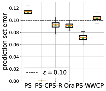
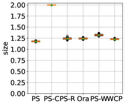
(a) Prediction set error and size on the CDC dataset. Parameters are $\varepsilon=0.1$, $\delta=5\times 10^{-4}$, $m=42000$, $n=42000$, and $o=9750$.

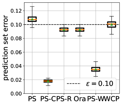
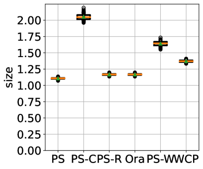
(b) Prediction set error and size on CIFAR10. Parameters are $\varepsilon=0.1$, $\delta=5\times 10^{-4}$, $m=27000$, $n=19997$, and $o=19997$.

Figure 6: Prediction set results with comparison to the oracle importance weight (Ora).

Appendix G Conservative Baseline

We describe PS-C, the conservative baseline summarized in Algorithm 2. In particular, given an upper bound $b\geq w^{*}$ on the importance weight, we use the upper bound

$$\mathbb{E}_{(X,Y)\sim P}[\ell(g(X),Y)\cdot w_{Y}^{*}]\leq b\cdot\mathbb{E}_{(X,Y)\sim P}[\ell(g(X),Y)].$$

As a consequence, we can run the original prediction set algorithm from Vovk (2012); Park et al. (2019) with a more conservative choice of $\varepsilon$ that accounts for this upper bound.

Algorithm 2 PS-C: an algorithm using the CP bound in equation 20.

1:procedure PS-C($S_{m},T^{X}_{n},f,\mathcal{T},\varepsilon,\delta_{w},\delta_{C}$)

2:     $\underline{c},\overline{c},\underline{q},\overline{q}\leftarrow$ CPInterval($S_{m},T^{X}_{n},x\mapsto\operatorname*{\arg\max}_{y\in\mathcal{Y}}f(x,y),\delta_{w}$)

3:     $W\leftarrow$ IntervalGaussianElim($\underline{c},\overline{c},\underline{q},\overline{q}$)

4:     $b\leftarrow\max_{k\in[K]}\overline{w}_{k}$

5:     return PS($S_{m},f,\mathcal{T},\varepsilon/b,\delta_{C}$)

Lemma G.1.

Algorithm 2 satisfies the PAC guarantee under label shift equation 4.

Proof.

Having constructed the importance weight intervals $w^{*}$, we can use $b=\max_{k\in[K]}\overline{w}_{k}$ to find a conservative upper bound on the risk as follows:

$$E_{(X,Y)\sim Q}[\mathbbm{1}(Y\notin C_{\tau}(X)]=\int q(x,y)\mathbbm{1}(y\notin C_{\tau}(x))dxdy$$

$$=\int p(x,y)w(y)\mathbbm{1}(y\notin C_{\tau}(x))dxdy\leq bE_{(X,Y)\sim P}[\mathbbm{1}(Y\notin C_{\tau}(X)].$$ (20)

Hence, using the PS prediction set algorithm with parameters $(\varepsilon/b,\delta)$, the output is $(\varepsilon,\delta)$-PAC. ∎

Appendix H More Results

H.1 CDC Heart

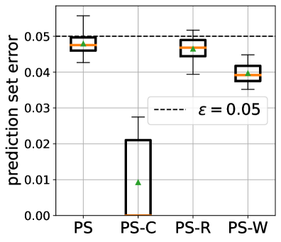
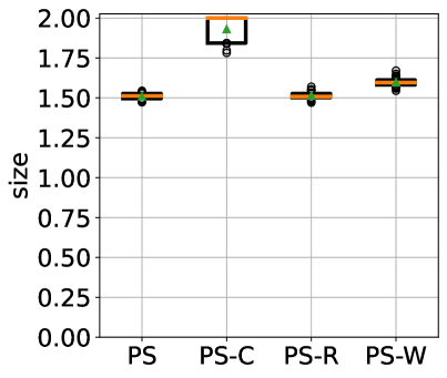
(a) Prediction set error and size under small shifts on the CDC Heart dataset. Parameters are $\varepsilon=0.05$, $\delta=5\times 10^{-4}$ , $m=42000$, $n=42000$, and $o=9750$.

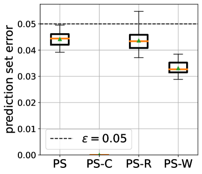
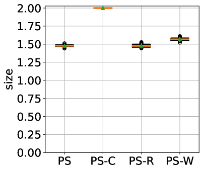
(b) Prediction set error and size under large shifts on the CDC Heart dataset, Parameters are $\varepsilon=0.05$, $\delta=5\times 10^{-4}$, $m=42000$, $n=42000$, and $o=9750$.

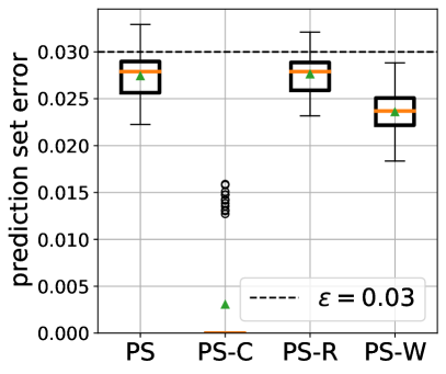
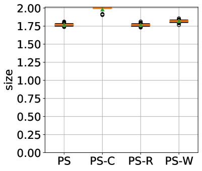
(c) Prediction set error and size under small shifts on the CDC Heart dataset. Parameters are $\varepsilon=0.03$, $\delta=5\times 10^{-4}$ , $m=42000$, $n=42000$, and $o=9750$.

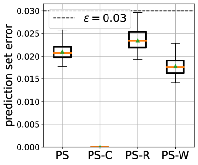
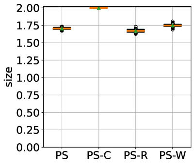
(d) Prediction set error and size under large shifts on the CDC Heart dataset, Parameters are $\varepsilon=0.03$, $\delta=5\times 10^{-4}$, $m=42000$, $n=42000$, and $o=9750$.

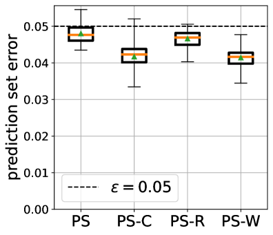
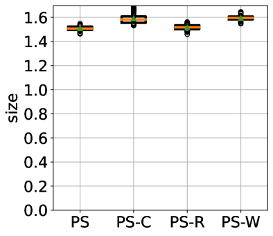
(e) Prediction set error and size under reversed small shifts $((91.3\%,8.7\%)\rightarrow(94\%,6\%))$ on the CDC Heart dataset. Parameters are $\varepsilon=0.05$, $\delta=5\times 10^{-4}$ , $m=42000$, $n=42000$, and $o=9750$.

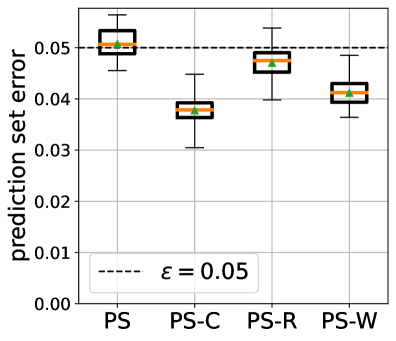
(f) Prediction set error and size under reversed large shifts $((63.6\%,36.4\%)\rightarrow(94\%,6\%))$ on the CDC Heart dataset, Parameters are $\varepsilon=0.03$, $\delta=5\times 10^{-4}$, $m=42000$, $n=42000$, and $o=9750$.

Figure 7: More Prediction set results with different hyperparameters on the CDC Heart dataset.

H.2 CIFAR-10

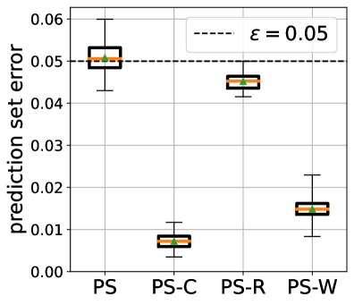
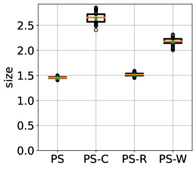
(a) Prediction set error and size with large shifts on CIFAR-10. Parameters are $\varepsilon=0.05$, $\delta=5\times 10^{-4}$, $m=27000$, $n=19997$, and $o=19997$.

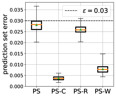
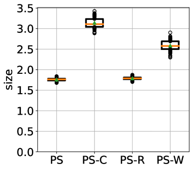
(b) Prediction set error and size with large shifts on CIFAR-10. Parameters are $\varepsilon=0.03$, $\delta=5\times 10^{-4}$, $m=27000$, $n=19997$, and $o=19997$.

Figure 8: More Prediction set results with different hyperparameters on the CIFAR-10 dataset.

H.3 AGNews

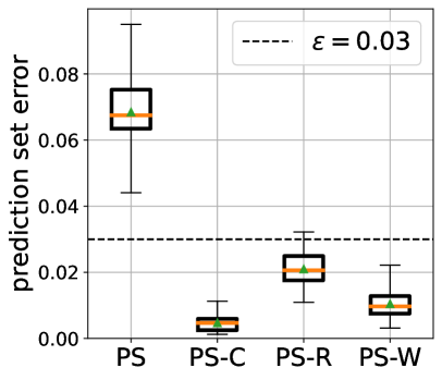
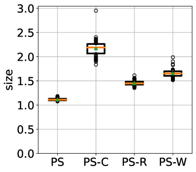
(a) Prediction set error and size on the AGNews Dataset. Parameters are $\varepsilon=0.03$, $\delta=5\times 10^{-4}$, $m=26000$, $n=12800$, and $o=12800$.

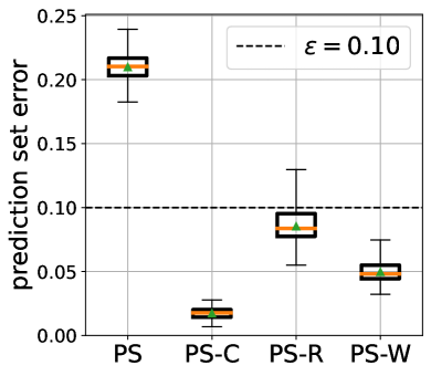
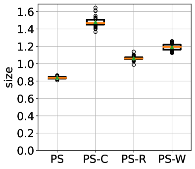
(b) Prediction set error and size on the AGNews Dataset. Parameters are $\varepsilon=0.1$, $\delta=5\times 10^{-4}$, $m=26000$, $n=12800$, and $o=12800$.

Figure 9: More Prediction set results with different hyperparameters on the AGNews dataset.

H.4 Entity-13

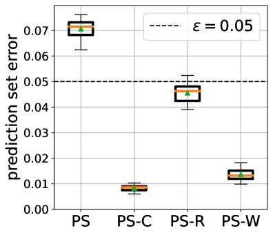
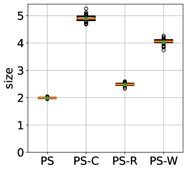
(a) Prediction set error and size on the Entity-13 dataset. Parameters are $\varepsilon=0.05$, $\delta=5\times 10^{-4}$, $m=52000$, $n=21000$, and $o=4667$.

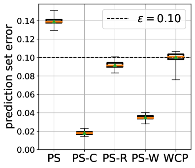
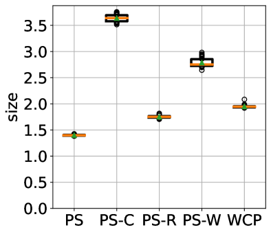
(b) Prediction set error and size on the Entity-13 dataset. Parameters are $\varepsilon=0.1$, $\delta=5\times 10^{-4}$, $m=52000$, $n=21000$, and $o=4667$.

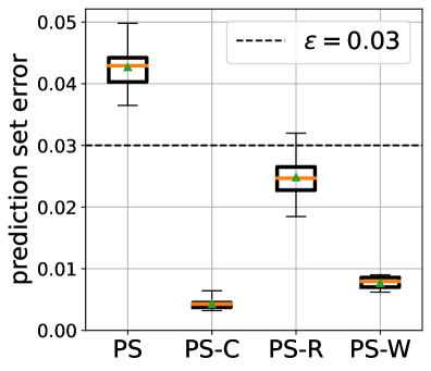
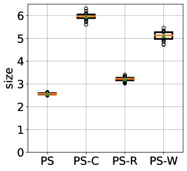
(c) Prediction set error and size on the Entity-13 dataset. Parameters are $\varepsilon=0.03$, $\delta=5\times 10^{-4}$, $m=52000$, $n=21000$, and $o=4667$.

Figure 10: More Prediction set results with different hyperparameters on the Entity-13 dataset.

H.5 ChestX-ray

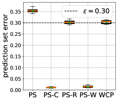
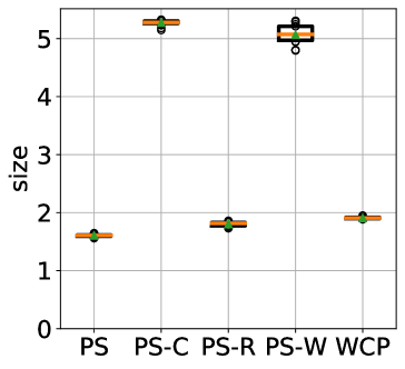
(a) Prediction set error and size on the ChestX-ray dataset. Parameters are $\varepsilon=0.3$, $\delta=5\times 10^{-4}$, $m=33600$, $n=17600$, and $o=3520$.

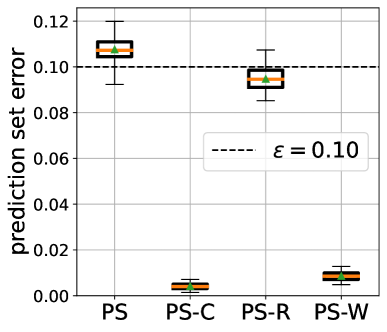
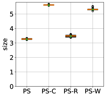
(b) Prediction set error and size on the ChestX-ray dataset. Parameters are $\varepsilon=0.1$, $\delta=5\times 10^{-4}$, $m=67200$, $n=35200$, and $o=3520$.

Figure 11: More Prediction set results with different hyperparameters on the ChestX-ray dataset.

H.6 Additional Baselines

Class-conditional conformal predictors fit separate thresholds for each label and demonstrate robustness to label shift. In Figure 12, we show the class-conditional results for both conformal prediction tuned for average coverage and our PAC prediction set, on the CDC dataset. Here, LWCP is a baseline from the label-conditional setting from Sadinle et al. (2019), which does not satisfy a PAC guarantee. PS-LW adapts the standard PAC prediction set algorithm Vovk (2012); Park et al. (2020) to the label-conditional setting; our approach is PS-W. Most relevantly, while PS-LW approximately satisfies the desired error guarantee, it is more conservative than our approach (PS-W) and produces prediction sets that are larger on average. Intuitively, it satisfies a stronger guarantee than necessary for our setting, leading it to be overly conservative.

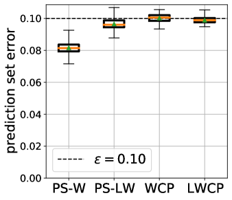
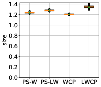
Figure 12: Prediction set error and size under small shifts on the CDC dataset. Parameters are $\varepsilon=0.1$, $\delta=5\times 10^{-4}$, $m=42000$, $n=42000$, and $o=9750$.

Empirically, we find that while APS improves coverage in the label shift setting, it does not satisfy our desired PAC guarantee. In particular, we show results for the APS scoring function with vanilla prediction sets in Figure 13; as can be seen, it does not satisfy the desired coverage guarantee. Due to its unusual structure, it is not clear how APS can be adapted to the PAC setting, which is our focus.

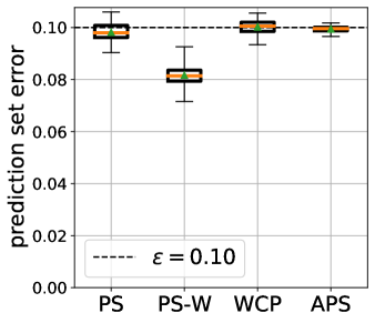
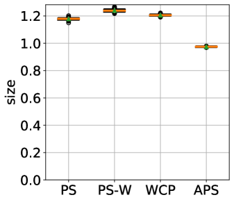
Figure 13: Prediction set error and size under small shifts on CDC dataset. Parameters are $\varepsilon=0.1$, $\delta=5\times 10^{-4}$, $m=42000$, $n=42000$, and $o=9750$.

References

- Angelopoulos & Bates (2021) Anastasios N Angelopoulos and Stephen Bates. A gentle introduction to conformal prediction and distribution-free uncertainty quantification. arXiv preprint arXiv:2107.07511, 2021.
- Azizzadenesheli et al. (2019) Kamyar Azizzadenesheli, Anqi Liu, Fanny Yang, and Animashree Anandkumar. Regularized learning for domain adaptation under label shifts. arXiv preprint arXiv:1903.09734, 2019.
- Balasubramanian et al. (2014) Vineeth Balasubramanian, Shen-Shyang Ho, and Vladimir Vovk. Conformal prediction for reliable machine learning: theory, adaptations and applications. Newnes, 2014.
- Ben-David et al. (2006) Shai Ben-David, John Blitzer, Koby Crammer, and Fernando Pereira. Analysis of representations for domain adaptation. Advances in neural information processing systems, 19, 2006.
- Ben-David et al. (2007) Shai Ben-David, John Blitzer, Koby Crammer, and Fernando Pereira. Analysis of representations for domain adaptation. In Advances in neural information processing systems, pp. 137–144, 2007.
- Cauchois et al. (2020) Maxime Cauchois, Suyash Gupta, Alnur Ali, and John C Duchi. Robust validation: Confident predictions even when distributions shift. arXiv preprint arXiv:2008.04267, 2020.
- Centers for Disease Control and Prevention (1984) (CDC) Centers for Disease Control and Prevention (CDC). Behavioral risk factor surveillance system, 1984. URL https://www.cdc.gov/brfss/annual_data/annual_data.htm.
- Chan & Ng (2005) Yee Seng Chan and Hwee Tou Ng. Word sense disambiguation with distribution estimation. In IJCAI, volume 5, pp. 1010–5, 2005.
- Clopper & Pearson (1934) Charles J Clopper and Egon S Pearson. The use of confidence or fiducial limits illustrated in the case of the binomial. Biometrika, 26(4):404–413, 1934.
- Deng et al. (2009) Jia Deng, Wei Dong, Richard Socher, Li-Jia Li, Kai Li, and Li Fei-Fei. Imagenet: A large-scale hierarchical image database. In 2009 IEEE conference on computer vision and pattern recognition, pp. 248–255. Ieee, 2009.
- Dunn et al. (2022) Robin Dunn, Larry Wasserman, and Aaditya Ramdas. Distribution-free prediction sets for two-layer hierarchical models. Journal of the American Statistical Association, 0(0):1–12, 2022.
- Fraser (1956) Donald Alexander Stuart Fraser. Nonparametric methods in statistics. John Wiley & Sons Inc, 1956.
- Garg et al. (2020) Saurabh Garg, Yifan Wu, Sivaraman Balakrishnan, and Zachary Lipton. A unified view of label shift estimation. Advances in Neural Information Processing Systems, 33:3290–3300, 2020.
- Garg et al. (2022) Saurabh Garg, Sivaraman Balakrishnan, and Zachary C Lipton. Domain adaptation under open set label shift. arXiv preprint arXiv:2207.13048, 2022.
- Garg et al. (2023) Saurabh Garg, Nick Erickson, James Sharpnack, Alex Smola, Sivaraman Balakrishnan, and Zachary Chase Lipton. Rlsbench: Domain adaptation under relaxed label shift. In International Conference on Machine Learning, pp. 10879–10928. PMLR, 2023.
- Golub & Van Loan (2013) Gene H Golub and Charles F Van Loan. Matrix computations. JHU press, 2013.
- Gretton et al. (2009) Arthur Gretton, Alex Smola, Jiayuan Huang, Marcel Schmittfull, Karsten Borgwardt, and Bernhard Schölkopf. Covariate shift by kernel mean matching. Dataset shift in machine learning, 3(4):5, 2009.
- Guttman (1970) I. Guttman. Statistical Tolerance Regions: Classical and Bayesian. Griffin’s statistical monographs & courses. Hafner Publishing Company, 1970. URL https://books.google.com/books?id=3Q7vAAAAMAAJ.
- He et al. (2016) Kaiming He, Xiangyu Zhang, Shaoqing Ren, and Jian Sun. Deep residual learning for image recognition. In Proceedings of the IEEE conference on computer vision and pattern recognition, pp. 770–778, 2016.
- Huang et al. (2017) Gao Huang, Zhuang Liu, Laurens Van Der Maaten, and Kilian Q Weinberger. Densely connected convolutional networks. In Proceedings of the IEEE conference on computer vision and pattern recognition, pp. 4700–4708, 2017.
- Huang et al. (2006) Jiayuan Huang, Arthur Gretton, Karsten Borgwardt, Bernhard Schölkopf, and Alex Smola. Correcting sample selection bias by unlabeled data. Advances in neural information processing systems, 19, 2006.
- Krizhevsky et al. (2009) Alex Krizhevsky, Geoffrey Hinton, et al. Learning multiple layers of features from tiny images. Technical report, University of Toronto, 2009.
- Lei et al. (2015) Jing Lei, Alessandro Rinaldo, and Larry Wasserman. A conformal prediction approach to explore functional data. Annals of Mathematics and Artificial Intelligence, 74(1):29–43, 2015.
- Lei & Candès (2021) Lihua Lei and Emmanuel J Candès. Conformal inference of counterfactuals and individual treatment effects. Journal of the Royal Statistical Society: Series B (Statistical Methodology), 2021.
- Lipton et al. (2018) Zachary Lipton, Yu-Xiang Wang, and Alexander Smola. Detecting and correcting for label shift with black box predictors. In International conference on machine learning, pp. 3122–3130. PMLR, 2018.
- National Institutes of Health and others (2022) National Institutes of Health and others. Nih clinical center provides one of the largest publicly available chest x-ray datasets to scientific community, 2022.
- Papadopoulos et al. (2002) Harris Papadopoulos, Kostas Proedrou, Volodya Vovk, and Alex Gammerman. Inductive confidence machines for regression. In European Conference on Machine Learning, pp. 345–356. Springer, 2002.
- Park et al. (2019) Sangdon Park, Osbert Bastani, Nikolai Matni, and Insup Lee. Pac confidence sets for deep neural networks via calibrated prediction. arXiv preprint arXiv:2001.00106, 2019.
- Park et al. (2020) Sangdon Park, Shuo Li, Insup Lee, and Osbert Bastani. Pac confidence predictions for deep neural network classifiers. arXiv preprint arXiv:2011.00716, 2020.
- Park et al. (2021) Sangdon Park, Edgar Dobriban, Insup Lee, and Osbert Bastani. Pac prediction sets under covariate shift. arXiv preprint arXiv:2106.09848, 2021.
- Park et al. (2022) Sangdon Park, Edgar Dobriban, Insup Lee, and Osbert Bastani. Pac prediction sets for meta-learning. arXiv preprint arXiv:2207.02440, 2022.
- Podkopaev & Ramdas (2021) Aleksandr Podkopaev and Aaditya Ramdas. Distribution-free uncertainty quantification for classification under label shift. In Uncertainty in Artificial Intelligence, pp. 844–853. PMLR, 2021.
- Qiu et al. (2022) Hongxiang Qiu, Edgar Dobriban, and Eric Tchetgen Tchetgen. Prediction sets adaptive to unknown covariate shift. arXiv preprint arXiv:2203.06126, 2022.
- Rajpurkar et al. (2017) Pranav Rajpurkar, Jeremy Irvin, Kaylie Zhu, Brandon Yang, Hershel Mehta, Tony Duan, Daisy Ding, Aarti Bagul, Curtis Langlotz, Katie Shpanskaya, et al. Chexnet: Radiologist-level pneumonia detection on chest x-rays with deep learning. arXiv preprint arXiv:1711.05225, 2017.
- Romano et al. (2020) Yaniv Romano, Matteo Sesia, and Emmanuel Candes. Classification with valid and adaptive coverage. Advances in Neural Information Processing Systems, 33:3581–3591, 2020.
- Rubinstein & Kroese (2016) Reuven Y Rubinstein and Dirk P Kroese. Simulation and the Monte Carlo method. John Wiley & Sons, 2016.
- Sadinle et al. (2019) Mauricio Sadinle, Jing Lei, and Larry Wasserman. Least ambiguous set-valued classifiers with bounded error levels. Journal of the American Statistical Association, 114(525):223–234, 2019.
- Saerens et al. (2002) Marco Saerens, Patrice Latinne, and Christine Decaestecker. Adjusting the outputs of a classifier to new a priori probabilities: a simple procedure. Neural computation, 14(1):21–41, 2002.
- Santurkar et al. (2020) Shibani Santurkar, Dimitris Tsipras, and Aleksander Madry. Breeds: Benchmarks for subpopulation shift. arXiv preprint arXiv:2008.04859, 2020.
- Shapiro (2003) Alexander Shapiro. Monte carlo sampling methods. Handbooks in operations research and management science, 10:353–425, 2003.
- Storkey et al. (2009) Amos Storkey et al. When training and test sets are different: characterizing learning transfer. Dataset shift in machine learning, 30:3–28, 2009.
- Sugiyama et al. (2007) Masashi Sugiyama, Shinichi Nakajima, Hisashi Kashima, Paul Buenau, and Motoaki Kawanabe. Direct importance estimation with model selection and its application to covariate shift adaptation. Advances in neural information processing systems, 20, 2007.
- Tibshirani et al. (2019) Ryan J Tibshirani, Rina Foygel Barber, Emmanuel Candes, and Aaditya Ramdas. Conformal prediction under covariate shift. Advances in neural information processing systems, 32, 2019.
- Von Neumann (1951) John Von Neumann. Various techniques used in connection with random digits. Appl. Math Ser, 12(36-38):3, 1951.
- Vovk (2012) Vladimir Vovk. Conditional validity of inductive conformal predictors. In Asian conference on machine learning, pp. 475–490. PMLR, 2012.
- Vovk et al. (2005) Vladimir Vovk, Alexander Gammerman, and Glenn Shafer. Algorithmic learning in a random world. Springer Science & Business Media, 2005.
- Wang et al. (2017) Xiaosong Wang, Yifan Peng, Le Lu, Zhiyong Lu, Mohammadhadi Bagheri, and Ronald M Summers. Chestx-ray8: Hospital-scale chest x-ray database and benchmarks on weakly-supervised classification and localization of common thorax diseases. In Proceedings of the IEEE conference on computer vision and pattern recognition, pp. 2097–2106, 2017.
- Wilks (1941) Samuel S Wilks. Determination of sample sizes for setting tolerance limits. The Annals of Mathematical Statistics, 12(1):91–96, 1941.
- Zadrozny (2004) Bianca Zadrozny. Learning and evaluating classifiers under sample selection bias. In Proceedings of the twenty-first international conference on Machine learning, pp. 114, 2004.
- Zhang et al. (2013) Kun Zhang, Bernhard Schölkopf, Krikamol Muandet, and Zhikun Wang. Domain adaptation under target and conditional shift. In International conference on machine learning, pp. 819–827. PMLR, 2013.
- Zhang et al. (2015) Xiang Zhang, Junbo Zhao, and Yann LeCun. Character-level convolutional networks for text classification. Advances in neural information processing systems, 28, 2015.