Multi-moiré trilayer graphene: lattice relaxation, electronic structure, and magic angles

Abstract

We systematically explore the structural and electronic properties of twisted trilayer graphene systems. In general, these systems are characterized by two twist angles, which lead to two incommensurate moiré periods. We show that lattice relaxation results in the formation of domains of periodic single-moiré structures only for twist angles close to the simplest fractions. For the majority of other twist angles, the incommensurate moiré periods lead to a quasicrystalline structure. We identify experimentally relevant magic angles at which the electronic density of states is sharply peaked and strongly correlated physics is most likely to be realized.

I Introduction

The electronic density of states (DOS) serves as a key predictor of strong electronic correlations for a wide range of many-body quantum systems. This principle is clearly illustrated by two foundational theories in condensed matter physics. First, the Stoner criterion, which posits that spontaneous ferromagnetism occurs when the DOS exceeds the inverse interaction energy scale. Second, the Bardeen–Cooper–Schrieffer (BCS) theory of superconductivity, where the transition temperature is a monotonically increasing function of the DOS. This principle has played out magnificently in twisted bilayer graphene where, following theoretical predictions of a “magic angle” at which the DOS exhibits a sharp peak [1, 2], experiments revealed a rich interacting phase diagram of correlated insulators, understood to be various forms of flavor ferromagnetism, along with regions of superconductivity[3, 4, 5, 6, 7, 8, 9, 10, 11, 12, 13, 14, 15, 16, 17, 18, 19, 20] These discoveries ushered a wave of experimental and theoretical activity in the field of moiré materials, now expanded beyond purely graphene, and has led to the experimental realization of a remarkably broad range of exotic strongly correlated states [21, 22].

While the majority of studies have focused on bilayer systems, going to three or more layers greatly increases the space of possibilities. The large parameter space of multilayer systems allows for systematic identification of which material properties are necessary for realizing various strongly correlated phenomena, such as superconductivity or orbital ferromagnetism. Gaining a better understanding of multilayer systems is therefore paramount to utilizing the full potential of twisted materials. However, the large and mostly unexplored phase space of multilayer systems also presents a practical barrier to efficient experimental exploration. Because of this, it is important to first determine the experimental parameters that are most likely to lead to correlated phenomena in multilayer devices.

We focus our attention on twisted trilayer graphene (TTG) systems, which are characterized by the two twist angles: the angle of rotation between the first and second layers ($\theta_{12}$), and between the second and third layers ($\theta_{23}$) [23, 24, 25, 26, 27, 28]. We will denote specific configurations with the ordered pair $(\theta_{12},\theta_{23})$. To avoid redundancy, we take $|\theta_{12}|<|\theta_{23}|$ throughout this work, as $\theta_{12}\rightarrow\theta_{23}$ when the graphene stack is inverted. As we will describe, this two-dimensional parameter space contains many distinct classes of systems, with present experiments showing a wide array of different physical phenomena.

The most well studied TTG systems are “single-moiré” structures, characterized by a single moiré periodicity shared among all layers. This is the case for the mirror symmetric $(\theta,-\theta)$ TTG [29, 30, 31]. Near the magic angle of $1.56^{\circ}$, the central bands become flat, and $\sim(1.6^{\circ},-1.6^{\circ})$-TTG has been found to exhibit strong correlations and superconductivity with reentrant behavior and possible Pauli limit violations  [32, 33, 34, 35, 36, 37, 38]. A single-moiré structure is also present in $(\theta,0)$-TTG (i.e. twisted monolayer-bilayer graphene), where topology and ferromagnetism have been observed at twist angles $\sim(1.1^{\circ},0)$[39, 40, 41, 42, 43, 20]. Additionally, if $\theta_{23}$ is significantly larger than $\theta_{12}$, the first layer effectively electronically decouples from other layers [44, 45], such that the only relevant moiré period is set by $\theta_{12}$. In Ref. 46, it was shown that $\sim(1.1^{\circ},-5.5^{\circ})$-TTG behaves like decoupled monolayer graphene and MATBG, and the flavor symmetry breaking commonly found in MATBG was observed.

Generally, TTG realizes a “multi-moiré” structure in which the moiré superlattices formed by $\theta_{12}$ and $\theta_{23}$ have different periods and/or orientations. Despite not having a single well-defined moiré periodicity, experimental studies have still found evidence of strong electronic interactions in multi-moiré systems, indicating that strict moiré periodicity is not a prerequisite for correlated physics. In Ref. 47, strong interactions in the form of a “Dirac revival”, indicative of flavor ferromagnetism, and regions of superconductivity were observed in $(1.4^{\circ},-1.9^{\circ})$-TTG, termed a “moiré quasicrystal”. Very recently, orbital ferromagnetism and an anomalous Hall effect were observed in “helical trilayer graphene”, $\sim(1.8^{\circ},1.8^{\circ})$-TTG [48]. Although the unrelaxed lattice structure of $(\theta,\theta)$-TTG exhibits a multi-moiré pattern, theoretical studies have shown that it relaxes into large domains (several hundreds of nanometers across) of a single-moiré structure separated by a triangular network of domain walls[49, 50, 51, 52]. The local band structure for these domains contains flat bands at a magic angle of $(1.85^{\circ},1.85^{\circ})$.

The TTG systems listed above are strikingly dissimilar in many ways: $(1.6^{\circ},-1.6^{\circ})$-TTG and $(1.1^{\circ},0)$-TTG are periodic, $(1.1^{\circ},-5.5^{\circ})$-TTG is effectively electronically periodic, $(1.8^{\circ},1.8^{\circ})$-TTG relaxes into periodic domains, and the $(1.4^{\circ},-1.9^{\circ})$-TTG is quasiperiodic. These systems also exhibit different physical phenomena. But in all cases, strongly correlated phases have been observed. A common thread between all these systems is a strongly peaked DOS appearing near a magic angle. We use this principle to comprehensively analyze an extensive class of multi-moiré TTG systems and identify experimentally relevant magic angles where strongly correlated phases are likely to be observed, guiding the way for future experimental exploration.

$\theta_{12}/\theta_{23}$	($\theta_{12}$, $\theta_{23}$)	Exp	$\theta_{12}/\theta_{23}$	($\theta_{12}$, $\theta_{23}$)	Exp
-1/1	$(1.56^{\circ},-1.56^{\circ})$	[30, 31, 32, 33, 34, 35, 36]	1/1	$(1.85^{\circ},1.85^{\circ})$	[48]
-3/4	$(1.41^{\circ},-1.88^{\circ})$	[47]	3/4	$(1.61^{\circ},2.14^{\circ})$	—
-2/3	$(1.32^{\circ},-1.99^{\circ})$	—	2/3	$(1.52^{\circ},2.28^{\circ})$	—
-1/2	$(1.22^{\circ},-2.44^{\circ})$	—	1/2	$(1.31^{\circ},2.61^{\circ})$	—
-1/3	$(1.16^{\circ},-3.48^{\circ})$	—	1/3	$(1.20^{\circ},3.61^{\circ})$	—
-1/4	$(1.13^{\circ},-4.52^{\circ})$	$\sim$ [46]	1/4	$(1.16^{\circ},\,4.64^{\circ})$	—

Table 1: First magic angles for TTG for simple angle ratios, and experiments where strongly correlated physics have been observed. The DOS is peaked within a range of $\sim\pm.05^{\circ}$ of the first magic angle.

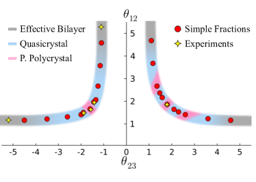
Figure 1: The TTG magic angles found in this work (red), where $\theta_{12}/\theta_{23}=\text{p}/\text{q}$ is a simple fraction. The simple fraction magic angles are connected by a “magic line”. For moderate values of $\theta_{12}$ and $\theta_{23}$ the system is either a periodic polycrystal (pink) or quasicrystal (blue). For large $\theta_{12}$ or $\theta_{23}$, (gray) one of the layers decouples, and the other two layers form an effective magic angle bilayer. Stars indicate twist angles where correlated phenomena have been observed in experiment: $(1.6^{\circ},-1.6^{\circ})$[32, 33, 34, 35, 36, 38], $(1.4^{\circ},-1.9^{\circ})$[47], $(1.1^{\circ},\sim-5.5^{\circ})$[46], and $(1.8^{\circ},1.8^{\circ})$[48]. Data is symmetrized with respect to exchange of the first and third layers.

We first explore the effect of lattice relaxation, which plays a crucial role in multi-moiré TTG systems due to the large supermoiré period. Our key result is that the relaxed structure of multi-moiré TTG systems, near the first magic angles, broadly fall into three categories, summarized in Fig. 1. (i) Supermoiré scale lattice relaxation results in the formation large domains of an energetically favorable single-moiré structure, separated by sharp domain walls. This structure resembles a polycrystal, but with a periodic arrangement of crystalline domains on the supermoiré scale. We thus refer to this as the “periodic polycrystalline” regime, which encompasses systems with twist angles close to $\theta_{12}/\theta_{23}\approx\pm 1$, and $\theta_{12}/\theta_{23}\approx 1/2$. (ii) Supermoiré lattice relaxation does not result in the formation of large single-moiré domains. We refer to this as the “quasicrystalline” regime, which encompasses much of the $(\theta_{12},\theta_{23})$ phase space away from the polycrystalline cases above (including MQC). (iii) Finally, when $|\theta_{12}|$ is significantly smaller than $|\theta_{23}|$, the third layer effectively decouples electronically, and the physics reduces to that of TBG. We refer to this as the effectively “bilayer” regime, which occurs for $|\theta_{12}/\theta_{23}|\lesssim 1/4$.

We further explore the electronic properties of multi-moiré TTG. When $\theta_{12}/\theta_{23}\approx\text{p}/\text{q}$ is close to a simple fraction, the local moiré-scale electronic properties can be well described by a generalized Bistritzer-MacDonald continuum model[29, 24, 53, 54, 55, 49], parameterized by a shift vector $\mathbf{d}$ between the two moiré superlattices. We explore the twist angle and $\mathbf{d}$ dependence of the DOS which, combined with the relaxed structure, allow us to identify magic angles at which the DOS is maximized, summarized in Table 1. We remark that, for systems that have already been explored experimentally, our magic angles agree quantitatively with the experimental angles at which strongly correlated states are found.

This paper is structured as follows: In Sec. II, we present lattice relaxation calculations for multi-moiré TTG and discuss how the relaxed lattice forms either a periodic polycrystal or a quasicrystal. In Sec. III, we analyze the electronic structure when the twist angles form a simple fraction, and determine magic angles where the DOS is peaked. We discuss the physical consequences and experimental relevance of our results in Sec. IV. We also provide several appendices that contain technical details of our results.

II Supermoiré Lattice Relaxation

Multi-moiré TTG systems are characterized by two twist angles, $\theta_{12}$ and $\theta_{23}$. Explicitly, if we label the twist of layer $l$ relative to some fixed orientation as $\theta_{l}$, then $\theta_{12}=\theta_{1}-\theta_{2}$ and $\theta_{23}=\theta_{2}-\theta_{3}$. This leads to two subclasses of multi-moiré TTG systems: those with alternating twist angles, $\theta_{12}/\theta_{23}<0$, and those with helical twist angles, $\theta_{12}/\theta_{23}>0$. In both cases, TTG is characterized by several length scales: the graphene lattice constant $a_{0}=2.46\,\text{\AA}$, and the moiré scales $a_{12}\approx a_{0}/|\theta_{12}|$ and $a_{23}\approx a_{0}/|\theta_{23}|$. When $\theta_{12}/\theta_{23}=\text{p}/\text{q}$ is a simple fraction, then there is an additional supermoiré lengthscale $a_{sm}\approx 2a_{0}/|(\text{p}+\text{q})\theta_{12}\theta_{23}|$. In the small angle limit, the graphene lattice constant is much smaller than the moiré scale, which in turn is much smaller than the supermoiré scale. Due to this decoupling of length scales, the local structure of TTG at the moiré scale can be well approximated by two commensurate moiré lattices with a relative shift $\mathbf{d}$ between them. The global structure can then be restored by allowing $\mathbf{d}$ to vary slowly in space on the supermoiré scale. As we will elaborate, lattice relaxation on the supermoiré scale effectively controls how $\mathbf{d}$ varies in space.

To see why multi-moiré TTG can be modeled as locally commensurate, let us first examine the rigidly twisted structure. Let $\mathbf{G}_{l}=\frac{4\pi}{\sqrt{3}a_{0}}\mathbf{R}(\theta_{l})(\sqrt{3}/2,-1/2;0,1)^{T}$ be the matrix with columns given by the atomic reciprocal lattice vectors of layer $l$, where $\mathbf{R}(\theta)=(\cos\theta,-\sin\theta;\sin\theta,\cos\theta)$ is a rotation matrix, and $\theta_{l}$ is the twist angle of layer $l$. The moiré reciprocal lattice vectors for layers $l$ and $l^{\prime}$ are then given by $\mathbf{G}_{ll^{\prime}}=\mathbf{G}_{l}-\mathbf{G}_{l^{\prime}}$, and the corresponding real-space moiré unit vectors is given by the columns of $\mathbf{A}_{ll^{\prime}}=2\pi\mathbf{G}_{ll^{\prime}}^{-T}$. In general, $\mathbf{G}_{12}$ and $\mathbf{G}_{23}$ are unrelated to each other, and thus lead to an incommensurate structure. However, when $\theta_{12}/\theta_{23}=\text{p}/\text{q}$ (excluding the special case of $\text{p}/\text{q}=-1$), $||\frac{1}{\text{p}}\mathbf{G}_{12}-\frac{1}{\text{q}}\mathbf{G}_{23}||=\mathcal{O}(\theta^{2})$ vanishes at first order in $\theta$. This signifies the proximity to a commensurate structure in which $\text{p}\mathbf{A}_{12}\approx\text{q}\mathbf{A}_{23}$.

This commensurate structure can be made exact by a slight deformation of the layers. By applying a slight biaxial dilation and twist to the second layer, $\mathbf{G}_{2}\rightarrow\mathbf{G}_{2}^{\prime}=\lambda\mathbf{R}(\delta\theta)$, with $\lambda\approx 1$ and $\delta\theta\approx 0$, we can ensure that the resulting moiré reciprocal lattice vectors satisfy the commensurability condition $\frac{1}{\text{p}}\mathbf{G}_{12}^{\prime}=\frac{1}{\text{q}}\mathbf{G}_{23}^{\prime}\equiv\mathbf{G}^{\prime}$ exactly. The commensurate unit cell is given by $\mathbf{A}^{\prime}=\text{p}\mathbf{A}_{12}^{\prime}=\text{q}\mathbf{A}_{23}^{\prime}$. Here, primes indicate the structure with the deformed $\mathbf{G}_{2}^{\prime}$ in place of the original $\mathbf{G}_{2}$. This procedure is illustrated in Fig. 2 in terms of the $K$ points, $\mathbf{K}_{l}=\mathbf{G}_{l}(2/3,1/3)^{T}$. In the original structure, the vectors $\mathbf{q}_{12}$ and $\mathbf{q}_{23}$, where $\mathbf{q}_{ll^{\prime}}=\mathbf{K}_{l}-\mathbf{K}_{l^{\prime}}$, are incommensurate. However, when $\theta_{12}/\theta_{23}\approx\text{p}/\text{q}$, a slight deformation of the second layer $\mathbf{K}_{2}\rightarrow\mathbf{K}_{2}^{\prime}$ results in a commensurate arrangement in which $\mathbf{q}^{\prime}_{12}=\mathbf{K}_{1}-\mathbf{K}^{\prime}_{2}=\frac{\text{p}}{\text{q}}\mathbf{q}^{\prime}_{23}=\frac{\text{p}}{\text{q}}(\mathbf{K}^{\prime}_{2}-\mathbf{K}_{3})$.

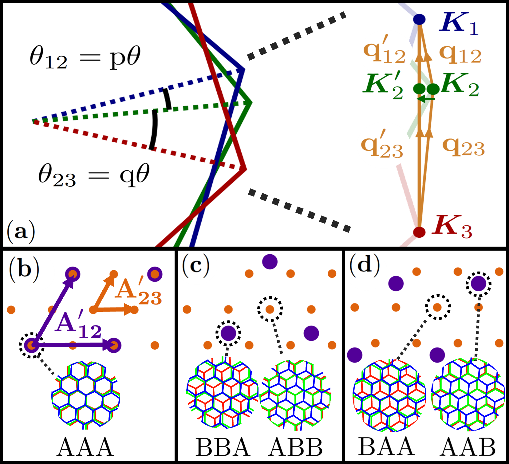
Figure 2: (a, left) The Brillouin zones of the three graphene layers. (a, right) A slight biaxial dilation and twist of the second layer, $\bm{K}_{2}\rightarrow\bm{K}^{\prime}_{2}$, leads to a configuration where $\bm{K}_{1}-\bm{K}^{\prime}_{2}=\mathbf{q}^{\prime}_{12}$ and $\bm{K}^{\prime}_{2}-\bm{K}_{3}=\mathbf{q}^{\prime}_{23}$ are exactly commensurate: $\mathbf{q}^{\prime}_{12}=\frac{\text{p}}{\text{q}}\mathbf{q}^{\prime}_{23}$. Here, we illustrate the $\text{p}/\text{q}=1/2$ case. (b) The commensurate structure at $\mathbf{d}=0$, with the AA stacking regions of layers 1 and 2 in purple, and layers 2 and 3 in orange. The local atomic stacking is illustrated at certain high symmetry points. (c,d) Same as (b) but with a shift of $\mathbf{d}=+\bm{\delta},-\bm{\delta}$ respectively.

We remark that, at this point, the uniform biaxial heterostrain and twist is simply a theoretical tool to construct a commensurate periodic approximant. We do not always expect this kind of deformation to occur in a real system. Nevertheless, the commensurate structure is a good approximation for the local physics at the moiré scale, as the differences only become apparent over distances $\sim|\bm{K}^{\prime}_{2}-\bm{K}_{2}|^{-1}$. This local commensurate description is characterized by the commensurate moiré reciprocal lattice vectors, $\mathbf{G}^{\prime}_{ll^{\prime}}$, and the relative displacement between the two moiré lattices $\mathbf{d}$. Explicitly, if we fix some reference point of a given trilayer lattice structure, and define $\mathbf{d}_{t}$ as the distance from that point to a nearby AA region of layers 1 and 2, and $\mathbf{d}_{b}$ as the distance to a nearby AA region layers 2 and 3, then we can define

$$\mathbf{d}=|\text{p}\text{q}|(\mathbf{d}_{t}-\mathbf{d}_{b})\mod(\mathbf{A}^{\prime})$$ (1)

which respects the periodicity of the commensurate structure, and is independent of which nearby AA regions are chosen. Clearly, when $\mathbf{d}=0$, each unit cell of the commensurate structure will contain an AAA stacking. When $\mathbf{d}=\pm\bm{\delta}\equiv\pm\mathbf{A}^{\prime}(1/3,1/3)^{T}$ the unit cell will instead contain at least one of an AAB, ABB, BAA, or BBA stacking region.

The value of $\mathbf{d}$ at a point $\mathbf{r}$ can also be directly related to local atomic stacking configurations. Suppose that, at the reference point $\mathbf{r}$, the local atomic positions in layer $l$ appears shifted by $\mathbf{s}_{l}$ relative to that of the origin. Then, the expression for $\mathbf{d}$ is given by (see Appendix for derivation)

$$\mathbf{d}(\mathbf{s}_{1},\mathbf{s}_{2},\mathbf{s}_{3})=\mathbf{A}^{\prime}\left[q\mathbf{A}_{1}^{-1}\mathbf{s}_{1}-(q+p)\mathbf{A}_{2}^{-1}\mathbf{s}_{2}+p\mathbf{A}_{3}^{-1}\mathbf{s}_{3}\right].$$ (2)

With this in mind, we now consider the fully relaxed lattice structure of multi-moiré TTG.

We model lattice relaxation utilizing the configuration space method developed in Zhu et al. [56]. To obtain the relaxation pattern, we minimize the total energy as a function of the relaxation displacement vectors in the local configuration space (see Appendix D for details) [57]. The total energy is a sum of intralayer and interlayer energies. The intralayer energy is the elastic energy cost due to the surface deformation, and the interlayer energy is the energy due to the layer misfit, which is parametrized by the Generalized Stacking Fault energy (GSFE) [58, 59]. Both of these terms can be obtained with first-principles Density Functional Theory [60, 56].

We compute the local shift field $\mathbf{u}_{l}(\mathbf{r})$ for the fully relaxed structure at a variety of twist angles. At a point $\mathbf{r}$, the local atomic positions are shifted by $\mathbf{s}_{l}(\mathbf{r})=-\mathbf{r}+\mathbf{u}_{l}(\mathbf{r})$. Plugging this into Eq. (2) gives an expression for the $\mathbf{d}(\mathbf{r})$ in the relaxed structure as a function of position. The quantity $\mathbf{d}(\mathbf{r})$ should be understood as the following: if we look at the local atomic structure at $\mathbf{r}$ and extend it infinitely into the commensurate structure $\mathbf{A}^{\prime}$, then this structure would be characterized by the constant shift vector $\mathbf{d}(\mathbf{r})$ between the two moiré patterns. In the unrelaxed structure, $\mathbf{s}_{l}(\mathbf{r})=-\mathbf{r}$, and $\mathbf{d}(\mathbf{r})$ varies linearly with $\mathbf{r}$, and is periodic in $\mathbf{r}$ with the supermoiré periodicity $a_{\mathrm{sm}}$. In the presence of lattice relaxation, we expect that $\mathbf{d}(\mathbf{r})$ will exhibit some moiré-scale fluctuations due to lattice relaxation at the moiré scale, but more importantly, it should capture the long wavelength supermoiré scale relaxation. In particular, if the system relaxes into large domains of a commensurate structure, $\mathbf{d}(\mathbf{r})$ should remain roughly constant throughout the entire domain (up to moiré-scale fluctuations).

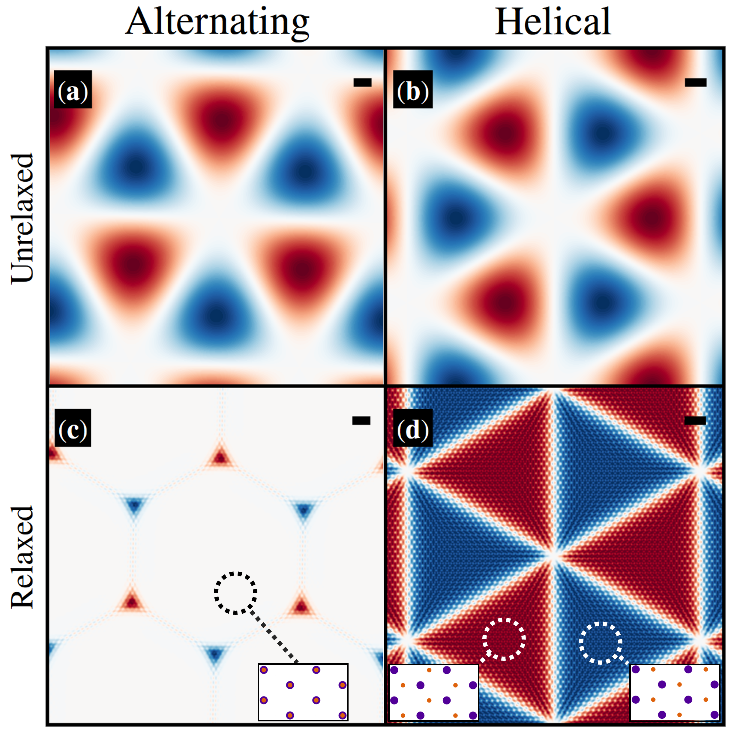
Figure 3: The value of the function, $W(\mathbf{d}(\mathbf{r}))$, for twist angles with $|\theta_{12}/\theta_{23}|\approx 1$. The unrelaxed structure is shown for (a) almost mirror symmetric $(1.60^{\circ},-1.65^{\circ})$-TTG and (b) $(1.85^{\circ},1.85^{\circ})$-TTG. $\mathbf{d}=0$ in the white regions, and $\mathbf{d}=\pm\bm{\delta}$ in the red and blue regions, respectively. The relaxed lattice structures is shown for (c) $(1.60^{\circ},-1.65^{\circ})$-TTG, which forms large domains where $\mathbf{d}=0$, and (d) $(1.85^{\circ},1.85^{\circ})$-TTG, forms large domains where $\mathbf{d}=\pm\bm{\delta}$. Insets show the relative shift of the AA stacking regions of each layer pair, as in Fig. 2. The scale bar is 30nm.

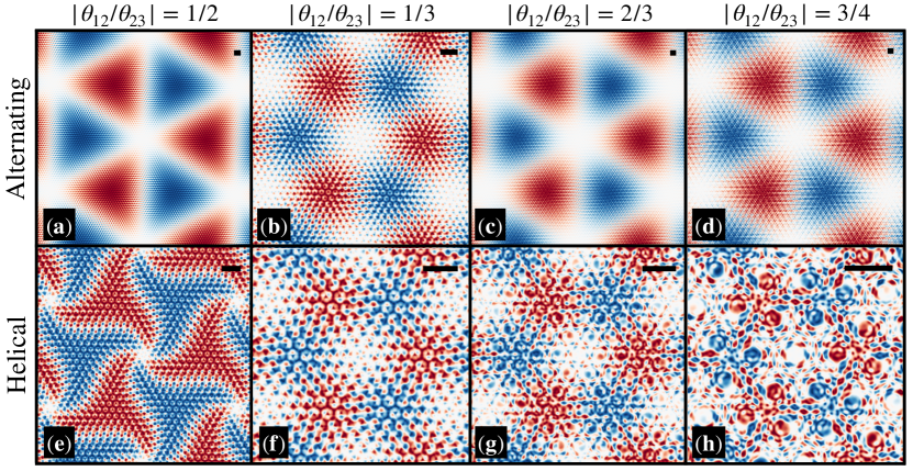
Figure 4: The function $W(\mathbf{d}(\mathbf{r}))$ is plotted for the relaxed lattice structure for alternating ($\theta_{12}/\theta_{23}<0$) and helical ($\theta_{12}/\theta_{23}>0$) TTG near the first magic angles: (a) $(1.30^{\circ},-2.60^{\circ})$, (b) $(1.20^{\circ},-3.60^{\circ})$, (c) $(1.40^{\circ},-2.10^{\circ})$, (d) $(1.50^{\circ},-2.00^{\circ})$, (e) $(1.25^{\circ},2.50^{\circ})$, (f) $(1.20^{\circ},3.60^{\circ})$, (g) $(1.50^{\circ},2.25^{\circ})$, and (h) $(1.60^{\circ},2.13^{\circ})$. The scalebar represents 30nm. Only for helical $\text{p}/q=1/2$ does the structure relax into a polycrystalline structure, with clear blue/red domains forming. For the remaining fractions, the long wavelength behavior resembles that of the unrelaxed case (Fig. 3b).

In Fig. 3, we show how $\mathbf{d}(\mathbf{r})$ behaves for two illustrative examples: almost mirror-symmetric $(1.60^{\circ},-1.65^{\circ})$-TTG and $(1.85^{\circ},1.85^{\circ})$-TTG. Previous studies have shown that $(\theta,-\theta)$-TTG relaxes towards a single-moiré structure with $\mathbf{d}=0$ [61, 62], while $(\theta,\theta)$-TTG relaxes into domains of the single-moiré structure with $\mathbf{d}=\pm\bm{\delta}$ [56, 49, 52]. We plot the function $W(\mathbf{d})=\sum_{j=1,2,3}\sin(\mathbf{g}_{j}^{\prime}\cdot\mathbf{d})$, where $(\mathbf{g}_{1}^{\prime},\mathbf{g}_{2}^{\prime})=\mathbf{G}^{\prime}$ and $\mathbf{g}_{3}^{\prime}=-\mathbf{g}_{1}^{\prime}-\mathbf{g}_{2}^{\prime}$. $W(\mathbf{d})$ is zero when $\mathbf{d}=0$, and approaches its maximum/minimum at $\mathbf{d}=\pm\bm{\delta}$. In the unrelaxed structure, Fig. 3(a,b), $W(\mathbf{d}(\mathbf{r}))$ varies smoothly in space with the supermoiré periodicity, as expected. In the relaxed structure, Fig. 3(c,d), we find $\mathbf{d}(\mathbf{r})$ relaxes strongly to large hexagonal domains with $\mathbf{d}(\mathbf{r})\approx 0$ for alternating TTG, and large triangular domains with $\mathbf{d}(\mathbf{r})\approx\pm\bm{\delta}$ for helical TTG, consistent with earlier findings.

We now proceed to characterize twist angles at other rational fractions $\theta_{12}/\theta_{23}=\text{p}/\text{q}$. For each fraction, we focus on twist angles near the magic angles (determined later in Sec III). Our results for the relaxed structure are shown in Fig. 4, and should be compared to the unrelaxed structure which is identical to Fig. 3b up to an overall rescaling. We highlight several key observations.

For alternating twist angles $\theta_{12}/\theta_{23}<0$ (except for near $\theta_{12}/\theta_{23}=-1$), we find that, despite the very large supermoiré period, the effect of lattice relaxation is weak and $\mathbf{d}(\mathbf{r})$ closely resembles that of the unrelaxed case. This implies that, for alternating twists with $\theta_{12}/\theta_{23}\neq 1$, the interlayer elastic energy gain from forming a locally commensurate structure $\mathbf{A}^{\prime}$ is smaller than the intralayer elastic energy cost required to do so. These findings are surprising, given how strongly the $\theta_{12}/\theta_{23}\approx-1$ case (Fig. 3c) relaxes towards the $\mathbf{d}=0$ structure.

For helical twist angles, $\theta_{12}/\theta_{23}>0$, we find that lattice relaxation has a stronger effect. For $\theta_{12}/\theta_{23}=1/2$, we find domains of commensurate $\mathbf{d}=\pm\bm{\delta}$ regions, separated by a network of curved domain walls. For other fractions $1/3,2/3,$ and $3/4$, we find that relaxation does not result in the formation of large periodic domains, but still leads to visible moiré-scale fluctuations.

Our results demonstrate that lattice relaxation effects are generally more significant for helical twists than alternating twists. Only for the $\theta_{12}/\theta_{23}=\pm 1$, and for the helical $\theta_{12}/\theta_{23}=1/2$, does multi-moiré TTG relax into large domains of a single-moiré structure. This structure, consisting of large domains of roughly constant $\mathbf{d}$ separated by sharp domain boundaries, is reminiscent of a polycrystal, except that different grains have a periodic structure instead of being randomly arranged. We thus refer to these structures as periodic polycrystals . For all other angles, $\mathbf{d}$ varies smoothly in position (up to the moiré-scale fluctuations) similar to the unrelaxed case. This structure is characterized by a set of two incommensurate reciprocal lattice vectors, $\mathbf{G}_{12}$ and $\mathbf{G}_{23}$, and is therefore a moiré quasicrystal [47].

We remark that our conclusions of the relaxed structure will generally depend on magnitude of twist angle, not just their ratio. Our results are valid for twist angles near the first magic angle, which are of most potential interest for strongly correlated physics. At smaller or larger overall twist angles, qualitatively different relaxation patterns can occur. Finally, high resolution images of the moiré AA stacking regions in the relaxed structure are available in the supplemental material.

III Local Hamiltonian and Magic Angles

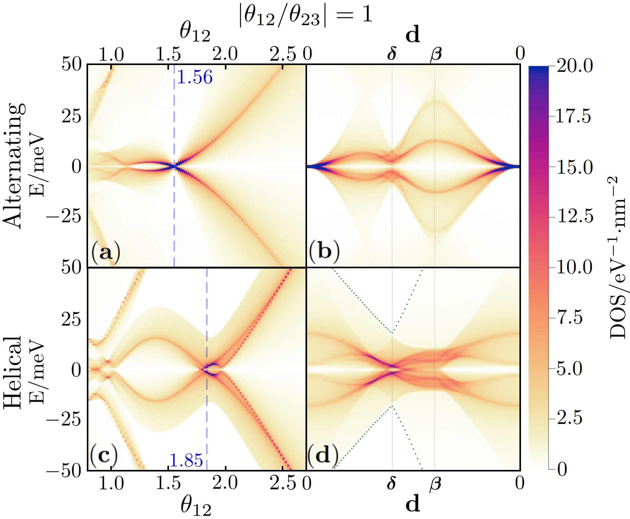
Figure 5: (a,c) The DOS as a function of twist angle, calculated using Eq. (3) for two known cases. (a) twist angles $\theta_{12}=-\theta_{23}$, and shift $\mathbf{d}=0$. (c) twist angles $\theta_{12}=\theta_{23}$, and shift $\mathbf{d}=\bm{\delta}$. The magic angles of $1.56^{\circ}$ and $1.85^{\circ}$ where the DOS is peaked (dashed line) correspond to magic angles of Refs. 32, 33, 34, 35, 36, 38 and 48 respectively. (b,d) The DOS at the magic angle as a function of moiré shift, using the path described in Fig. 7(b).

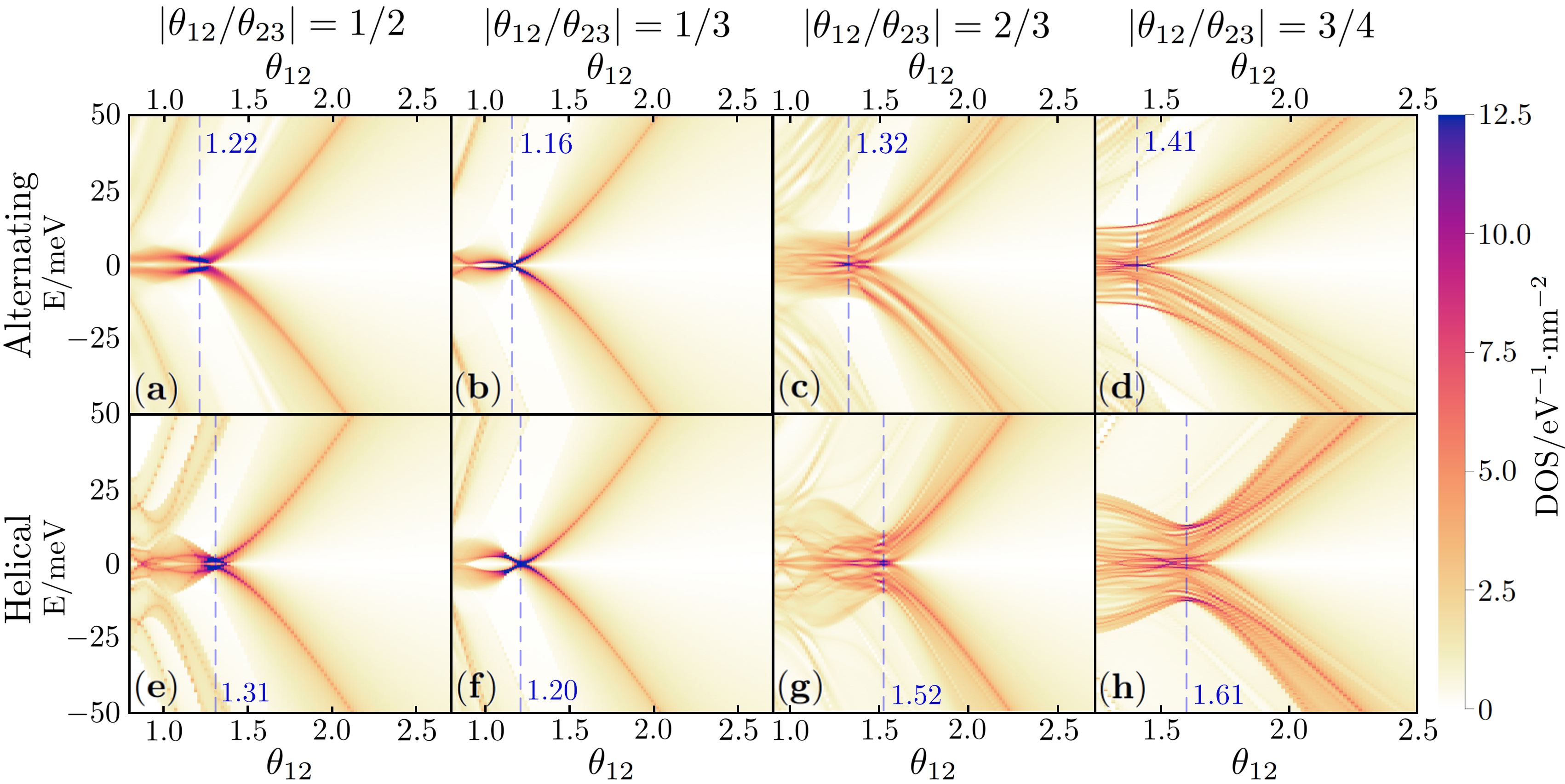
Figure 6: The local DOS calculated as a function of twist angle, $\theta_{12}=\frac{\text{p}}{\text{q}}\theta_{23}$, calculated using Eq. (3). (e) Helical $1/2$ is a periodic polycrystal, so the dominant shift of $\mathbf{d}=\bm{\delta}$ was used. (a-d,f-h) For the remaining structures, the DOS is averaged over all shifts. The magic angle where the DOS is peaked is estimated with a dashed blue line. The peaks of the DOS have a width of $\sim.1^{\circ}$.

In this section, we will consider the electronic structure of multi-moiré TTG. Following our discussion in Sec. II, we treat local moiré scale lattice structure of multi-moiré TTG as two commensurate moiré lattices with a relative shift between them. Such a system is described by a generalized Bistritzer-MacDonald model [64, 54, 49, 55, 65]. The Hamiltonian for the K-valley is

$$H=\begin{pmatrix}-iv_{F}\bm{\sigma}_{\theta_{12}}\cdot\bm{\nabla}&T_{12}(\mathbf{r}-\mathbf{d}_{t})&0\\ T_{12}^{\dagger}(\mathbf{r}-\mathbf{d}_{t})&-iv_{F}\bm{\sigma}\cdot\bm{\nabla}&T_{23}(\mathbf{r}-\mathbf{d}_{b})\\ 0&T_{23}^{\dagger}(\mathbf{r}-\mathbf{d}_{b})&-iv_{F}\bm{\sigma}_{-\theta_{23}}\cdot\bm{\nabla}\end{pmatrix}$$ (3)

where $\bm{\sigma}_{\theta}=e^{-i\theta\sigma_{3}/2}(\sigma_{1},\sigma_{2})e^{i\theta\sigma_{3}/2}$, and $\mathbf{d}_{t,d}$ is displacement of the between the top (12) and bottom (23) moiré lattice respectively. In practice, the Pauli rotation simply results in a small particle-hole asymmetry, and so we make the approximation $\bm{\sigma}_{\theta}\approx\bm{\sigma}$. Since a uniform displacement of both moiré lattices is trivial, the spectrum can be parameterized in terms of the shift $\mathbf{d}=|\text{p}\text{q}|(\mathbf{d}_{t}-\mathbf{d}_{d})$. The shift is odd under $C_{2z}\mathcal{T}$ symmetry $\mathbf{d}\rightarrow-\mathbf{d}$ (the product of two-fold rotations, and time-reversal symmetry).

The tunneling matrices between adjacent layers $l$ and $l^{\prime}$ are

$$T_{ll^{\prime}}(\mathbf{r}) =w\sum_{n=0}^{2}e^{i\mathbf{q}^{\prime}_{n,ll^{\prime}}\cdot\mathbf{r}}T^{n}$$ (4a)

$$T^{n-1} =\kappa\sigma_{3}+\cos(2\pi n/3)\sigma_{1}+\sin(2\pi n/3)\sigma_{2}$$ (4b)

where $\mathbf{q}^{\prime}_{n,ll^{\prime}}$ are the associated tunneling wavevectors, satisfying $(\mathbf{q}^{\prime}_{n,ll^{\prime}})_{x}+i(\mathbf{q}^{\prime}_{n,ll^{\prime}})_{y}=-ik^{\prime}_{\theta_{ll^{\prime}}}e^{-i\frac{2\pi}{3}(n-1)}$, $k^{\prime}_{\theta_{12}}=|\mathbf{K}_{1}-\mathbf{K}^{\prime}_{2}|$ and $k^{\prime}_{\theta_{23}}=|\mathbf{K}^{\prime}_{2}-\mathbf{K}_{3}|$. As before, $\mathbf{K}^{\prime}_{2}$ is defined as in Appendix A. The chiral ratio, $\kappa$, suppresses intra-sublattice tunneling due to lattice relaxation and renormalization; we take $\kappa=0.7$, as many TBG studies indicate that it lies somewhere in the range 0.5–0.8 [66, 67, 60, 68, 69, 70, 71, 72, 73, 74].

We take $\mathbf{q}^{\prime}_{n,ll^{\prime}}$ to be constant in space, but allow for $\mathbf{d}$ to be spatially dependent, reflecting the super-moiré structure of the relaxed lattice [75, 76]. In principle, the spatially variation of $\mathbf{d}$ can be directly included in Eq. (3) by assuming a functional form of $\mathbf{d}(\mathbf{r})$ with a commensurate supermoiré periodicity (this may lead to an effectively periodic supermoiré low-energy continuum model when the Dirac points of the moiré bands are dispersive, but fails when moiré bands are extremely flat like at the first magic angle [53]). The main effect of incorporating the full $\mathbf{d}(\mathbf{r})$ will be to open mini-gaps in the spectrum, while greatly increasing the computational complexity of diagonalizing the Hamiltonian for large supermoiré periods. These mini-gaps reflect wavefunction coherence over the supermoiré scale (several hundred nanometers) and are unlikely to be experimentally relevant in the presence of thermal or disorder effects (except possibly at larger angles, beyond those studied here, where the supermoiré period becomes smaller [77]) We therefore fix $\mathbf{d}$ and treat Eq. (3) as a local Hamiltonian that describes the moiré scale physics in a given region of the full trilayer system.

We use the parameters $v_{F}=8.8\times 10^{5}\,\text{m/s}$ and tunneling energy $w=110\,\text{meV}$ [1]. In Fig. 5 we plot the DOS as a function of $\theta_{12}$ for $\theta_{12}/\theta_{23}=-1$ with shift $\mathbf{d}=0$ and $\theta_{12}/\theta_{23}=1$ with shifts $\mathbf{d}=\bm{\delta}$ (since $\mathbf{d}\rightarrow-\mathbf{d}$ under $C_{2z}\mathcal{T}$, the DOS for $\mathbf{d}=-\bm{\delta}$ is the same). As discussed in Sec. II, these shifts are strongly preferred for these twist angle configurations. We find magic angles of $1.85^{\circ}$ and $1.56^{\circ}$ respectively, in good agreement with experimental values [32, 33, 34, 35, 36, 38, 48].

For the other angle ratios, we first consider the DOS as a function of twist angle. For $\theta_{12}/\theta_{23}=1/2$, lattice relaxation results in the formation of domains with $\mathbf{d}=\pm\bm{\delta}$, and so we calculate the DOS for fixed $\mathbf{d}=\bm{\delta}$. For other p and q, the shift varies smoothly over the super-moiré scale, such that there is no preferred shift. For these systems, we calculate the DOS averaged over all possible $\mathbf{d}$. For all cases, we estimate magic angles as the location where the DOS is most peaked near $E=0$.

To understand the local physics of TTG at these magic angles, we also calculate the DOS as a function of shift at the magic angle indicated in Fig. 6. Since the supermoiré structure enters the local Hamiltonian through the shift, the DOS as a function of shift indicates how the local DOS varies on the supermoiré scale at a fixed twist angle. The DOS as a function of shift at the magic angle is shown in Fig. 7. In Appendix B we also plot the band structure at the magic angle for both $\mathbf{d}=0$ and $\mathbf{d}=\bm{\delta}$. Similar to $\text{p}/\text{q}=1$ TTG, we find gaps where the DOS vanishes above and below the central bands for $\text{p}/\text{q}=\pm 1/2$ and $\text{p}/\text{q}=-1/3$. These gaps are necessarily close when $\mathbf{d}=0$ [24], and only exist near $\mathbf{d}=\pm\bm{\delta}$.

IV Discussion

Having presented both the lattice relaxation and electronic structure of multi-moiré twisted trilayer graphene, we now discuss our results and their physical consequences. We found that, near the first magic angle, only for $\theta_{12}/\theta_{23}\approx\pm 1$ and $1/2$ does the relaxed lattice have a periodic polycrystalline structure, consisting of large domains with a constant shift $\mathbf{d}$. For all other simple rational fractions, $-1/2,\pm 1/3,\pm 2/3,$ and $\pm 3/4$, the supermoiré structure of $\mathbf{d}(\mathbf{r})$ is smoothly varying, closely resembling that of the unrelaxed structure. These structures are therefore quasicrystalline, and do not relax towards a commensurate structure. This quasiperiodicity was assumed in the theoretical analysis of $(1.4^{\circ},-1.9^{\circ})$-TTG in Ref [47] (which is close to $-3/4$), and our full lattice relaxation result confirms this.

These relaxation patterns have important implications for the electronic properties, especially for the potential realization of strongly correlated states. For twist angles in the periodic polycrystalline regime, the “commensurate approximation” from Sec II is physical, and the system relaxes to the locally periodic structure. For these systems, we determined the magic angle at which the DOS is maximized within the dominant domains. At this magic angle, polycrystalline TTG should consist of large regions with a strongly peaked DOS separated by domain walls where the DOS is lower. This will lead to a tendency for such materials to nucleate strongly correlated states within the domains. If the same correlated state can be nucleated in all domains, then proximity effects may effectively wash out the domain walls, as likely occurs in $\theta_{12}/\theta_{23}\approx-1$-TTG where large $\mathbf{d}=0$ domains form (Fig. 3c). However, if the correlated states in adjacent domains have different topology, the domain walls will support gapless modes, leading to network model-like physics. This is believed to occur in ($1.85^{\circ},1.85^{\circ}$)-TTG [48, 49, 50], where symmetry-breaking phases with different Chern numbers form within the $\mathbf{d}=\bm{\delta}$ and $-\bm{\delta}$ domains.

Away from $\theta_{12}/\theta_{23}=\pm 1,1/2$, the domain walls broaden, and the system becomes less like a periodic polycrystal and more like a quasicrystal, with the relative shift smoothly changing over the supermoiré scale. For these cases, we determine the magic angle from the peak in the DOS averaged over $\mathbf{d}$. Compared to $\theta_{12}/\theta_{23}=\pm 1$, Fig. 7 shows that the DOS varies less as a function of the shift in the quasi crystalline regime, and exhibits a peak for all $\mathbf{d}$. This implies that, remarkably, the DOS is still peaked everywhere in space at the magic angle. This should promote the creation of uniform phases, as opposed to the nucleation of local phases, although the nature of these phases may be more complicated due to quasiperiodicity. We speculate that the manifest quasiperiodic nature of the lattice at large p and q may be detrimental to phases with momentum dependence, like charge density waves or non-s-wave superconductivity. The DOS for certain fractions also show gaps opening near $\mathbf{d}=\pm\bm{\delta}$, that close for the values of the shift (this is most pronounced in the band structures, shown in Fig. 8, where a topological gap opens between the central flat bands and remote bands). If the chemical potential is in one of these gaps, the system will be gapped in the $\mathbf{d}=\pm\bm{\delta}$ regions of the relaxed structure, and a network of gapless modes will flow around them. In general, any “domain walls” in the quasicrystal regime will be wide, and may therefore prefer valley-Chern or spin-Chern number changes to Chern number changes [78].

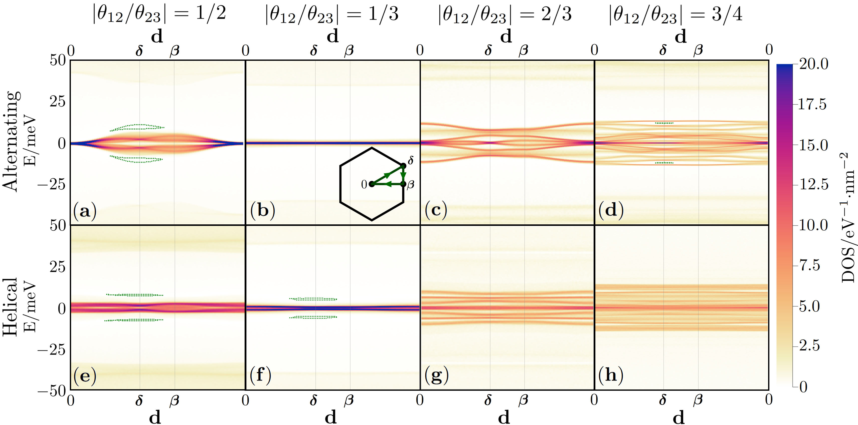
Figure 7: The DOS as a function of shift, $\mathbf{d}$ calculated at the magic angles shown in Table. 1 and Fig. 6. The path taken in real space is given in the inset to (b). Dashed lines illustrate regions where the DOS is zero, indicating a full gap.

In the limit where $\theta_{12}/\theta_{23}\rightarrow 0$, the quasicrystalline nature of the relaxed lattice becomes inconsequential at the first magic angle. This feature can be understood by the fact that when the second and third graphene layers have a large twist angle, they are effectively electronically decoupled from each other. Ref. 46 studied a trilayer graphene device at twist angles $\sim(1.1^{\circ},-5.5^{\circ})$ and showed that the third layer effectively behaved as a decoupled monolayer, while the first and second layers behaved as MATBG. In Table 1, we find that for $\theta_{12}/\theta_{23}=1/\text{q}$, $\theta_{12}$ approaches the bilayer graphene magic angle as $|q|$ increases, with $\theta_{12}\approx 1.1^{\circ}$ for $|q|=4$. We can understand this as the effective twist decoupling of the third layer. Any correlated physics in this regime should match that of MATBG, with possible screening effects from the decoupled monolayer graphene. The addition of the additional monolayer graphene can also change the global symmetry of the system, but given the electronic decoupling, this explicit symmetry breaking is unlikely to be consequential.

It is worth commenting on the possible connection between the $\theta_{12}/\theta_{23}=-3/4$ TTG and the experimental observation of strongly correlated physics in the $\sim(1.4^{\circ},-1.9^{\circ})$ MQC [47]. Remarkably, our analysis suggests that $(1.4^{\circ},-1.9^{\circ})$ is close to precisely the magic angle of the $-3/4$ TTG system. The lattice relaxation calculations show a quasicystalline super-moiré structure. The high DOS (Fig. 7) could also lead to flavor polarization and superconductivity observed in hole doped MQC. However, at charge neutrality, the MQC displays quantum oscillations that are well described by dispersive Dirac cones. These Dirac cones are not present in the local band structure of magic angle $-3/4$ TTG calculated in this work, as shown in Fig. 8. A possible resolution to this is that the Dirac velocity at the magic angle is significantly renormalized[79, 80, 81, 82] at charge neutrality, effectively making the flat bands Dirac-like. The increased DOS at the magic angle therefore either induces a correlated phase or renormalizes the system to have Dirac-like bands, depending on the filling. This possibility motivates the experimental study of $-3/4$ TTG at other twist angles, to determine whether strongly correlated physics only appears at our predicted magic angle of $(1.41^{\circ},-1.88^{\circ})$, or whether it appears more generically.

In this work we have focused on the properties of multi-moiré TTG near twist angles with simple fractions $\theta_{12}/\theta_{23}=\text{p}/\text{q}$ in order to probe the tendency to relax into exactly commensurate structures. However, our results apply more generally. Ultimately, the DOS is a physical quantity which should depend smoothly on the twist angles. Angles that lie on the magic line in Fig. 1 will have a high DOS, even if they are not exactly rational. Our conclusions of the relaxed lattice structure will also depend smoothly on the twist angles. We therefore conclude that all along the magic line, multi-moiré TTG will consist of regions where the relaxed lattice structure is a quasicrystal, with small regions near $(1.56^{\circ},-1.56^{\circ})$, $(1.85^{\circ},1.85^{\circ})$, and $(1.31^{\circ},2.61^{\circ})$ where the relaxed lattice structure is a periodic polycrystal, and twist decoupling in the large $\theta_{23}$ limit. Notably, the periodic polycrystals are stable to small changes in the twist angle — the main effect of a small twist detuning will merely affect size of the domains [52, 49, 48]. Thus, the behaviors identified in this work are therefore not tied to specific rational twist angles, but are part of a continuum of TTG systems along a magic line.

Our results have important implications for future experiments. Our results for the relaxed structure, in particular the formation or non-formation of commensurate domains, can be readily probed by imaging techniques such as atomic force microscopy or scanning tunneling microscopy (STM). STM can also directly probe the local DOS as a function of position; for quasicrystalline structures, $\mathbf{d}$ varies smoothly in space and our DOS results shown in Fig. 7 directly reflects the supermoiré scale spatial dependence of the local DOS. For twist angles where the supermoiré periods are very large, on the order of hundreds of nanometers, techniques such as scanning single-electron transistor or microwave impedance microscopy can detect the supermoiré scale spatial variations in the electronic properties. In transport, we predict that correlated behaviors are likely to appear along a magic line where the DOS is maximized. This physics may manifest in a variety of different ways: correlated insulators, orbital ferromagnetism, anomalous Hall effects, or superconductivity, to name some possibilities. The broad variety of physics already observed in experiments [30, 31, 32, 33, 34, 35, 36, 47, 46, 48] is evidence of the wide range of possibilities in this platform. The precise nature of the correlated physics that will appear in each system along the magic line is an interesting open question for future theoretical and experimental studies.

In summary, we have investigated the lattice and electronic properties of multi-moiré TTG near the first magic angles. The combined results of our analysis of the lattice relaxation and electronic properties of multi-moiré TTG reveals a rich phase diagram of polycrystalline and quasicrystalline structures along a magic line of twist angles where the DOS is sharply peaked, summarized in Fig. 1. At these twist angles, we predict the realization of strongly correlated physics. Many interesting strongly correlated phenomena have already been observed in multi-moiré TTG systems (Table 1); however, the full phase space is only just beginning to be explored. Our study sets the stage for future theoretical and experimental exploration of the full phase space of multi-moiré TTG.

Appendix A Local Commensuration

We denote the lattice vectors for individual layers as $\mathbf{A}_{l}$, the moiré lattice as $\mathbf{A}_{ll^{\prime}}$ and the moire-of-moire lattice vectors as $\mathbf{A}$. The corresponding reciprocal lattice vectors are $\mathbf{G}_{l}$, $\mathbf{G}_{ll^{\prime}}$ and $\mathbf{G}$. Primed vectors denote the distorted, commensurate vectors. These will denote the matrices $\mathbf{G}_{l}=[\mathbf{g}_{1,l},\mathbf{g}_{2,l}]=[\mathbf{g}_{1,l},\mathbf{R}(2\pi/3)\mathbf{g}_{1,l}]$, and so forth, where $\mathbf{R}(\theta)$ is a rotation matrix.

If we wish to enforce global commensuration

$$\text{q}\mathbf{G}_{12}^{\prime}=\text{p}\mathbf{G}_{23}^{\prime}$$ (5)

we can fix two of the layers and distort the third. We choose to distort the second layer as it is the most symmetric distortion. We do so by using the fact that the moiré reciprocal vectors can be written in terms of the layer lattice vectors

$$\mathbf{G}_{ll^{\prime}}=\mathbf{G}_{l^{\prime}}-\mathbf{G}_{l}$$ (6)

Since $\mathbf{g}_{2,ll^{\prime}},\mathbf{g}_{2,l}$ can be written as an appropriate rotation of $\mathbf{g}_{1,ll^{\prime}},\mathbf{g}_{1,l}$, we can distort the second layer in a way that preserves its hexagonal symmetry. This particular distortion is given by the condition

$$\mathbf{G}_{2}^{\prime}=\frac{\text{q}}{\text{p}+\text{q}}\mathbf{G}_{1}+\frac{\text{p}}{\text{p}+\text{q}}\mathbf{G}_{3}$$ (7)

which gives us additionally our hopping wavevectors and our supermoiré reciprocal vectors

$$\mathbf{G}_{12}^{\prime} =\frac{\text{p}}{\text{p}+\text{q}}(\mathbf{G}_{3}-\mathbf{G}_{1})$$ (8a)

$$\mathbf{G}_{23}^{\prime} =\frac{\text{q}}{\text{p}+\text{q}}(\mathbf{G}_{3}-\mathbf{G}_{1})$$ (8b)

$$\mathbf{G}^{\prime} =\frac{1}{p+q}(\mathbf{G}_{3}-\mathbf{G}_{1})$$ (8c)

We visualize this distortion as shifting the $\bm{K}_{2}$ point onto the line connecting $\bm{K}_{1}$ to $\bm{K}_{3}$, as seen in Fig. 2. Naturally, Eqs. 8 diverge for (p,q)=(1,-1), but since the moiré lattices are already exactly commensurate, we don’t need to use this procedure. These reciprocal vectors encode everything about the geometry of the system, and all computations are done in terms of these reciprocal vectors. From these distorted reciprocal vectors, the distorted real space lattice vectors can be calculated

$$\mathbf{A}_{l}^{\prime}=2\pi[(\mathbf{G}_{l}^{\prime})^{\intercal}]^{-1}$$ (9a)

$$\mathbf{A}_{ll^{\prime}}^{\prime}=2\pi[(\mathbf{G}_{ll^{\prime}}^{\prime})^{\intercal}]^{-1}$$ (9b)

$$\mathbf{A}^{\prime}=2\pi[(\mathbf{G}^{\prime})^{\intercal}]^{-1}$$ (9c)

Since it is shared in both moiré BZs, we fix $\mathbf{K}_{2}^{\prime}$ at the centre of the supermoiré BZ, $\gamma$, and position $\mathbf{K}_{1}=\mathbf{K}_{2}^{\prime}+\mathbf{q}^{\prime}_{1,12}$ and $\mathbf{K}_{3}=\mathbf{K}_{2}^{\prime}-\mathbf{q}_{1,23}^{\prime}$ accordingly. Since we enforce exact commensuration, these will fold onto one of the high symmetry points $\gamma$, $\kappa$, $\kappa^{\prime}$, depending on the exact structure. Since we neglect Pauli rotation of the Dirac cones, we ensure that the reciprocal vector $\mathbf{G}^{\prime}$ is exactly aligned with the coordinate axis, which maintains exact particle-hole symmetry of the DOS.

Appendix B Magic Angle Band Structures

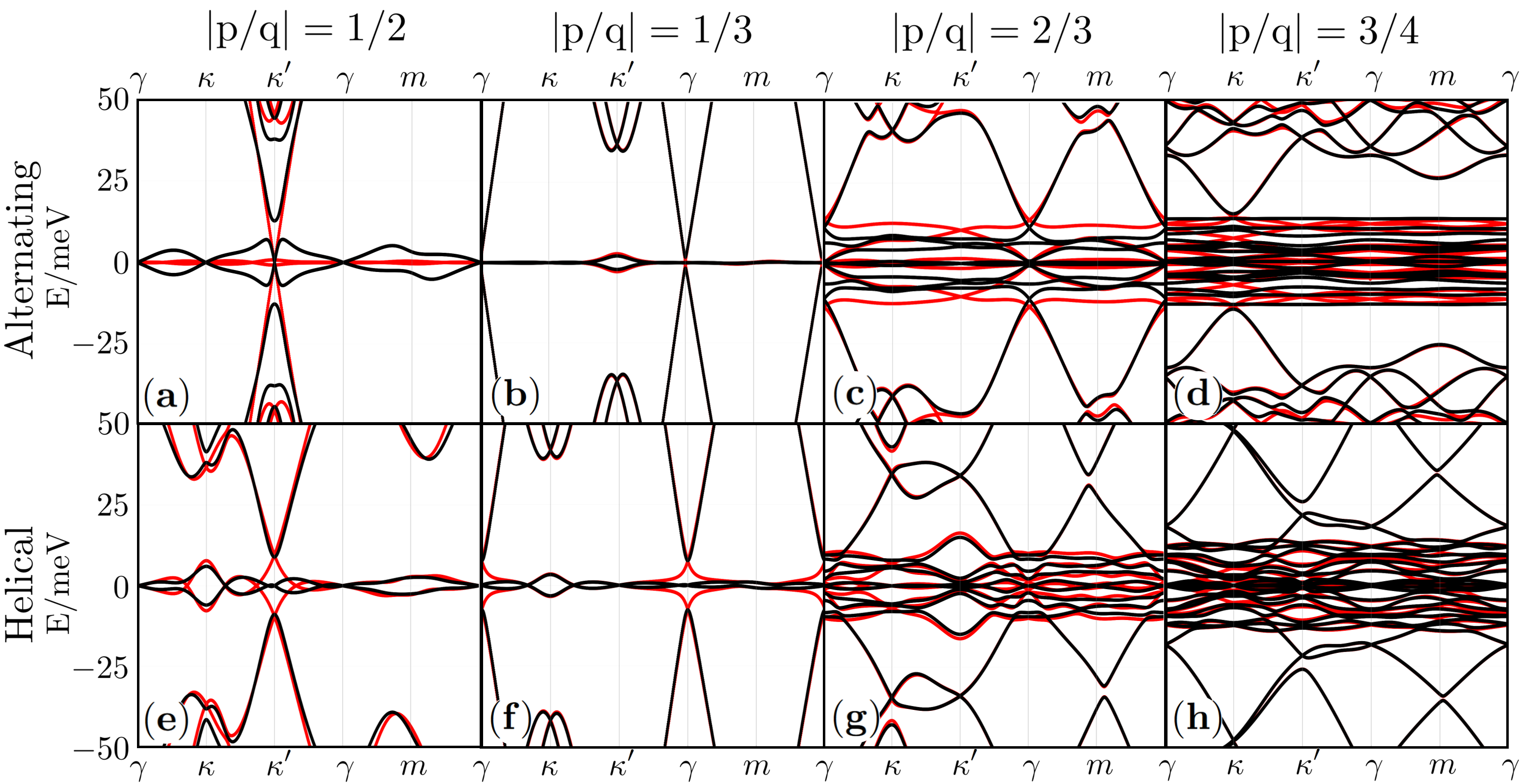
Figure 8: Band structures near magic angles for selected configurations. The black bands represent the shift $\mathbf{d}=\bm{\delta}$, while the red bands represent the shift $\mathbf{d}=0$ Note that in (a,e, f) that the central bands are gapped at $\mathbf{d}=\bm{\delta}$, as illustrated in Fig. 7.

We begin with Eq. (3), dropping the Pauli rotation ($\bm{\sigma}_{\theta}\to\bm{\sigma}$). We apply a unitary transformation to shift the tunneling wavevectors by $-\mathbf{q}_{0,ll^{\prime}}^{\prime}$, so that we may transform

$$\mathbf{q}_{0,ll^{\prime}}^{\prime},\mathbf{q}_{1,ll^{\prime}}^{\prime},\mathbf{q}_{2,ll^{\prime}}^{\prime}\longrightarrow 0,-\mathbf{g}_{1,ll^{\prime}}^{\prime},\mathbf{g}_{2,ll^{\prime}}^{\prime}$$ (10)

explicitly, this unitary for shifting $\text{q}^{\prime}_{n,ll^{\prime}}$ is given

$$U_{12} =\begin{pmatrix}e^{-i\mathbf{q}^{\prime}_{0,12}\cdot\mathbf{r}}&0&0\\ 0&e^{i\mathbf{q}^{\prime}_{0,12}\cdot\mathbf{r}}&0\\ 0&0&1\end{pmatrix}$$ (11a)

$$U_{23} =\begin{pmatrix}1&0&0\\ 0&e^{-i\mathbf{q}^{\prime}_{0,23}\cdot\mathbf{r}}&0\\ 0&0&e^{i\mathbf{q}^{\prime}_{0,23}\cdot\mathbf{r}}\\ \end{pmatrix}$$ (11b)

so that

$$U_{12}U_{23}H_{\bm{K}}U_{23}^{\dagger}U_{12}^{\dagger}=\begin{pmatrix}-iv_{F}\bm{\sigma}\cdot(\bm{\nabla}-\bm{K}_{1})&T_{12}(\mathbf{r}-\mathbf{d}_{t})e^{-i\mathbf{q}^{\prime}_{0,12}}&0\\ T^{\dagger}_{12}(\mathbf{r}-\mathbf{d}_{t})e^{i\mathbf{q}^{\prime}_{0,12}}&-iv_{F}\bm{\sigma}\cdot(\bm{\nabla}-\bm{K}_{2})&T_{23}(\mathbf{r}-\mathbf{d}_{b})e^{-i\mathbf{q}^{\prime}_{0,23}}\\ 0&T^{\dagger}_{23}(\mathbf{r}-\mathbf{d}_{b})e^{i\mathbf{q}^{\prime}_{0,23}}&-iv_{F}\bm{\sigma}\cdot(\bm{\nabla}-\bm{K}_{3})\end{pmatrix}$$ (12)

The unitaries also affect the diagonal kinetic terms as a momentum shift. Then, we can rewrite

$$\tilde{T}_{ll^{\prime}}(\mathbf{r})=w\sum_{n=0}^{2}e^{i\mathbf{g}^{\prime}_{n,ll^{\prime}}\cdot\mathbf{r}}T^{n}$$ (13)

where we define $\mathbf{g}^{\prime}_{0,ll^{\prime}}=0$ for convenience. The wavefunctions of the transformed Hamiltonian satisfies the Bloch periodicity

$$\psi^{\prime}_{\mathbf{k}}(\mathbf{r}+\mathbf{a})=e^{i\mathbf{k}\cdot\mathbf{a}}\psi^{\prime}_{\mathbf{k}}(\mathbf{r})$$ (14)

Since we have approximated our moiré lattices to be exactly commensurate, this allows us to define a unified BZ that is labelled by the momenta of all layers simultaneously.

Thus, we choose as a basis planewave states $\lvert\mathbf{k},l,\tau\rangle$ labeled by crystal momentum $\mathbf{k}$, layer $l$, and sublattice $\tau$. These satisfy

$$\langle\mathbf{r}|\mathbf{k},l,\tau\rangle=e^{i\mathbf{k}\cdot\mathbf{r}}\lvert l,\tau\rangle$$ (15)

so

$$\langle\mathbf{r}\rvert e^{i\mathbf{q}\cdot\mathbf{r}}\lvert\mathbf{k},l,\tau\rangle=e^{i(\mathbf{k}+\mathbf{q})\cdot\mathbf{r}}\lvert l,\tau\rangle=\langle\mathbf{r}|\mathbf{k}+\mathbf{q},l,\tau\rangle$$ (16)

Thus, we see that multiplying by a planewave serves to couple different $\mathbf{k}$ modes; this is the effect of the operator $e^{i\mathbf{g}_{n,ll^{\prime}}^{\prime}\cdot\mathbf{r}}$ in the expression for $\tilde{T}_{ll^{\prime}}$.

In this basis, the Hamiltonian has layer block-diagonal entries

$$\langle\mathbf{k},l,\tau\rvert H_{\bm{K}}\lvert\mathbf{k},l,\tau^{\prime}\rangle=v_{F}\left[\sigma\cdot(\mathbf{k}-\bm{K}_{l})\right]_{\tau\tau^{\prime}}$$ (17)

and off-diagonal blocks

$$\langle\mathbf{k},l,\tau\rvert H_{\mathbf{K}}\lvert\mathbf{k}^{\prime},l^{\prime},\tau^{\prime}\rangle=\sum_{n=0,1,2}\sum_{\xi=\pm 1}\delta_{\mathbf{k}^{\prime},\mathbf{k}+\mathbf{g}_{n,ll^{\prime}}^{\prime}}we^{i\xi\mathbf{g}_{n,ll^{\prime}}^{\prime}\cdot\mathbf{d}_{ll^{\prime}}}T^{n}_{\tau\tau^{\prime}}\delta_{l^{\prime},l+\xi}$$ (18)

where we define for convenience $g_{n,ll^{\prime}}^{\prime}=-g_{n,l^{\prime}l}^{\prime}$ and $d_{ll^{\prime}}=-d_{ll^{\prime}}$, and we have rewritten $d_{12}\equiv d_{t}$ and $d_{23}=d_{b}$.

Using the moiré reciprocal vectors $\mathbf{g}_{n,12}^{\prime},\,\mathbf{g}_{n,23}^{\prime}$ as the new hopping vectors, a $k$-space lattice representing the Hamiltonian and its couplings is constructed out to a cutoff $E/\hbar v_{F}$ which is set to minimize finite size effects while keeping memory usage reasonable. As the energy cutoff $E$ increases, we consider momenta with increasingly higher momenta which couple more weakly to the momenta within the supermoiré BZ. To calculate the band structures, a consistent $E=3000\,\text{meV}$ was used; for the DOS plots, we used a cutoff of $E=3500\,\text{meV}$ for $\lvert\text{p}/\text{q}\rvert=1$, $E=3300\,\text{meV}$ for $\lvert\text{p}/\text{q}\rvert=1/2,\,1/3,\,2/3$, and $E=3000\,\text{meV}$ for $\lvert\text{p}/\text{q}\rvert=3/4$, This Hamiltonian is numerically diagonalized within the supermoiré BZ using the ArnoldiMethod.jl package and using shift-and-invert transformations to target the eigenvalues closest to zero. To highlight the effect of moiré shift on the band structure (or indeed, lack thereof), we plot the band structure at each magic angle for the two high-symmetry shifts ($\mathbf{d}=0,\bm{\delta}$) in Fig. 8.

Appendix C Density of States

The density of states is calculated by randomly sampling the Brillouin zone and finding the energy eigenvalues. These energies are converted to the density of states by using a Gaussian as an approximation for the delta function, setting the standard deviation to be the same as the width of the energy bins plotted. The density of states is normalized by the area of the supermoiré unit cell. For example, in (1,q) structures, filling the two flat bands represents eight electrons in the moiré unit cell of the smaller angle, or in $\text{q}^{2}$ moiré unit cells of the larger angle. The magic angle is obtained by plotting the density of states against the smaller twist angle, and extracting the angle where the bands are most constricted and show the greatest density of states near $E=0$. For structures that show strong relaxation, we compute the density of states by fixing the shift to be the dominant shift of the relaxed domains. For structures with weaker relaxation, we randomly sample the shifts in addition to the momenta to build up an averaged density of states.

Similarly, we plot the density of states as a function of moiré shifts to illuminate the effects of the spatially varying shift on the local density of states. We plot the density of states as slices along a real space path. Since approximating the delta functions as a Gaussian blurs the boundaries for gap openings, we set a small cutoff $\sim 10^{-4}-10^{-8}\,\text{eV}^{-1}\cdot\text{nm}^{-2}$ below which we consider to be a gap. As seen in the black band structures in Fig. 8(a,e,f), these regions do indicate true gap openings.

Appendix D Configuration space continuum model for relaxation patterns

To calculate the atomic relaxation pattern, we employ a continuum relaxation model in local configuration space [56]. In twisted trilayer graphene with two independent twist angles, there does not exist a largest length scale and the system is incommensurate [56]. Therefore, instead of formulating the problem in real space, we adopt configuration space, which describes the local environment of every position in layer $L_{\ell}$ and bypasses a periodic approximation [57]. Every position in real space $\bm{r}$ in $L_{i}$ can be uniquely parametrized by three shift vectors $\bm{b}^{i\rightarrow j}$ for $j=1,2,3$ that describes the relative position between a given point $\bm{r}$ with respect to all three layers. Note that $\bm{b}^{i\rightarrow j}=\bm{0}$ if $i=j$ since the separation between a position with itself is 0, which leads to a four-dimensional configuration space.

For a given real space position $\bm{r}$, the following linear transformation relates $\bm{r}$ and $\bm{b}^{i\rightarrow j}$ in layer $i$ with respect to layer $j$, and the following linear transformation maps the relaxation from the local configuration to the real space position $\bm{r}$:

$$\bm{b}^{i\rightarrow j}(\bm{r})=(E_{j}^{-1}E_{i}-\mathbb{1})\bm{r},$$ (19)

where $E_{i}$ and $E_{j}$ are the unit cell vectors of layers $i$ and $j$ respectively, rotated by $\theta_{ij}$. In the trilayer system, there is no simple linear transformation between real and configuration space. The relation between the displacement field defined in real space, $\bm{U}^{(i)}(\bm{r})$, and in configuration space, $\bm{u}^{(i)}(\bm{b})$, can be found by evaluating $\bm{u}^{(j)}(\bm{b})$ at the corresponding $\bm{b}^{i\rightarrow j}(\bm{r})$ and $\bm{b}^{i\rightarrow k}(\bm{r})$ with Eq. (19) to obtain

$$\bm{U}^{(i)}(\bm{r})=\bm{u}^{(i)}(\bm{b}^{i\rightarrow j}(\bm{r}),\bm{b}^{i\rightarrow k}(\bm{r})),$$ (20)

where $j,k\neq i$ and $j<k$.

The relaxed energy has two contributions, intralayer and interlayer energies:

$$E^{\mathrm{tot}}(\bm{u}^{(1)},\bm{u}^{(2)},\bm{u}^{(3)})=E^{\mathrm{intra}}(\bm{u}^{(1)},\bm{u}^{(2)},\bm{u}^{(3)})+E^{\mathrm{inter}}(\bm{u}^{(1)},\bm{u}^{(2)},\bm{u}^{(3)}),$$ (21)

where $\bm{u}^{(\ell)}$ is the relaxation displacement vector in layer $\ell$. To obtain the relaxation pattern, we minimize the total energy with respect to the relaxation displacement vector.

We model the intralayer coupling based on linear elasticity theory:

$$E^{\mathrm{intra}}(\bm{u}^{(1)},\bm{u}^{(2)},\bm{u}^{(3)}) =\sum_{\ell=1}^{3}\int\frac{1}{2}\Big{[}G(\partial_{x}u^{(\ell)}_{x}+\partial_{y}u^{(\ell)}_{y})^{2}$$

$$\ \ \ +K((\partial_{x}u^{(\ell)}_{x}-\partial_{y}u^{(\ell)}_{y})^{2}+(\partial_{x}u^{(\ell)}_{y}+\partial_{y}u^{(\ell)}_{x})^{2})\Big{]}d\bm{b},$$ (22)

where $G$ and $K$ are shear and bulk moduli of monolayer graphene, which we take to be $G=47352\,\mathrm{meV/unit\ cell}$, $K=69518\,\mathrm{meV/unit\ cell}$ [60, 56]. Note that the gradient in Eq. (22) is with respect to the real space position $\bm{r}$.

The interlayer energy accounts for the energy cost of the layer misfit, which is described by the generalized stacking fault energy (GSFE)  [58, 59], obtained using first principles Density Functional Theory (DFT) with the Vienna Ab initio Simulation Package (VASP) [83, 84, 85]. GSFE is the ground state energy as a function of the local stacking with respect to the lowest energy stacking between a bilayer. For bilayer graphene, GSFE is maximized at the AA stacking and minimized at the AB stacking. Letting $\bm{b}=(b_{x},b_{y})$ be the relative stacking between two layers, we define the following vector $\bm{v}=(v,w)\in[0,2\pi]^{2}$:

$$\begin{pmatrix}v\\ w\end{pmatrix}=\frac{2\pi}{a_{0}}\matrixquantity[\sqrt{3}/2&-1/2\\ \sqrt{3}/2&1/2]\begin{pmatrix}b_{x}\\ b_{y}\end{pmatrix},$$ (23)

where $a_{0}=2.4595\text{\AA}$ is the graphene lattice constant. We parametrize the GSFE as follows,

$$V^{\mathrm{GSFE}}_{j\pm}=c_{0}+ c_{1}(\cos v+\cos w+\cos(v+w))$$

$$+ c_{2}(\cos(v+2w)+\cos(v-w)+\cos(2v+w))$$

$$+ c_{3}(\cos(2v)+\cos(2w)+\cos(2v+2w)),$$ (24)

where we take $c_{0}=6.832\,\mathrm{meV/cell}$, $c_{1}=4.064\,\mathrm{meV/cell}$, $c_{2}=-0.374\,\mathrm{meV/cell}$, $c_{3}=-0.0095\,\mathrm{meV/cell}$ [56, 60]. The van der Waals force is implemented through the vdW-DFT method using the SCAN+rVV10 functional [86]. In terms of $V^{\mathrm{GSFE}}_{\ell\pm}$, the total interlayer energy can be expressed as follows:

$$E^{\mathrm{inter}} =\frac{1}{2}\int V^{\mathrm{GSFE}}_{1+}(\bm{B}^{1\rightarrow 2})\,\mathrm{d}\bm{b}+\frac{1}{2}\int\left[V^{\mathrm{GSFE}}_{2-}(\bm{B}^{2\rightarrow 1})+V^{\mathrm{GSFE}}_{2+}(\bm{B}^{2\rightarrow 3})\right]\,\mathrm{d}\bm{b}$$

$$+\frac{1}{2}\int V^{\mathrm{GSFE}}_{3-}(\bm{B}^{3\rightarrow 2})\,\mathrm{d}\bm{b},$$

where $\bm{B}^{i\rightarrow j}=\bm{b}^{i\rightarrow j}+\bm{u}^{(j)}-\bm{u}^{(i)}$ is the relaxation modified local shift vector. Note that we neglect the interlayer coupling between layers 1 and 3. The total energy is obtained by summing over uniformly sampled configuration space. The discretization of the four-dimensional configuration space depends on the twist angle. In general, the larger the moiré of moiré periodicity is, the more dense the sampling needs to be in order to resolve the large scale patterns. For the $(1.60^{\circ},1.65^{\circ})$ case, we choose the discretization to be $54\times 54\times 54\times 54$; and for rest of the cases, we choose $36\times 36\times 36\times 36$.

Appendix E AA stacking regions of the fully relaxed structure

In the main text, we showed the shift vector $\mathbf{d}(\mathbf{r})$ of the relaxed structure. In Figures 9 and 10, we further show the AA stacking regions of the fully relaxed structures, providing more insight into the precise relaxation pattern in each of these structures.

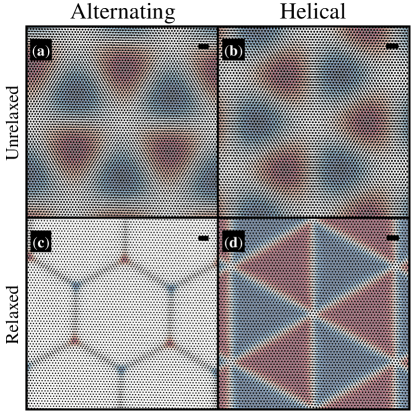
Figure 9: The relaxed structure for the first magic angles are shown, for the case of (a) almost mirror symmetric $(1.60^{\circ},-1.65^{\circ})$-TTG and (b) $(1.85^{\circ},1.85^{\circ})$-TTG. The gray and black dots represent the AA stacking regions of layers 1,2, and layers 2,3, respectively. The function $W(\mathbf{d}(\mathbf{r}))$ from the main text is plotted in the background. The scalebar represents 30nm.

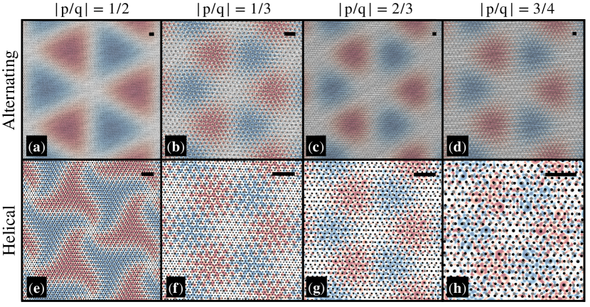
Figure 10: The relaxed structure for the first magic angles are shown, for several rational twist angle configurations. The gray and black dots represent the AA stacking regions of layers 1,2, and layers 2,3, respectively. The function $W(\mathbf{d}(\mathbf{r}))$ from the main text is plotted in the background. The twist angles are (a) $(1.25^{\circ},2.50^{\circ})$, (b) $(1.20^{\circ},3.60^{\circ})$, (c) $(1.50^{\circ},2.25^{\circ})$, (d) $(1.60^{\circ},2.13^{\circ})$, (e) $(1.30^{\circ},-2.60^{\circ})$, (f) $(1.20^{\circ},-3.60^{\circ})$, (g) $(1.40^{\circ},-2.10^{\circ})$, and (h) $(1.50^{\circ},-2.00^{\circ})$. The scalebar represents 30nm.

Appendix F Shift vector derivation

In this section, we derive the expression for the shift vector $\mathbf{d}(\mathbf{s}_{1},\mathbf{s}_{2},\mathbf{s}_{3})$, as a function of the local atomic shifts $\mathbf{s}_{l}$, stated in the main text. For concreteness, let us denote $\mathbf{A}_{0}$ the matrix

$$\mathbf{A}_{0}=a_{0}\begin{pmatrix}1&\frac{1}{2}\\ 0&\frac{\sqrt{3}}{2}\end{pmatrix}$$ (25)

with columns given by the lattice vectors of (untwisted) graphene, and $a_{0}=2.46$Å.

Let us consider a structure in which three layers are rigidly twisted about the origin by angles $\theta_{l}$, and shifted by $\mathbf{s}_{l}$. The lattice vectors of layer $l$ is $\mathbf{A}_{l}=\mathbf{R}(\theta_{l})\mathbf{A}_{0}$, where $\mathbf{R}(\theta)$ is the rotation matrix. Note that $\mathbf{s}_{l}$ is only well defined modulo $\mathbf{A}_{l}$.

Now, suppose that we slightly deform the lattice $\mathbf{A}_{2}\rightarrow\mathbf{A}_{2}^{\prime}$ about the origin. This deformation sends $\mathbf{s}_{2}\rightarrow\mathbf{s}_{2}^{\prime}=\mathbf{A}_{2}^{\prime}\mathbf{A}_{2}^{-1}\mathbf{s}_{2}$. Note that $\mathbf{s}_{2}^{\prime}$ is well defined modulo $\mathbf{A}_{2}^{\prime}$.

After this deformation, the moiré unit cells of layers 1,2, and 2,3, are exactly commensurate. Let us denote the moiré unit vectors

$$\begin{split}\mathbf{A}_{12}^{\prime}=(\mathbf{A}_{1}^{-1}-\mathbf{A}_{2}^{\prime-1})^{-1}\\ \mathbf{A}_{23}^{\prime}=(\mathbf{A}_{2}^{\prime-1}-\mathbf{A}_{3}^{-1})^{-1}\end{split}$$ (26)

which are commensurate with the enlarged unit cell $\mathbf{A}^{\prime}\equiv p\mathbf{A}_{12}^{\prime}=q\mathbf{A}_{23}^{\prime}$.

Let us determine $\mathbf{d}_{12}$, the position of an AA site of layers $1$ and $2$ within the commensurate structure. We define an AA site to be the location where the local shift of the two layers, within their respective unit cells, is identical. At a position $\mathbf{r}$ away from the origin, the local shift appears modified by $-\mathbf{r}$. Thus, $\mathbf{d}_{12}$ is determined by the equation

$$\mathbf{A}_{1}^{-1}(\mathbf{s}_{1}-\mathbf{d}_{12})=\mathbf{A}_{2}^{\prime-1}(\mathbf{s}_{2}^{\prime}-\mathbf{d}_{12})$$ (27)

implying

$$\mathbf{d}_{12}=\mathbf{A}_{12}^{\prime}(\mathbf{A}_{1}^{-1}\mathbf{s}_{1}-\mathbf{A}_{2}^{\prime-1}\mathbf{s}_{2}^{\prime})$$ (28)

which is well-defined modulo the moiré unit vector $\mathbf{A}_{12}^{\prime}$. Similarly, for the second and third layers,

$$\mathbf{d}_{23}=\mathbf{A}_{23}^{\prime}(\mathbf{A}_{2}^{\prime-1}\mathbf{s}_{2}^{\prime}-\mathbf{A}_{3}^{-1}\mathbf{s}_{3})$$ (29)

The relevant parameter in the continuum model of the trilayer is the relative offset of the two moiré AA sites, given by

$$\begin{split}\tilde{\mathbf{d}}=\mathbf{d}_{12}-\mathbf{d}_{23}&=\mathbf{A}_{12}^{\prime}(\mathbf{A}_{1}^{-1}\mathbf{s}_{1}-\mathbf{A}_{2}^{\prime-1}\mathbf{s}_{2}^{\prime})-\mathbf{A}_{23}^{\prime}(\mathbf{A}_{2}^{-1}\mathbf{s}_{2}^{\prime}-\mathbf{A}_{3}^{-1}\mathbf{s}_{3})\\ &=\mathbf{A}^{\prime}\left(\frac{1}{\text{p}}(\mathbf{A}_{1}^{-1}\mathbf{s}_{1}-\mathbf{A}_{2}^{\prime-1}\mathbf{s}_{2}^{\prime})-\frac{1}{\text{q}}(\mathbf{A}_{2}^{-1}\mathbf{s}_{2}^{\prime}-\mathbf{A}_{3}^{-1}\mathbf{s}_{3})\right)\end{split}$$ (30)

However, $\mathbf{d}_{12}$ is equivalent up to a shift by $\mathbf{A}_{12}^{\prime}$, $\mathbf{d}_{12}\cong\mathbf{d}_{12}+\mathbf{A}_{12}^{\prime}\begin{pmatrix}n\\ m\end{pmatrix}$, where $n,m,$ are integers. This implies

$$\tilde{\mathbf{d}}\cong\tilde{\mathbf{d}}+\frac{1}{\text{p}}\mathbf{A}^{\prime}\begin{pmatrix}n\\ m\end{pmatrix}+\frac{1}{\text{q}}\mathbf{A}^{\prime}\begin{pmatrix}n^{\prime}\\ m^{\prime}\end{pmatrix}$$ (31)

Thus, the quantity $\mathbf{d}\equiv|pq|\tilde{\mathbf{d}}$

$$\mathbf{d}\cong\mathbf{d}+\mathbf{A}^{\prime}\begin{pmatrix}qn+pn^{\prime}\\ qm+pm^{\prime}\end{pmatrix}\cong\mathbf{d}+\mathbf{A}^{\prime}\begin{pmatrix}n\\ m\end{pmatrix}$$ (32)

is well-defined modulo the commensurate unit cell $\mathbf{A}^{\prime}$. In the last step, we have used the fact that since p and q are coprime, any integer can be written as an integer multiple $n\text{p}+n^{\prime}\text{q}$. Putting everything together, we have the expression

$$\begin{split}\mathbf{d}(\mathbf{s}_{1},\mathbf{s}_{2},\mathbf{s}_{3})&=\mathbf{A}^{\prime}(q\mathbf{A}_{1}^{-1}\mathbf{s}_{1}-(p+q)\mathbf{A}_{2}^{-1}\mathbf{s}_{2}+p\mathbf{A}_{3}^{-1}\mathbf{s}_{3})\end{split}$$ (33)

as quoted in the main text.