Eureka-Moments in Transformers:
Multi-Step Tasks Reveal Softmax Induced
Optimization Problems

Abstract

In this work, we study rapid, step-wise improvements of the loss in transformers when being confronted with multi-step decision tasks. We found that transformers struggle to learn the intermediate tasks, whereas CNNs have no such issue on the tasks we studied. When transformers learn the intermediate task, they do this rapidly and unexpectedly after both training and validation loss saturated for hundreds of epochs. We call these rapid improvements Eureka-moments, since the transformer appears to suddenly learn a previously incomprehensible task. Similar leaps in performance have become known as Grokking. In contrast to Grokking, for Eureka-moments, both the validation and the training loss saturate before rapidly improving. We trace the problem back to the Softmax function in the self-attention block of transformers and show ways to alleviate the problem. These fixes improve training speed. The improved models reach 95% of the baseline model in just 20% of training steps while having a much higher likelihood to learn the intermediate task, lead to higher final accuracy and are more robust to hyper-parameters.

1 Introduction

A key quality of any intelligent system is its ability to decompose a problem into sub-problems and learn to solve these sub-problems even in the absence of direct feedback. Deep learning has been enabling such capabilities to a certain degree. For example, deep classifiers learn the hierarchical feature representations necessary to build a good classifier. Language models build groups of tokens required to derive the meaning of a token and hence the whole sentence. Reinforcement learning learns object representations required to predict how to receive a sparse reward. While aforementioned examples show great promise, researchers and practitioners invest substantial effort in designing the training process to learn sub-tasks. For instance, reward shaping is a common practice in reinforcement learning and many computer vision works propose explicit or implicit intermediate supervision. At the same time, we are not aware of a study on implicit multi-step learning.

One way to find out more about it could be to study popular tasks, for which many benchmarks and results already exist, in more detail. In fine-grained classification, the network could initially learn super-classes and subsequently refine its classification. In BERT pretraining (Kenton & Toutanova, 2019) the network might first learn word frequencies and only later learns to use the context. Indeed, RoBERTa seems to learn these tasks consecutively and improves on the second task rapidly after an early saturation phase (Fig. 1(c)). However, real data prohibits a clean study: 1) The exact sub-tasks are typically unknown and, hence, are hard to study. 2) Not all samples may require multi-step reasoning and there could be many learning shortcuts (Geirhos et al., 2020), making progress on the multi-step task unrecognizable. 3) The features necessary for the tasks are unknown, i.e. we cannot study what the network fails to learn, let alone the reason for it. 4) Even the number of steps is unknown, thus, we cannot determine if models learn only a subset of the tasks.

As a remedy, we propose a new paradigm to analyse learning of multi-step tasks: we fully control the data-generating process through synthetic data generation. This allows us to synthetically create various two-step tasks in a controlled setting that facilitates a detailed study of such. Through the synthetic tasks we can remove confounding variables, know the number of tasks, know for each task the relevant features, their location and the total number of steps. Thus, it solves the issues above all at once. This comes with the explicit assumption, that findings on synthetic data transfer to real data. We provide some indications, that this assumption holds. In each of our datasets, the answer to the first task $p(z|x)$, which is not explicitly represented in the loss, must be found by the model in order to correctly solve the final second task depending on it $p(y|x,z)$. For instance, in Fig. 1(a) the model must first classify the two digits to find out if they are the same class, which determines where to look for the subsequent fashion classification task. The loss only provides a training signal about the latter classification task, not whether it solved the first task correctly. Thus, the model must figure this out by itself during training. Formally, the task can be described as $p(y|x,z)\cdot p(z|x)$, i.e. the probability of class $y$ given evidence $x$ and the latent variable $z$.

Our study reveals that transformers have significant difficulties in learning such simple two-step tasks (Fig. 1(b)). After they learned to classify the fashion images $p(y|x,z)$, they just saturate and after a long time suddenly learn $p(z|x)$, i.e. the task to compare the digits. We call this phenomenon a Eureka-moment. With other initializations they never learn the taks 1 within 1000 epochs and stick with the prior $p(z)$. The probability of Eureka-moments depends on the difficulty of the task, as we will reveal later. In contrast, a ResNet learns both tasks immediately.

Our goal is not to add to the widespread transformer vs. CNN discussion, but we want to investigate this particular learning problem. What is its cause? Is it due to a too small capacity? Is it the number of heads or the learning rate? Is it the arrangement of digits and fashion images? We found that these factors play a minor role and finally traced the problem back to the Softmax function in the transformer’s attention blocks. We found parts of the gradient’s components become very small depending on the Softmax’s output. This cannot be fixed by simply using a larger learning rate, since other components of the gradient are large, but it can be fixed by a simple normalization of the Softmax function.

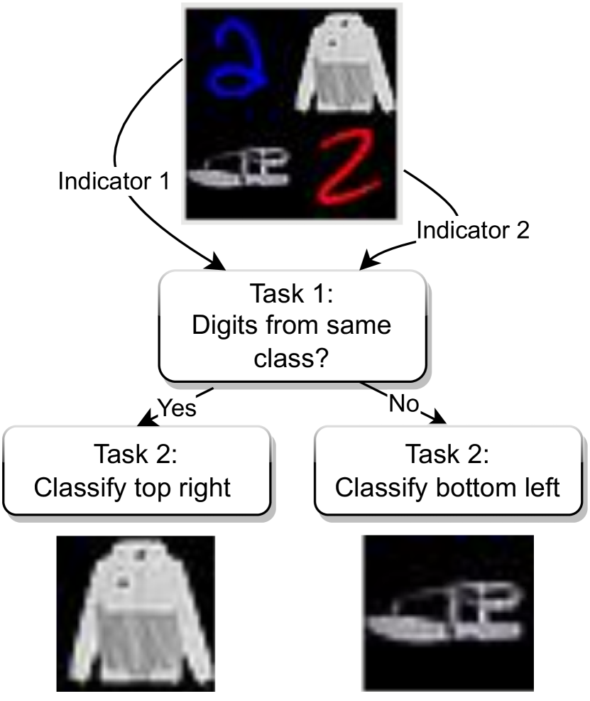
(a)

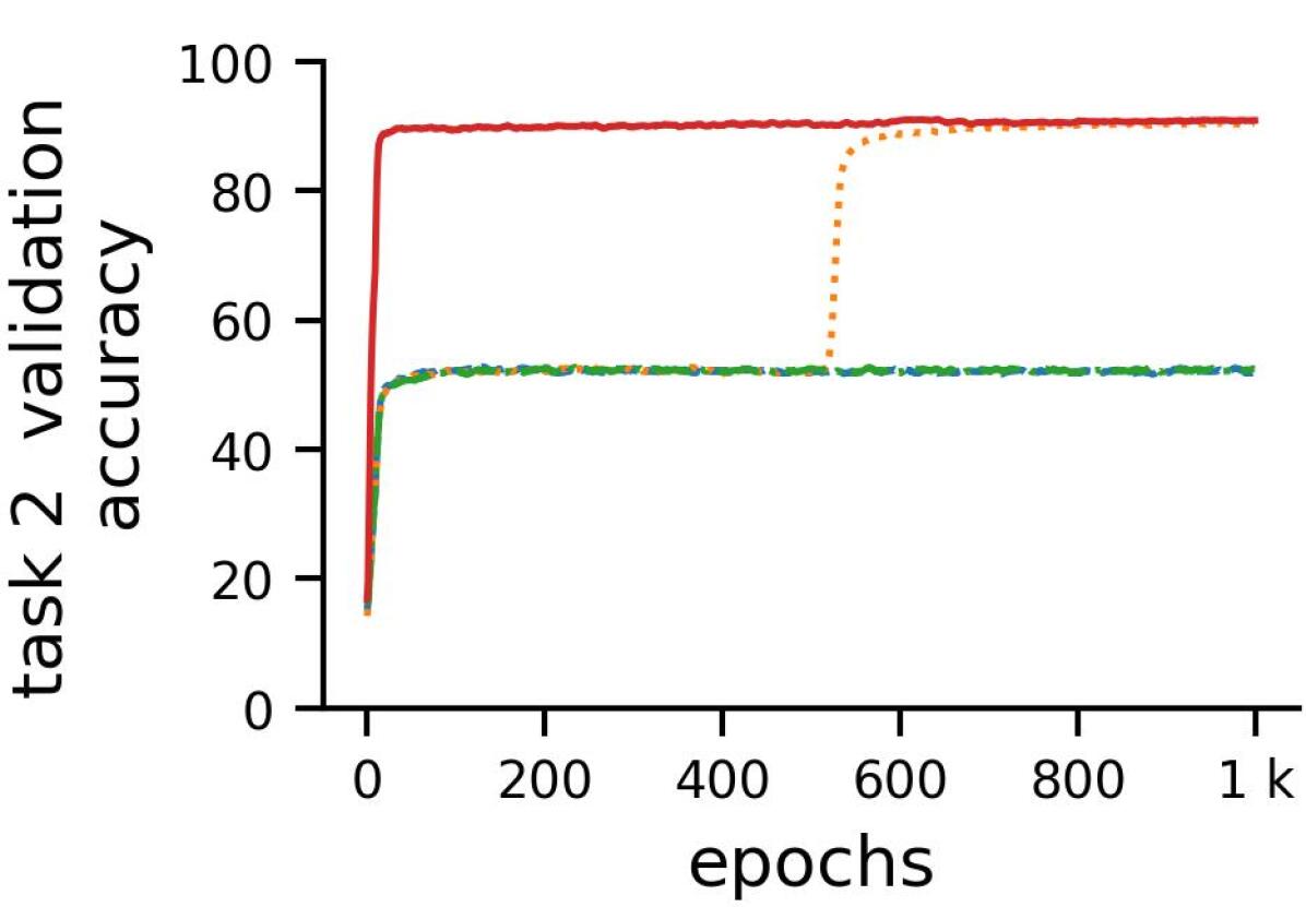
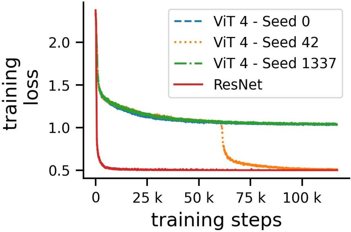
(b)

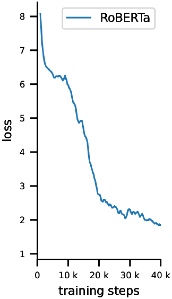
(c)

Figure 1: Transformers can get stuck during optimization for two-stage tasks. (a) Describes our 2 step decision task used to study Eureka-moments. Task 1 is to compare the two indicators (here digits). If the digits are the same, task 2 is to classify the top-right image and bottom left else. Top-right and bottom left are referred to as targets. The location of the correct target is referred to as target location. (b) Validation accuracy and training loss for the task in (a). 2 ViTs (blue and green) fail to converge, while ViT with seed 42 (yellow) has an Eureka-moment. Eureka-moments are characterised by a sudden increase of accuracy and drop of the loss. ResNets are not susceptible to this kind of optimization difficulty. (c) Eureka-moments for a real dataset. Sharp drops of the training loss after initial plateauing can also be observed for RoBERTa pretraining.

In summary, the contributions of this analysis paper are: 1) we study multi-step learning without intermediate supervision by fully controlling the data-generating process through synthetic data generation. 2) We discover a new failure mode of transformers. 3) We analyse the mechanisms underlying this failure mode and find that the Softmax function causes small gradients for the key and value weight matrics, thereby hindering learning. 4) To validate the role of Softmax, we mitigate the failure mode through small interventions. We show that these interventions lead to significantly faster convergence, higher accuracy, higher robustness towards hyper-parameters and higher probability of model convergence, affirming our analysis. Code will be made available soon.

2 Related Works

Emergence and phase transitions. Our work is weakly connected to work on emergence and phase transitions as defined by Steinhardt (2022); Wei et al. (2022). Here, emergence refers to a qualitative change in a system resulting from a quantitative increase of either model size, training data or training steps. Phase transitions describe the same phenomenon but require the change to be sharp. Eureka-moments are special types of phase transitions. Recent discoveries of phase transitions might be an artefact of the discontinuous metrics (Schaeffer et al., 2023; Srivastava et al., 2022). In our case, also smooth metrics change rapidly. A connection between phase transitions or emergence and our work may exist, and both may be related to escaping bad energy landscapes as in our work.

Unexplained phase transitions. Previous works reported observations that may be Eureka-moments, without investigating their cause. For instance, rapid improvements happen for in-context-learning (Olsson et al., 2022) and BERT training (Gupta & Berant, 2020; Deshpande & Narasimhan, 2020; Nagatsuka et al., 2021). Deshpande & Narasimhan (2020) propose to bias attention towards predefined patterns and observed speed-up in BERT training. In our work, we also identify the learning of the right attention pattern to be the problem, suggesting a common underlying phenomenon.

Grokking. A similar phenomenon has been discovered on synthetic data (Power et al., 2022) and was further studied in (Liu et al., 2022b; Nanda et al., 2023; Thilak et al., 2022; Millidge, 2022; Barak et al., 2022; Liu et al., 2022a). Grokking describes the phenomenon of sudden generalization after overfitting, which can be induced by weight decay. In contrast to Eureka-moments, the training accuracy already saturates at close to $100\text{\,}\mathrm{\%}$ (overfitting), a long time before the validation accuracy has a sudden leap from chance level to perfect generalization. For Eureka-moments, validation and training loss saturate (no overfitting) and the sudden leap occurs for both simultaneously.

Unstable gradients in transformers. The position of the layer-norm (LN) (Xiong et al., 2020) and instabilities in the Adam optimizer in combination with LN induced vanishing gradients (Huang et al., 2020). Removing the LN (Baevski & Auli, 2018; Child et al., 2019; Wang et al., 2019) or Warmup (Baevski & Auli, 2018; Child et al., 2019; Wang et al., 2019; Huang et al., 2020) resolves this problem, but in our case, Warmup alone does not help. Others identified the Softmax as one of the problems, showing that both extremes, attention entropy collapse, i.e. too centralized attention (Zhai et al., 2023; Shen et al., 2023) and a large number of small attention scores, i.e. close to maximum entropy (Dong et al., 2021; Chen et al., 2023) can lead to small gradients (Noci et al., 2022). As a remedy to vanishing gradients caused by entropy collapse Wang et al. (2021) proposed to replace the Softmax by periodic functions. However, before Eureka-moments, the attention distribution is in neither extreme. Instead the attention is allocated to the wrong tokens.

Temperature in Softmax. A key operation in the transformer is the scaled dot-product attention. Large products can lead to attention entropy collapse (Zhai et al., 2023; Shen et al., 2023), which results in very small gradients. In contrast, Chen et al. (2023) observed close to uniform attention over tokens. They scaled down very low scores further while amplifying larger scores, but this only amplified the problem when important tokens are already ignored. Instead, Jiang et al. (2022) proposed to normalize the dot product. Their proposed NormSoftmax avoids low variance attention weights and thus avoids the small gradient problem. We found it as the most effective intervention on the Softmax function. Others proposed to learn the temperature parameter (Dufter et al., 2020; Ali et al., 2021), but this is difficult to optimize. For very large models the problem becomes more severe. Models with more than 8B parameters show attention entropy collapse (Dehghani et al., 2023). They followed Gilmer et al. (2023) and normalized the $QK^{T}$ with layer norm before the Softmax.

3 Background

Preliminaries. This work investigates the dot product attention (Vaswani et al., 2017), defined as

$$\text{Attention}(Q,K,V)=\text{softmax}\left(\frac{QK^{T}}{\tau}\right)V,$$ (1)

where the weight matrices $W_{Q}$, $W_{K}$ and $W_{V}$ map the input $X$ to query $Q$, key $K$, value $V$, and the temperature parameter $\tau$ controls the entropy of the Softmax distribution. A low temperature leads to low entropy, i.e. a more “peaky” distribution. Commonly, $\tau$ is set to $\sqrt{d_{k}}$, where $d_{k}$ is the dimensionality of $Q$ and $K$. Thus, $\sqrt{d_{k}}$ is the standard deviation of $QK^{T}$ under the independence assumption of rows of $Q$ and $K$ with 0 mean and variance of 1 (Vaswani et al., 2017).

Softmax attention can cause vanishing gradients. Attention entropy collapse, i.e. too centralized attention, can cause vanishing gradients (Zhai et al., 2023; Shen et al., 2023), since all entries of the Jacobian of the Softmax will become close to 0 (see appendix). Similarly, uniform attention can result in vanishing gradients for $W_{K}$ and $W_{Q}$, as shown by Noci et al. (2022).

A remedy to both problems is to control the attention temperature $\tau$. A larger $\tau$ in the Softmax will dampen differences of $QK^{T}$ and by that prevent vanishing gradients by low attention entropy. In contrast, a smaller $\tau$ will amplify differences of $QK^{T}$ and prevents vanishing gradients caused by uniform attention. Obviously, choosing the right temperature is difficult and can have a strong influence on what the model will learn, how fast it will converge etc. One of our interventions to test whether the Softmax is indeed the root cause is Heat Treatment (HT). We suggest to start training with a low temperature and follow a schedule to heat it up to the default value of $\sqrt{d_{k}}$. This approach has multiple advantages. First, the network gets optimized for “more peaky” attention, but the temperature increases steadily. By that, the network starts with centralized attention but since the next epochs attention will be more uniform than the previous, it does not run into the issue of low attention entropy. Second, the network can focus on most important features early in training and broaden the view over time, attending to other features.

NormSoftmax. An alternative to tame the attention is NormSoftmax (Jiang et al., 2022). Here, the expected standard deviation $\sqrt{d_{k}}$ gets replaced by the empirical standard deviation $\sigma(QK^{T})$. This is done for each attention block in the transformers individually. NormSoftmax can be computed by

$$\text{NormSoftmax}(Q,K)=\text{Softmax}\left(\frac{QK^{T}}{min(\sigma(QK^{T}),\tau)}\right).$$ (2)

If $QK^{T}$ has low standard deviation differences will be amplified. If $\sigma(QK^{T})>\tau$, $\tau$ will be used.

4 Task description and experimental conditions

Task description. All our datasets follow a multi-step structure. While arbitrarily many-step tasks are possible, we only consider two-step tasks in this work, as we found it sufficient to study the phenomenon. A schematic for one of our tasks can be seen in Fig 1(a). The successive tasks in this work are referred to as task 1 and task 2. Task 1 indicates what task 2 is for a particular sample (e.g. where to look). For our vision datasets, the information provided by task 1 is which of the 2 possible targets (i.e. top or bottom) should be classified. On the vision datasets, task 2 is a simple classification task (what is the class at the indicated position?). Only task 2 is evaluated and, thus, direct supervision is only provided for task 2. By design of the datasets, $40-55\%$ accuracy can be obtained by only solving task 2 and picking the target at random. The range is due to varying difficulty of task 2. To obtain higher accuracy, both tasks must be solved.

Vision dataset creation. The visual datasets are based on MNIST (LeCun et al., 2010) and Fashion-MNIST (Xiao et al., 2017). An example and a schematic of the task is shown in Fig. 1(a). For this dataset, samples are created by sampling 2 random Fashion-MNIST samples and 2 digit samples from the MNIST classes “1” and “2”. We apply a random color to the MNIST samples (red or blue). Next, we compose a new image from the 4 images, putting the 2 MNIST samples on top left and bottom right and the Fashion-MNIST samples on the remaining free quadrants. If the 2 MNIST samples are from the same class, the class of the top-right image is the sample label and bottom-left else.

Reasoning task. To show that the problem is more general, we simplify the task to a minimum and create a reasoning task. We consider equations of the form: where $a,b,c,d\in\{0,\;1,\;...,\;n\}$ and define task 1 as follows: $g(a,\;b)=\mathbbm{1}[(\textrm{a is even}\land\textrm{b is odd})\lor(\textrm{a is odd}\land\textrm{b is even})]$. Task 2 is just classification of $c$ or $d$. More details provided in A.12.

Metrics. We define the Eureka-ratio as the proportion of training runs with Eureka-moment across the different random seeds. To automatically detect Eureka-moments, we set a conservative threshold at the validation accuracy of $70\%$, where $~{}50\%$ can be reached solving only task 2. Accuracy after Eureka-moment, in the following referred to as accuracy, is computed over all runs that had an Eureka-moment. Thus, this metric has to be considered in conjunction with the Eureka-ratio, since high accuracy with low Eureka-ratio indicates a difficult optimization or a “lucky” run. Finally, average Eureka-epoch highlights the average epoch at which the Eureka-moment happened. It is computed only for runs with Eureka-moment and should be interpreted jointly with Eureka-ratio.

Models and hyper-parameters. Following Hassani et al. (2021), we use a ViT version specifically designed for small datasets like MNIST (LeCun et al., 2010) or CIFAR (Krizhevsky et al., 2009). Unless otherwise stated, we train a ViT with 7 layers, 4 heads and set the MLP-ratio to 2, a patch size of 4 and embedding dimension of 64 per head. As a result the default temperature is $\sqrt{d_{k}}=8$. The ResNet we compared to has a comparable parameter count and consists of 9 layers. For ViT, ViT+HT and NormSoftmax we tested 5 different temperature parameters in initial experiments. More details on the architectures and training setup are provided in the appendix. For the reasoning task, we train a transformer on $30\text{\,}\mathrm{\%}$ of the entire set of possible inputs (i.e. $11^{4}=14\,641$ input combinations) for 10K epochs over five random seeds. More details on model and training are provided in the appendix.

5 Understanding Eureka-moments and the optimization challenges of transformers

Here, we analyze the problem on the dataset described in Fig. 1(a). In Sec. 5.3 we provide experiments on 2 more datasts and finally show indications, that the results can be transferred to real datasets.

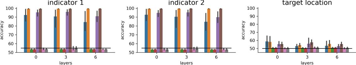
(a) ViT (fails to learn task 1)

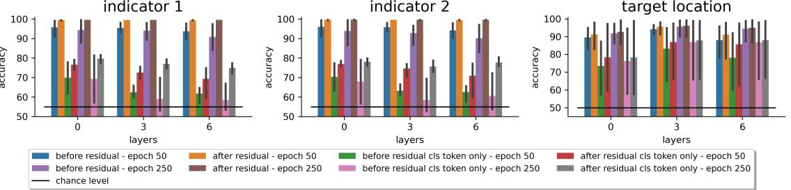
(b) ViT+HT (learns task 1)

Figure 2: Which information is represented in different parts of the network for (a) ViT (without Eureka-moment) and (b) ViT+HT (with Eureka-moment). Bar plots show linear probe accuracies averaged over heads. Indicator 1 is the top MNIST digit, indicator 2 the other. Both, ViT and ViT+HT extract the indicator class information from the images and it is available in each layer. Information is available before and after the residual connection, therefore it is not entirely ignored by the attention. Differences between ViT and ViT+HT visible for CLS token and target location task. Error bars show variance over heads. More layers, representations and targets are shown in appendix.

5.1 Why do transformers fail to learn simple two-step tasks?

To investigate why ViT’s learning fails, we analyze the learned representations. Note that solving task 1 requires ViT to 1) learn to distinguish the indicators, 2) carry the information through the layers and 3) compare the indicator information to obtain the target location. We investigate these questions in the following by learning linear probes on the output of the attention heads, i.e. $Z_{i}=\text{Attention}(Q_{i},K_{i},V_{i})$, for all heads $i$. However, note that linear separation becomes very likely as the dimensionality of the features increase. Therefore, a high accuracy on the linear probe classification does not imply that the transformer is capable of using the information, only that it is represented and linearly separable. While the linear probe training has supervision on task 1, the transformer does not.

Does the transformer fail to distinguish the indicators? The two left bar plots in Fig. 2(a) show that the indicators can be almost perfectly separated by linear probes in all layers. Still ViT fails to learn task 1 (orange, brown). Interestingly, the indicators are already separable in early stages of the training (orange). Consequently, the transformer represents the necessary features to possibly distinguish the indicators.

Does the transformer filter out information required for task 1? Since the loss provides a training signal only for task 2, the transformer may learn to just ignore the indicators. The residual connection in the transformer block makes ignorance of features unlikely but not impossible. Task 1 information could be ignored in the attention blocks s.t. it cannot attend to compare the indicator classes. To test this, we probe the representation after the attention operation before and after the residual connection. Fig. 2(a) reveals that the indicator information is available in all layers. Early in training, some indicator information is filtered out in the attention block (blue). Indicator information is partially filtered out in deeper layers, but is always recovered by the residual connections. We show the linear probe results based on the output of the Softmax $Z_{i}$. Plots for $Q_{i}$ and $K_{i}$ look similar. Therefore, it is evident that the features to solve task 1 are not filtered out.

ViT

$\text{ViT }\tau$=1/3

ViT+HT

NormSoftmax

Figure 3: Gradients on image for $W_{k}$ at Epoch 50. For ViT the gradient for $W_{K}$ comes mostly from target regions, while for the other approaches indicator regions provide substantial gradient. Detailed explanation of this plot and plots for $Q$ and $V$ can be found in Sec. A.2

Does the transformer fail to combine the information? We observe that the target location ( solution of task 1) cannot be inferred by the linear probe with high accuracy (Fig. 2(a)). This implies that even though the (indicator) information is present within the feature representations, it does not allow easy combination to predict the target location needed for task 2. In conclusion, the transformer has all the necessary information, but fails to combine it to solve the multi-step task.

Differences to a transformer that had an Eureka-moment. Fig. 2(b) shows the linear probe results for a transformer that learns task 1. Interestingly, the target location can be predicted by linear probes from all layers and all tested representations with high accuracy. This is in stark contrast to transformers that had no Eureka-moment. The second striking difference is that indicator information is represented in the CLS token. This is even stronger for early layers. We suspect that the information is written to the CLS token to solve the indicator class matching.

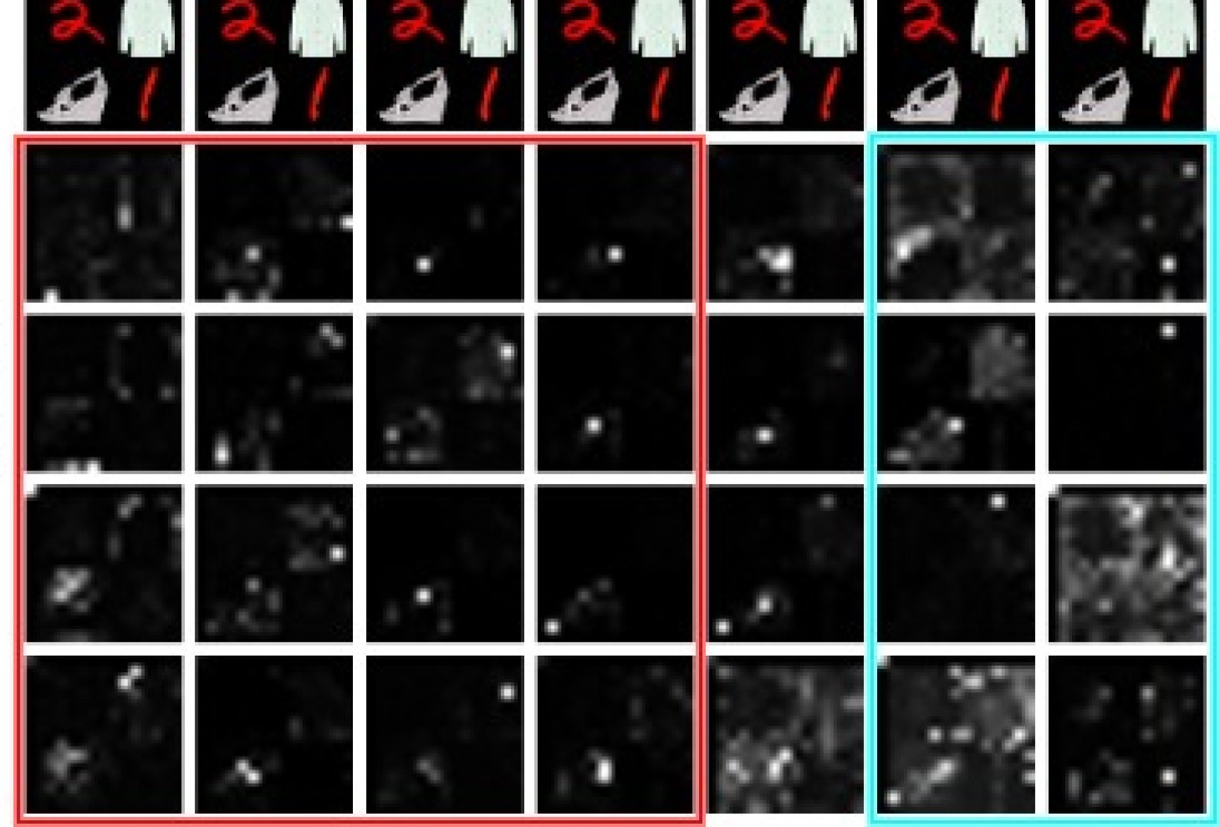
(a) ViT without Eureka-moment

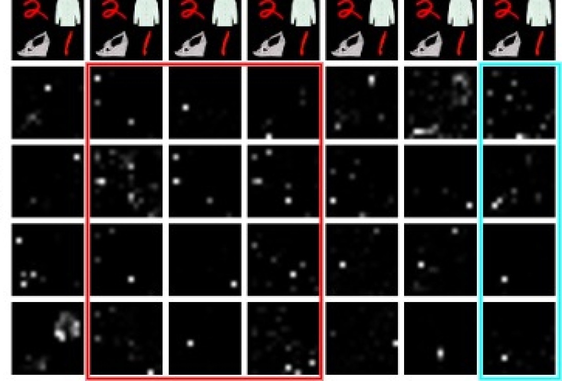
(b) ViT+HT with Eureka-moment

Figure 4: Attention maps after training for: (a) ViT without Eureka-moment, i.e. fails to compare the 2 digits. First layers explicitly ignore indicators (digits) (highlighted with red). (b) ViT+HT with Eureka-moment attends indicators in first layers (red) and predominantly attends the correct target (ankle boot) in later layers. Black is no attention and white is high attention. Maps show the average attention of each query $q$, i.e. we average over the key-dimension of the attention map.

How does the transformer fail to combine the information? To obtain a comprehensive understanding of the reasons of the failure to combine information, we visualize the attention maps of two fully trained ViTs in Fig. 4. We find that the transformer without Eureka-moment does not attend the indicator digits and attends only the targets of task 2, whereas a transformer with Eureka-moment attends the indicator digits in early layers. This suggest that a ViT without Eureka-moment does not attend indicators enough to match them and has difficulties to learn to attend different regions.

Why does the transformer fail to learn to attend to the indicators? Based on the discussion in Sec. 3, we suspect that ill-distributed attention scores lead to small gradients for $W_{K}$ and $W_{Q}$, which in turn inhibit learning. Note that high attention to some pairs with low attention to all others or uniformly distributed attention can result in vanishing gradients (Noci et al., 2022). To test this, we visualize the L1-norm of the gradient for the first layer in Fig. 5. For vanilla ViT that gradients for $W_{K}$ and $W_{Q}$ are 0.5-1 orders of magnitude smaller than those for $W_{V}$. Thus, small gradients are passing the Softmax, reaching $W_{Q}$ and $W_{K}$ and the attention map improves only slowly, which results in the observed learning difficulties. Differences between the gradients are much smaller for ViT $\tau=\frac{1}{3}$, ViT+HT and NormSoftmax, in particular before the Eureka-moment. Fig. 3 shows the origin of gradients on the image plane for $W_{k}$. For ViT, the gradients mostly originate from the target regions, which further explains why many steps are needed to move attention to the indicators.

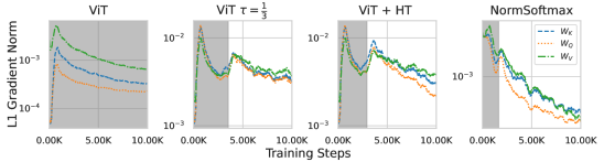
Figure 5: L1 gradient norm during training for $W_{K}$, $W_{Q}$ and $W_{V}$ for the first layer. For ViT, $W_{K}$ and $W_{Q}$ receive much smaller gradients than $W_{V}$. In particular before Eureka-moment (gray regions), the differences between gradient magnitudes are much smaller for smaller temperatures or NormSoftmax. The y-axis is log scaled. All layers shown in Fig. 12.

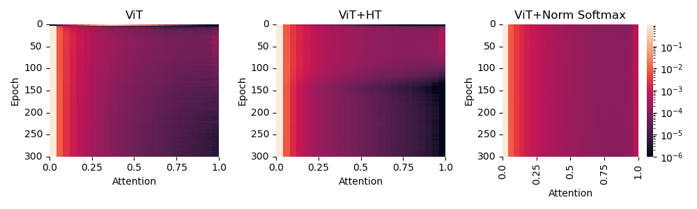
Figure 8: Attention distribution as a heatmap. Attention scores are sampled during evaluation after each epoch and binned to 25 bins. The color map is log scaled. For all 3 models, the vast majority of values falls into the first bin. ViT shows very few higher attention scores. ViT+HT and ViT+NormSoftmax lead to a significantly larger number of medium and high attention values. For ViT+HT this is limited to the first 100 epochs.

Is too small or too large attention-entropy the problem? As discussed, low or high attention entropy can both result in vanishing gradients. We visualize the distribution of attention maps over training in Fig. 8. It is apparent that the vast majority of attention scores is very small, indicating that a too uniform attention is causing small gradients. Larger attentions are rare, but not absent, as can be seen in Fig. 4(a), but indicator regions have small and uniform attention. Thus, we conclude that local uniform attention causes the transformer’s learning problems.

5.2 Can enforcing lower entropy attention maps resolve the small gradients?

In the previous subsection, we concluded that local uniform attention is causing learning problems. To demonstrate this, we aim to modify the attention to remedy this issue. Particularly, we modify Softmax’s temperature $\tau$ in the attention block. Large temperatures increase entropy, while small temperatures decrease it. We test various settings, training simply with lower temperature, HT, where the temperature increases from a low value to default temperature during the first half of the training and NormSoftmax, which adaptively changes the temperature for each sample, head and layer.

Does a lower temperature solve the small gradient issue and thereby mitigate the optimization issues? Increasing the temperature from low to default or using NormSoftmax increases high attention scores (c.f. Fig. 8). More importantly, the transformer learns to also attend to the indicators (Fig. 4(b)). As a result, all approaches (lower temperature $\tau$, HT and NormSoftmax) solve the imbalanced gradient issue for $W_{V}$, $W_{Q}$ and $W_{K}$ (Fig 5) and lead to higher gradients in indicator regions (Fig. 3).

As a result, the interventions indeed mitigate the optimization issues. Eureka-moments happen much earlier or instantly (see Fig. 7(a)). A comprehensive comparison between a vanilla ViT and other versions is provided in Tab. 1. Decreasing the temperature and using NormSoftmax increases the Eureka-ratio, accuracy and decreases the Eureka-epoch (i.e. improving the energy landscape). In contrast, increasing the temperature has a negative effect on the Eureka-ratio, supporting that the local uniform attention is the main cause for the learning problem.

5.3 Is this an artificial problem caused by other factors?

Table 1: Comparison of proposed solutions and baselines. For the main dataset, as described in Fig. 1(a). and the No position task (Fig. 7(b)). $\tau$ not optimized for No position task. ER: Eureka-ratio, Acc.: Accuracy, Avg. EE.: average Eureka-epoch.

		Main Dataset			No Position Task
			Avg. over EMs		Avg. over EMs
Model	$\tau$	ER $\uparrow$	Acc. $\uparrow$	Avg. EE.	ER $\uparrow$	Acc. $\uparrow$	Avg. EE.
ViT	$\frac{1}{0.025}$	3/10	89.40	174.67	-	-	-
ViT	$\frac{1}{0.075}$	6/10	90.13	181.34	-	-	-
ViT + WD 0.5	$\sqrt{d_{k}}$	5/10	90.09	177.8	-	-	-
ViT	$\sqrt{d_{k}}$	7/10	89.48	207.43	0/4	-	-
ViT + Warmup 20	$\sqrt{d_{k}}$	8/10	87.65	205.87	1/4	89.55	117
$W_{QKV}$ grad scaling	$\sqrt{d_{k}}$	10/10	87.96	119.4	0/4	-	-
NormSoftmax	$\sqrt{d_{k}}$	10/10	89.56	28.2	3/4	88.98	228
NormSoftmax	$\frac{1}{3}$	10/10	89.18	23.5	1/4	89.77	20
ViT	$\frac{1}{3}$	10/10	89.35	66.6	1/4	89.68	191
ViT+HT	$\frac{1}{3}\rightarrow\sqrt{d_{k}}$	10/10	89.81	74.0	1/4	88.36	242
NormSoftmax + HT	$\frac{1}{3}\rightarrow\sqrt{d_{k}}$	10/10	89.83	17.5	1/4	90.63	19

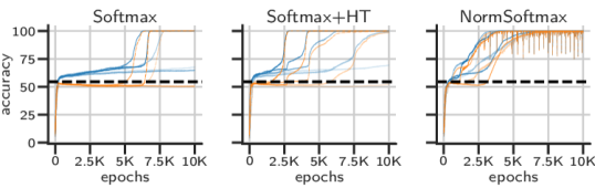
(a)

Figure 6: (a) Eureka-moments for single-layer transformers on a simple reasoning task. We show the train (blue) and test (orange) accuracies for attention with Softmax, Softmax+HT, or NormSoftmax, over 5 random seeds (transparencies). Chance probability is $6/11\approx$54\text{\,}\mathrm{\%}$$ (black). (b) Eureka-moments in real dataset. Sharp drops after initial plateauing can be observed also for RoBERTa pretraining. Using NormSoftmax leads to an earlier Eureka-moment.

 

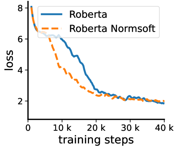
(b)

Does the transformer simply ignore specific indicator locations? The task and dataset used in the previous subsections showed indicators and targets always at the same location, i.e. indicators on top-left and bottom right. Such a dataset design might result in two undesired effects: 1) The transformer might learn to ignore features based on the associated positional embeddings. 2) The task might be easier, since positional embeddings can be used as shortcut to find indicators without the need to rely on the actual features. To test for both cases we create another dataset. Refer to Fig. 7(b) for the dataset and task description. We observe that removing the fixed position for indicators and targets makes the task even more difficult (Tab. 1 right) and differences between methods are even more apparent. Thus, ViTs without Eureka-moment do not simply learn to ignore regions of the image. More datasets are described in A.9.

Is this a vision or feature extraction problem? To show that Eureka-moments transcend mere artifacts of vision data, we also show their occurrence in the context of simplistic algorithmic tasks, referred to as the reasoning task. Due to the simplicity of the task, we use a single-layer 4 head transformer model. Fig. 6(a) reveals that Eureka-moments appear even in this simplified task, which does not require any feature learning. Both HT and NormSoftmax reduce the training steps required for Eureka-moments to occur and increase the Eureka-ratio from 3/5 to 4/5 or 5/5, respectively.

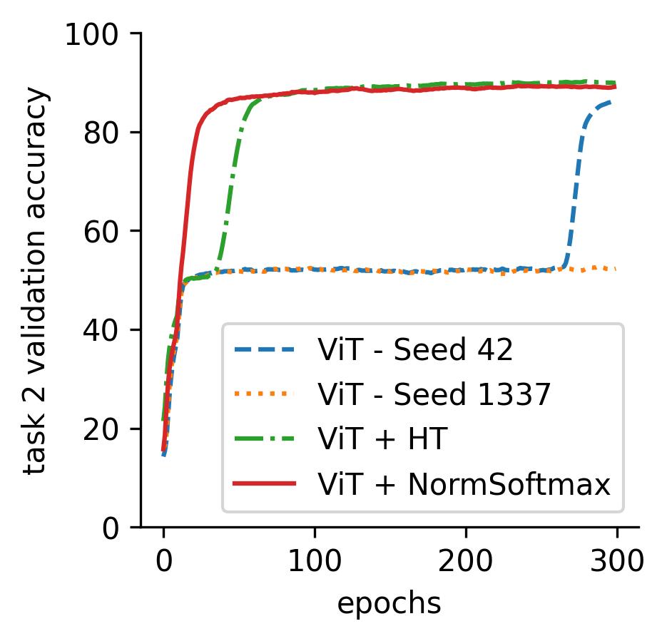
(a)

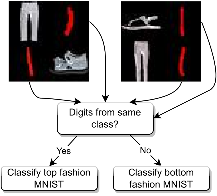
(b)

Figure 7: (a) Validation accuracy curves on main dataset. (b) No position task description. This task removes more information by shuffling the rows of each data sample, i.e. classify either the top or bottom fashion sample. Two samples are shown to highlight differences from the task described in Fig. 1(a).

 

Is this a mere artefact of a bad choice of hyper-parameters? We always use the default of 5 Warmup epochs to avoid training instabilities during early stages of training. We found that 20 Warmup epochs were most effective in mitigating the problem. However, sensitivity to the learning rate schedule (Tab. 2) is high. The average Eureka-epoch is very late (Tab. 1 left) and we found more Warmup epochs lead to worse results on harder tasks (Tab. 1 right). We also find that the Eureka-ratio is sensitive to the learning rate schedule. We test 9 learning rate schedules for each method, (see Tab. 11). Lower temperatures are less sensitive to the learning rate schedule (see Tab. 2).

Table 2: Sensitivity to learning rate schedule. Lower temperatures and in particular NormSoftmax drastically increase robustness to imperfect learning rate schedules. Eureka-ratio computed over seeds and learning rate schedules.

Model	Eureka-ratio $\uparrow$
ViT	04/36
VIT + Warmup 20	14/36
$W_{QKV}$ grad scaling	5/36
NormSoftmax	36/36
ViT $\tau=\frac{1}{3}$	20/36
ViT+HT $\frac{1}{3}\rightarrow\sqrt{d_{k}}$	25/36

Weight Decay (WD) can facilitate grokking (Power et al., 2022) by forcing the network to learn general mechanisms (Power et al., 2022; Nanda et al., 2023). In our setting, we only found mild improvements for higher WD. However, more random seeds revealed, that higher WD rather reduces the Eureka-ratio (Tab. 1) and does not help in solving transformer’s learning issue.

Influence of model scale on Eureka-ratio. We found no consistent influence of model scale on Eureka-ratio. More details are provided in A.5.

Can the problem be fixed by rescaling of the gradient magnitude for $W_{V}$, $W_{Q}$ and $W_{K}$? The observation that lower gradient imbalance leads to higher Eureka-ratio suggests, that simply rescaling of the gradients may solve the problem. We find that this also does not work consistently (see Tab. 1) and is very sensitive to the learning rate (see Tab. 2). We attribute this to the differences in gradient magnitudes for indicators and targets and discuss it further in Sec.A.4.

Do gradients vanish completely and can transformers recover? Fig. 1(b) already suggests, that one potential solution to reliably get Eureka-moments is very long training. This observation is supported by Fig. 5, which indicates that gradients become small, but not 0. Indeed we observe that training for 3000 epochs results in an Eureka-ratio of 4/4 for all the learning rate schedules. In practice, this is of little help because the number of sub-tasks is unknown and Eureka-moments hard to predict.

Does the NormSoftmax intervention also help on real datasets? Jiang et al. (2022) reported improved performance and faster convergence on ImageNet and machine translation tasks using NormSoftmax. Both tasks likely contain some innate multi-step tasks, e.g. identifying a common discriminative feature and then discriminating between the difficult classes for ImageNet. Improvements may be due to easier multi-step learning with NormSoftmax. Deshpande & Narasimhan (2020) showed that attention learning slows down task 2 learning for RoBERTa. Indeed, training RoBERTa (Liu et al., 2019) with NormSoftmax leads to earlier Eureka-moments (see Fig 6(b), more details in A.14). Thus, our analysis and results appear to be transferable to real datasets.

6 Limitations and Conclusion

Limitations. The ability to decompose tasks into sub-problems and learn to solve those sub-tasks is a common problem, but it is difficult to study on real datasets, since there are many confounders. As a result many works follow a trial and error approach. In contrast, we try to derive deeper understanding by studying this problem in isolation on synthetic data. This comes with the (implicit) assumption that our analysis transfers to real data, but we can provide only indications for that. We believe that both approaches provide different information that can be put together to make progress.

Conclusion. In this work, we identified that transformers have difficulties to decompose a task into sub-problems and learn to solve the intermediate sub-tasks. We observe that transformers can learn these tasks suddenly and unexpectedly but usually take a long time to do so. We call these Eureka-moments. We pin down the problem to the Softmax in the attention that leads to small gradients. We propose simple solutions that specifically target the Softmax and show that they improve the transformers’ capabilities to learn sub-tasks and to learn them faster. We identify NormSoftmax as most robust and convenient method, leading to consistently better results.

7 Acknowledgements

We thank Philipp Schröppel and the entire Computer Vision Group Freiburg for inspiring discussions. Sudhanshu Mittal for feedback on the manuscript and Matteo Farina for reporting observations of potential Eureka-moments on vision and language tasks.

Appendix A Appendix

Here, we provide additional information that supports understanding and helps interpreting the main paper. We provide supplemental experimental results and more detailed analysis. We show the gradient norm for indicators and targets individually, which reveals that most of the already small gradients for $W_{Q}$ and $W_{K}$ is attributed to target features for models that do not learn the task and very little to indicator features. We provide the linear probe plots using also $Q$, $K$ and $V$ representations and the full version of Fig. 5. Next, we provide an ablation on model scale and the main results from the main paper with standard deviation and training speed up. We explain additional datasets and report results on them. Last, we provide details on training and experimental setups and an explanation for vanishing gradients in case of centralized attention maps.

A.1 Attention distribution over time.

A.2 Gradient norm for indicators and targets.

Our particular dataset design allows us to look at the gradients for indicators and targets separately. In particular, we make use of the fact, that indicators and targets are always at the exact same spacial location. More precisely, we use the partial derivatives as proxy for the gradients. We compute $\frac{\partial Z}{\partial Q}$, $\frac{\partial Z}{\partial K}$ and $\frac{\partial Z}{\partial V}$, where $Z$ is the output of the attention function. To analyze the gradient norm for targets and indicators independently we compute $\frac{\partial Z}{\partial Q}$, $\frac{\partial Z}{\partial K}$ and $\frac{\partial Z}{\partial V}$, where $Z$ is the output of the attention function. Since we compute the derivative wrt. the tokens, the spacial dimension remains. By averaging over the batch dimension and heads we can plot the partial derivative for each token. While it’s not exactly the same, we will use the term gradient to refer to these partial derivatives in the following.

Since each token corresponds to a region in the image, we can visualize these results as an image. The results are shown in Fig. 3, Fig. 9 and Fig. 10. It can clearly be seen, that target regions (top-right and bottom-left) receive more gradients than indicator regions for $K$ and $V$. ViT, ViT+HT and NormSoftmax mitigate this problem, leading to significant gradient for indicator tokens. Indicator regions for $Q$ receive comparatively larger gradients, however, the gradients for $Q$ are much smaller.

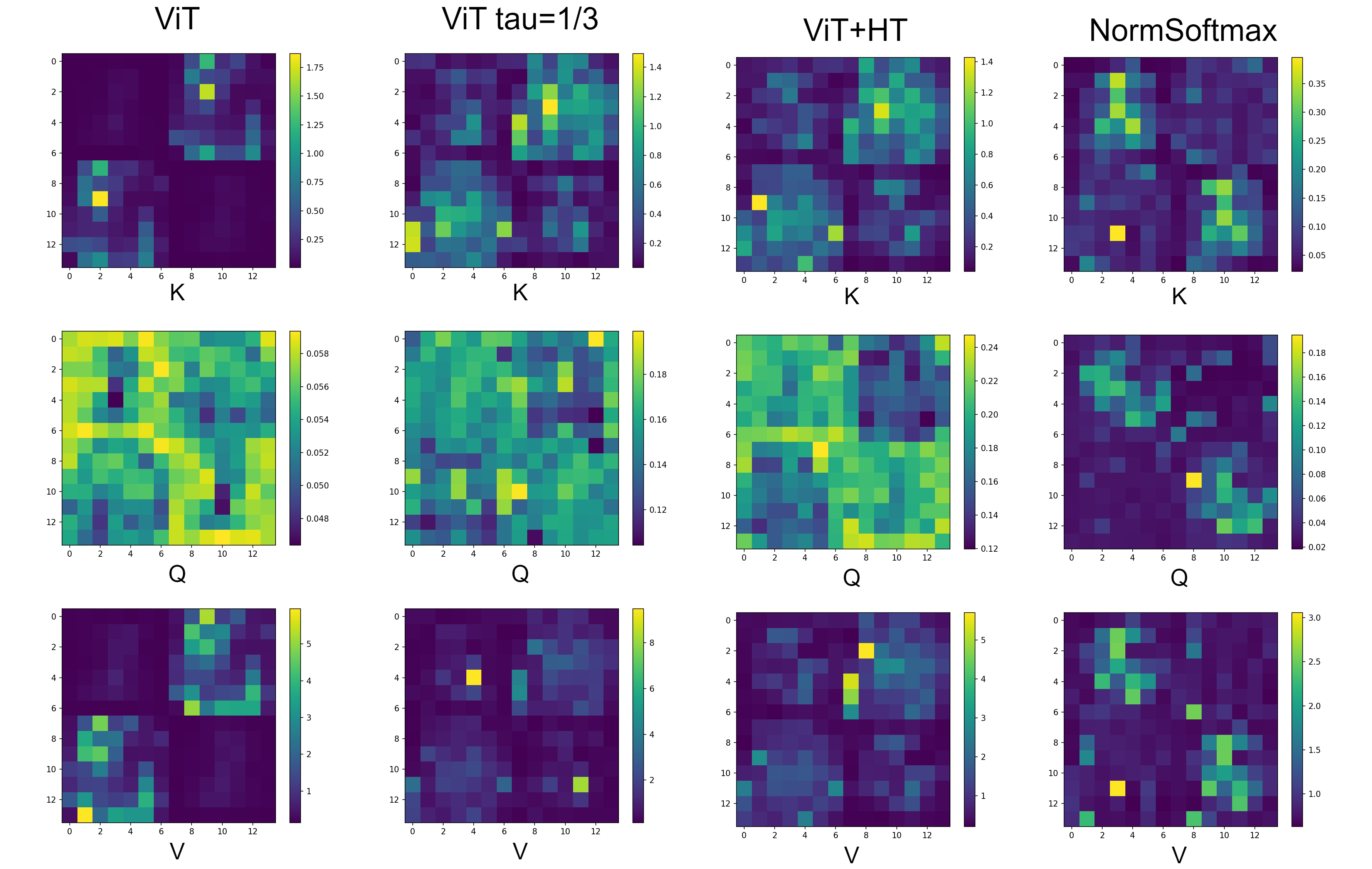
Figure 9: Gradient norm for different image regions visualized for $Q$, $K$, $V$. Larger gradients are visible for target regions, i.e, top-right and bottom-left. Indicator receive less gradients for $K$ and $V$. ViT $\tau=\frac{1}{3}$, ViT+HT and NormSoftmax mitigate this problem well. Indicator regions for $Q$ receive more gradient relative to the target regions, but overall the gradient for $Q$ is very small (see color bar). Plots created at epoch 50.

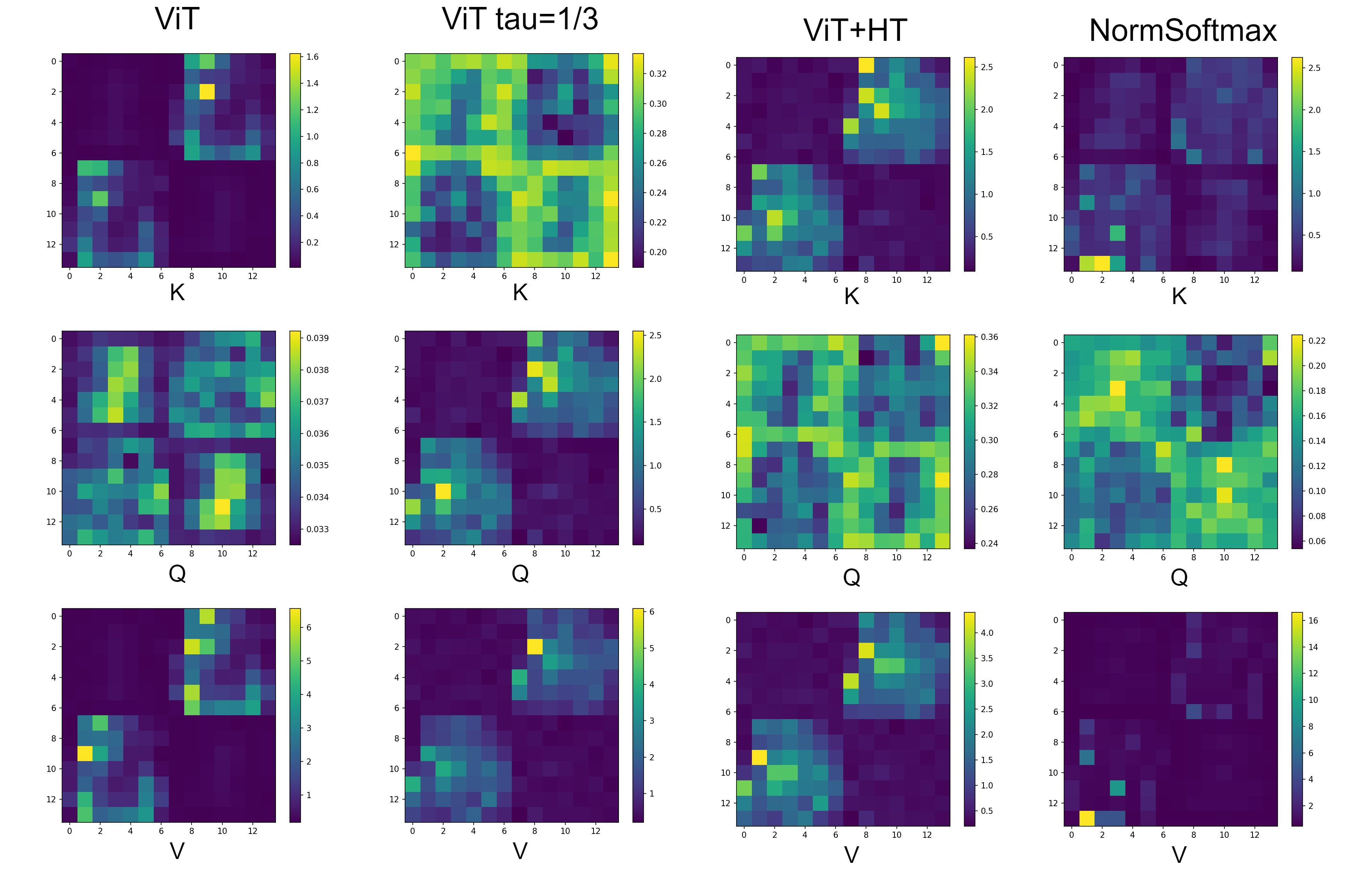
Figure 10: Gradient norm for different image regions visualized for $Q$, $K$, $V$. at epoch 13 (Eureka-moment of NormSoftmax).

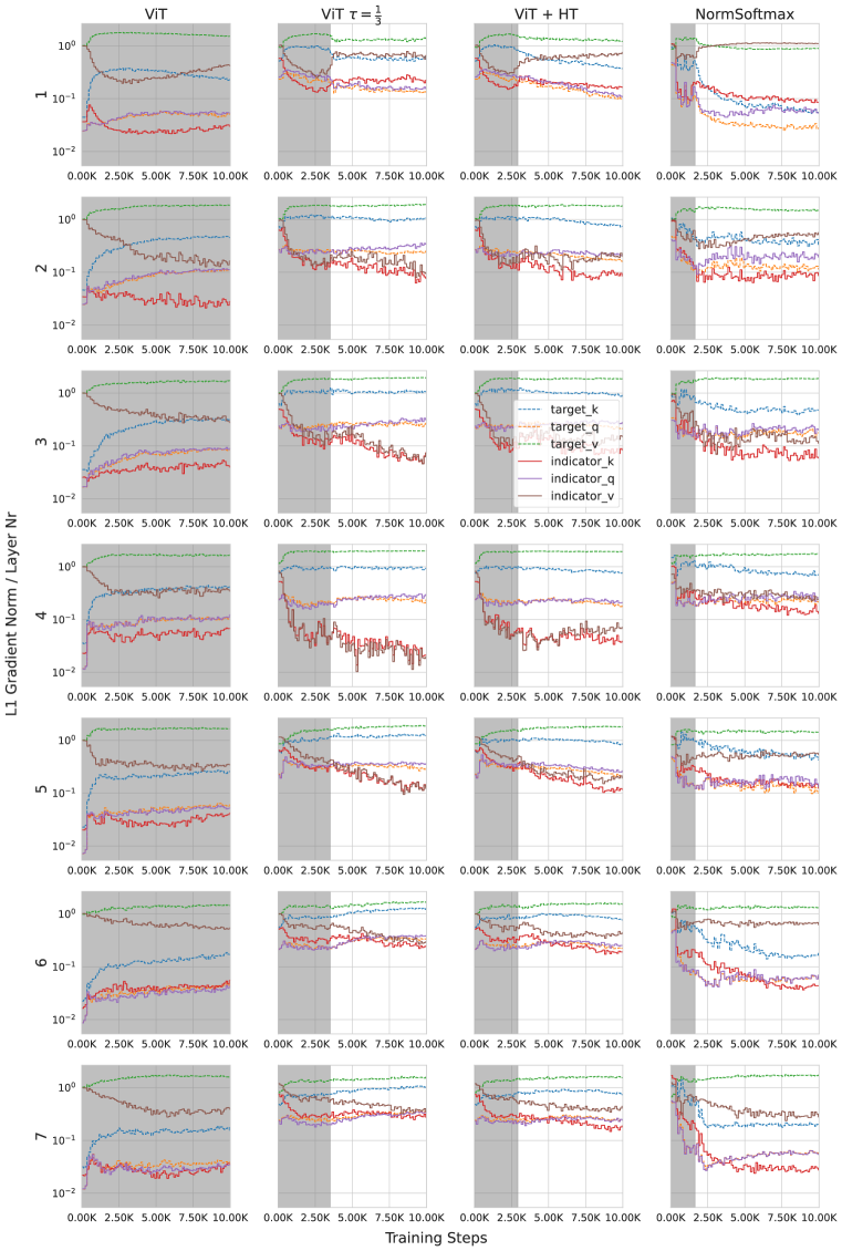
Figure 11: L1 gradient norm separately for indicator and target tokens. Indicator regions/features receive much less gradient than target regions. Gray region indicates steps before Eureka-moment.

Besides that, we compute the mean partial derivative for indicator and target regions of the image i.e. we average the partial derivatives for tokens corresponding to target regions or indicator regions. This allows us to plot the gradient norm for $Q$, $K$ and $V$ for only target and indicator tokens over the training. We show the results in Fig. 11. We make the following observations:

1. In general, the gradients are not evenly divided between target and indicator $K$, with usually smaller gradient for the indicator regions. Therefore Fig. 5 even underestimates the difference for the indicator regions, i.e. the regions relevant for an Eureka-moment.

2. This difference can explain why more time is needed to reach an Eureka-moment for ViT in comparison to the other methods.

3. This difference between indicator $k$ and target $k$ can also explain, why the $W_{QKV}$ grad scaling does not solve the problem.

4. For ViT the difference between gradients of “$V$ and $K$” and “$V$ and $Q$” is, for most layers, generally much larger compared to the other approaches. This is particularly true before the Eureka-moment, where larger gradients for indicator $K$ and indicator $Q$ are crucial to get an early Eureka-moment. Most prominent is the difference between target $V$ and indicator $K$, showing a large mismatch. This explains, why the attention maps change so slowly and why simply increasing the learning rate does not solve the problem.

A.3 Gradient Norm

Fig. 12 shows the L1 gradient norm for all layers and all methods. It can be seen, that throughout all layers and the entire training ViT has larger gradients for $W_{V}$ in comparison to $W_{K}$ and $W_{Q}$. For the other methods differences are much smaller and less consistent.

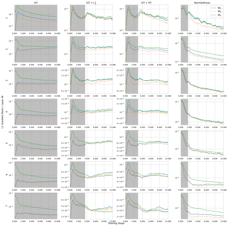
Figure 12: L1 gradient norm plot for all layers, all models and entire training. This is the complete version of Fig. 5. For ViT it can be seen that for all layers the gradient for $W_{V}$ is significantly larger than for $W_{Q}$ and $W_{K}$. For ViT+HT, ViT with $\tau=\frac{1}{3}$ and NormSoftmax the gradient norm is very similar for the weight matrices (note that the y-axis is not shared). NormSoftmax achives this also for deeper layers. Often after Eureka-moment $W_{V}$ starts to get larger attention than $W_{K}$ and $W_{Q}$. We conjecture that this is because the attention is already optimized, while task 2 can still improve by modifying the feature representation. Gray region indicates steps before Eureka-moment.

A.4 Why gradient magnitude scaling does not work.

Following the observation of Fig. 5, it stands to reason to simply scale the gradients for $W_{V}$, $W_{Q}$ and $W_{K}$ to the same value. To this end, we compute the gradient norm for $W_{V}$, $W_{Q}$ and $W_{K}$ for each layer and the overall mean. We scale the gradients for $W_{V}$, $W_{Q}$ and $W_{K}$, such that their norm is equal to the mean norm. This removes the imbalanced gradient issue and results in identical effective learning rate.

While this approach might work, it solves only part of the problem. Different features might receive differently large gradients. For instance the indicator features (here digits) receive little gradient, while target (here fashion) receive large gradients, as can be seen in Fig. 9. Simply scaling up the gradients would not solve the imbalance between indicator and target gradients.

We can see in Tab. 1, that $W_{QKV}$ grad scaling helps on the main dataset, but is very sensitive to the learning rate (Tab.2). However, it completely fails on the harder task. The learning rate sensitivity and the failure on the harder task are most likely due to the gradient imbalanced discussed above.

A.5 Influence of model scale on Eureka-ratio.

The low Eureka-ratio could also be due to a too large or too small architecture. Also the number of heads might play an important role, since different features can be attended in different heads. More heads might increase the likelihood of one head specializing in indicators. Also the embedding dimension per head might just be too small or large for the task at hand. Maybe, even the hidden dimension of the MLP at the end of the attention block is the bottleneck. Many parameters of the transformer itself could explain why it fails to solve our tasks. We test these hypotheses in Tab. 3. While most changes lead to a lower Eureka-ratio, reducing the depth and increasing the number of heads leads to mild improvements. Combining both leads to an Eureka-ratio of 4/4, but, as can be seen in Tab. 5, this architecture does not generalize to other datasets.

Table 3: Influence of model scale on Eureka-ratio. Eureka-ratio is only partially influenced by the architecture. More shallow models and more heads both improve the results. The combination leads to 4/4 Eureka-ratio, but as can be seen in Tab. 5 this architecture fails at other tasks, while our solutions lead to improvements even on the “no position task”.

					Avg. over subset with Eureka-moment
Heads	Emb. Dim.	Depth	MLP	Eureka-ratio $\uparrow$	Accuracy $\uparrow$	Avg. Eureka-epoch
4	64	7	2	2/4	88.61 $\pm$ 1.64	232.50 $\pm$ 35.50
4	64	7	4	1/4	90.16 $\pm$ 0.00	162.00 $\pm$ 0.00
4	64	4	2	3/4	88.77 $\pm$ 1.20	216.33 $\pm$ 46.64
4	64	10	2	2/4	89.93 $\pm$ 0.26	221.00 $\pm$ 18.00
4	48	7	2	1/4	90.18 $\pm$ 0.00	137.00 $\pm$ 0.00
4	96	7	2	2/4	89.76 $\pm$ 0.03	140.50 $\pm$ 70.5
2	64	7	2	0/4	-	-
6	64	7	2	3/4	89.67 $\pm$0.25	139.67 $\pm$ 55.16
6	64	4	2	4/4	89.75 $\pm$ 0.24	152.25 $\pm$ 44.49

A.6 Linear Probe results for $Q$, $K$ and $V$ and for target classification.

In the following we will show the linear probe results for $Q$, $K$, $V$ and $Z$ for all layers.

Linear probe results for $Z$ for all layers. Fig. 13 shows the same plot as in the main paper, but for all layers. In addition to the observations made for the main paper, we can see that layer 2, 3 and 6 for the ViT with Eureka-moment (Fig. 13(b)) represent significantly more information about the target locations than other layers in the CLS token. Indicating, that this information is extracted in these layers and written on the CLS token.

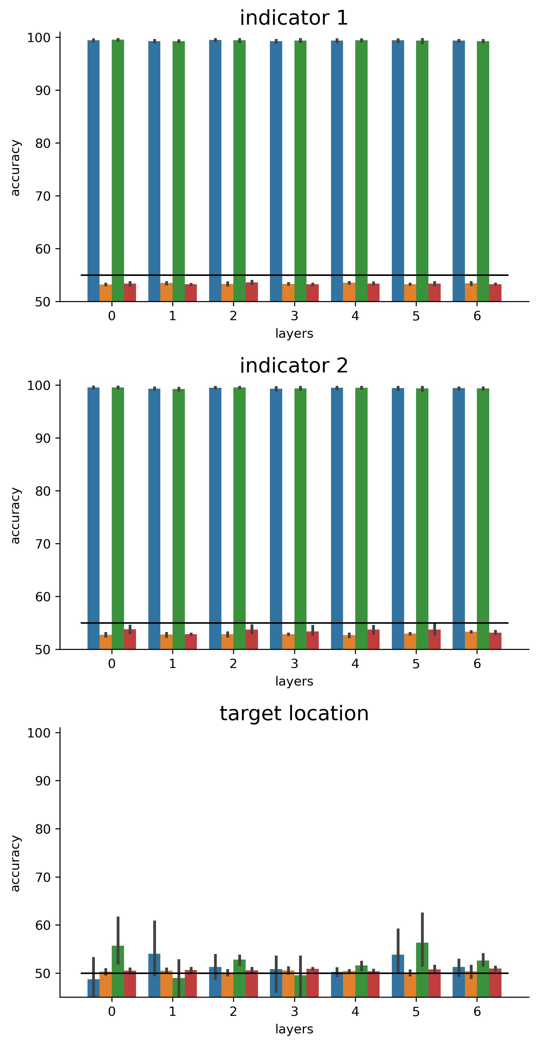
(a) ViT without Eureka-moment

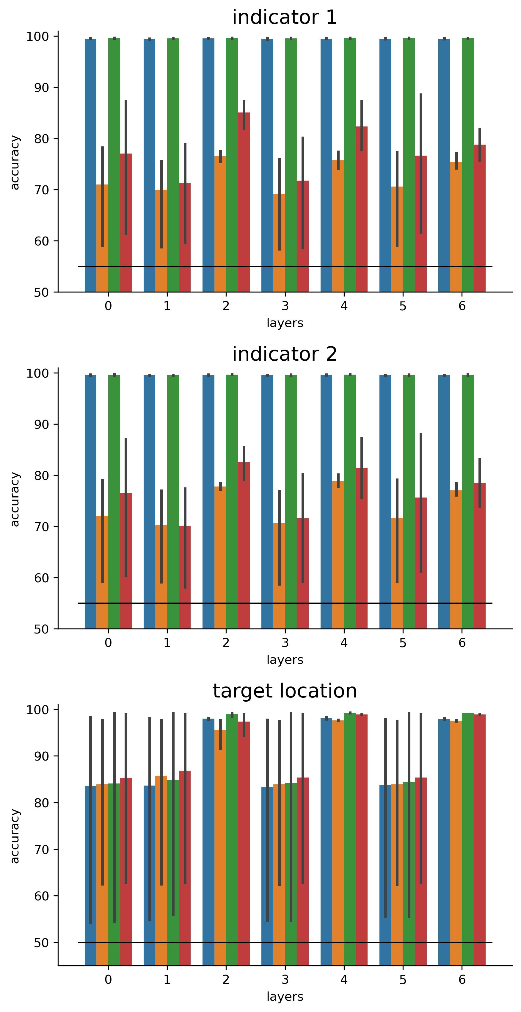
(b) ViT with Eureka-moment

Figure 16: Linear probe for Q.

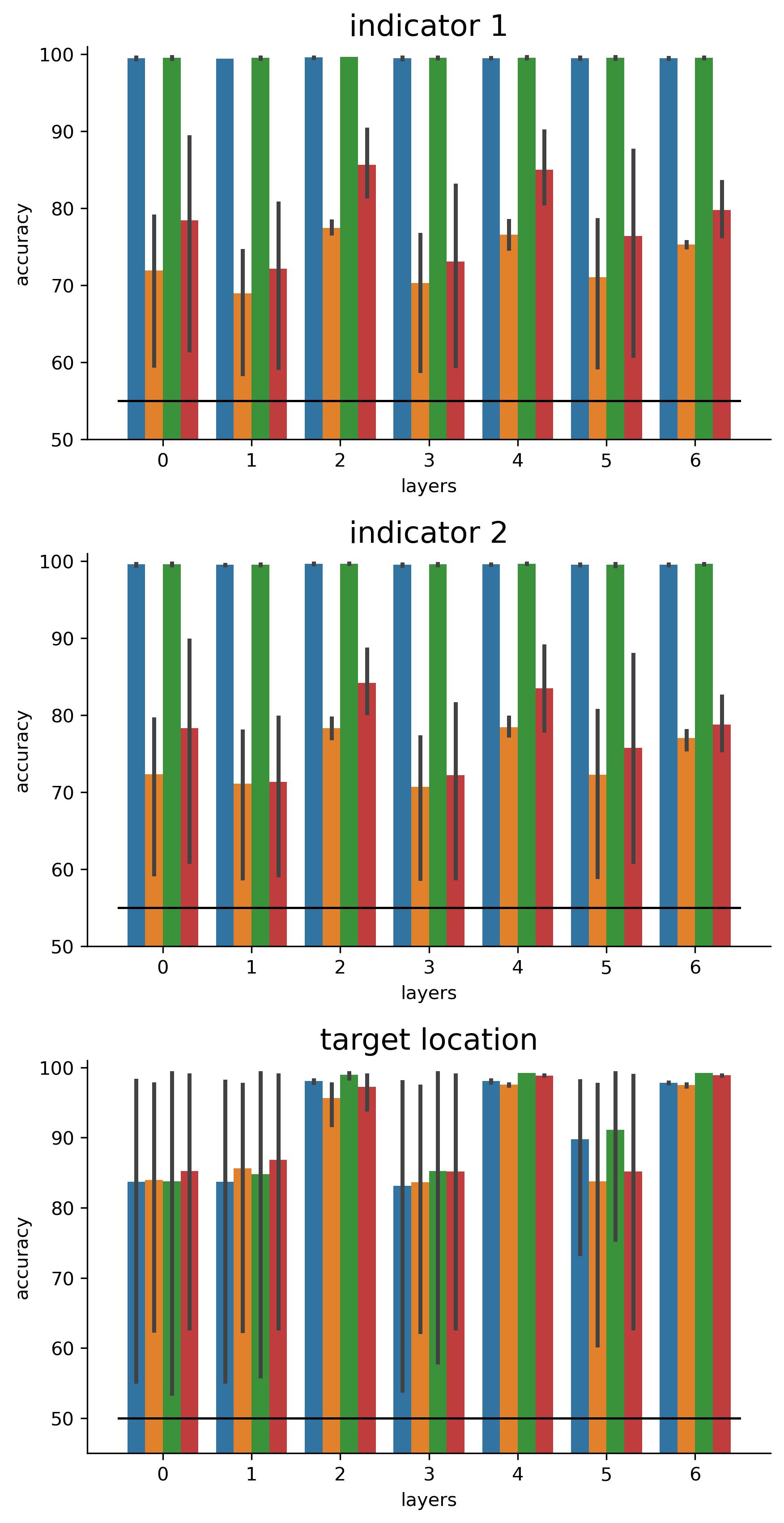
(b) ViT with Eureka-moment

Figure 17: Linear probe for K.

Linear probes for $Q$ and $K$ and $V$. Fig. 16 and Fig. 17 show the results when using the $Q$ and $K$ as input for the linear probes. Note, that $Q$ and $K$ are not updated by the residual connection of the attention block, therefore, no bars for “after residual” are plotted. The linear probe classification accuracies for $Q$ and $K$ are very similar. Again, we can see that the ViT without Eureka-moment does not represent indicator information in the CLS token and target location can not be linearly separated from other information. Similarly, as for linear probe results with $Z$, layer 2, 3 and 6 for $Q$ and $K$ contain significantly more information about the indicators and target location for the ViT with Eureka-moment (compare Fig. 13(b), Fig. 16(b), Fig. 17(b)).

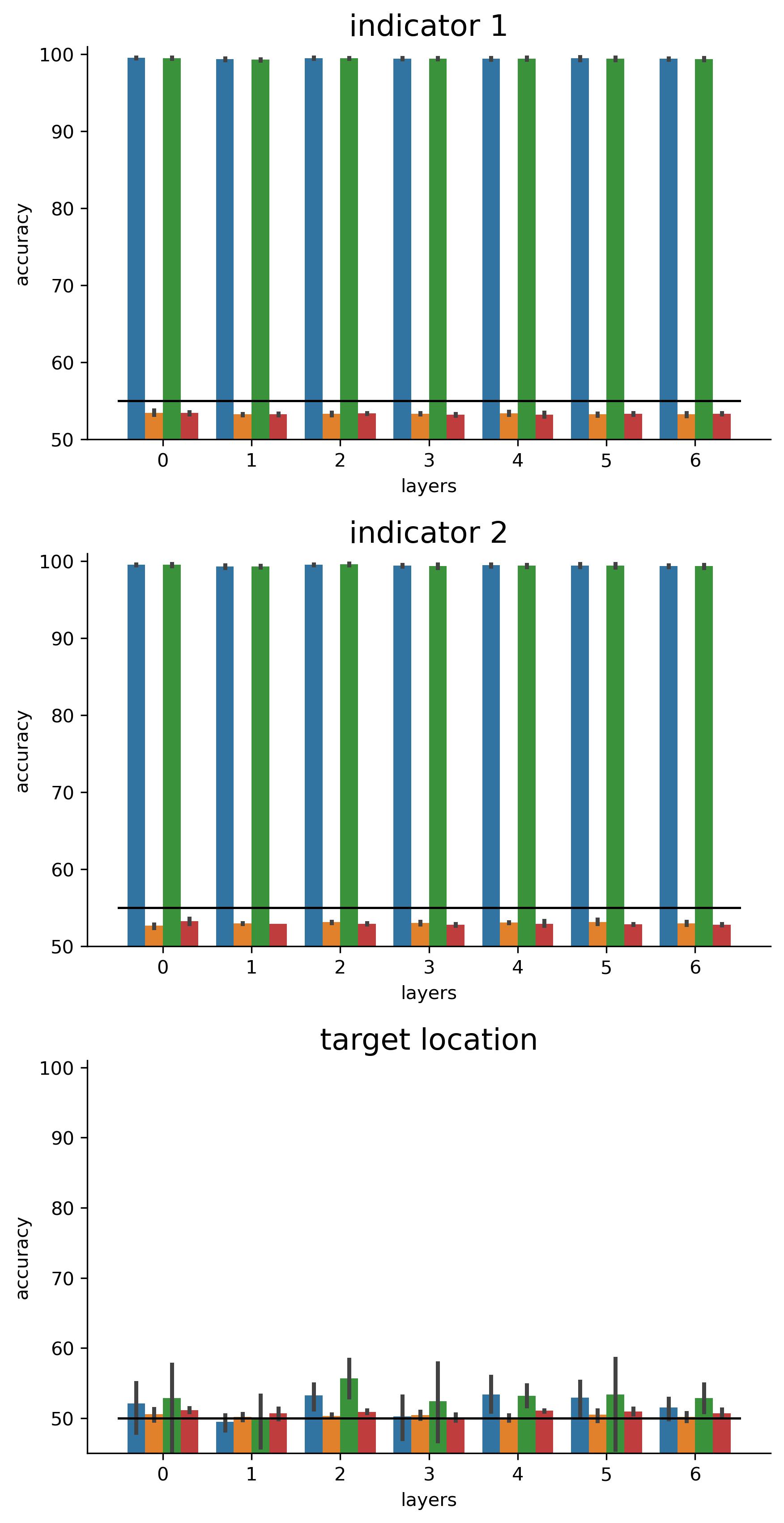
(a) ViT without Eureka-moment

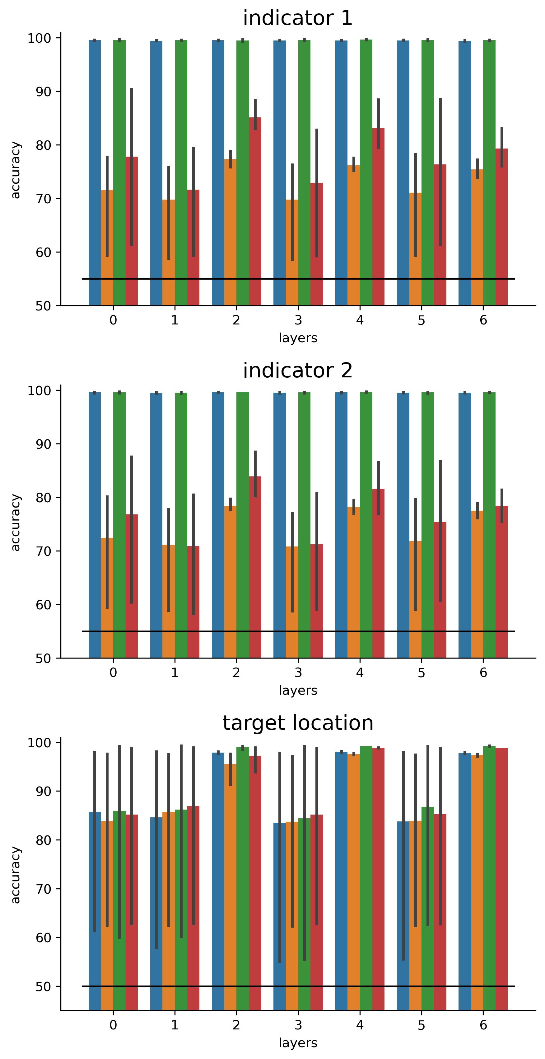
(b) ViT with Eureka-moment

Figure 18: Linear probe for V.

The linear probe results for $V$ look very similar to those for $Q$ and $K$ (see Fig. 18).

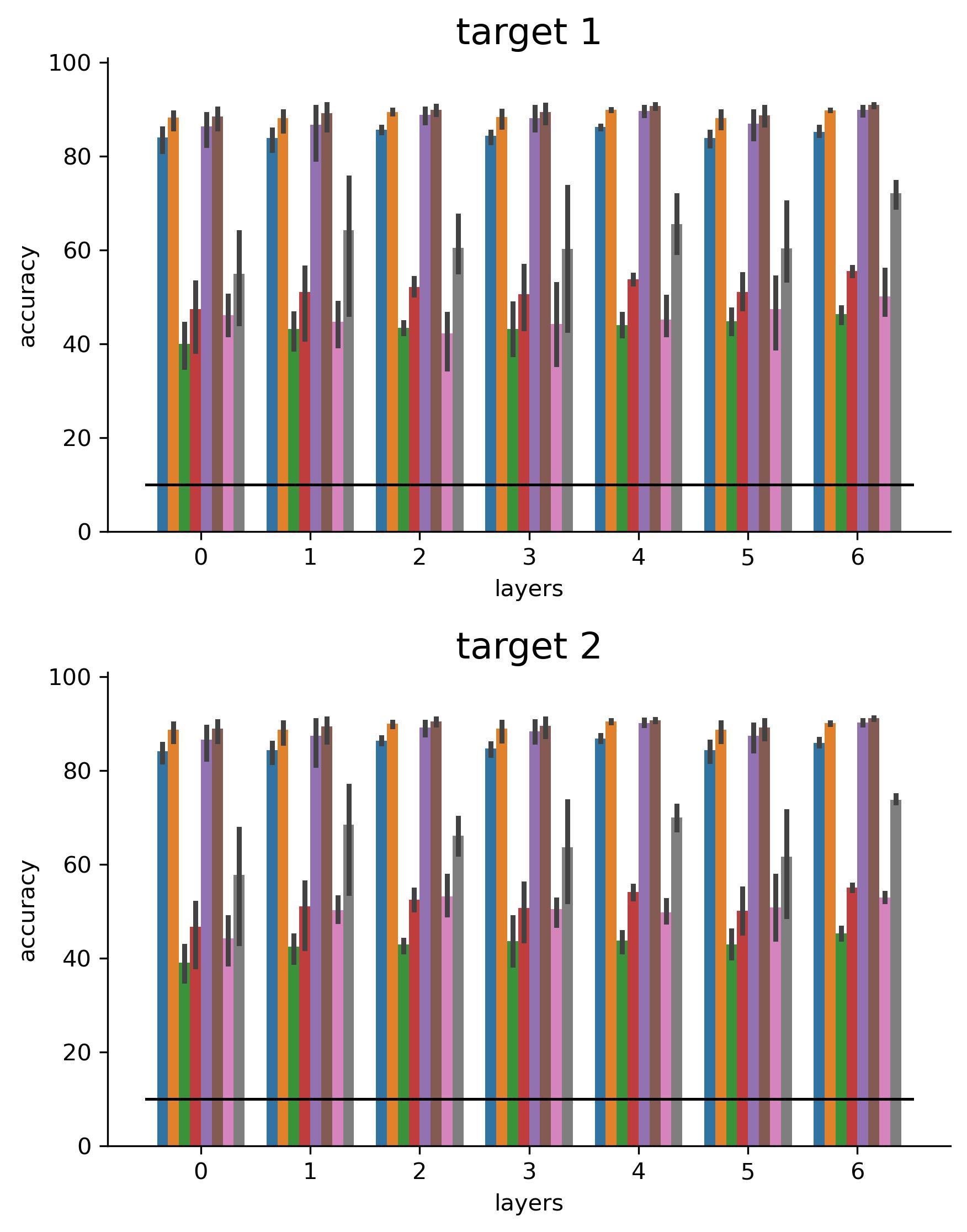
(a) ViT without Eureka-moment

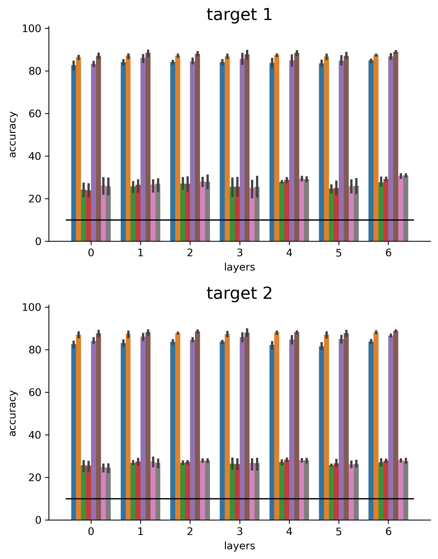
(b) ViT with Eureka-moment

Figure 19: Linear probe for Z with target classification.

Linear probes from $Z$ to targets. Last, we show the linear probe results when predicting the targets from $Z$. As can be seen, from the entire representation, for both ViT with Eureka-moment and Vit without Eureka-moment, target classes can be predicted with high accuracy. Differences can be observed when using only the CLS token. Here, we observe that more target information is in the CLS token of the model without Eureka-moment (see Fig. 19).

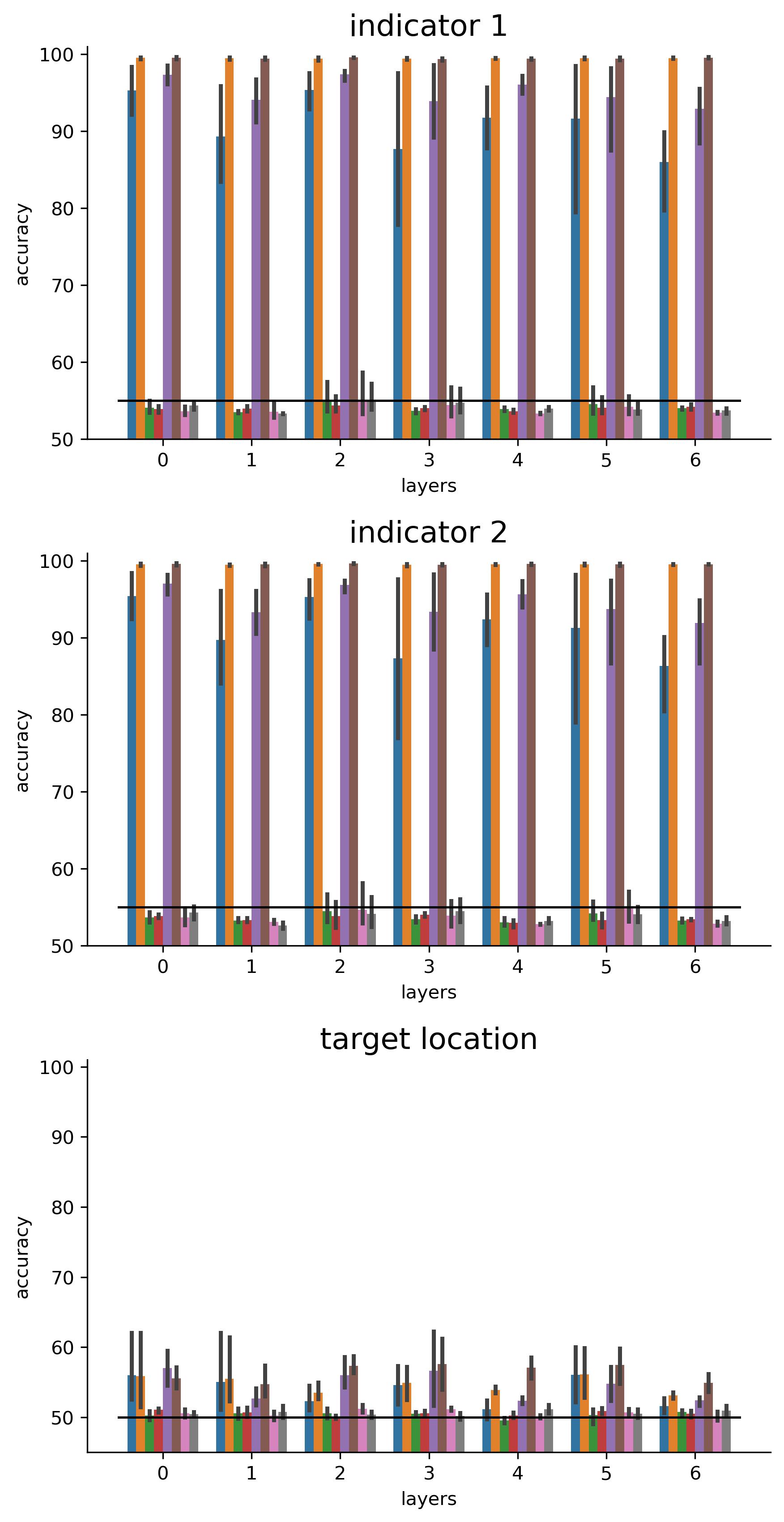
(a) ViT without Eureka-moment

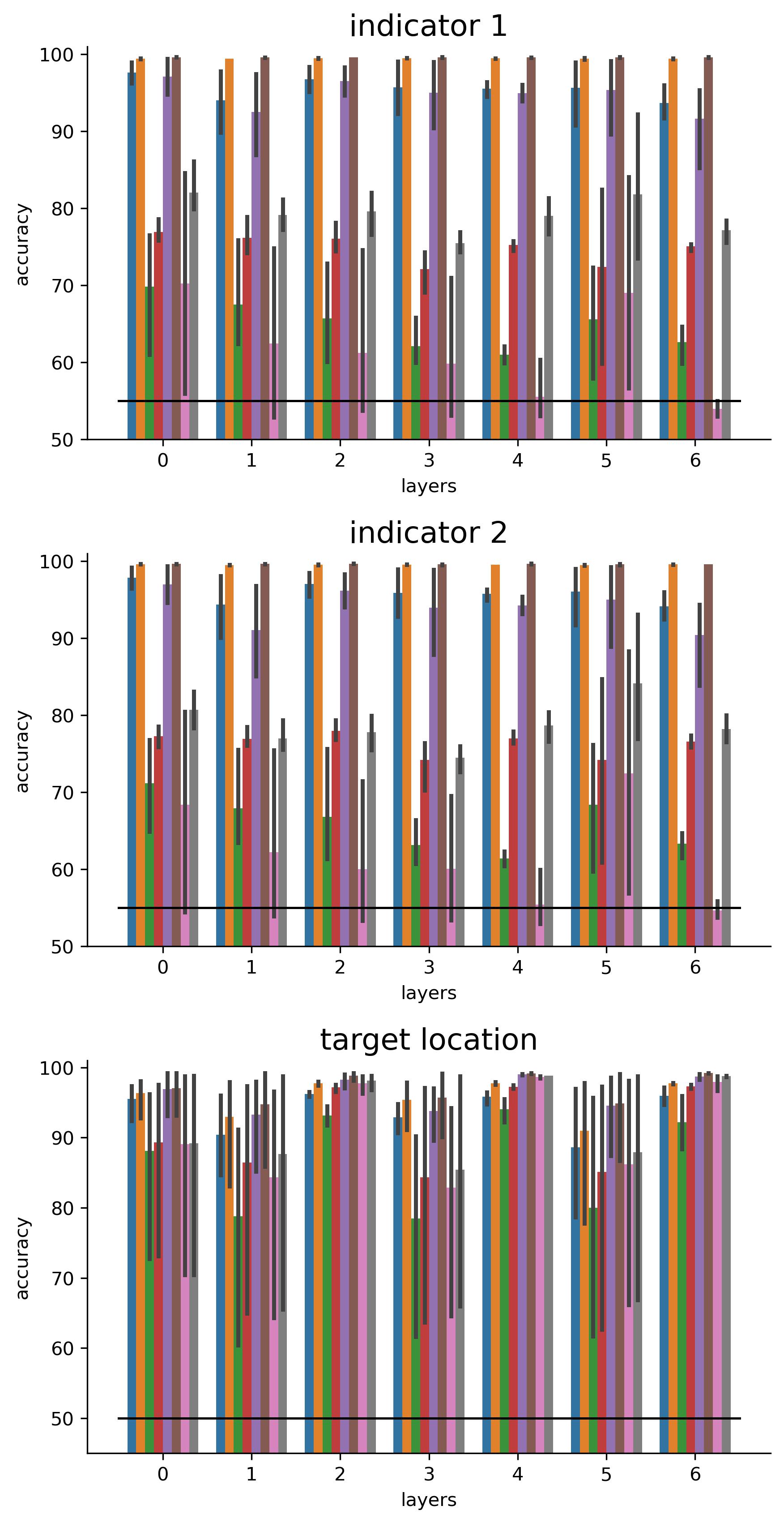
(b) ViT with Eureka-moment

Figure 13: Linear probe results for with $Z$ as input (all layers). This the complete version of Fig. 2. Additionally, we can observe in (b) that layers 2, 3 and 6 contain more target location information than other layers, indicating, that this information can be processed in these layers.

A.7 Main results with standard deviation, ResNet and convergence speed improvements

Due to space and readability constraints we report in the main paper only the mean over all seeds. In Tab. 4 and Tab. 5 we show the same tables including the standard deviation.

Additionally, Tab. 4 and Tab. 5 also provide a comparison to a ResNet9.

Last, for Tab. 4 we report the improved convergence speed as a percentage of the number of training steps to reach 95% of ViT accuracy (averaged only over seeds with Eureka-moments), denoted as “% of steps”. This value is computed only over the fraction of seeds, that actually lead to a higher accuracy than 95% of ViTs accuracy. In the last column, we also report this fraction. Note, that the Eureka-ratio is the maximum possible value for the “95%-ratio”, i.e. for “ViT +Warmup 20” 8/10 seeds have an Eureka-moment. Out of these 8 only 5 reach an accuracy higher than 95% of the ViT accuracy.

Table 4: Main dataset – Comparison of proposed solutions and baselines. This is a complete version of Tab. 1 including standard deviation, and speed improvements. For the main dataset, as described in Fig. 1(a). ER: Eureka-ratio, Acc.: Accuracy, Avg. EE.: average Eureka-epoch. % of steps indicates the % of steps needed to reach 95% of ViTs accuracy. 95%-ratio indicates the ratio of models that actually reached 95% of ViTs accuracy.

		Main Dataset
			Avg. over EMs		Avg. over ViT 95% Acc.
Model	$\tau$	ER $\uparrow$	Acc. $\uparrow$	Avg. EE.	% of steps	95%-ratio
ResNet		10/10	99.40 $\pm$ 0.10	3.00 $\pm$ 00.00	-	-
ViT	$\frac{1}{0.025}$	3/10	89.40 $\pm$ 0.08	174.67 $\pm$ 37.82	84.26	3/10
ViT	$\frac{1}{0.075}$	6/10	90.13 $\pm$ 0.40	181.34 $\pm$ 24.94	86.79	2/10
ViT + WD 0.5	$\sqrt{d_{k}}$	5/10	90.09 $\pm$ 0.27	177.80 $\pm$ 52.30	84.70	5/10
ViT	$\sqrt{d_{k}}$	7/10	89.48 $\pm$ 1.10	207.43 $\pm$ 46.65	100.00	4/10
ViT + Warmup 20	$\sqrt{d_{k}}$	8/10	87.65 $\pm$ 6.48	205.87 $\pm$ 57.05	91.87	5/10
$W_{QKV}$ grad scaling	$\sqrt{d_{k}}$	10/10	87.96 $\pm$ 2.45	119.4 $\pm$ 62.70	73.79	5/10
NormSoftmax	$\sqrt{d_{k}}$	10/10	89.56 $\pm$ 0.65	28.20 $\pm$ 34.85	19.87	10/10
NormSoftmax	$\frac{1}{3}$	10/10	89.18 $\pm$ 0.36	23.50 $\pm$ 08.15	19.25	10/10
ViT	$\frac{1}{3}$	10/10	89.35 $\pm$ 0.28	66.60 $\pm$ 58.55	36.71	10/10
ViT+HT	$\frac{1}{3}\rightarrow\sqrt{d_{k}}$	10/10	89.81 $\pm$ 0.29	74.00 $\pm$ 61.29	39.88	10/10
NormSoftmax + HT	$\frac{1}{3}\rightarrow\sqrt{d_{k}}$	10/10	89.83 $\pm$ 0.41	17.50 $\pm$ 04.84	16.41	10/10

Table 5: No Position Task – Comparison of proposed solutions and baselines. This is a complete version of Tab. 1 including standard deviation for the No position task, as described in Fig. 7(b). $\tau$ not optimized for this task. ER: Eureka-ratio, Acc.: Accuracy, Avg. EE.: average Eureka-epoch.

		No Position Task
			Avg. over EMs
Model	$\tau$	ER $\uparrow$	Acc. $\uparrow$	Avg. EE.
ResNet		4/4	91.27 $\pm$ 0.30	4.25 $\pm$ 00.43
ViT	$\sqrt{d_{k}}$	0/4	-	-
ViT + Warmup 20	$\sqrt{d_{k}}$	1/4	89.55 $\pm$ 0.00	117 $\pm$ 00.00
$W_{QKV}$ grad scaling	$\sqrt{d_{k}}$	0/4	-	-
NormSoftmax	$\sqrt{d_{k}}$	3/4	88.98 $\pm$ 0.55	228.67 $\pm$ 08.22
NormSoftmax	$\frac{1}{3}$	1/4	89.77 $\pm$ 0.00	20.00 $\pm$ 00.00
ViT	$\frac{1}{3}$	1/4	89.68 $\pm$ 0.00	191.00 $\pm$ 00.00
ViT+HT	$\frac{1}{3}\rightarrow\sqrt{d_{k}}$	1/4	88.36 $\pm$ 0.00	242.00 $\pm$ 00.00
NormSoftmax + HT	$\frac{1}{3}\rightarrow\sqrt{d_{k}}$	1/4	90.63 $\pm$ 0.00	19.00 $\pm$ 00.00
ViT 6 heads, depth 4		0/0	-	-

A.8 Transformers learn the prior $p(z)$

Given a task like $p(y|x,z)\cdot p(z|x)$, i.e. the probability of class $y$ given evidence $x$ and the latent variable $z$, we argue, that transformers first learn a prior $p(z)$, ignoring the evidence. Sometimes they fail to unlearn this and pay attention to the evidence. In all previous experiments, the probability of target 1 or target 2 being the target to classify was 0.5. In a setting without 0.5 probability, the transformer should pick the target which is more frequently correct, in case it actually learns the prior $p(z)$ . We test this by changing the probability of the top-right target to be the target location to 0.65. As can be seen in Fig. 14, the transformer initially learns the shortcut of always picking the more likely target.

[]

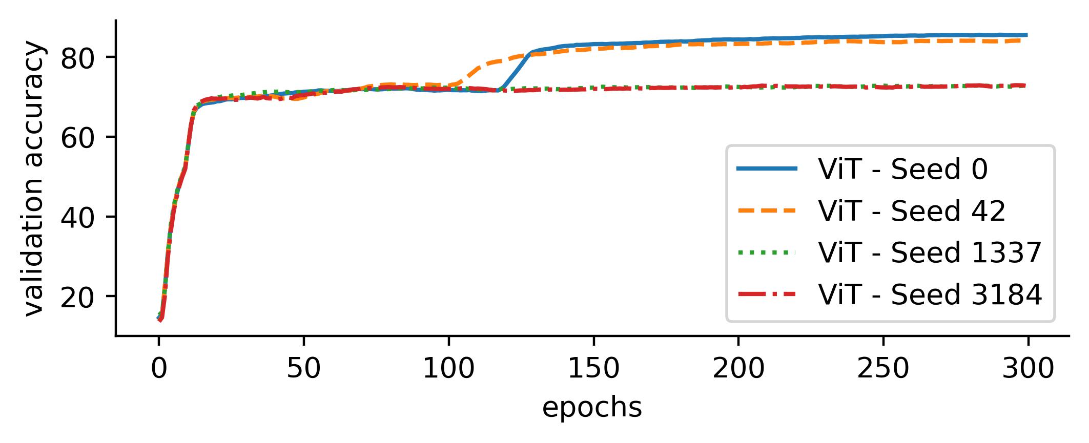
Figure 14: Validation accuracy curves for “main dataset” with changed target probabilities. ViT learns that one target is more likely than the other and learn to always pick this target, as can be seen by the higher plateau accuracy.

A.9 Description of and results on more datasets

In the following we report results on 5 more datasets. The datasets are depicted in Fig. 15.

Cifar task 1. A schematic for this task is shown in Fig. 15(a). The “Cifar task 1” dataset uses Cifar-10 Krizhevsky et al. (2009) images of classes “automobile” and “bird” as indicators. Targets are sampled from fashion MNIST and MNIST. All 4 images are randomly placed on a 4x4 canvas and we apply random colors (red or blue) to the MNIST and fashion MNIST samples. Task 1 is to compare the Cifar-10 classes. If they come from the same class, task 2 is to classify the fashion MNIST sample. If not, the tasks is to classify the MNIST digit. Results are reported in Tab. 6. normal ViT fails in 1/4 cases and Eureka-epoch is usually late. Note, that this task may seem difficult, but differences in color distribution of “bird” and “automobile” simplify the task.

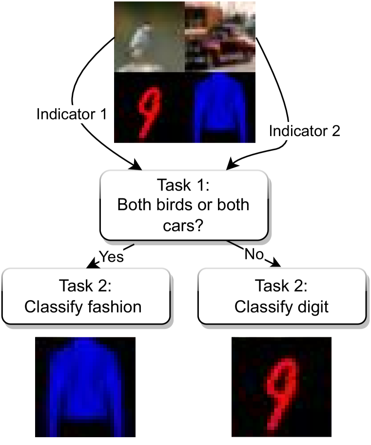
(a) “Cifar task 1”

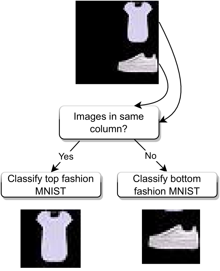
(b) “Top if above”

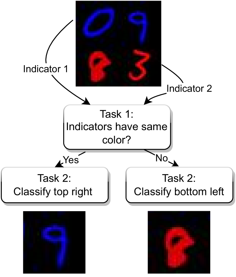
(c) “Same color decision”

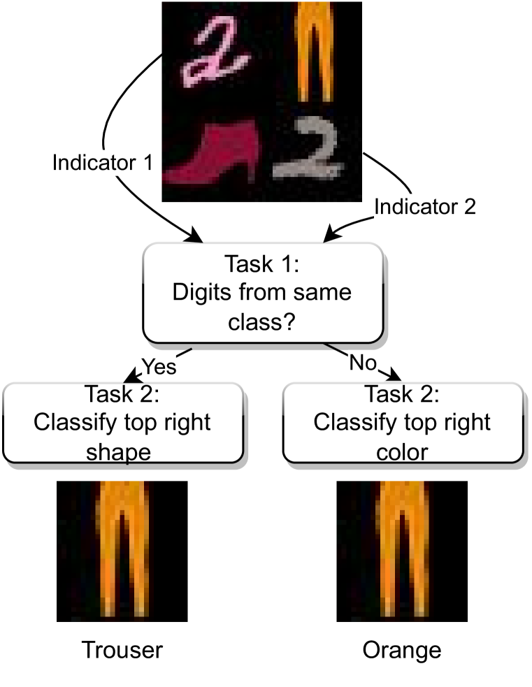
(d) “‘Color or fashion class”

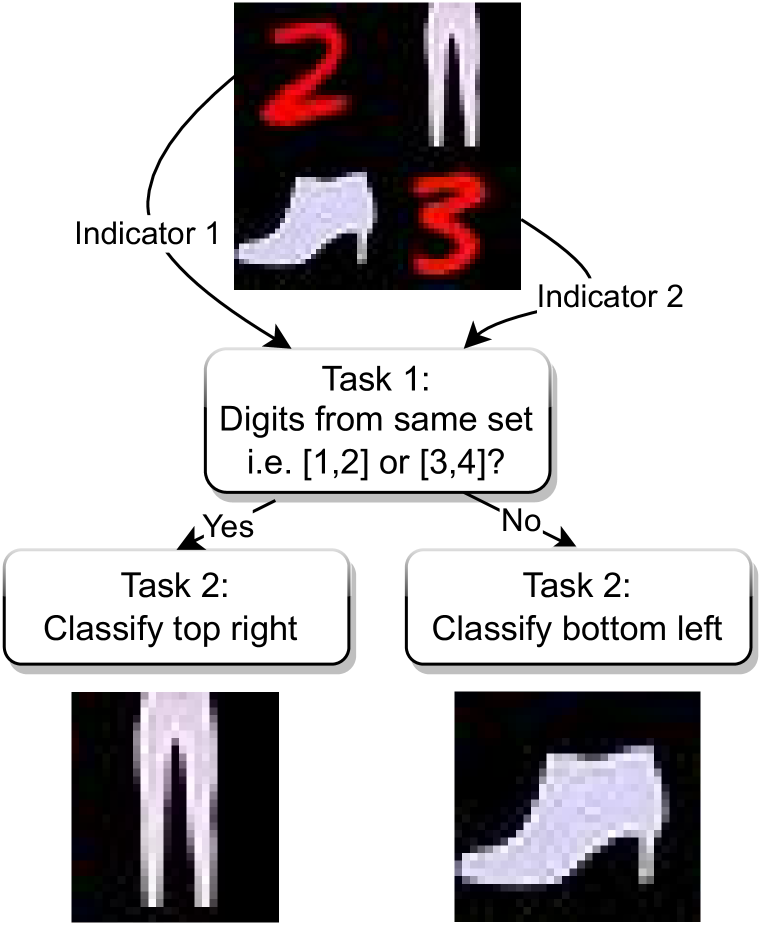
(e) “Digit grouping”

Figure 15: Schematics for additional datasets.

Table 6: Results “Cifar task 1” dataset. $\tau$ not optimized for this task. ER: Eureka-ratio, Acc.: Accuracy, Avg. EE.: average Eureka-epoch.

		Cifar task 1
			Avg. over EMs
Model	$\tau$	ER $\uparrow$	Acc. $\uparrow$	Avg. EE.
ViT	$\sqrt{d_{k}}$	3/4	83.43 $\pm$ 1.83	187.67 $\pm$ 42.46
ViT	$\frac{1}{3}$	4/4	86.86 $\pm$ 0.75	76.50 $\pm$ 08.90
NormSoftmax	$\sqrt{d_{k}}$	4/4	82.89 $\pm$ 0.31	100.0 $\pm$ 27.89

Top if above. The task description is summarized in Fig. 15(b). For data creation we sample 2 images from fashion MNIST and place one in the top row of a 4x4 canvas and the other in the bottom row. The column is selected randomly for both. Task 1 is to check whether the 2 samples are in the same column. If they are task 2 is to classify the top image. If not, the image in the bottom row must be classified. This task is relatively simple, as it removes additional indicators. Instead, relative location of the images is the relevant information to solve task 1. This task is very simple and leads to a low Eureka-epoch for all methods (see 15(b)).

Table 7: Results “Top if above” dataset. $\tau$ not optimized for this task. ER: Eureka-ratio, Acc.: Accuracy, Avg. EE.: average Eureka-epoch.

		Top if above
			Avg. over EMs
Model	$\tau$	ER $\uparrow$	Acc. $\uparrow$	Avg. EE.
ViT	$\sqrt{d_{k}}$	4/4	91.47 $\pm$ 0.13	13.75 $\pm$ 2.19
ViT	$\frac{1}{3}$	4/4	90.38 $\pm$ 0.13	9.5 $\pm$ 1.25
NormSoftmax	$\sqrt{d_{k}}$	4/4	90.84 $\pm$ 0.27	9.25 $\pm$ 1.09

Same color decision task. The task is explained in Fig. 15(b). For data creation we sample only MNIST digits and apply random colors (red or blue) to all digits. If color of the indicators is identical, the top right must be classified and bottom left if not. As can be seen in Tab. 8, this task is again very easy. Color seems to be easily accessible for ViT and ViT has little trouble to compare the indicator colors.

Table 8: Results “Same color decision task” dataset. $\tau$ not optimized for this task. ER: Eureka-ratio, Acc.: Accuracy, Avg. EE.: average Eureka-epoch.

		Same color decision task
			Avg. over EMs
Model	$\tau$	ER $\uparrow$	Acc. $\uparrow$	Avg. EE.
ViT	$\sqrt{d_{k}}$	4/4	98.35 $\pm$ 0.58	91.5 $\pm$ 60.04
ViT	$\frac{1}{3}$	4/4	98.95 $\pm$ 0.10	8.25 $\pm$ 1.48
NormSoftmax	$\sqrt{d_{k}}$	4/4	98.93 $\pm$ 0.03	7.75 $\pm$ 0.43

Color or fashion classifcation. This task is shown in Fig. 15(d). For the creation of the dataset we define 10 random colors, i.e. (brown, blue, yellow, orange, red, green, purple, gray, pink, turquoise) and apply a random color to each target and each indicator sample. For targets we use fashion MNIST samples and indicators are MNIST classes 1 and 2. Task 1 is to compare digits. If they are the same class, the top right fashion sample must be classified. If not, the color of the top right sample must be classified.

Table 9: Results “Color or fashion class” dataset. $\tau$ not optimized for this task. ER: Eureka-ratio, Acc.: Accuracy, Avg. EE.: average Eureka-epoch.

		Color or fashion class
			Avg. over EMs
Model	$\tau$	ER $\uparrow$	Acc. $\uparrow$	Avg. EE.
ViT	$\sqrt{d_{k}}$	4/4	92.85 $\pm$ 0.25	12.00 $\pm$ 3.32
ViT	$\frac{1}{3}$	4/4	92.53 $\pm$ 0.40	20.75 $\pm$ 2.49
NormSoftmax	$\sqrt{d_{k}}$	4/4	92.75 $\pm$ 0.71	11.25 $\pm$ 0.83

Digit grouping. Finally, we make the indicator task more difficult. We follow the same setting as for the “main dataset”, as described in Fig 1(a). However, indicators are not sampled from digits 1 and 2, but from 1, 2, 3 and 4. Task 1 is to find out whether both indicators are smaller or both indicators are larger or equal to 3. I.e. we build indicator sets $[1,2]$ and $[3,4]$ if both indicators are from the same group the top-right image should be classified. As can be seen in Tab. 10, increasing the difficulty of the indicator task quickly makes the dataset too hard. Further optimization of hyper-parameters and architecture are likely to solve the tasks.

Table 10: Results “Digit grouping” dataset. $\tau$ not optimized for this task. ER: Eureka-ratio, Acc.: Accuracy, Avg. EE.: average Eureka-epoch.

		Digit grouping
			Avg. over EMs
Model	$\tau$	ER $\uparrow$	Acc. $\uparrow$	Avg. EE.
ViT	$\sqrt{d_{k}}$	0/4	-	-
ViT	$\frac{1}{3}$	0/4	-	-
NormSoftmax	$\sqrt{d_{k}}$	0/4	-	-

(a) ViT without Eureka-moment

A.10 Experimental setup — Vision Task

We mostly follow the DeiT Touvron et al. (2021) training recipe without distillation. For optimization we use AdamW Loshchilov & Hutter (2019) with default values, i.e. $\beta_{1}=0.9$ and $\beta_{2}=0.999$ and $\epsilon=10^{-8}$. Unless otherwise stated we Warmup the learning rate for 5 epochs from $10^{-6}$ to the maximum learning rate, use a weight decay of 0.05 and train for 300 epochs. We train all models with a batch size of 512, which fits on a single V100, for all the architectures that we considered. Since position and color can be important cues in our datasets we train without data augmentation. We only sample color-noise from a standard normal Gaussian with standard deviation 0.05 for each color channel independently. Color-noise is sampled for each sub-sample (i.e. each indicator and each target) independently and added to the RGB value.

Learning rate schedules for all models. To compare the tested methods and models fairly, we run a search over 9 learning rate schedules with 4 random seeds, each. We anneal the learning rate from a maximum to a minimum using a cosine scheduler. We also use Warmup, as described in the section on training details. The different schedules can be seen in Tab. 11. We pick the schedule that leads to highest Eureka-ratio for each model. In case of a tie we pick the schedule with higher accuracy.

Table 11: Learning rate schedules. We use cosine annealing from “max learning rate” to “min learning rate”.

max learning rate	min learning rate
$10^{-3}$	$10^{-5}$
$10^{-3}$	$5*10^{-6}$
$10^{-4}$	$10^{-5}$
$5*10^{-4}$	$5*10^{-6}$
$5*10^{-4}$	$10^{-6}$
$10^{-4}$	$10^{-6}$
$5*10^{-5}$	$10^{-6}$
$10^{-5}$	$10^{-6}$
$10^{-5}$	$10^{-7}$

Info on taus: In initial experiments we tested for ViT 5 $\tau$, $\tau=\frac{2}{3}$, $\tau=\frac{1}{2}$, $\tau=\frac{1}{3}$, $\tau=\frac{1}{4}$ and $\tau=\frac{1}{5}$. We found $\tau=\frac{1}{3}$, $\tau=\frac{1}{4}$ to work well and did not further optimize them for the different methods. For HT we set the goal temperature to the default $\sqrt{d_{k}}$ and tried also $\frac{1}{2*\sqrt{d_{k}}}$. Further optimizing these parameters for each model and dataset will most likely lead to improvements, but would add very little to a deeper understanding of the Eureka-moments.

A.11 Implementation details NormSoftmax

In practice, $\sigma(\cdot)$ can be defined by arbitrary functions. As highlighted in the background section, the standard deviation is a theoretically motivated choice. Alternatives are discussed by Jiang et al. (2022). In this work, we find the variance to work better for ViT and RoBERTa, while we stick to the standard deviation for the reasoning task.

A.12 Experimental setup – reasoning task

The input of the model is of the form “a b c d =“, where, where $a,b,c,d\in\{0,1,\dots,n\}$. In our experiments, we set $n=11$. We train the transformer on $30\text{\,}\mathrm{\%}$ of the entire set of possible inputs (i.e., $11^{4}=14\,641$ input combinations), that is with a batch size of 4392. The rest is used as test set. We train for 10 000 epochs over five random seeds. We use token embeddings of size of $d=2^{\lceil\log_{2}n\rceil}=16$, four attention heads of dimension of $d/4=4$, $4d=64$ hidden units in the MLP, and learned positional embeddings.

We trained with full batch gradient descent using AdamW (Loshchilov & Hutter, 2019) with a cross-entropy loss. We optimized learning rates via grid search over $[10^{-4},\;10^{-2}]$ on seed 0. Following Nanda et al. (2023) we use a weight decay of 1.

A.13 Slingshot effects on non-reasoning task

We observed that NormSoftmax caused slingshot effects (Thilak et al., 2022) during the convergence phase of some of the training runs but believe this may be due to the interaction of gradients at different scales with adaptive optimizers (Nanda et al., 2023). Since slingshot effects only occur after Eureka-moments, they cannot be the cause for their occurrence. We did not further investigate this observation.

A.14 Experimental Setup RoBERTa

The RoBERTa experiments are based on the Code provided by (Deshpande & Narasimhan, 2020). We follow the data acquisition and preparation strategy of Shoeybi et al. (2019). Thus, we train on the latest Wikipedia dump (downloaded on 08.02.2023). We train a 12 layer RoBERTa model with 12 heads. We use a batch size of 84 and a learning rate of 5e-5.

A.15 Vanishing gradient in the Softmax.

Softmax attention can cause vanishing gradients for $W_{q}$ and $W_{K}$. To see that Softmax attention can result in vanishing gradients it helps to take a look at the gradients of the attention function. Let

$$A(W_{q},W_{k},W_{v},X) =Z$$ (3)

$$A(W_{q},W_{k},W_{v},X) =S\Bigl{(}D\bigl{(}Q(W_{q},X),K(W_{k},X)\bigr{)}\Bigr{)}(W_{v},X),$$ (4)

$$S(D) =\text{Softmax}(D),$$ (5)

$$D(Q,K) =\frac{QK^{T}}{\tau},$$ (6)

$$Q(W_{q},X) =W_{q}X,$$ (7)

$$K(W_{k},X) =W_{k}X,$$ (8)

$$V(W_{v},X) =W_{v}X.$$ (9)

be the attention function, where $W_{k}$, $W_{q}$ and $W_{v}$ are weight matrices, $X$ is the input.

Using the chain rule we get

$$\frac{\partial A}{\partial W_{q}}= \frac{\partial A}{\partial D}\frac{\partial D}{\partial Q}\frac{\partial Q}{\partial W_{q}}$$ (10)

$$\frac{\partial A}{\partial W_{k}}= \frac{\partial A}{\partial D}\frac{\partial D}{\partial K}\frac{\partial K}{\partial W_{k}}.$$ (11)

Since $\frac{\partial D}{\partial Q},\frac{\partial Q}{\partial W_{q}},\frac{\partial D}{\partial K},\frac{\partial K}{\partial W_{k}}$ are constants we only need to look more closely into $\frac{\partial A}{\partial D}$.

$\frac{\partial A}{\partial D}$ is given by $\frac{\partial A}{\partial D}=\frac{\partial S}{\partial D}V$, where $S(D)$ takes the values $S=(s_{1},\dots,s_{n})$. Therefore, to analyze how the gradients $\frac{\partial A}{\partial W_{q}}$ and $\frac{\partial A}{\partial W_{k}}$ behave, we need to analyze the $\frac{\partial S}{\partial D}$, i.e. the Jacobian of the Softmax $S(D)$. It is given by

$$\frac{\partial S}{\partial D}=\begin{pmatrix}s_{1}(1-s_{1})&-s_{1}s_{2}&\dots&-s_{1}s_{n}\\ -s_{2}s_{1}&s_{2}(1-s_{2})&\dots&-s_{2}s_{n}\\ \vdots&\vdots&\ddots&\vdots\\ -s_{n}s_{1}&-s_{n}s_{2}&\dots&s_{n}(1-s_{n})\end{pmatrix}.$$ (12)

It can be easily seen, that almost all entries in the Jacobian are close to 0 whenever a single $s_{i}$ is close to 1 and all others are almost 0.

References

- Ali et al. (2021) Alaaeldin Ali, Hugo Touvron, Mathilde Caron, Piotr Bojanowski, Matthijs Douze, Armand Joulin, Ivan Laptev, Natalia Neverova, Gabriel Synnaeve, Jakob Verbeek, et al. Xcit: Cross-covariance image transformers. Advances in neural information processing systems, 34:20014–20027, 2021.
- Baevski & Auli (2018) Alexei Baevski and Michael Auli. Adaptive input representations for neural language modeling. arXiv preprint arXiv:1809.10853, 2018.
- Barak et al. (2022) Boaz Barak, Benjamin Edelman, Surbhi Goel, Sham Kakade, Eran Malach, and Cyril Zhang. Hidden progress in deep learning: Sgd learns parities near the computational limit. Advances in Neural Information Processing Systems, 2022.
- Chen et al. (2023) Xiangyu Chen, Qinghao Hu, Kaidong Li, Cuncong Zhong, and Guanghui Wang. Accumulated trivial attention matters in vision transformers on small datasets. In Proceedings of the IEEE/CVF Winter Conference on Applications of Computer Vision, pp. 3984–3992, 2023.
- Child et al. (2019) Rewon Child, Scott Gray, Alec Radford, and Ilya Sutskever. Generating long sequences with sparse transformers. arXiv preprint arXiv:1904.10509, 2019.
- Dehghani et al. (2023) Mostafa Dehghani, Josip Djolonga, Basil Mustafa, Piotr Padlewski, Jonathan Heek, Justin Gilmer, Andreas Steiner, Mathilde Caron, Robert Geirhos, Ibrahim Alabdulmohsin, et al. Scaling vision transformers to 22 billion parameters. arXiv preprint arXiv:2302.05442, 2023.
- Deshpande & Narasimhan (2020) Ameet Deshpande and Karthik Narasimhan. Guiding attention for self-supervised learning with transformers. In Findings of the Association for Computational Linguistics: EMNLP 2020, pp. 4676–4686, 2020.
- Dong et al. (2021) Yihe Dong, Jean-Baptiste Cordonnier, and Andreas Loukas. Attention is not all you need: Pure attention loses rank doubly exponentially with depth. In International Conference on Machine Learning, pp. 2793–2803. PMLR, 2021.
- Dufter et al. (2020) Philipp Dufter, Martin Schmitt, and Hinrich Schütze. Increasing learning efficiency of self-attention networks through direct position interactions, learnable temperature, and convoluted attention. In Proceedings of the 28th International Conference on Computational Linguistics, pp. 3630–3636, 2020.
- Geirhos et al. (2020) Robert Geirhos, Jörn-Henrik Jacobsen, Claudio Michaelis, Richard Zemel, Wieland Brendel, Matthias Bethge, and Felix A Wichmann. Shortcut learning in deep neural networks. Nature Machine Intelligence, 2020.
- Gilmer et al. (2023) Justin Gilmer, Andrea Schioppa, and Jeremy Cohen. Intriguing Properties of Transformer Training Instabilities, 2023. To appear.
- Gupta & Berant (2020) Ankit Gupta and Jonathan Berant. Gmat: Global memory augmentation for transformers. arXiv preprint arXiv:2006.03274, 2020.
- Hassani et al. (2021) Ali Hassani, Steven Walton, Nikhil Shah, Abulikemu Abuduweili, Jiachen Li, and Humphrey Shi. Escaping the big data paradigm with compact transformers. arXiv preprint arXiv:2104.05704, 2021.
- Huang et al. (2020) Xiao Shi Huang, Felipe Perez, Jimmy Ba, and Maksims Volkovs. Improving transformer optimization through better initialization. In International Conference on Machine Learning, pp. 4475–4483. PMLR, 2020.
- Jiang et al. (2022) Zixuan Jiang, Jiaqi Gu, and David Z Pan. Normsoftmax: Normalize the input of softmax to accelerate and stabilize training. 2022.
- Kenton & Toutanova (2019) Jacob Devlin Ming-Wei Chang Kenton and Lee Kristina Toutanova. Bert: Pre-training of deep bidirectional transformers for language understanding. In Proceedings of naacL-HLT, volume 1, pp. 2, 2019.
- Krizhevsky et al. (2009) Alex Krizhevsky, Geoffrey Hinton, et al. Learning multiple layers of features from tiny images. 2009.
- LeCun et al. (2010) Yann LeCun, Corinna Cortes, and CJ Burges. Mnist handwritten digit database. ATT Labs [Online]. Available: http://yann.lecun.com/exdb/mnist, 2, 2010.
- Liu et al. (2019) Yinhan Liu, Myle Ott, Naman Goyal, Jingfei Du, Mandar Joshi, Danqi Chen, Omer Levy, Mike Lewis, Luke Zettlemoyer, and Veselin Stoyanov. Roberta: A robustly optimized bert pretraining approach. arXiv preprint arXiv:1907.11692, 2019.
- Liu et al. (2022a) Ziming Liu, Ouail Kitouni, Niklas Nolte, Eric J Michaud, Max Tegmark, and Mike Williams. Towards understanding grokking: An effective theory of representation learning. In Advances in Neural Information Processing Systems, 2022a.
- Liu et al. (2022b) Ziming Liu, Eric J Michaud, and Max Tegmark. Omnigrok: Grokking beyond algorithmic data. In The Eleventh International Conference on Learning Representations, 2022b.
- Loshchilov & Hutter (2019) Ilya Loshchilov and Frank Hutter. Decoupled weight decay regularization. In International Conference on Learning Representations, 2019.
- Millidge (2022) Beren Millidge. Grokking ‘grokking‘, 2022. URL https://www.beren.io/2022-01-11-Grokking-Grokking/.
- Nagatsuka et al. (2021) Koichi Nagatsuka, Clifford Broni-Bediako, and Masayasu Atsumi. Pre-training a bert with curriculum learning by increasing block-size of input text. In Proceedings of the International Conference on Recent Advances in Natural Language Processing (RANLP 2021), pp. 989–996, 2021.
- Nanda et al. (2023) Neel Nanda, Lawrence Chan, Tom Liberum, Jess Smith, and Jacob Steinhardt. Progress measures for grokking via mechanistic interpretability. International Conference on Learning Representations, 2023.
- Noci et al. (2022) Lorenzo Noci, Sotiris Anagnostidis, Luca Biggio, Antonio Orvieto, Sidak Pal Singh, and Aurelien Lucchi. Signal propagation in transformers: Theoretical perspectives and the role of rank collapse. Advances in Neural Information Processing Systems, 35:27198–27211, 2022.
- Olsson et al. (2022) Catherine Olsson, Nelson Elhage, Neel Nanda, Nicholas Joseph, Nova DasSarma, Tom Henighan, Ben Mann, Amanda Askell, Yuntao Bai, Anna Chen, et al. In-context learning and induction heads. arXiv preprint arXiv:2209.11895, 2022.
- Power et al. (2022) Alethea Power, Yuri Burda, Harri Edwards, Igor Babuschkin, and Vedant Misra. Grokking: Generalization beyond overfitting on small algorithmic datasets. arXiv preprint arXiv:2201.02177, 2022.
- Schaeffer et al. (2023) Rylan Schaeffer, Brando Miranda, and Sanmi Koyejo. Are emergent abilities of large language models a mirage? arXiv preprint arXiv:2304.15004, 2023.
- Shen et al. (2023) Kai Shen, Junliang Guo, Xu Tan, Siliang Tang, Rui Wang, and Jiang Bian. A study on relu and softmax in transformer. arXiv preprint arXiv:2302.06461, 2023.
- Shoeybi et al. (2019) Mohammad Shoeybi, Mostofa Patwary, Raul Puri, Patrick LeGresley, Jared Casper, and Bryan Catanzaro. Megatron-lm: Training multi-billion parameter language models using model parallelism. arXiv preprint arXiv:1909.08053, 2019.
- Srivastava et al. (2022) Aarohi Srivastava, Abhinav Rastogi, Abhishek Rao, Abu Awal Md Shoeb, Abubakar Abid, Adam Fisch, Adam R Brown, Adam Santoro, Aditya Gupta, Adrià Garriga-Alonso, et al. Beyond the imitation game: Quantifying and extrapolating the capabilities of language models. arXiv preprint arXiv:2206.04615, 2022.
- Steinhardt (2022) Jacob Steinhardt. Future ml systems will be qualitatively different. https://bounded-regret.ghost.io/future-ml-systems-will-be-qualitatively-different/, 2022. Accessed: 2023-05-07.
- Thilak et al. (2022) Vimal Thilak, Etai Littwin, Shuangfei Zhai, Omid Saremi, Roni Paiss, and Joshua M. Susskind. The slingshot mechanism: An empirical study of adaptive optimizers and the \emph{Grokking Phenomenon}. In Has it Trained Yet? NeurIPS 2022 Workshop, 2022.
- Touvron et al. (2021) Hugo Touvron, Matthieu Cord, Matthijs Douze, Francisco Massa, Alexandre Sablayrolles, and Herve Jegou. Training data-efficient image transformers & distillation through attention. In International Conference on Machine Learning, volume 139, pp. 10347–10357, July 2021.
- Vaswani et al. (2017) Ashish Vaswani, Noam Shazeer, Niki Parmar, Jakob Uszkoreit, Llion Jones, Aidan N Gomez, Łukasz Kaiser, and Illia Polosukhin. Attention is all you need. Advances in neural information processing systems, 30, 2017.
- Wang et al. (2019) Qiang Wang, Bei Li, Tong Xiao, Jingbo Zhu, Changliang Li, Derek F Wong, and Lidia S Chao. Learning deep transformer models for machine translation. arXiv preprint arXiv:1906.01787, 2019.
- Wang et al. (2021) Shulun Wang, Feng Liu, and Bin Liu. Escaping the gradient vanishing: Periodic alternatives of softmax in attention mechanism. IEEE Access, 9:168749–168759, 2021.
- Wei et al. (2022) Jason Wei, Yi Tay, Rishi Bommasani, Colin Raffel, Barret Zoph, Sebastian Borgeaud, Dani Yogatama, Maarten Bosma, Denny Zhou, Donald Metzler, et al. Emergent abilities of large language models. arXiv preprint arXiv:2206.07682, 2022.
- Xiao et al. (2017) Han Xiao, Kashif Rasul, and Roland Vollgraf. Fashion-mnist: a novel image dataset for benchmarking machine learning algorithms. CoRR, abs/1708.07747, 2017. URL http://arxiv.org/abs/1708.07747.
- Xiong et al. (2020) Ruibin Xiong, Yunchang Yang, Di He, Kai Zheng, Shuxin Zheng, Chen Xing, Huishuai Zhang, Yanyan Lan, Liwei Wang, and Tieyan Liu. On layer normalization in the transformer architecture. In International Conference on Machine Learning, pp. 10524–10533. PMLR, 2020.
- Zhai et al. (2023) Shuangfei Zhai, Tatiana Likhomanenko, Etai Littwin, Dan Busbridge, Jason Ramapuram, Yizhe Zhang, Jiatao Gu, and Joshua M Susskind. Stabilizing transformer training by preventing attention entropy collapse. In International Conference on Machine Learning, pp. 40770–40803. PMLR, 2023.