Cousins Of The Vendi Score: A Family Of Similarity-Based Diversity Metrics For Science And Machine Learning

Abstract

Measuring diversity accurately is important for many scientific fields, including machine learning (ML), ecology, and chemistry. The Vendi Score was introduced as a generic similarity-based diversity metric that extends the Hill number of order $q=1$ by leveraging ideas from quantum statistical mechanics. Contrary to many diversity metrics in ecology, the Vendi Score accounts for similarity and does not require knowledge of the prevalence of the categories in the collection to be evaluated for diversity. However, the Vendi Score treats each item in a given collection with a level of sensitivity proportional to the item’s prevalence. This is undesirable in settings where there is a significant imbalance in item prevalence. In this paper, we extend the other Hill numbers using similarity to provide flexibility in allocating sensitivity to rare or common items. This leads to a family of diversity metrics—Vendi scores with different levels of sensitivity—that can be used in a variety of applications. We study the properties of the scores in a synthetic controlled setting where the ground truth diversity is known. We then test their utility in improving molecular simulations via Vendi Sampling. Finally, we use the Vendi scores to better understand the behavior of image generative models in terms of memorization, duplication, diversity, and sample quality.

1 Introduction

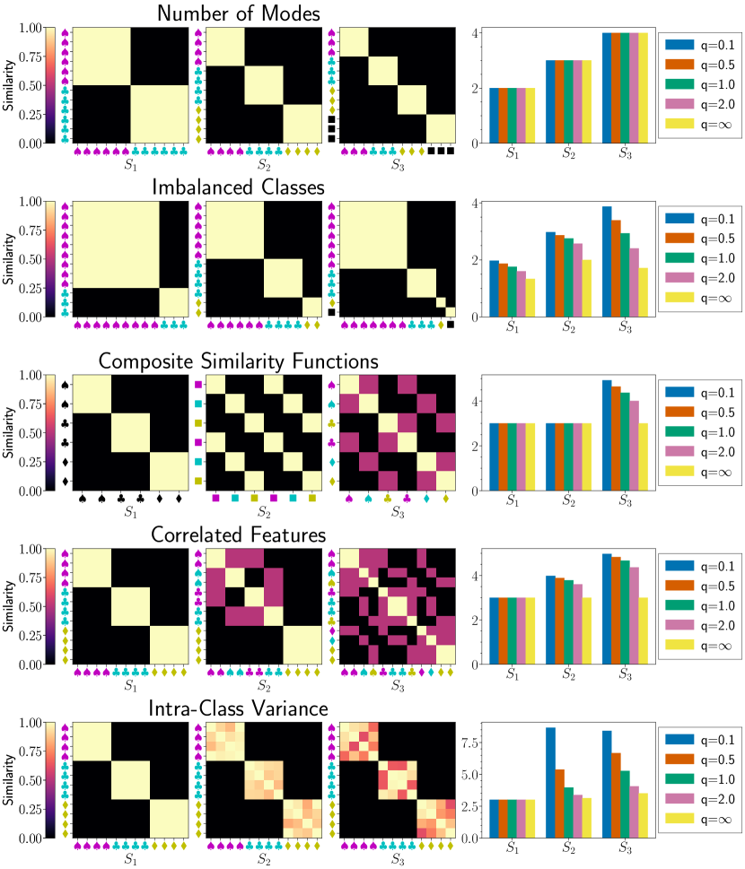
Figure 1: Sensitivity of Different Vendi Scores Under Different Scenarios. Top row: Varying the number of classes under perfect balance. Each Vendi score measures the number of classes exactly; they are effective numbers. Second row: Varying the number of classes under imbalance. Smaller orders $q$ more accurately describe the correct number of modes. Third row: Combining two similarity functions for shape and color. All choices of order $q$ except $q=\infty$ give increases in diversity with the similarity composition. Fourth row: Varying the correlation of shape and color features. As the correlation between shape and color decreases from left to right, all $q$ except $q=\infty$ yield larger Vendi scores. Fifth row: Decreasing the similarity between class members. $q=\infty$ gives a Vendi Score that is resistant to intra-class variance. For smaller $q$s, the Vendi scores increase with larger amounts of variance, although the Vendi score with $q=0.1$ does not change between example $S_{2}$ and $S_{3}$.

Evaluating diversity is a critical problem in many areas of machine learning (ML) and the natural sciences. Having a reliable diversity metric is necessary for evaluating generative models, curating datasets, and analyzing phenomena from the scale of molecules to evolutionary patterns.

Ecologists have long studied the role of diversity in various ecosystems (Whittaker, 1972; Hill, 1973), devising interpretable metrics that capture intuitive notions of diversity. However, these metrics tend to be limited in that they assume the ability to partition elements of an ecosystem into classes or species whose prevalence is known a priori. These metrics are also limited because they don’t account for species similarity. Many have recently argued for the importance of accounting for species similarity to reliably measure diversity (Leinster and Cobbold, 2012). We further argue that a diversity metric that accounts for similarity can be unsupervised, i.e. such a metric doesn’t need to assume the partitioning of elements of an ecosystem into known classes, nor does it need to assume knowledge of class prevalence.

The Vendi Score was recently proposed as a generic unsupervised interpretable diversity metric that accounts for similarity by leveraging ideas from ecology and quantum mechanics (Friedman and Dieng, 2022). It’s been shown useful for measuring the diversity of datasets and generative models (Friedman and Dieng, 2022; Stein et al., 2023; Diamantis et al., 2023), balancing the modes of image generative models (Berns et al., 2023), and accelerating molecular simulations (Pasarkar et al., 2023). However, the Vendi Score accounts for different elements in a given collection according to their prevalence in the collection. This is undesirable in settings where there are large variations in item prevalence, such is the case for many ML settings. We illustrate this failure mode in Figure 1, where the Vendi Score ($q=1$), under class imbalance, fails to separately account for the very rare classes (the black square and the yellow diamond) and lumps them into one class.

Contributions And Main Findings. In this paper, we make several contributions and findings that we summarize below.

• We extend the Vendi Score to a family of diversity metrics, Vendi scores with different levels of sensitivity to item prevalence. The sensitivity is determined by a positive real number $q$, the order of the score. The Vendi scores are based on the Hill numbers in ecology but, unlike Hill numbers, they account for similarity and are unsupervised.

• We showcase the usefulness of the Vendi scores in accelerating the simulation of Alanine dipeptide, a well-studied benchmark molecular system. We find that the choice of $q$ can prioritize dynamics along certain axes, which can improve mixing and convergence.

• We show how the scores can be used to better evaluate and understand the behavior of generative models. We study the Vendi scores jointly with several metrics used in ML to evaluate memorization, diversity, coverage, and sample quality. Our results reveal that generative models with a high human error rate or low Fréchet Distance (FD) and Kernel Distance (KD)—i.e. those generative models that tend to produce samples that human evaluators cannot distinguish from real data—are those that memorize training samples and create duplicates around the memorized training samples. This finding calls for the need to pair sample quality metrics with a metric that reliably measures duplication or memorization and a metric that measures diversity effectively. We recommend pairing sample quality metrics with a Vendi score of small order $(q\in[0.1,0.5])$ for diversity and the Vendi score of infinite order for duplication and memorization. Indeed, the Vendi score with infinite order is the most sensitive to duplicates and is strongly correlated with $C_{T}$-modified, a metric used to measure memorization, whereas Vendi scores of small order are more sensitive to rarer items and can effectively reflect diversity.

• We found the scores to be strongly correlated, positively or negatively, with many existing metrics used to measure memorization and coverage. Those metrics rely on training data. Our findings suggest the Vendi scores provide the ability to indirectly evaluate memorization and coverage without relying on training data. This capability becomes even more important in privacy settings and as training datasets become more and more closed-source.

2 Related Work

Several diversity metrics have been proposed in ML and ecology.

Diversity metrics in ML . ML researchers often use some form of average pairwise similarity to quantify diversity, e.g. pairwise-BLEU (Shen et al., 2019) and D-Lex-Sim (Fomicheva et al., 2020) for text data or IntDiv for molecular data (Benhenda, 2017). Average similarity computations have been scaled from squared complexity to linear complexity in the size of the collection to be evaluated for diversity, enabling the assessment of the diversity of very large chemical databases (Miranda-Quintana et al., 2021; Chang et al., 2022b; Rácz et al., 2022). However, as discussed in Friedman and Dieng (2022), average similarity can fail to effectively capture diversity, even in simple scenarios, e.g. it can score two populations with the same number of components/species but different levels of per-component variance the same.

Other metrics used to evaluate diversity, especially in computer vision, include recall (Sajjadi et al., 2018) and Fréchet Inception distance (FID) (Heusel et al., 2017). However, these metrics are less flexible as they rely on a reference distribution, and in the case of FID, additionally require the availability of a pre-trained network.

Yet other ways of measuring or enforcing diversity have been considered in active learning and experimental design settings (Nguyen and Garnett, 2023; Maus et al., 2022). For example Nguyen and Garnett (2023) enforce diversity via a diminishing returns criterion for multiclass active search, penalizing multiple explorations of the same class through a concave utility function. This yields improved results in multiclass active search. However, the approach is domain-specific and targets diversity indirectly. Several other works have studied diversity in the framework of Bayesian optimization (Maus et al., 2022) or evolutionary algorithms (Mouret and Clune, 2015; Vassiliades et al., 2017; Pugh et al., 2016).

Diversity metrics in Ecology.  Ecologists have long been interested in quantifying diversity and have developed several metrics to assess the diversity of ecological systems. Some of the most ubiquitously used metrics in ecology are arguably the Hill numbers (Hill, 1973) and the triplets alpha diversity, beta diversity, and gamma diversity (Whittaker, 1972).

Hill numbers have been shown to be the only family of diversity metrics that satisfy the axioms of diversity (Leinster and Cobbold, 2012). Hill numbers, although interpretable and grounded in intuitive notions of diversity, have important shortcomings that limit their use: (1) they assume some concept of classes and an ability to classify samples within classes (2) they assume knowledge of an abundance vector $p$ quantifying the number of elements in each class and finally (3) they ignore similarity between elements.

Gamma diversity measures the total diversity of an ecosystem spanning some space. Whittaker (1972) intuited that such a diversity metric should account for both the local diversity measured over individual sites spanning a narrower region of the space (or alpha diversity) and the differentiation among the different sites (or beta diversity). These diversity indices have the same limitations as the Hill numbers mentioned above.

The Vendi Score.  The Vendi Score aims to alleviate many of the challenges faced by the commonly employed metrics in ML and ecology. It is interpretable, reference-free, and satisfies the same axioms of diversity as the Hill numbers (Friedman and Dieng, 2022). Furthermore, unlike the Hill numbers, the Vendi Score accounts for similarity and doesn’t require knowledge of class prevalence.

In a recent extensive evaluation study for image generative models, Stein et al. (2023) used the Vendi score of order $q=1$ and found it to work more effectively as a measure of per-class diversity. In this paper, we show that by using different orders $q$ of the Vendi score, we can gain useful insights into the global diversity of generative model outputs.

3 Hill Numbers And Ecological Diversity

Consider a probability distribution ${\mathbf{p}}=({\textnormal{p}}_{1},\dots,{\textnormal{p}}_{S})$ on a space ${\mathcal{X}}=\left\{1,\dots,S\right\}$. Ecologists refer to each member of ${\mathcal{X}}$ as a species and to the individual probability $p_{i}$ as the relative abundance of the $i^{\text{th}}$ species in ${\mathcal{X}}$. Ecologists have proposed a number of axioms that a diversity metric should satisfy to match intuitions Leinster and Cobbold (2012):

1. Effective number. Diversity is defined as the effective number of species in a population, ranging between $1$ and $|{\mathcal{X}}|$. A population containing $N$ equally abundant, completely dissimilar species should have a diversity score of $N$. If all species are identical, the diversity should be minimized and equal to $1$.

2. Partitioning. Suppose a population is partitioned into subpopulations, with no species shared between subsets, and the species in each subset completely dissimilar from the species in any other subset. Then the diversity of ${\mathcal{X}}$ should be entirely determined by the diversity and size of each subpopulation.

3. Identical species. If two species are identical, then merging them into one should leave the diversity of the population unchanged.

4. Monotonicity. When the similarities between species are increased, diversity should decrease.

5. Permutation symmetry. Diversity should be unchanged by changing the order in which the species are listed.

Historically, most ecological diversity indices have not accounted for species similarity, making the assumption that all species are completely dissimilar and defining diversity only in terms of the relative abundance ${\mathbf{p}}$. In this setting, Chapter 7 of Leinster (2020) shows that the only metrics satisfying the axioms described above are the Hill numbers. The Hill number ${\mathcal{D}}_{q}$ of order $q$ is the exponential of the Renyi entropy ${\mathcal{H}}_{q}$ of order $q$,

$${\mathcal{H}}_{q}({\mathbf{p}}) =\frac{1}{1-q}\log\sum_{i\in\text{supp}({\mathbf{p}})}p_{i}^{q}\quad\text{and}\quad{\mathcal{D}}_{q}({\mathbf{p}})=\exp\left({\mathcal{H}}_{q}({\mathbf{p}})\right).$$ (1)

Here $\text{supp}({\mathbf{p}})$ denotes the set of indices $i$ for which $p_{i}>0$ and $q\geq 0$ determines the relative weight assigned to rare or common items. With $q=0$, all species are given equal weight and ${\mathcal{D}}_{0}({\mathbf{p}})$ is equal to the size of the support. This is an uninformative measure of diversity. More interesting diversity indices correspond to $q\neq 0$, with $q=1$ and $q=\infty$ corresponding to special limit cases. Indeed, the Hill number of order $q=1$ is the exponential of the Shannon entropy of ${\mathbf{p}}$,

$${\mathcal{D}}_{1}({\mathbf{p}}) =\exp\left(-\sum_{i\in\text{supp}({\mathbf{p}})}p_{i}\log p_{i}\right)$$ (2)

and weighs each species in proportion to its prevalence. The other interesting Hill number is also a limit, the Hill number of infinite order,

$${\mathcal{D}}_{\infty}({\mathbf{p}}) =\exp(-\log\max_{i}p_{i})=\frac{1}{\max_{i}p_{i}}$$ (3)

which assigns all the weight to the most common species. For $q\not\in\left\{0,1,\infty\right\}$, the behavior depends on whether $q$ is less than $1$ or greater than $1$. Values of $q$ smaller than $1$ assign higher weight to rare species whereas large values of $q$ assign higher weight to common species.

Despite their popularity in ecology, Hill numbers have shortcomings that limit their use beyond ecology: they make the strong assumption that species prevalence is known and don’t account for species similarity.

4 Cousins Of The Vendi Score: Extending Hill Numbers Using Similarity

How can we lift the limitations of the Hill numbers mentioned above and extend their applicability?  Friedman and Dieng (2022) provide a solution for $q=1$, drawing ideas from quantum statistical mechanics. Indeed, the von Neumann entropy $\mathcal{H}(\rho)$ for a quantum system with density matrix $\rho$ is of the same form as the Hill number of order $1$,

$$\mathcal{H}(\rho) =-\text{tr}(\rho\log\rho)=-\sum_{i}\lambda_{i}\log\lambda_{i}$$ (4)

where the $\lambda_{i}$s are the eigenvalues of $\rho$. Replacing the density matrix with a normalized similarity matrix of species yields the Vendi Score:

$$\text{VS}({\mathbf{x}},\mathbf{k}) =\exp\left(-\text{tr}\left(\frac{K_{{\mathbf{x}}}}{N}\log\frac{K_{{\mathbf{x}}}}{N}\right)\right)=\exp\left(-\sum_{i}\lambda_{i}\log\lambda_{i}\right)$$ (5)

where $\mathbf{k}(\cdot,\cdot)$ is a user-defined similarity function that induces a similarity matrix $K_{{\mathbf{x}}}$ over the species and the $\lambda_{i}$s are the eigenvalues of $\frac{K_{{\mathbf{x}}}}{N}$.

In this paper, we provide a theorem that relates the eigenvalues of a normalized similarity matrix to item prevalence and use this result to extend the Vendi Score to the other Hill numbers.

Theorem 4.1.

[The Similarity-Eigenvalue-Prevalence Theorem] Let $({\mathbf{x}}_{1},\dots,{\mathbf{x}}_{N})$ denote a collection of elements, where each ${\mathbf{x}}_{i}=({\mathbf{x}}_{i1},\dots,{\mathbf{x}}_{iM_{i}})$ contains a unique element repeated $M_{i}$ times, i.e. ${\mathbf{x}}_{ij}={\mathbf{x}}_{ik}$ for all $j,k\in\left\{1,\dots,M_{i}\right\}$. Define $C=\sum_{i=1}^{N}M_{i}$. Let ${\mathbf{K}}\in\mathbb{R}^{C\times C}$ denote a kernel matrix such that ${\mathbf{K}}({\mathbf{x}}_{i\bullet},{\mathbf{x}}_{j\bullet})=1$ when $i=j$ and $0$ otherwise, $\forall i,j\in\left\{1,\dots,N\right\}$. Denote by $\tilde{{\mathbf{K}}}=\frac{{\mathbf{K}}}{C}$ the normalized kernel. Then $\tilde{{\mathbf{K}}}$ has exactly $N$ non-zero eigenvalues $\lambda_{1},\dots,\lambda_{N}$ and $\lambda_{i}=\frac{M_{i}}{C}$ $\forall i\in\left\{1,\dots,N\right\}$.

Proof.

A complete proof of this theorem can be found in the appendix. ∎

The theorem states that under the assumption that members of different species are completely dissimilar—this is the same assumption made in the computation of the Hill numbers— there are as many nonzero eigenvalues of the species similarity matrix as there are species and that these eigenvalues are exactly equal to the prevalence of the different species. This theorem therefore provides a recipe for recovering the different Hill numbers exactly using the similarity-based construct the Vendi Score is based on.

The benefit of computing the Hill numbers using the same similarity-based approach as the Vendi Score is it hints at the possibility of not needing to assume knowledge of species prevalence. Furthermore, the assumption of complete dissimilarity between species is strong and limits the Hill numbers’ applicability. The similarity-based approach described above readily allows us to lift that assumption, by simply replacing the zero entries in the similarity matrix with a user-defined similarity function between species.

Endowed with Theorem 4.1, we can safely transition from Hill numbers—diversity indices that assume knowledge of species prevalence and that don’t account for species similarity—to Vendi scores, diversity indices that don’t assume knowledge of species prevalence and that effectively account for species similarity. We denote by $\text{VS}_{q}({\mathbf{x}},{\mathbf{k}})$ the Vendi score of order $q$ for the collection ${\mathbf{x}}$ under similarity function ${\mathbf{k}}(\cdot,\cdot)$ and define,

$$\text{VS}_{q}({\mathbf{x}},{\mathbf{k}}) =\exp\left(\frac{1}{1-q}\log\sum_{i\in\text{supp}(\lambda({\mathbf{x}},{\mathbf{k}}))}\lambda_{i}^{q}({\mathbf{x}},{\mathbf{k}})\right)$$ (6)

Here $\lambda({\mathbf{x}},{\mathbf{k}})$ denotes the set of eigenvalues of the normalized similarity matrix induced by the input similarity function ${\mathbf{k}}(\cdot,\cdot)$, and $\text{supp}(\lambda({\mathbf{x}},{\mathbf{k}}))$ denotes the indices for the nonzero eigenvalues.

Figure 1 shows the behavior of the Vendi scores under different scenarios. The figure considers collections composed of elements with different shapes and colors. The scores are computed using a similarity function that assigns $1$ to elements with the same shape and color, $0.5$ to elements that have either the same shape or the same color, and $0$ to completely distinct elements. In the figure, we see that the Vendi Score ($q=1$), under class imbalance, fails to separately account for the very rare classes (the black square and the yellow diamond) and lumps them into one class. The Vendi scores with orders smaller than $1$ are more sensitive to those rare classes and accurately measure diversity under class imbalance. The figure also shows Vendi scores with smaller orders to be more reliable under the presence of small variations within different classes.

The Vendi scores have several desiderata beyond the ones we mentioned earlier. Indeed, they enjoy the same axioms as the Hill numbers and are therefore interpretable diversity scores that can be used to study diversity, e.g. in ecological systems. More importantly, the Vendi scores are differentiable, which makes them amenable to gradient-based methods in machine learning and science. This differentiability enables us to go beyond simply evaluating diversity to effectively enforcing diversity, by embedding the scores into objective functions of interest.

Enforcing diversity. Enforcing diversity has benefits in molecular simulations as shown by Pasarkar et al. (2023), but also in many areas of machine learning, e.g. active learning and experimental design (Maus et al., 2022; Nguyen and Garnett, 2023), generative modeling (Dieng et al., 2019), and reinforcement learning (Eysenbach et al., 2018).

Enforcing diversity with average similarity may be ineffective as average similarity fails to capture heterogeneity in data, e.g. variances between members of the same species. We refer the reader to Friedman and Dieng (2022) for examples illustrating the limitations of average similarity as a diversity metric.

Enforcing diversity with other existing diversity metrics such as FID, KID, recall, and coverage is currently computationally impossible. Indeed, these metrics are either non-differentiable or may be challenging to optimize as they require querying large pre-trained networks at each optimization iteration.

The Vendi scores are differentiable interpretable diversity indices that can be used to effectively enforce diversity. In section 5 we use the scores within Vendi Sampling to enforce diversity and study their effectiveness for accelerating molecular simulations.

Computation. Computing the Vendi scores requires finding the eigenvalues of an $N\times N$ normalized similarity matrix. This has complexity ${\mathcal{O}}(N^{3})$ which is computationally costly for large collections. Fortunately, Rayleigh-Risz provides a way to reduce computational cost. Consider a collection of size $N$ and denote by $\tilde{K}$ its normalized similarity matrix. Let $V\in\mathbb{R}^{N\times m}$ be an orthogonal matrix, with $m<<N$. We can compute the eigenvalues of $\tilde{K}$ by computing the eigenvalues of $V^{*}\tilde{K}V$, which is an $m\times m$ matrix.

There are different ways to choose the orthogonal matrix $V$, each leading to a different scaling strategy. For very large collections, choosing $V$ to be a binary orthogonal matrix is equivalent to subsampling $m$ elements of the collection and approximating the Vendi scores using that subset. This would have ${\mathcal{O}}(m^{3})$ complexity, which is efficient for $m<<N$, and would allow to trade-off accuracy with computational cost since $m$ is determined by the user. When embeddings are readily available for the elements in the collection, e.g. Inceptionv3 or DINOv2 embeddings for images, we can perform a Gram-Schmidt orthogonalization of the embedding matrix of the elements of the collection to define $V$. We would then use V as described above to compute the Vendi scores. This would have complexity ${\mathcal{O}}(N^{2}m)$—the same complexity as the computation of metrics such as FID—and has the benefit to extend the covariance trick mentioned in  Friedman and Dieng (2022) to similarity functions beyond cosine similarity.

5 Empirical Study

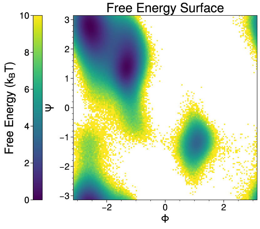
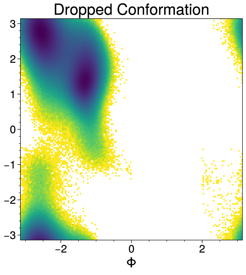
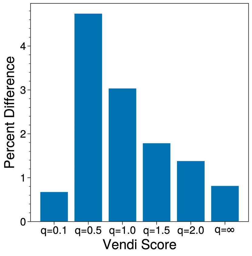
Figure 2: Sensitivity of different Vendi scores to missing Alanine Dipeptide conformation. Left: Ramachandran plot from an unbiased simulation of Alanine Dipeptide plotted against the two dihedral angles $\phi,\psi$. Center: Ramachandran plot after removing the left-handed conformation. Right: The percent difference for different Vendi scores between samples from the original simulation and samples missing the left-handed state. Vendi scores are calculated using $20,000$ molecules from each set of samples using an invariant RBF Kernel with $\gamma=1$.

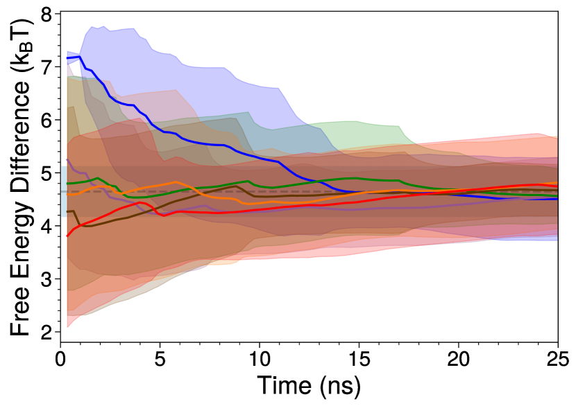
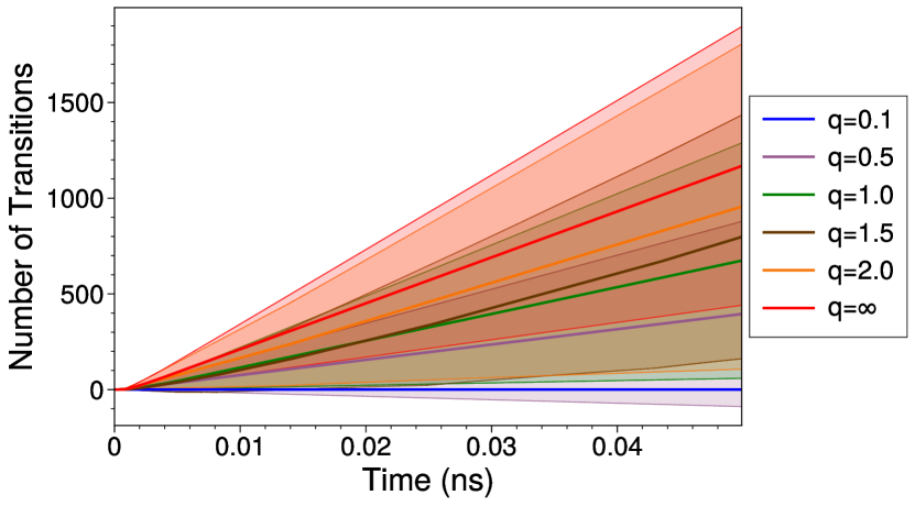
Figure 3: Behavior of the Vendi scores for sampling Alanine Dipeptide. Left: Convergence of Vendi sampling under different scores over 25 ns of simulation to the free energy difference estimated from long unbiased simulations (dashed gray line). Right: Number of transitions for each score in and out of the left-handed state over the course of the first 50 ps of simulation. Shaded regions represent uncertainty over 10 trials.

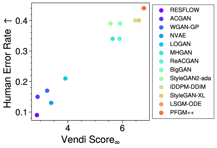
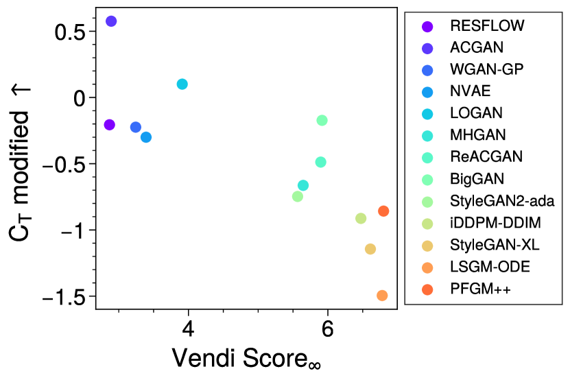
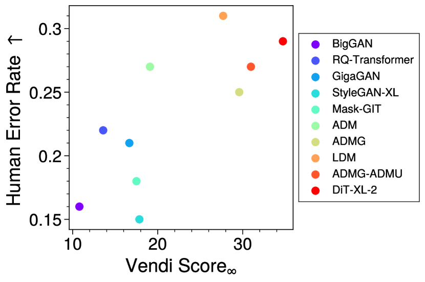
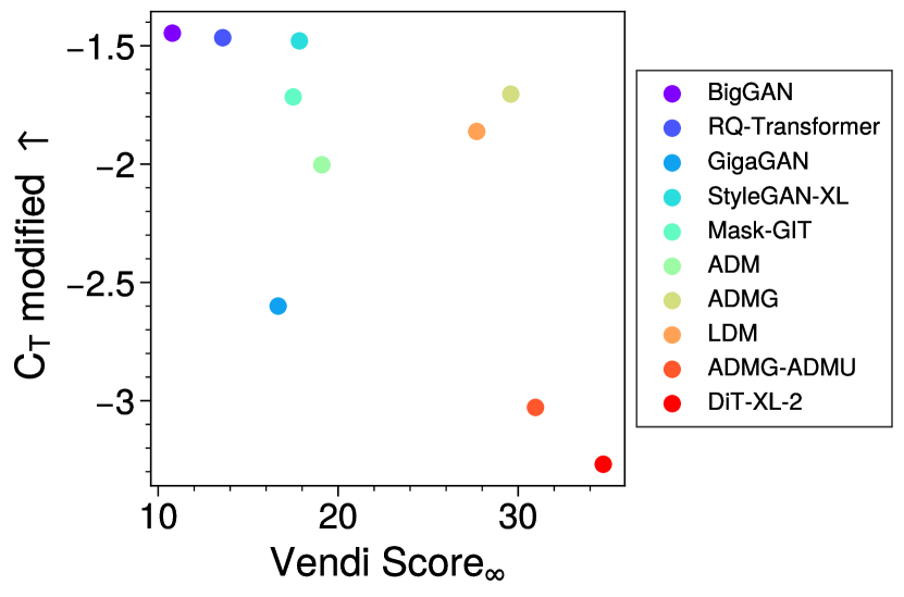
Figure 4: Vendi scores correlate strongly with human evaluation and memorization scores on CIFAR-10 and Imagenet256. Left: Human classification error rate vs. Vendi Score_∞ for models trained on CIFAR-10 (Top) and Imagenet256 (Bottom). Right: $C_{T}$-modified vs. Vendi Score_∞ for models trained on CIFAR-10 (Top) and Imagenet256 (Bottom).

5.1 Application To Vendi Sampling

Molecular simulations through Langevin Dynamics are often plagued by slow mixing times between metastable states. A recent alternative approach, Vendi Sampling, was developed to improve the speed at which these simulations can be performed  (Pasarkar et al., 2023). In Vendi Sampling, a collection of molecular replicas are evolved over time using Langevin Dynamics, with an additional diversity penalty term, called the Vendi force, given by the gradient of the logarithm of the Vendi score. We aim to study how the choice of order $q$ affects the behavior of the Vendi force and the convergence of Vendi Sampling. We analyze convergence by looking at free energy differences.

In order to provide an unbiased estimate of this quantity, we switch the coefficient of the Vendi force to $0$ after a specified number of steps. We only analyze samples taken when this coefficient is $0$.

We can measure the relative probabilities of each state by performing a long unbiased simulation. We perform simulations in OpenMM (v. 8.0) (Eastman et al., 2017), following the experimental setup of  Pasarkar et al. (2023). We used a time step of $2.0\,\mathrm{fs}$ and a collision frequency of $1.0\mathrm{ps}^{-1}$. We establish baselines by running 10 simulations of $100\,\mathrm{ns}$ with $32$ replicas.

To calculate the Vendi scores, we use a Gaussian Radial Basis Function (RBF) kernel $k(x,x^{\prime})=\exp\left(-\gamma\|\mathbf{x}-\mathbf{x}^{\prime}\|^{2}\right)$ where $\gamma$ is a hyperparameter of choice. We also require that the kernel be invariant to various rigid-body transformations, including translations and rotations. We follow the method outlined in Jaini et al. (2021) for computing invariant coordinates. The invariant coordinates are passed into the RBF kernel, from which we can compute the Vendi scores.

We first look to see how sensitive each Vendi score is in detecting Ala2 conformations. We focus on the left-handed state (defined by $0<\phi<2$), which constitutes $\approx 1\%$ of all samples in the reference simulations. We compare Vendi scores from samples from all conformation to samples that are not in the left-handed state. We find that for extreme values of $q$, the score is relatively unaffected, whereas for $q=0.5$ and $q=1$, there is a significant change in the Vendi score (Figure 2). In Figure 1, $q=0.1$ can detect imbalanced classes, but it cannot detect when the intra-class variance changes between non-zero values. This result, combined with Figure 2, suggests that the small values of $q$ can only detect rare classes when there is not a large amount of intra-class diversity, as there would be for Ala2 conformations. Figure 1 also demonstrates that Vendi Score_∞ only detects the presence of large classes, so it is not surprising that it is insensitive to missing the small left-handed state.

We further test the behavior of these scores in Vendi Sampling for Ala2 (Figure 3). We evaluate convergence using the boundary of $\phi=0$. Hyperparameters are tuned for each choice of score via grid search. We find that for most choices of order $q$, the sampling method converges within $0.4k_{B}T$ of the estimated free energy difference within the first $5$ns of simulation, while the Vendi score with $q=0.1$ is slower to converge. Interestingly, unlike in the Double Well system (see Appendix), we find that $q=\infty$ is able to increase mixing rapidly in the initial stages of the simulation. With this choice of $q$, only the largest eigenvalue of the replica’s kernel matrix is optimized, suggesting that the associated eigenvector is aligned with a biasing potential at various steps in the simulation. This highlights the importance of using large $q$ for regularization.

5.2 Application To Generative Models

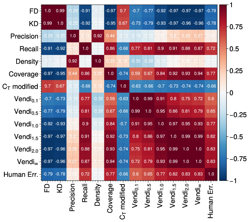
Figure 5: Pearson correlations between metrics averaged across four training datasets. $C_{T}$-modified is computed only on CIFAR-10 and Imagenet256. Vendi scores of large order $q$ correlate strongly with various metrics for evaluating generative models.

We analyze $40$ of the generative models presented in Stein et al. (2023), which spans multiple classes of models and training datasets. In particular, we look at models trained on CIFAR-10  (Krizhevsky et al., 2009), Imagenet256  (Deng et al., 2009), LSUN-Bedroom  (Yu et al., 2015), and FFHQ  (Karras et al., 2019). Further description of the models and metrics is available in the appendix.

Stein et al. (2023) find that the DINOv2 ViT-L/14 network  (Oquab et al., 2023) produces a representation space for which various evaluation metrics align well with human evaluation. We thus use the same network to produce embeddings of the generated outputs from each model. Vendi Scores are computed on these embeddings using a linear kernel.

In Figure 4, we see that Vendi Score_∞ correlates quite well with a model’s ability to produce high-quality images (its Human Error Rate), and $C_{T}$-modified, a memorization metric presented in Stein et al. (2023) that is a modified version of the original $C_{T}$ metric proposed by Meehan et al. (2020). $C_{T}$-modified measures how often a generated data point is closer to the training data than the test data, penalizing models that are closer to the training data. Vendi Score_∞ is most sensitive to large groups of similar samples, likely duplicates. The strong negative correlation between Vendi Score_∞ and $C_{T}$-modified therefore suggests that the models with the highest Vendi Score_∞ are producing large groups of samples around the training data. This also explains why the models with the highest Vendi Score_∞ have high Human Error Rates as well: the samples being produced by the models contain many duplicates that are highly similar to the training data, which will make much of the generated output difficult to classify as fake.

Figure 5 provides a comprehensive overview of all tested metrics and their correlations. Notable in the figure is the strong negative correlation between Vendi Score_∞ and the metrics used to measure sample quality, namely Fréchet Distance (FD)  (Heusel et al., 2017; Stein et al., 2023), and Kernel Distance (KD)  (Bińkowski et al., 2018; Stein et al., 2023). Models with low FD and KD have high sample quality by definition. Due to the strong negative correlation between Vendi Score_∞ and FD and KD, models with good sample quality as measured by FD and KD tend to produce duplicates, since they have high Vendi Score_∞. This is the same conclusion we drew earlier, looking at human error rate and Vendi Score_∞. We also take note of the correlation between the Vendi scores and coverage, another metric used to measure diversity  (Naeem et al., 2020). Coverage measures how many training data points are ’close’ to any generated data point. Models with a high Vendi Score_∞ are producing images centered around the training data, which would satisfy the coverage requirement for those training samples.

6 Discussion

We introduced a family of diversity metrics called Vendi scores that extend the Hill numbers to account for similarity. Unlike the Hill numbers, the Vendi scores are unsupervised in that they don’t require defining a notion of classes, nor do they require knowledge of class prevalence. These scores vary in their overall behavior, such as their sensitivity to imbalanced classes and inter-class variance. Our molecular simulations of Alanine Dipeptide revealed that using a score of order $q=\infty$ actually enables faster mixing, suggesting that the associated eigenvector is aligned with a useful bias potential. We also demonstrated the utility of using the Vendi scores, especially the score of order $q=\infty$, in evaluating image generative models. Our experiments revealed that image generative models that tend to score well on sample quality metrics, e.g. human error rate or Fréchet Distance, are those models that produce duplicates around memorized training samples. This calls for the need to pair sample quality metrics with the Vendi scores, so as to better distinguish models that have high sample quality only because of memorization and duplication around memorized samples and models that do produce sharp samples without memorization.

Limitations.  This paper addressed the limitation of the Vendi Score ($q=1$) under imbalanced settings. A pending problem is the choice of the kernel, which also affects the behavior of the Vendi scores. In future work, we aim to understand how the choice of kernel interfaces with the order $q$. The Vendi scores can also be computationally costly to compute when faced with large collections of data that do not have vector representations. Finding methods for scaling the scores remains an open problem.

Acknowledgements

Adji Bousso Dieng acknowledges support from the National Science Foundation, Office of Advanced Cyberinfrastructure (OAC) #2118201, and from the Schmidt Futures AI2050 Early Career Fellowship. Amey Pasarkar is supported by an NSF-GRFP fellowship. We thank Dan Friedman for insightful discussions.

7 Appendix

7.1 Proof of Theorem 4.1

Theorem 7.1 (The Similarity-Eigenvalue-Prevalence Theorem).

Let $({\mathbf{x}}_{1},\dots,{\mathbf{x}}_{N})$ denote a collection of elements, where each ${\mathbf{x}}_{i}=({\mathbf{x}}_{i1},\dots,{\mathbf{x}}_{iM_{i}})$ contains a unique element repeated $M_{i}$ times, i.e. ${\mathbf{x}}_{ij}={\mathbf{x}}_{ik}$ for all $j,k\in\left\{1,\dots,M_{i}\right\}$. Define $C=\sum_{i=1}^{N}M_{i}$. Let ${\mathbf{K}}\in\mathbb{R}^{C\times C}$ denote a kernel matrix such that ${\mathbf{K}}({\mathbf{x}}_{i\bullet},{\mathbf{x}}_{j\bullet})=1$ when $i=j$ and $0$ otherwise, $\forall i,j\in\left\{1,\dots,N\right\}$. Denote by $\tilde{{\mathbf{K}}}=\frac{{\mathbf{K}}}{C}$ the normalized kernel. Then $\tilde{{\mathbf{K}}}$ has exactly $N$ non-zero eigenvalues $\lambda_{1},\dots,\lambda_{N}$ and $\lambda_{i}=\frac{M_{i}}{C}$ $\forall i\in\left\{1,\dots,N\right\}$.

Proof.

Without loss of generality we construct $\tilde{{\mathbf{K}}}$ as a block diagonal matrix with $N$ blocks, where each block corresponds to a matrix indexed by the elements of ${\mathbf{x}}_{i}$. Denote by ${\mathbf{J}}_{i}$ the $i^{\text{th}}$ block. On the one hand, we have

$$\text{det}(\tilde{{\mathbf{K}}}) =\prod_{i=1}^{N}\text{det}({\mathbf{J}}_{i})\quad\text{and}\quad\text{det}(\tilde{{\mathbf{K}}}-\gamma{\mathbf{I}}_{C})=\prod_{i=1}^{N}\text{det}({\mathbf{J}}_{i}-\gamma{\mathbf{I}}_{M_{i}})$$

for any $\gamma$. Therefore the eigenvalues of $\tilde{{\mathbf{K}}}$ are exactly the collection of the eigenvalues of ${\mathbf{J}}_{1},\dots,{\mathbf{J}}_{N}$. On the other hand, each ${\mathbf{J}}_{i}$ is of size $M_{i}\times M_{i}$ and we have ${\mathbf{J}}_{i}=\frac{1}{C}\left(1\dots 1\right)^{T}\left(1\dots 1\right)$. Therefore rank(${\mathbf{J}}_{i}$) $=1$ and the null space of ${\mathbf{J}}_{i}$ is of dimension $M_{i}-1$. This means ${\mathbf{J}}_{i}$ has $M_{i}-1$ zero eigenvalues. Denote by $\lambda_{i}$ the remaining eigenvalue and by ${\mathbf{v}}_{i}$ its associated eigenvector. We have

$${\mathbf{J}}_{i}({\mathbf{v}}_{i1}\dots\mathbf{v}_{iM_{i}})^{T} =\lambda_{i}({\mathbf{v}}_{i1}\dots\mathbf{v}_{iM_{i}})^{T}$$

$$\frac{1}{C}\left(1\dots 1\right)^{T}\left(1\dots 1\right)({\mathbf{v}}_{i1}\dots\mathbf{v}_{iM_{i}})^{T} =\lambda_{i}({\mathbf{v}}_{i1}\dots\mathbf{v}_{iM_{i}})^{T}$$

$$\frac{1}{C}\left(1\dots 1\right)^{T}\left({\mathbf{v}}_{i1}+\dots+{\mathbf{v}}_{iM_{i}}\right) =\lambda_{i}({\mathbf{v}}_{i1}\dots\mathbf{v}_{iM_{i}})^{T}$$

Then ${\mathbf{v}}_{i}=\left(1\dots 1\right)$ and $\lambda_{i}=\frac{M_{i}}{C}$. Since the eigenvalues of $\tilde{{\mathbf{K}}}$ correspond to the eigenvalues of ${\mathbf{J}}_{1},\dots,{\mathbf{J}}_{N}$, we conclude $\tilde{{\mathbf{K}}}$ has exactly $N$ nonzero eigenvalues $\lambda_{1},\dots,\lambda_{N}$ and $\lambda_{i}=\frac{M_{i}}{C}$ $\forall i$. ∎

7.2 Vendi Sampling: Double Well System

We additionally study the two-dimensional Double Well system from Noé et al. (2019), which is characterized by two imbalanced modes separated by a large energy barrier that standard Langevin dynamics is slow to traverse. Through the addition of the Vendi force, we expect to see fast convergence as well as transitions across this barrier. We perform this set of experiments following the setup used in  Pasarkar et al. (2023).

To compute the Vendi Score, we used the kernel $k(x,x^{\prime})=1-\frac{|x-x^{\prime}|}{|x|+|x^{\prime}|}$. We also use a linear annealing schedule for $\nu$, decreasing it at a constant rate to $0$ for a specified period of time. For each choice of Vendi Score, we determined the optimal hyperparameters using a grid search. In Figure 6, we used the following hyperparameters: For $q=0.1$ and $q=\infty$, we used $\nu=50$ with annealing rate $\frac{1}{50000}$. For $q=0.5$ and $q=1.$, we use $\nu=100$ with annealing rate $\frac{1}{100000}$. And finally for $q=1.5$ and $q=2.$, we used $\nu=50$ with annealing rate $\frac{1}{25000}$. $16$ particles are initialized with random positions sampled from $U[-2.5,2.5]^{2}$ and simulations are performed with a step-size of $10^{-2}$ for $2,000,000$ million steps. We measure convergence using the Free energy difference between the regions $\left\{x\in[-2.5,0],y\in[-4,4]\right\}$ and $\left\{x\in[0,2.5],y\in[-4,4]\right\}$.

We observe that the choice of Vendi Score does not noticeably affect convergence in this system, but that the Vendi Score regularization is indeed quite different across scores. Over the first $100,000$ steps, we find that for Vendi Scores with extreme Hill Numbers, $q=0.1$ and $q=\infty$, there is still a slow transition rate for particles across the boundary while the Vendi force is active compared to other choices of $q$. The slow transition rate is supported by the small Vendi force magnitudes for $q=0.1$ and $q=\infty$.

We have observed that $q=0.1$ leads to a very sensitive Vendi Score, whereas $q=\infty$ gives the least sensitive Vendi Score. Yet, they provide similar effects in the Double Well setting: for $q=0.1$, samples are likely to already be considered diverse and therefore there is not much optimization necessary through the Vendi force. For large $q$, the score is determined only by the largest eigenvalue of the gram matrix $K/n$. Optimizing for the largest eigenvalue may not be informative in some systems.

Meanwhile, for $q=0.5$ and $q=1.0$, the effect of the Vendi Force is largest, demonstrating a trade-off between the sensitivity of small and large Hill Numbers.

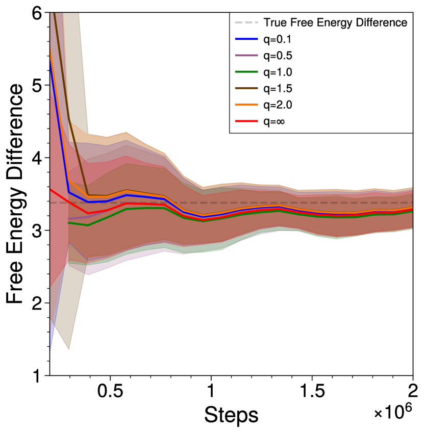
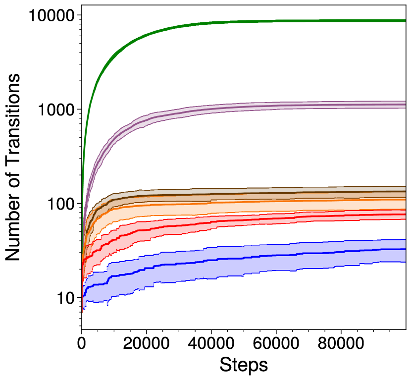
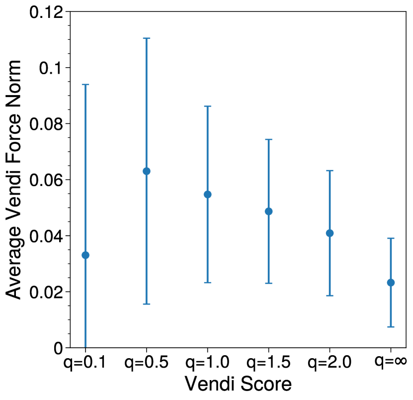
Figure 6: Performance of Different Vendi Scores in Sampling from Double Well Left: Free energy difference over time for each choice of Vendi Score shows similar levels of convergence to the true free energy difference. Hyperparameters are tuned individually for each Vendi Score. Center: Number of transitions of replicas across boundary of $x=0$ over time for each choice of Vendi Score. Hill Numbers farther from $1$ seem to provide less transitions, likely due to smaller gradients, as shown in Right.

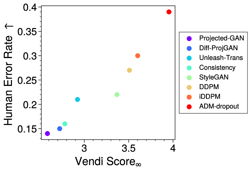
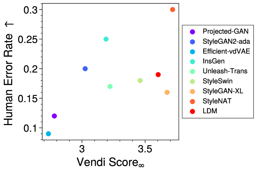
Figure 7: Vendi Score_∞ is well-correlated with human evaluation on LSUN-Bedroom (Left) and FFHQ (Right) datasets.

7.3 Image Generative Model Analysis

Stein et al. (2023) provided analysis of dozens of image generative models across datasets and model types. We study all models for which they provided publically available image outputs. For details regarding dataset curation and model training, we refer the reader to Stein et al. (2023).

For CIFAR-10, there were $6$ StudioGAN models used (Kang et al., 2023a): ACGAN (Odena et al., 2017), BigGAN (Brock et al., 2018), LOGAN (Wu et al., 2019), ReACGAN (Kang et al., 2021), MHGAN (Turner et al., 2019), and WGAN-GP (Gulrajani et al., 2017). Other models tested included LSGM-ODE (Vahdat et al., 2021), iDDPM-DDIM (Nichol and Dhariwal, 2021), PFGM++ (Xu et al., 2023), RESFLOW (Chen et al., 2019), NVAE (Vahdat and Kautz, 2020), StyleGAN2-ada (Karras et al., 2020), StyleGAN2-XL (Sauer et al., 2022).

For Imagenet, we analyzed results from the following models: ADM, ADMG, ADMG-ADMU (Dhariwal and Nichol, 2021), BigGAN (Brock et al., 2018), DiT-XL-2, GigaGAN (Kang et al., 2023b), LDM (Rombach et al., 2022), Mask-GIT (Chang et al., 2022a), RQ-Transformer (Lee et al., 2022), and StyleGAN-XL (Sauer et al., 2022).

For FFHQ, we used the following models: Efficient-vdVAE (Hazami et al., 2022), Insgen (Yang et al., 2021), LDM (Rombach et al., 2022), Projected-GAN (Sauer et al., 2021), StyleGAN2-ada (Karras et al., 2020), StyleGAN2-XL (Sauer et al., 2022), StyleNAT (Walton et al., 2022), StyleSwin (Zhang et al., 2022), and Unleashing-Transformers (Bond-Taylor et al., 2022).

Finally, for LSUN-Bedroom, we use the following models: Unleashing-Transformers (Bond-Taylor et al., 2022), Projected-GAN (Sauer et al., 2021), ADMNet-dropout (Dhariwal and Nichol, 2021), DDPM (Ho et al., 2020), iDDPM (Nichol and Dhariwal, 2021), StyleGAN (Karras et al., 2019), Diffusion-projected GAN (Wang et al., 2022), and Consistency (Meehan et al., 2020).

We also show that the Human Error Rate is strongly correlated with Vendi Score_∞ on the LSUN-Bedroom and FFHQ datasets in Figure 7.

References

- Benhenda (2017) Benhenda, M. (2017). Chemgan challenge for drug discovery: can ai reproduce natural chemical diversity? arXiv preprint arXiv:1708.08227.
- Berns et al. (2023) Berns, S., Colton, S., and Guckelsberger, C. (2023). Towards mode balancing of generative models via diversity weights. arXiv preprint arXiv:2304.11961.
- Bińkowski et al. (2018) Bińkowski, M., Sutherland, D., Arbel, M., Gretton, A., and Demystifying, M. (2018). Gans. In International Conference on Learning Representations (ICLR).
- Bond-Taylor et al. (2022) Bond-Taylor, S., Hessey, P., Sasaki, H., Breckon, T. P., and Willcocks, C. G. (2022). Unleashing transformers: Parallel token prediction with discrete absorbing diffusion for fast high-resolution image generation from vector-quantized codes. In European Conference on Computer Vision, pages 170–188. Springer.
- Brock et al. (2018) Brock, A., Donahue, J., and Simonyan, K. (2018). Large scale gan training for high fidelity natural image synthesis. arXiv preprint arXiv:1809.11096.
- Chang et al. (2022a) Chang, H., Zhang, H., Jiang, L., Liu, C., and Freeman, W. T. (2022a). Maskgit: Masked generative image transformer. In Proceedings of the IEEE/CVF Conference on Computer Vision and Pattern Recognition, pages 11315–11325.
- Chang et al. (2022b) Chang, L., Perez, A., and Miranda-Quintana, R. A. (2022b). Improving the analysis of biological ensembles through extended similarity measures. Physical Chemistry Chemical Physics, 24(1):444–451.
- Chen et al. (2019) Chen, R. T., Behrmann, J., Duvenaud, D. K., and Jacobsen, J.-H. (2019). Residual flows for invertible generative modeling. Advances in Neural Information Processing Systems, 32.
- Deng et al. (2009) Deng, J., Dong, W., Socher, R., Li, L.-J., Li, K., and Fei-Fei, L. (2009). Imagenet: A large-scale hierarchical image database. In 2009 IEEE conference on computer vision and pattern recognition, pages 248–255. Ieee.
- Dhariwal and Nichol (2021) Dhariwal, P. and Nichol, A. (2021). Diffusion models beat gans on image synthesis. Advances in neural information processing systems, 34:8780–8794.
- Diamantis et al. (2023) Diamantis, D. E., Gatoula, P., Koulaouzidis, A., and Iakovidis, D. K. (2023). This intestine does not exist: Multiscale residual variational autoencoder for realistic wireless capsule endoscopy image generation. arXiv preprint arXiv:2302.02150.
- Dieng et al. (2019) Dieng, A. B., Ruiz, F. J., Blei, D. M., and Titsias, M. K. (2019). Prescribed generative adversarial networks. arXiv preprint arXiv:1910.04302.
- Eastman et al. (2017) Eastman, P., Swails, J., Chodera, J. D., McGibbon, R. T., Zhao, Y., Beauchamp, K. A., Wang, L.-P., Simmonett, A. C., Harrigan, M. P., Stern, C. D., et al. (2017). Openmm 7: Rapid development of high performance algorithms for molecular dynamics. PLoS computational biology, 13(7):e1005659.
- Eysenbach et al. (2018) Eysenbach, B., Gupta, A., Ibarz, J., and Levine, S. (2018). Diversity is all you need: Learning skills without a reward function. arXiv preprint arXiv:1802.06070.
- Fomicheva et al. (2020) Fomicheva, M., Sun, S., Yankovskaya, L., Blain, F., Guzmán, F., Fishel, M., Aletras, N., Chaudhary, V., and Specia, L. (2020). Unsupervised quality estimation for neural machine translation. Transactions of the Association for Computational Linguistics, 8:539–555.
- Friedman and Dieng (2022) Friedman, D. and Dieng, A. B. (2022). The vendi score: A diversity evaluation metric for machine learning. arXiv preprint arXiv:2210.02410.
- Gulrajani et al. (2017) Gulrajani, I., Ahmed, F., Arjovsky, M., Dumoulin, V., and Courville, A. C. (2017). Improved training of wasserstein gans. Advances in neural information processing systems, 30.
- Hazami et al. (2022) Hazami, L., Mama, R., and Thurairatnam, R. (2022). Efficientvdvae: Less is more. arXiv preprint arXiv:2203.13751.
- Heusel et al. (2017) Heusel, M., Ramsauer, H., Unterthiner, T., Nessler, B., and Hochreiter, S. (2017). Gans trained by a two time-scale update rule converge to a local nash equilibrium. Advances in neural information processing systems, 30.
- Hill (1973) Hill, M. O. (1973). Diversity and evenness: a unifying notation and its consequences. Ecology, 54(2):427–432.
- Ho et al. (2020) Ho, J., Jain, A., and Abbeel, P. (2020). Denoising diffusion probabilistic models. Advances in neural information processing systems, 33:6840–6851.
- Jaini et al. (2021) Jaini, P., Holdijk, L., and Welling, M. (2021). Learning equivariant energy based models with equivariant stein variational gradient descent. Advances in Neural Information Processing Systems, 34:16727–16737.
- Kang et al. (2021) Kang, M., Shim, W., Cho, M., and Park, J. (2021). Rebooting acgan: Auxiliary classifier gans with stable training. Advances in neural information processing systems, 34:23505–23518.
- Kang et al. (2023a) Kang, M., Shin, J., and Park, J. (2023a). Studiogan: a taxonomy and benchmark of gans for image synthesis. IEEE Transactions on Pattern Analysis and Machine Intelligence.
- Kang et al. (2023b) Kang, M., Zhu, J.-Y., Zhang, R., Park, J., Shechtman, E., Paris, S., and Park, T. (2023b). Scaling up gans for text-to-image synthesis. In Proceedings of the IEEE/CVF Conference on Computer Vision and Pattern Recognition, pages 10124–10134.
- Karras et al. (2020) Karras, T., Aittala, M., Hellsten, J., Laine, S., Lehtinen, J., and Aila, T. (2020). Training generative adversarial networks with limited data. In Proc. NeurIPS.
- Karras et al. (2019) Karras, T., Laine, S., and Aila, T. (2019). A style-based generator architecture for generative adversarial networks. In Proceedings of the IEEE/CVF conference on computer vision and pattern recognition, pages 4401–4410.
- Krizhevsky et al. (2009) Krizhevsky, A., Hinton, G., et al. (2009). Learning multiple layers of features from tiny images.
- Lee et al. (2022) Lee, D., Kim, C., Kim, S., Cho, M., and Han, W.-S. (2022). Autoregressive image generation using residual quantization. In Proceedings of the IEEE/CVF Conference on Computer Vision and Pattern Recognition, pages 11523–11532.
- Leinster (2020) Leinster, T. (2020). Entropy and diversity: The axiomatic approach. arXiv preprint arXiv:2012.02113.
- Leinster and Cobbold (2012) Leinster, T. and Cobbold, C. A. (2012). Measuring diversity: the importance of species similarity. Ecology, 93(3):477–489.
- Maus et al. (2022) Maus, N., Wu, K., Eriksson, D., and Gardner, J. (2022). Discovering many diverse solutions with bayesian optimization. arXiv preprint arXiv:2210.10953.
- Meehan et al. (2020) Meehan, C., Chaudhuri, K., and Dasgupta, S. (2020). A non-parametric test to detect data-copying in generative models. In International Conference on Artificial Intelligence and Statistics.
- Miranda-Quintana et al. (2021) Miranda-Quintana, R. A., Rácz, A., Bajusz, D., and Héberger, K. (2021). Extended similarity indices: the benefits of comparing more than two objects simultaneously. part 2: speed, consistency, diversity selection. Journal of Cheminformatics, 13(1):33.
- Mouret and Clune (2015) Mouret, J.-B. and Clune, J. (2015). Illuminating search spaces by mapping elites. arXiv preprint arXiv:1504.04909.
- Naeem et al. (2020) Naeem, M. F., Oh, S. J., Uh, Y., Choi, Y., and Yoo, J. (2020). Reliable fidelity and diversity metrics for generative models. In International Conference on Machine Learning, pages 7176–7185. PMLR.
- Nguyen and Garnett (2023) Nguyen, Q. and Garnett, R. (2023). Nonmyopic multiclass active search with diminishing returns for diverse discovery. In International Conference on Artificial Intelligence and Statistics, pages 5231–5249. PMLR.
- Nichol and Dhariwal (2021) Nichol, A. Q. and Dhariwal, P. (2021). Improved denoising diffusion probabilistic models. In International Conference on Machine Learning, pages 8162–8171. PMLR.
- Noé et al. (2019) Noé, F., Olsson, S., Köhler, J., and Wu, H. (2019). Boltzmann generators: Sampling equilibrium states of many-body systems with deep learning. Science, 365(6457):eaaw1147.
- Odena et al. (2017) Odena, A., Olah, C., and Shlens, J. (2017). Conditional image synthesis with auxiliary classifier gans. In International conference on machine learning, pages 2642–2651. PMLR.
- Oquab et al. (2023) Oquab, M., Darcet, T., Moutakanni, T., Vo, H., Szafraniec, M., Khalidov, V., Fernandez, P., Haziza, D., Massa, F., El-Nouby, A., et al. (2023). Dinov2: Learning robust visual features without supervision. arXiv preprint arXiv:2304.07193.
- Pasarkar et al. (2023) Pasarkar, A. P., Bencomo, G. M., Olsson, S., and Dieng, A. B. (2023). Vendi sampling for molecular simulations: Diversity as a force for faster convergence and better exploration. The Journal of Chemical Physics, 159(14).
- Pugh et al. (2016) Pugh, J. K., Soros, L. B., and Stanley, K. O. (2016). Quality diversity: A new frontier for evolutionary computation. Frontiers in Robotics and AI, 3:40.
- Rácz et al. (2022) Rácz, A., Mihalovits, L. M., Bajusz, D., Héberger, K., and Miranda-Quintana, R. A. (2022). Molecular dynamics simulations and diversity selection by extended continuous similarity indices. Journal of Chemical Information and Modeling, 62(14):3415–3425.
- Rombach et al. (2022) Rombach, R., Blattmann, A., Lorenz, D., Esser, P., and Ommer, B. (2022). High-resolution image synthesis with latent diffusion models. In Proceedings of the IEEE/CVF conference on computer vision and pattern recognition, pages 10684–10695.
- Sajjadi et al. (2018) Sajjadi, M. S., Bachem, O., Lucic, M., Bousquet, O., and Gelly, S. (2018). Assessing generative models via precision and recall. Advances in neural information processing systems, 31.
- Sauer et al. (2021) Sauer, A., Chitta, K., Müller, J., and Geiger, A. (2021). Projected gans converge faster. Advances in Neural Information Processing Systems, 34:17480–17492.
- Sauer et al. (2022) Sauer, A., Schwarz, K., and Geiger, A. (2022). Stylegan-xl: Scaling stylegan to large diverse datasets. In ACM SIGGRAPH 2022 conference proceedings, pages 1–10.
- Shen et al. (2019) Shen, T., Ott, M., Auli, M., and Ranzato, M. (2019). Mixture models for diverse machine translation: Tricks of the trade. In International conference on machine learning, pages 5719–5728. PMLR.
- Stein et al. (2023) Stein, G., Cresswell, J. C., Hosseinzadeh, R., Sui, Y., Ross, B. L., Villecroze, V., Liu, Z., Caterini, A. L., Taylor, J. E. T., and Loaiza-Ganem, G. (2023). Exposing flaws of generative model evaluation metrics and their unfair treatment of diffusion models. arXiv preprint arXiv:2306.04675.
- Turner et al. (2019) Turner, R., Hung, J., Frank, E., Saatchi, Y., and Yosinski, J. (2019). Metropolis-hastings generative adversarial networks. In International Conference on Machine Learning, pages 6345–6353. PMLR.
- Vahdat and Kautz (2020) Vahdat, A. and Kautz, J. (2020). Nvae: A deep hierarchical variational autoencoder. Advances in neural information processing systems, 33:19667–19679.
- Vahdat et al. (2021) Vahdat, A., Kreis, K., and Kautz, J. (2021). Score-based generative modeling in latent space. Advances in Neural Information Processing Systems, 34:11287–11302.
- Vassiliades et al. (2017) Vassiliades, V., Chatzilygeroudis, K., and Mouret, J.-B. (2017). Using centroidal voronoi tessellations to scale up the multidimensional archive of phenotypic elites algorithm. IEEE Transactions on Evolutionary Computation, 22(4):623–630.
- Walton et al. (2022) Walton, S., Hassani, A., Xu, X., Wang, Z., and Shi, H. (2022). Stylenat: Giving each head a new perspective. arXiv preprint arXiv:2211.05770.
- Wang et al. (2022) Wang, Z., Zheng, H., He, P., Chen, W., and Zhou, M. (2022). Diffusion-gan: Training gans with diffusion. arXiv preprint arXiv:2206.02262.
- Whittaker (1972) Whittaker, R. H. (1972). Evolution and measurement of species diversity. Taxon, 21(2-3):213–251.
- Wu et al. (2019) Wu, Y., Donahue, J., Balduzzi, D., Simonyan, K., and Lillicrap, T. (2019). Logan: Latent optimisation for generative adversarial networks. arXiv preprint arXiv:1912.00953.
- Xu et al. (2023) Xu, Y., Liu, Z., Tian, Y., Tong, S., Tegmark, M., and Jaakkola, T. (2023). Pfgm++: Unlocking the potential of physics-inspired generative models. arXiv preprint arXiv:2302.04265.
- Yang et al. (2021) Yang, C., Shen, Y., Xu, Y., and Zhou, B. (2021). Data-efficient instance generation from instance discrimination. Advances in Neural Information Processing Systems, 34:9378–9390.
- Yu et al. (2015) Yu, F., Seff, A., Zhang, Y., Song, S., Funkhouser, T., and Xiao, J. (2015). Lsun: Construction of a large-scale image dataset using deep learning with humans in the loop. arXiv preprint arXiv:1506.03365.
- Zhang et al. (2022) Zhang, B., Gu, S., Zhang, B., Bao, J., Chen, D., Wen, F., Wang, Y., and Guo, B. (2022). Styleswin: Transformer-based gan for high-resolution image generation. In Proceedings of the IEEE/CVF conference on computer vision and pattern recognition, pages 11304–11314.