Abstract

The recently proposed generative flow networks (GFlowNets) are a method of training a policy to sample compositional discrete objects with probabilities proportional to a given reward via a sequence of actions. GFlowNets exploit the sequential nature of the problem, drawing parallels with reinforcement learning (RL). Our work extends the connection between RL and GFlowNets to a general case. We demonstrate how the task of learning a generative flow network can be efficiently redefined as an entropy-regularized RL problem with a specific reward and regularizer structure. Furthermore, we illustrate the practical efficiency of this reformulation by applying standard soft RL algorithms to GFlowNet training across several probabilistic modeling tasks. Contrary to previously reported results, we show that entropic RL approaches can be competitive against established GFlowNet training methods. This perspective opens a direct path for integrating reinforcement learning principles into the realm of generative flow networks.

1 INTRODUCTION

Generative flow networks (GFlowNet, Bengio et al.,, 2021) are models designed to learn a sampler from a complex discrete space according to a probability mass function given up to an unknown normalizing constant. A fundamental assumption underlying GFlowNets is an additional sequential structure of the space: any object can be generated by following a sequence of actions starting from an initial state, which induces a directed acyclic graph over "incomplete" objects. In essence, GFlowNet aims to learn a stochastic policy to select actions and navigate in this graph in order to match a distribution over final objects with the desired one. A motivational example of the work Bengio et al., (2021) was molecule generation: GFlowNet starts from an empty molecule and learns a policy that adds various blocks sequentially in order to match a desired distribution over a certain molecule space.

The problem statement shares a lot of similarity with reinforcement learning (RL, Sutton and Barto,, 2018) and indeed existing generative flow network algorithms often borrow ideas from RL. In particular, the original GFlowNet training method called flow matching (Bengio et al.,, 2021) was inspired by temporal-difference learning (Sutton,, 1988). Next, established techniques in RL were a large source of inspiration for developing novel GFlowNet techniques: subtrajectory balance loss (Madan et al.,, 2023) was inspired by $\mathrm{TD}(\lambda)$; a prioritized experience replay idea (Lin,, 1992; Schaul et al.,, 2016) was actively used in (Shen et al.,, 2023; Vemgal et al.,, 2023); distributional perspective on RL (Bellemare et al.,, 2023) also appears in GFlowNet literature (Zhang et al.,, 2023). Additionally, various RL exploration techniques (Osband et al.,, 2016; Ostrovski et al.,, 2017; Burda et al.,, 2019) also were recently adapted into the GFlowNet framework (Pan et al.,, 2023; Rector-Brooks et al.,, 2023).

This large source of techniques results in a question about a more rigorous connection between RL and GFlowNets. Unfortunately, RL problem with the classic goal of return maximization solely cannot adequately address the sampling problem since the final optimal policies are deterministic or close to deterministic. However, there exists a paradigm of entropy regularized RL (Fox et al.,, 2016; Haarnoja et al.,, 2017; Schulman et al., 2017a, ) (also known as MaxEnt RL and soft RL), where a final goal is to find a policy that will not only maximize return but also be close to a uniform one, resulting in energy-based representation of the optimal policies (Haarnoja et al.,, 2017).

The authors of Bengio et al., (2021) have drawn a direct connection between MaxEnt RL and GFlowNets in the setup of auto-regressive generation, or, equivalently, in the setting where the corresponding generation graph is a tree. However, the presented reduction does not hold in the setting of general graphs and results in a generation from a highly biased distribution. After that, the authors of Bengio et al., (2023) concluded that the direct connection holds only in the tree setup.

In our work, we refute this claim and show that it is possible to reduce the GFlowNet learning problem to entropy-regularized RL beyond the setup of tree-structured graphs.

The main corollary of our result is the possibility to directly apply existing RL techniques without the need to additionally adapt them within GFlowNet framework.

We highlight our main contributions:

• We establish a connection between a GFlowNet problem and entropy regularized RL by a direct reduction;

• We represent detailed balance (Bengio et al.,, 2023) and trajectory balance (Malkin et al.,, 2022) algorithms as existing soft RL algorithms;

• We show how to apply the proposed reduction practically by transmitting SoftDQN (Haarnoja et al.,, 2017) and MunchausenDQN (Vieillard et al., 2020b, ) into the realm of GFlowNets;

• Finally, we provide experimental validation of our theoretical results and show that MaxEnt RL algorithms can be competitive or even outperform established GFlowNet training methods, contrary to previously reported results (Bengio et al.,, 2021).

Source code: github.com/d-tiapkin/gflownet-rl.

2 BACKGROUND

2.1 Generative Flow Networks

In this section we provide some essential definitions and background on GFlowNets. All proofs of the following statements can be found in Bengio et al., (2021) and Bengio et al., (2023).

Suppose we have a finite discrete space of objects $\mathcal{X}$ with a black-box non-negative reward function $\mathcal{R}(x)$ given for every $x\in\mathcal{X}$. Our goal is to construct and train a model that will sample objects from $\mathcal{X}$ from the probability distribution $\mathcal{R}(x)/\mathrm{Z}$ proportional to the reward, where $\mathrm{Z}$ is an unknown normalizing constant.

Flows over Directed Acyclic Graphs

The generation process in GFlowNets is viewed as a sequence of constructive actions where we start with an "empty" object and at each step add some new component to it. To formally describe this process, a finite direct acyclic graph (DAG) $\mathcal{G}=(\mathcal{S},\mathcal{E})$ is introduced, where $\mathcal{S}$ is a state space and $\mathcal{E}\subseteq\mathcal{S}\times\mathcal{S}$ is a set of edges. For each state $s\in\mathcal{S}$ we define a set of actions $\mathcal{A}_{s}$ as possible next states: $s^{\prime}\in\mathcal{A}_{s}\Leftrightarrow s\to s^{\prime}\in\mathcal{E}$. The action corresponds to adding some new component to the object, transforming an object $s$ into a new object $s^{\prime}$. If $s^{\prime}\in\mathcal{A}_{s}$ we say that $s^{\prime}$ is a child of $s$ and $s$ is a parent of $s^{\prime}$. There is a special initial state $s_{0}\in\mathcal{S}$ associated with an "empty" object, and it is the only state that has no incoming edges. All other states can be reached from $s_{0}$, and the set of terminal states (states with no outgoing edges) directly corresponds to the initial space of interest $\mathcal{X}$.

Denote $\mathcal{T}$ as a set of all complete trajectories in the graph $\tau=\mathopen{}\mathclose{{}\left(s_{0}\to s_{1}\to\ldots\to s_{n_{\tau}}}\right)$, where $n_{\tau}$ is the trajectory length, $s_{i}\to s_{i+1}\in\mathcal{E}$, $s_{0}$ is always the initial state, and $s_{n_{\tau}}$ is always a terminal state, thus $s_{n_{\tau}}\in\mathcal{X}$. As a result, any complete trajectory can be viewed as a sequence of actions that constructs the object corresponding to $s_{n_{\tau}}$ staring from $s_{0}$. A trajectory flow is any nonnegative function $\mathcal{F}\colon\mathcal{T}\to\mathbb{R}_{\geq 0}$. If $\mathcal{F}$ is not identically zero, it can be used to introduce a probability distribution over complete trajectories:

$$\mathcal{P}(\tau)\triangleq\frac{1}{\mathrm{Z}_{\mathcal{F}}}\mathcal{F}(\tau),\quad\rm\mathrm{Z}_{\mathcal{F}}\triangleq\sum_{\tau\in\mathcal{T}}\mathcal{F}(\tau).$$

After that, flows for states and edges are introduced as

$$\mathcal{F}(s)\triangleq\sum_{\tau\ni s}\mathcal{F}(\tau),\quad\mathcal{F}\mathopen{}\mathclose{{}\left(s\to s^{\prime}}\right)\triangleq\sum_{\tau\ni(s\to s^{\prime})}\mathcal{F}(\tau).$$

Then, $\mathcal{F}(s)/\rm\mathrm{Z}_{\mathcal{F}}$ corresponds to the probability that a random trajectory contains the state $s$, and $\mathcal{F}(s\to s^{\prime})/\rm\mathrm{Z}_{\mathcal{F}}$ corresponds to the probability that a random trajectory contains the edge $s\to s^{\prime}$. These definitions also imply $\mathrm{Z}_{\mathcal{F}}=\mathcal{F}(s_{0})=\sum_{x\in\mathcal{X}}\mathcal{F}(x)$.

Denote $\mathcal{P}(x)$ as the probability that $x$ is the terminal state of a trajectory sampled from $\mathcal{P}(\tau)$. If the reward matching constraint is satisfied for all terminal states $x\in\mathcal{X}$:

$$\mathcal{F}(x)=\mathcal{R}(x),$$ (1)

$\mathcal{P}(x)$ will be equal to $\mathcal{R}(x)/\mathrm{Z}$. Thus by sampling trajectories we can sample the objects from the distribution of interest.

Markovian Flows

To allow efficient sampling of trajectories, the family of trajectory flows considered in practice is narrowed down to Markovian flows. The trajectory flow $\mathcal{F}$ is said to be Markovian if $\forall s\in\mathcal{S}\setminus\mathcal{X}$ there exist distributions $\mathcal{P}_{\mathrm{F}}(-|s)$ over the children of $s$ such that $\mathcal{P}$ can be factorized as

$$\mathcal{P}\mathopen{}\mathclose{{}\left(\tau=\mathopen{}\mathclose{{}\left(s_{0}\rightarrow\ldots\rightarrow s_{n_{\tau}}}\right)}\right)=\prod_{t=1}^{n_{\tau}}\mathcal{P}_{\mathrm{F}}\mathopen{}\mathclose{{}\left(s_{t}|s_{t-1}}\right).$$

This means that trajectories can be sampled by iteratively sampling next states from $\mathcal{P}_{\mathrm{F}}(-\mid s_{i})$ (sequential construction of the object). Equivalently, $\mathcal{F}$ is Markovian if $\forall s\in\mathcal{S}\setminus\{s_{0}\}$ there exist distributions $\mathcal{P}_{\mathrm{B}}(-|s)$ over the parents of $s$ such that $\forall x\in\mathcal{X}$

$$\mathcal{P}\mathopen{}\mathclose{{}\left(\tau=\mathopen{}\mathclose{{}\left(s_{0}\rightarrow\ldots\rightarrow s_{n_{\tau}}}\right)|s_{n_{\tau}}=x}\right)=\prod_{t=1}^{n_{\tau}}\mathcal{P}_{\mathrm{B}}\mathopen{}\mathclose{{}\left(s_{t-1}|s_{t}}\right),$$

​​which means that trajectories ending at $x$ can be sampled by iteratively sampling previous states from $\mathcal{P}_{\mathrm{B}}(-\mid s_{i})$. If $\mathcal{F}$ is Markovian, then $\mathcal{P}_{\mathrm{F}}$ and $\mathcal{P}_{\mathrm{B}}$ can be uniquely defined as

$$\mathcal{P}_{\mathrm{F}}\mathopen{}\mathclose{{}\left(s^{\prime}|s}\right)=\frac{\mathcal{F}\mathopen{}\mathclose{{}\left(s\rightarrow s^{\prime}}\right)}{\mathcal{F}(s)},\quad\mathcal{P}_{\mathrm{B}}\mathopen{}\mathclose{{}\left(s|s^{\prime}}\right)=\frac{\mathcal{F}\mathopen{}\mathclose{{}\left(s\rightarrow s^{\prime}}\right)}{\mathcal{F}\mathopen{}\mathclose{{}\left(s^{\prime}}\right)}.$$ (2)

We call $\mathcal{P}_{\mathrm{F}}$ and $\mathcal{P}_{\mathrm{B}}$ the forward policy and the backward policy. The detailed balance constraint is a relation between them:

$$\mathcal{F}(s)\mathcal{P}_{\mathrm{F}}(s^{\prime}|s)=\mathcal{F}(s^{\prime})\mathcal{P}_{\mathrm{B}}(s|s^{\prime}).$$ (3)

The trajectory balance constraint states that for any complete trajectory

$$\prod_{t=1}^{n_{\tau}}\mathcal{P}_{\mathrm{F}}\mathopen{}\mathclose{{}\left(s_{t}|s_{t-1}}\right)=\frac{\mathcal{F}(s_{n_{\tau}})}{\mathrm{Z}_{\mathcal{F}}}\prod_{t=1}^{n_{\tau}}\mathcal{P}_{\mathrm{B}}\mathopen{}\mathclose{{}\left(s_{t-1}|s_{t}}\right).$$ (4)

Thus any Markovian flow can be uniquely determined from $Z_{\mathcal{F}}$ and $\mathcal{P}_{\mathrm{F}}(-|s)\;\forall s\in\mathcal{S}\setminus\mathcal{X}$ or from $\mathcal{F}(x)\;\forall x\in\mathcal{X}$ and $\mathcal{P}_{\mathrm{B}}(-|s)\;\forall s\in\mathcal{S}\setminus\{s_{0}\}$.

Training GFlowNets

In essence, GFlowNet is a model that parameterizes Markovian flows over some fixed DAG and is trained to minimize some objective. The objective should be chosen in such a way that, if the model is capable of parameterizing any Markovian flow, global minimization of the objective will lead to producing a flow that satisfies (1). Thus forward policy of a trained GFlowNet can be used as a sampler from the reward distribution. Two of the widely used training objectives are:

Trajectory Balance (TB). Introduced in Malkin et al., (2022), based on trajectory balance constraint (4). A model with parameters $\theta$ predicts the normalizing constant $\mathrm{Z}_{\theta}$, forward policy $\mathcal{P}_{\mathrm{F}}(-|s,\theta)$ and backward policy $\mathcal{P}_{\mathrm{B}}(-|s,\theta)$. The trajectory balance objective is defined for each complete trajectory $\tau=\mathopen{}\mathclose{{}\left(s_{0}\to s_{1}\to\ldots\to s_{n_{\tau}}=x}\right)$:

$$\mathcal{L}_{\mathrm{TB}}(\tau)=\mathopen{}\mathclose{{}\left(\log\frac{\mathrm{Z}_{\theta}\prod_{t=1}^{n_{\tau}}\mathcal{P}_{\mathrm{F}}(s_{t}|s_{t-1},\theta)}{\mathcal{R}(x)\prod_{t=1}^{n_{\tau}}\mathcal{P}_{\mathrm{B}}(s_{t-1}|s_{t},\theta)}}\right)^{2}.$$ (5)

Detailed Balance (DB). Introduced in Bengio et al., (2023), based on detailed balance constraint (3). A model with parameters $\theta$ predicts state flows $\mathcal{F}_{\theta}(s)$, forward policy $\mathcal{P}_{\mathrm{F}}(-|s,\theta)$ and backward policy $\mathcal{P}_{\mathrm{B}}(-|s,\theta)$. It is important to note that such parameterization is excessive and the components are not necessarily compatible with each other during the course of training. The detailed balance objective is defined for each edge $s\to s^{\prime}\in\mathcal{E}$:

$$\mathcal{L}_{\mathrm{DB}}(s,s^{\prime})=\mathopen{}\mathclose{{}\left(\log\frac{\mathcal{F}_{\theta}(s)\mathcal{P}_{\mathrm{F}}(s^{\prime}|s,\theta)}{\mathcal{F}_{\theta}(s^{\prime})\mathcal{P}_{\mathrm{B}}(s|s^{\prime},\theta)}}\right)^{2}.$$ (6)

​​For terminal states $\mathcal{F}_{\theta}(x)$ is substituted by $\mathcal{R}(x)$ in the objective.

During the training, the objective of choice is stochastically optimized across complete trajectories sampled from a training policy (which is usually taken to be $\mathcal{P}_{\mathrm{F}}$, a tempered version of it or a mixture of $\mathcal{P}_{\mathrm{F}}$ and a uniform distribution). An important note is that for all objectives $\mathcal{P}_{\mathrm{B}}(-\mid s)$ can either be trained or fixed, e.g. to be uniform over the parents of $s$. When the backward policy is fixed, the corresponding forward policy is uniquely determined by by $\mathcal{P}_{\mathrm{B}}$ and $\mathcal{R}$.

Among other existing objectives, the originally proposed flow matching objective Bengio et al., (2021) was shown to have worse performance than TB and DB (Malkin et al.,, 2022; Madan et al.,, 2023). Recently, subtrajectory balance (SubTB) (Madan et al.,, 2023) was introduced as a generalization of TB and DB and shown to have better performance when appropriately tuned.

2.2 Soft Reinforcement Learning

In this section we describe the main aspects of usual reinforcement learning and its entropy-regularized version, also known as MaxEnt and Soft RL.

Markov Decision Process

The main theoretical object of RL is Markov decision process (MDP) that is defined as a tuple $\mathcal{M}=(\mathcal{S},\mathcal{A},\mathrm{P},r,\gamma,s_{0})$, where $\mathcal{S}$ and $\mathcal{A}$ are finite state and action space, $\mathrm{P}$ is a Markovian transition kernel, $r$ is a bounded deterministic reward function, $\gamma\in[0,1]$ is a discount factor, and $s_{0}$ is a fixed initial state. Additionally, for each state $s$ we define a set of possible actions as $\mathcal{A}_{s}\subseteq\mathcal{A}$. An RL agent interacts with MDP by a policy $\pi$ that maps each state $s$ to a probability distribution over possible actions.

Entropy-Regularized RL

The performance measure of the agent in a classic RL is a value that is defined as an expected (discounted) sum of rewards over trajectory generated by following a policy $\pi$ starting from a state $s$. In contrast, in entropy-regularized reinforcement learning (Neu et al.,, 2017; Geist et al.,, 2019) the value is augmented by Shannon entropy:

$$\textstyle V^{\pi}_{\lambda}(s)\triangleq\mathbb{E}_{\pi}\mathopen{}\mathclose{{}\left[\sum_{t=0}^{\infty}\gamma^{t}(r(s_{t},a_{t})+\lambda\mathcal{H}(\pi(s_{t})))|s_{0}=s}\right],$$ (7)

where $\lambda$ is a regularization coefficient, $\mathcal{H}$ is a Shannon entropy function, $a_{t}\sim\pi(s_{t}),s_{t+1}\sim\mathrm{P}(s_{t},a_{t})$ for all $t\geq 0$, and expectation is taken with respect to these random variables. In a similar manner we can define regularized Q-values $Q^{\pi}_{\lambda}(s,a)$ as an expected (discounted) sum of rewards augmented by Shannon entropy given fixed initial state $s_{0}=s$ and action $a_{0}=a$. A regularized optimal policy $\pi^{\star}_{\lambda}$ is a policy that maximizes $V^{\pi}_{\lambda}(s)$ for any initial state $s$. In the case $\lambda=1$ we will drop a subscript $\lambda$ for brevity.

Soft Bellman Equations

Let $V^{\star}_{\lambda}$ and $Q^{\star}_{\lambda}$ be a value and Q-value of an optimal policy $\pi^{\star}_{\lambda}$ correspondingly. Then Theorem 1 and 2 by Haarnoja et al., (2017) imply the following system relations for any $s\in\mathcal{S},a\in\mathcal{A}_{s}$

$$\begin{split}Q^{\star}_{\lambda}(s,a)&\triangleq r(s,a)+\gamma\mathbb{E}_{s^{\prime}\sim\mathrm{P}(s,a)}[V^{\star}(s^{\prime})]\\ V^{\star}_{\lambda}(s)&\triangleq\mathrm{LogSumExp}_{\lambda}\mathopen{}\mathclose{{}\left(Q^{\star}_{\lambda}(s,\cdot)}\right),\end{split}$$ (8)

where $\mathrm{LogSumExp}_{\lambda}(x)\triangleq\lambda\log(\sum_{i=1}^{d}{\rm e}^{x_{i}/\lambda})$, and an optimal policy is defined as a $\lambda$-softmax policy with respect to optimal Q-values $\pi^{\star}_{\lambda}(s)=\mathrm{Softmax}_{\lambda}(Q^{\star}_{\lambda}(s,\cdot))$, where $[\mathrm{Softmax}_{\lambda}(x)]_{i}\triangleq{\rm e}^{x_{i}/\lambda}/(\sum_{j=1}^{d}{\rm e}^{x_{j}/\lambda})$, or, alternatively

$$\textstyle\pi^{\star}_{\lambda}(a|s)=\exp\mathopen{}\mathclose{{}\left(\frac{1}{\lambda}\mathopen{}\mathclose{{}\left(Q^{\star}_{\lambda}(s,a)-V^{\star}_{\lambda}(s)}\right)}\right).$$ (9)

Notice that as $\lambda\to 0$ we recover the well-known Bellman equations (see e.g. Sutton and Barto, (2018)) since $\mathrm{LogSumExp}_{\lambda}$ approximates maximum and $\mathrm{Softmax}_{\lambda}$ approximates a uniform distribution over $\operatorname*{arg\,max}$.

Soft Deep Q-Network

One of the classic ways to solve RL problem for discrete control problem is well-known Deep Q-Network algorithm (DQN) (Mnih et al.,, 2015). Next we present the generalization of this will-known algorithm to entropy-regularized RL problems called SoftDQN (also known as SoftQLearning (Fox et al.,, 2016; Haarnoja et al.,, 2017; Schulman et al., 2017a, ) in a continuous control setting).

The goal of SoftDQN algorithm is to approximate a solution to soft Bellman equations (8) using a Q-value parameterized by a neural network. Let $Q_{\theta}$ be an online Q-network, it represents the current approximation of optimal regularized Q-value. Also let $\pi_{\theta}=\mathrm{Softmax}_{\lambda}(Q_{\theta})$ be a policy that approximates the optimal policy. Then, akin to DQN, agent interacts with MDP using policy $\pi_{\theta}$ (with an additional $\varepsilon$-greedy exploration or even without it), collect transitions $(s_{t},a_{t},r_{t},s_{t+1})$ for $r_{t}=r(s_{t},a_{t})$ in a replay buffer $\mathcal{B}$. Then SoftDQN performs stochastic gradient descent on the regression loss $\mathcal{L}_{\texttt{SoftDQN}}(\mathcal{B})=\mathbb{E}_{\mathcal{B}}[(Q_{\theta}(s_{t},a_{t})-y_{\texttt{SoftDQN}}(r_{t},s_{t+1}))^{2}]$ with a target Q-value

$$y_{\texttt{SoftDQN}}(r_{t},s_{t+1})=r_{t}+\gamma\mathrm{LogSumExp}_{\lambda}\mathopen{}\mathclose{{}\left(Q_{\bar{\theta}}(s_{t+1},\cdot)}\right),$$ (10)

where $Q_{\bar{\theta}}$ is a target Q-network with parameters $\bar{\theta}$ that are periodically copied from parameters of online Q-network $\theta$. Additionally, there exists other algorithms that were generalized from traditional RL to soft RL, such as celebrated SAC (Haarnoja et al.,, 2018) and its discrete version (Christodoulou,, 2019).

It is worth to mention another algorithm that exploits a regularization structure such as Munchausen DQN (M-DQN, Vieillard et al., 2020b, ) similar to SoftDQN but augments a target with a log of a current policy:

$$y_{\texttt{M-DQN}}(s_{t},a_{t},r_{t},s_{t+1})=y_{\texttt{SoftDQN}}(r_{t},s_{t+1})+\alpha\lambda\log\pi_{\bar{\theta}}(a_{t}|s_{t}).$$

It turns out that this scheme is equivalent (up to a reparametrization) to approximate mirror descent value iteration (Vieillard et al., 2020a, ) method for solving $(1-\alpha)\lambda$ entropy regularized MDP with an additional KL-regularization with respect to a target policy with a coefficient $\alpha\lambda$ (Vieillard et al., 2020b, , Theorem 1).

3 REPRESENTATION OF GFLOWNETS AS SOFT RL

In this section we describe a deep connection between GFlowNets and entropy-regularized reinforcement learning.

3.1 Prior Work

The sequential type of the problem that GFlowNet is solving creates the parallel automatically, and the main inspiration for flow-matching loss arises from temporal-difference learning (Bengio et al.,, 2021).

Beyond inspiration, one formal link between GFlowNets and RL was established in the seminal paper (Bengio et al.,, 2021). In particular, the authors showed that it is possible to learn the GFlowNet forward policy by applying MaxEnt RL in the setup of tree DAG. However, for a general setting the authors claimed that MaxEnt RL is sampling with probability proportional to $n(x)\mathcal{R}(x)$ where $n(x)$ is a number of paths to a terminal state $x\in\mathcal{X}$, thus these methods should be highly biased. Therefore, authors of (Bengio et al.,, 2023) claimed that equivalence between MaxEnt RL and GFlowNet holds only if underlying DAG has a tree structure.

In addition, it is possible to treat the GFlowNet problem as a convex MDP problem (Zahavy et al.,, 2021) with a goal to directly minimize $\operatorname{KL}(d^{\pi}\|\mathcal{R}/\mathrm{Z})$, where $d^{\pi}$ is a distribution induced by a policy $\pi$ over terminal states. However, as it was claimed by Bengio et al., (2023), RL-based algorithms for solving this problem requires high-quality estimation of a distribution $d^{\pi}$, and the scheme by Zahavy et al., (2021) need to do it for changing policies during the learning process. A similar problem arises in a generalization of count-based exploration in deep RL (Bellemare et al.,, 2016; Ostrovski et al.,, 2017; Saade et al.,, 2023).

3.2 Direct Reduction by MDP Construction

In this section we show how to recast the problem of learning GFlowNet sampling policy $\mathcal{P}_{\mathrm{F}}$ given a reward function $\mathcal{R}$ and a backward policy $\mathcal{P}_{\mathrm{B}}$ as soft RL.

First, for any DAG $\mathcal{G}=(\mathcal{S},\mathcal{E})$ with a set of terminal states $\mathcal{X}$ we can define a corresponding deterministic controlled Markov process $(\mathcal{S}^{\prime},\mathcal{A},\mathrm{P})$ with an additional absorbing state $s_{f}$. Formally construction is the following. First, select a state space $\mathcal{S}^{\prime}$ as a state space of a corresponding DAG $\mathcal{G}$ with additional absorbing state $s_{f}$: $\mathcal{S}^{\prime}=\mathcal{S}\cup\{s_{f}\}$. Next, instead of defining a full action space $\mathcal{A}$, for any $s$ we select $\mathcal{A}_{s}\subseteq\mathcal{S}$ as a set of actions in state $s$ in $\mathcal{S}\setminus\mathcal{X}$, and define $\mathcal{A}_{x}\triangleq\{s_{f}\}$ for any $x\in\mathcal{X}\cup\{s_{f}\}$. In other words, each terminal state leads to $s_{f}$ and $s_{f}$ state has a loop. Then we can define $\mathcal{A}$ as a union of all $\mathcal{A}_{s}$ for any $s\in\mathcal{S}^{\prime}$. Then a construction of the deterministic Markov kernel is simple: $\mathrm{P}(s^{\prime}|s,a)=\mathds{1}\{s^{\prime}=a\}$ since $a$ corresponds to a next state $\mathcal{S}$ given a corresponding action. In the sequel we will write $s^{\prime}$ instead of $a$ to emphasize this connection.

Theorem 1.

Let $\mathcal{G}=(\mathcal{S},\mathcal{E})$ be a DAG with a set of terminal states $\mathcal{X}$, let $\mathcal{P}_{\mathrm{B}}$ be a fixed backward policy and $\mathcal{R}$ be a GFlowNet reward function.

Let $\mathcal{M}_{\mathcal{G}}=(\mathcal{S}^{\prime},\mathcal{A},\mathrm{P},r,\gamma,s_{0})$ be an MDP with $\mathcal{S}^{\prime},\mathcal{A},\mathrm{P}$ constructed by $\mathcal{G}$ with an additional absorbing state $s_{f}$, $\gamma=1$, and MDP rewards defined as follows

$$r(s,s^{\prime})=\begin{cases}\log\mathcal{P}_{\mathrm{B}}(s|s^{\prime})&s\not\in\mathcal{X}\cup\{s_{f}\},\\ \log\mathcal{R}(s)&s\in\mathcal{X},\\ 0&s=s_{f}\end{cases}$$ (11)

Then the optimal policy $\pi^{\star}(s^{\prime}|s)$ for a regularized MDP with a coefficient $\lambda=1$ is equal to $\mathcal{P}_{\mathrm{F}}(s^{\prime}|s)$ for all $s\in\mathcal{S}\setminus\mathcal{X},s^{\prime}\in\mathcal{A}_{s}$;

Moreover, $\forall s\neq s_{f},s^{\prime}\neq s_{f}$ regularized optimal value $V^{\star}(s)$ and Q-value $Q^{\star}(s,s^{\prime})$ coincide with $\log\mathcal{F}(s)$ and $\log\mathcal{F}(s\to s^{\prime})$ respectively, where $\mathcal{F}$ is the Markovian flow defined by $\mathcal{P}_{\mathrm{B}}$ and the GFlowNet reward $\mathcal{R}$.

Proof.

Let $\mathcal{F}\colon\mathcal{T}\to\mathbb{R}_{\geq 0}$ be a Markovian flow that satisfies reward matching constraint (1) and corresponds to a backward policy $\mathcal{P}_{\mathrm{B}}$. By soft Bellman equations (8) V-value and Q-value of optimal policy satisfy for all $s\in\mathcal{S}\setminus\mathcal{X}$,$s^{\prime}\in\mathcal{A}_{s}$

$$\begin{split}Q^{\star}(s,s^{\prime})&=r(s,s^{\prime})+V^{\star}(s^{\prime}),\\ V^{\star}(s)&=\log\mathopen{}\mathclose{{}\left(\sum_{s^{\prime}\in\mathcal{A}_{s}}\exp(Q^{\star}(s,s^{\prime}))}\right)\end{split}$$ (12)

and, additionally, $V^{\star}(s_{f})=0$ and $V^{\star}(x)=\log\mathcal{R}(x)$ for any $x\in\mathcal{X}$.

Next we claim that for any $s,s^{\prime}\in\mathcal{S}$ it holds $V^{\star}(s)=\log\mathcal{F}(s)$, $Q^{\star}(s,s^{\prime})=\log\mathcal{F}(s\to s^{\prime})$ and prove it by backward induction over topological ordered vertices of $\mathcal{G}$. The base of induction already holds for $V^{\star}(x)$ for all $x\in\mathcal{X}$. Let $s\in\mathcal{S}\setminus\mathcal{X}$ be a fixed state and assume that a claim for $V^{\star}$ is proven for all its children $s^{\prime}\in\mathcal{A}_{s}$. By soft Bellman equations (12) we have for any $s^{\prime}\in\mathcal{A}_{s}$

$$Q^{\star}(s,s^{\prime}) =\log\mathcal{P}_{\mathrm{B}}(s|s^{\prime})+V^{\star}(s^{\prime})$$

$$=\log\frac{\mathcal{F}(s\to s^{\prime})}{\mathcal{F}(s^{\prime})}+\log\mathcal{F}(s^{\prime})$$

$$=\log\mathcal{F}(s\to s^{\prime}),$$

where we used a choice of MDP rewards (11) and a definition of $\mathcal{P}_{\mathrm{B}}$ through a flow function (2) combined with induction hypothesis. Next, soft Bellman equations implies that

$$\exp(V^{\star}(s)) =\sum_{s^{\prime}\in\mathcal{A}_{s}}{\rm e}^{Q^{\star}(s,s^{\prime})}$$

$$=\sum_{s^{\prime}\in\mathcal{A}_{s}}\mathcal{F}(s\to s^{\prime})=\mathcal{F}(s),$$

where the induction hypothesis for Q-values and flow machining constraint (Bengio et al.,, 2023, Proposition 19) are applied. Finally, using (9) we have the following expression for an optimal policy

$$\pi^{\star}(s^{\prime}|s)=\exp\mathopen{}\mathclose{{}\left(Q^{\star}(s,s^{\prime})-V^{\star}(s)}\right)=\frac{\mathcal{F}(s\to s^{\prime})}{\mathcal{F}(s)}$$

that coincides with a forward policy $\mathcal{P}_{\mathrm{F}}$ (2). ∎

Remark 1.

In the setting of tree-structures DAG $\mathcal{G}$ we notice that our result shows that it is enough to define the reward $\log\mathcal{R}$ for terminal states since any backward policy $\mathcal{P}_{\mathrm{B}}$ satifies $\log\mathcal{P}_{\mathrm{B}}(s|s^{\prime})=0$. Thus, we reproduce the known result of Proposition 1(a,b) by Bengio et al., (2021), see also (Bengio et al.,, 2023). Regarding the results of a part (c), the key difference between our construction of MDP and construction by Bengio et al., (2021) is non-trivial rewards for non-terminal states that "compensates" a multiplier to rewards $n(x)$ that appears in (Bengio et al.,, 2021).

Remark 2.

Notably, our derivation explains a logarithmic scaling that appears in FM (Bengio et al.,, 2021), DB (see (6)) and TB (see (5)) losses. Previously, the appearance of these logarithms was explained solely by numerical reasons (Bengio et al.,, 2021, 2023).

Remark 3.

We highlight two major differences with an experimental setup of Bengio et al., (2021): they applied PPO (Schulman et al., 2017b, ) with regularization coefficient $\lambda<1$ and SAC (Haarnoja et al.,, 2018) with adaptive regularization coefficient (whilst our construction requires $\lambda=1$), and set intermediate rewards to zero (when we set them to $\log\mathcal{P}_{\mathrm{B}}(s\mid s^{\prime})$ in a non-tree setup). This resulted in convergence to a biased final policy.

Interpretation of Value

Notably, in the MDP $\mathcal{M}_{\mathcal{G}}$ we have a clear interpretation of a value function. But first we need to introduce several important definitions. For a policy $\pi$ in a deterministic MDP $\mathcal{M}_{\mathcal{G}}$ with all trajectories of length $n_{\tau}\leq N$ we can define induced trajectory distribution as follows

$$\textstyle q^{\pi}(\tau)=\prod_{i=1}^{N}\pi(s_{i}|s_{i-1})=\prod_{i=1}^{n_{\tau}}\pi(s_{i}|s_{i-1}),$$

​​where $\tau=(s_{0}\to\ldots\to s_{N})$ with $s_{N}=s_{f}$ and $s_{n_{\tau}}\in\mathcal{X}$. The last identity holds since $\pi(s_{f}|s_{f})=\pi(s_{f}|x)=1$ for any $x\in\mathcal{X}$. Additionally, we defined a marginal distribution of sampling by policy $\pi$ as $d^{\pi}(x)=\mathbb{P}_{\pi}\mathopen{}\mathclose{{}\left[s_{n_{\tau}}=x}\right]$. Additionally, for a fixed GFlowNet reward $\mathcal{R}$ and a backward policy $\mathcal{P}_{\mathrm{B}}$ we define the corresponding distribution over trajectories with a slight abuse of notation

$$\textstyle\mathcal{P}_{\mathrm{B}}(\tau)=\prod_{i=1}^{n_{\tau}}\mathcal{P}_{\mathrm{B}}(s_{i-1}|s_{i})\cdot\frac{\mathcal{R}(s_{n_{\tau}})}{\mathrm{Z}}.$$

Notice that by trajectory balance constraint (4) $\mathcal{P}_{\mathrm{B}}(\tau)$ is equal to a $\mathcal{P}(\tau)$ and, by Theorem 1, to $q^{\pi^{\star}}(\tau)$.

Proposition 1.

Let $\mathcal{M}_{\mathcal{G}}$ be an MDP constructed in Theorem 1 by a DAG $\mathcal{G}$ given a fixed backward policy $\mathcal{P}_{\mathrm{B}}$ and a GFlowNet reward function $\mathcal{R}$. Then for any policy $\pi$ its regularized value $V^{\pi}$ in the initial state $s_{0}$ is equal to $V^{\pi}(s_{0})=\log\mathrm{Z}-\operatorname{KL}(q^{\pi}\|\mathcal{P}_{\mathrm{B}}).$

Proof.

Let us take $N=\max_{\tau}n_{\tau}$ the maximal length of trajectory, i.e. at step $N$ agent is guaranteed to reach an absorbing state with zero reward. Then by a definition (7) of $V^{\pi}(s_{0})$ in a regularized MDP with $\gamma=\lambda=1$ we have

$$V^{\pi}(s_{0})=\mathbb{E}_{\pi}\mathopen{}\mathclose{{}\left[\sum_{t=0}^{N-1}r(s_{t},s_{t+1})-\log\pi(s_{t+1}|s_{t})}\right],$$

where we used a tower property of a conditional expectation to change entropy with negative logarithm. By substitution an expression for reward we have

$$V^{\pi}(s_{0}) =\mathbb{E}_{\tau\sim q^{\pi}}\mathopen{}\mathclose{{}\left[\sum_{t=1}^{n_{\tau}}\log\frac{\mathcal{P}_{\mathrm{B}}(s_{t-1}|s_{t})}{\pi(s_{t}|s_{t-1})}+\log\mathcal{R}(s_{n_{\tau}})}\right]$$

$$=\mathbb{E}_{\tau\sim q^{\pi}}\mathopen{}\mathclose{{}\left[\log\frac{\prod_{t=1}^{n_{\tau}}\mathcal{P}_{\mathrm{B}}(s_{t-1}|s_{t})\cdot\mathcal{R}(s_{n_{\tau}})\cdot\mathrm{Z}}{\prod_{t=1}^{n_{\tau}}\pi(s_{t}|s_{t-1})\cdot\mathrm{Z}}}\right]$$

$$=-\operatorname{KL}(q^{\pi}\|\mathcal{P}_{\mathrm{B}})+\log\mathrm{Z}.$$

∎

The main takeaway of this proposition is that maximization of the value in the prescribed MDP $\mathcal{M}$ is equivalent to minimization the KL-divergence between trajectory distribution induced by the current policy and by a backward policy. Moreover, it shows that all near-optimal policies in soft RL-sense introduce a flow with close trajectory distributions, and, moreover, close marginal distribution:

$$V^{\star}(s_{0})-V^{\pi}(s_{0})=\operatorname{KL}(q^{\pi}\|\mathcal{P}_{\mathrm{B}})\geq\operatorname{KL}(d^{\pi}\|\mathcal{R}(x)/\mathrm{Z}),$$

where $d^{\pi}(x)$ is a marginal distribution over terminal states, see (Cover,, 1999, Theorem 2.5.3). In other words, a policy error controls the distribution approximation error, additionally justifying the presented MDP construction.

3.3 Soft DQN in the realm of GFlowNets

In this section we explain how to apply SoftDQN algorithm for solving GFlowNet problem.

As described in Section 2.2, in SoftDQN agent uses a network $Q_{\theta}$ that approximates optimal $Q$-value or, equivalently, a logarithm of a flow through edges. To interact with DAG agent uses a softmax policy $\pi_{\theta}(s)=\mathrm{Softmax}(Q_{\theta}(s,\cdot))$ that is $\mathrm{Softmax}_{\lambda}$ with $\lambda=1$. During the interaction, the agent collects transitions $(s_{t},a_{t},r_{t},s_{t+1})$ into the replay buffer $\mathcal{B}$ and optimizes a regression loss $\mathcal{L}_{\texttt{SoftDQN}}$ using targets (10) with rewards $r_{t}=\log\mathcal{P}_{\mathrm{B}}(s_{t}|s_{t+1})$ for any $s_{t}\not\in\mathcal{X}$. For terminal transitions with $s_{t}\in\mathcal{X}$ and $s_{t+1}=s_{f}$ the target is equal to $\log\mathcal{R}(s_{t})$. In particular, using an interpretation $Q_{\theta}(s,s^{\prime})=\log\mathcal{F}_{\theta}(s\to s^{\prime})$ we obtain the following loss

$$\mathcal{L}_{\texttt{SoftDQN}}(\mathcal{B})=\mathbb{E}_{\mathcal{B}}\mathopen{}\mathclose{{}\left[\mathopen{}\mathclose{{}\left(\log\frac{\mathcal{F}_{\theta}(s_{t}\to s_{t+1})}{\mathcal{P}_{\mathrm{B}}(s_{t}|s_{t+1})\mathcal{F}_{\bar{\theta}}(s_{t+1})}}\right)^{2}}\right],$$ (13)

where $\mathcal{F}_{\bar{\theta}}(x)=\mathcal{R}(x)\;\forall x\in\mathcal{X}$, and otherwise $\mathcal{F}_{\bar{\theta}}(s)\triangleq\sum_{s^{\prime}}\mathcal{F}_{\bar{\theta}}(s\to s^{\prime})$. $\bar{\theta}$ are parameters of a target network that is updated with weights $\theta$ from time to time. In particular, this loss may be "derived" from the definition of backward policy (2) akin to deriving DB and TB losses from the corresponding identities (3)-(4) with the differences of fixed backward policy and usage of a target network $\bar{\theta}$ and a replay buffer $\mathcal{B}$. We refer to Appendix B for discussion on technical algorithmic choices.

Learnable backward policy

The aforementioned approach works with fixed backward policies, which is a viable and widely utilized option for GFlowNet training (Malkin et al.,, 2022; Zhang et al., 2022b, ; Malkin et al., 2023a, ; Deleu et al.,, 2022; Madan et al.,, 2023) that has benefits such as more stable training. At the same time having a trainable backward policy can lead to faster convergence (Malkin et al.,, 2022). Our approach still lacks understanding of the effect of optimization of the backward policy, which is a limitation.

Nevertheless, it seems to be possible to interpret this optimization in a game-theoretical fashion: one player is selecting rewards (defined by a backward policy) to optimize its objective and other player trying to guess a good forward policy for these rewards, see (Zahavy et al.,, 2021; Tiapkin et al.,, 2023) for a similar idea applied to convex MDPs and maximum entropy exploration. We leave a formal derivation as a promising direction for future research.

Munchausen DQN

Using exactly the same representation we can apply M-DQN by (Vieillard et al., 2020b, ) to GFlowNet problem, however, unlike SoftDQN it requires more careful choice of entropy regularization $\lambda$ since M-DQN solves a regularized problem with a constant $(1-\alpha)\cdot\lambda$. Thus, it is needed to use a non-trivial entropy coefficient $\lambda=1/(1-\alpha)$ to compensate the effect of Munchausen penalty. We also refer to Appendix B for a more detailed description.

3.4 Existing GFlowNets through Soft RL

In this section we show that DB and TB losses for GFlowNets can be derived from existing RL literature up to technical details.

Detailed Balance as Dueling Soft DQN

To show a more direct connection between SoftDQN and DB algorithms, we first describe a well-known technique in RL known as a dueling architecture (Wang et al.,, 2016). Instead of parameterizing Q-values solely, the dueling architecture proposes to have a neural network with two streams for values $V_{\theta}(s)$ and action advantages $A_{\theta}(s,a)$. These two streams are connected to the original Q-value by the following relation by a definition of advantage function: $Q_{\theta}(s,a)=V_{\theta}(s)+A_{\theta}(s,a)$.

The main idea begind learning solely value and advantage is that it is believed that value could be learned faster and then accelerate learning of advantage by bootstrapping (Tang et al.,, 2023). However, as was acknowledged in the seminal work (Wang et al.,, 2016), the reparametrization presented above is unidentifiable since the advantage is not uniquely defined given Q-value. In the setup of classic RL it was suggested to subtract maximum of advantage. In the setup of soft RL it makes sense to subtract log-sum-exp of advantage and obtain the following identity

$$Q_{\theta}(s,a)=V_{\theta}(s)+A_{\theta}(s,a)-\mathrm{LogSumExp}(A_{\theta}(s,\cdot)),$$

where $\mathrm{LogSumExp}\triangleq\mathrm{LogSumExp}_{1}$. The key property of this representation is the following relations (for $\lambda=1$ in the GFlowNet setup):

$$\begin{split}\mathrm{LogSumExp}(Q_{\theta}(s,\cdot))&=V_{\theta}(s),\\ \log\pi_{\theta}(a|s)=A_{\theta}(s,a)&-\mathrm{LogSumExp}(A_{\theta}(s,\cdot)).\end{split}$$

Using GFlowNet interpretation of value of policy as $V_{\theta}(s)=\log\mathcal{F}(s)$ and $\pi_{\theta}(s^{\prime}|s)=\mathcal{P}_{\mathrm{F}}(s^{\prime}|s,\theta)$, the loss (13) transforms to the following

$$\mathcal{L}^{\mathrm{Dueling}}_{\texttt{SoftDQN}}(\mathcal{B})=\mathbb{E}_{\mathcal{B}}\mathopen{}\mathclose{{}\left[\mathopen{}\mathclose{{}\left(\log\frac{\mathcal{P}_{\mathrm{F}}(s_{t+1}|s_{t},\theta)\mathcal{F}_{\theta}(s_{t}))}{\mathcal{P}_{\mathrm{B}}(s_{t}|s_{t+1})\mathcal{F}_{\bar{\theta}}(s_{t+1})}}\right)^{2}}\right].$$

that coincides with DB-loss (6) up to a lack of learnable backward policy and usage of replay buffer and target network.

Trajectory Balance as Policy Gradient

Let us consider the setting of policy gradient methods: let us parameterize the policy space $\pi_{\theta}$ by parameter $\theta$ and our goal is to directly maximize $V^{\pi_{\theta}}(s_{0})$. The essence of policy gradient methods is to apply a stochastic gradient descent over $\theta$ to optimize this objective.

However, a combination of Proposition 1 and Proposition 1 by (Malkin et al., 2023b, ) implies that

$$\textstyle-\nabla_{\theta}V^{\pi_{\theta}}(s_{0})=\nabla_{\theta}\operatorname{KL}(q^{\pi_{\theta}}\|\mathcal{P}_{\mathrm{B}})=\frac{1}{2}\mathbb{E}_{\tau\sim\pi_{\theta}}\mathopen{}\mathclose{{}\left[\nabla_{\theta}\mathcal{L}_{\mathrm{TB}}(\tau)}\right],$$

where $\mathcal{L}_{\mathrm{TB}}(\tau)$ is a TB-loss (5). This connection implies that optimization of on-policy TB-loss is equivalent to policy gradients with using $\log\mathrm{Z}_{\theta}$ as a baseline function. Additionally, this connection is very close to a connection between soft Q-learning and policy gradient methods established by Schulman et al., 2017a .

4 EXPERIMENTS

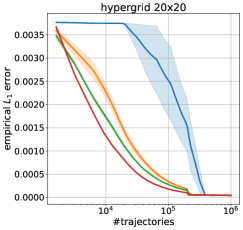
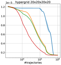
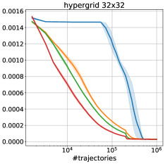
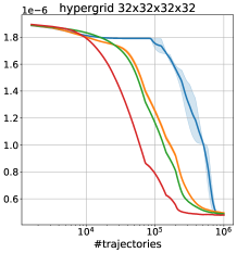
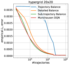
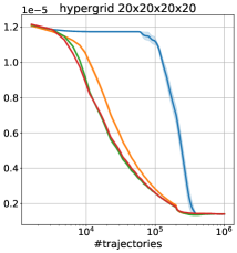
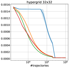
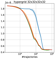
Figure 1: $L_{1}$ distance between target and empirical GFlowNet distributions over the course of training on hypergrid environment. Top row: $\mathcal{P}_{\mathrm{B}}$ is fixed to be uniform for all methods. Bottom row: $\mathcal{P}_{\mathrm{B}}$ is learnt for the baselines and fixed to be uniform for M-DQN. Mean and std values are computed over 3 runs.

In this section we evaluate soft RL approach to the task of GFlowNet training under the proposed paradigm and compare to prior GFlowNet training approaches: trajectory balance (TB, Malkin et al.,, 2022), detailed balance (DB, Bengio et al.,, 2023) and subtrajectory balance (SubTB, Madan et al.,, 2023). Among soft RL methods, for the sake of brevity this sections only presents the results for Munchausen DQN (M-DQN, Vieillard et al., 2020b, ) since we found it to show better performance in comparison to other considered techniques. For ablation studies and additional comparisons we refer the reader to Appendix D.

4.1 Hypergrid Environment

We start with synthetic hypergrid environments introduced in Bengio et al., (2021). These environments are small enough that the normalizing constant $\mathrm{Z}$ can be computed exactly and the trained policy can be efficiently evaluated against the true distribution of interest.

The set of non-terminal states is a set of points with integer coordinates inside a $D$-dimensional hypercube with side length $H$: $\mathopen{}\mathclose{{}\left\{\mathopen{}\mathclose{{}\left(s^{1},\ldots,s^{D}}\right)\mid s^{i}\in\{0,1,\ldots,H-1\}}\right\}$. The initial state is $(0,\ldots,0)$, and for each non-terminal state $s$ there is its copy $s^{\mathsf{\scriptscriptstyle T}}$ which is terminal. For a non-terminal state $s$ the allowed actions are incrementing one coordinate by $1$ without exiting the grid and the terminating action $s\to s^{\mathsf{\scriptscriptstyle T}}$. The reward has modes near the corners of the grid which are separated by wide troughs with a very small reward. We study 2-dimensional and 4-dimensional grids with reward parameters taken from Malkin et al., (2022). To measure the performance of GFlowNet during training, $L_{1}$-distance is computed between the true reward distribution $\mathcal{R}(x)/\mathrm{Z}$ and the empirical distribution $\pi(x)$ of last $2\cdot 10^{5}$ samples seen in training (endpoints of trajectories sampled from $\mathcal{P}_{\mathrm{F}}$): $\frac{1}{|\mathcal{X}|}\sum_{x\in\mathcal{X}}|\mathcal{R}(x)/\mathrm{Z}-\pi(x)|$. Remember, that in case of M-DQN we have $\mathcal{P}_{\mathrm{F}}(\cdot\mid s)=\mathrm{Softmax}_{\lambda}(Q_{\theta}(s,\cdot))$ for $\lambda=1/(1-\alpha)$. All models are parameterized by MLP that accepts a one-hot encoding of $s$ as input. Additional details can be found in Appendix C.1.

We consider two cases for the baselines: uniform and learnt $\mathcal{P}_{\mathrm{B}}$. Since our theoretical framework does not support learnt $\mathcal{P}_{\mathrm{B}}$, we fix it to be uniform for M-DQN in all cases. Figure 1 presents the results. M-DQN has faster convergence than all baselines in case of uniform $\mathcal{P}_{\mathrm{B}}$. Training $\mathcal{P}_{\mathrm{B}}$ improves the speed of convergence for the baselines, with SubTB showing better performance than M-DQN in some cases. However, even with learnt $\mathcal{P}_{\mathrm{B}}$, TB and DB converge slower than M-DQN.

4.2 Small Molecule Generation

Next, we consider the molecule generation task from Bengio et al., (2021). The goal is to generate binders of the sEH (soluble epoxide hydrolase) protein. The molecules represented by graphs are generated by sequentially joining parts from a predefined vocabulary of building blocks (Jin et al.,, 2020). The state space size is approximately $10^{16}$ and each state has between $100$ and $2000$ possible actions. The reward is based on a docking prediction (Trott and Olson,, 2010) and is given in a form of pre-trained proxy model $\tilde{\mathcal{R}}$ from Bengio et al., (2021). Additionally, the reward exponent hyperparameter $\beta$ is introduced, so the GFlowNet is trained using the reward $\mathcal{R}(x)=\tilde{\mathcal{R}}(x)^{\beta}$.

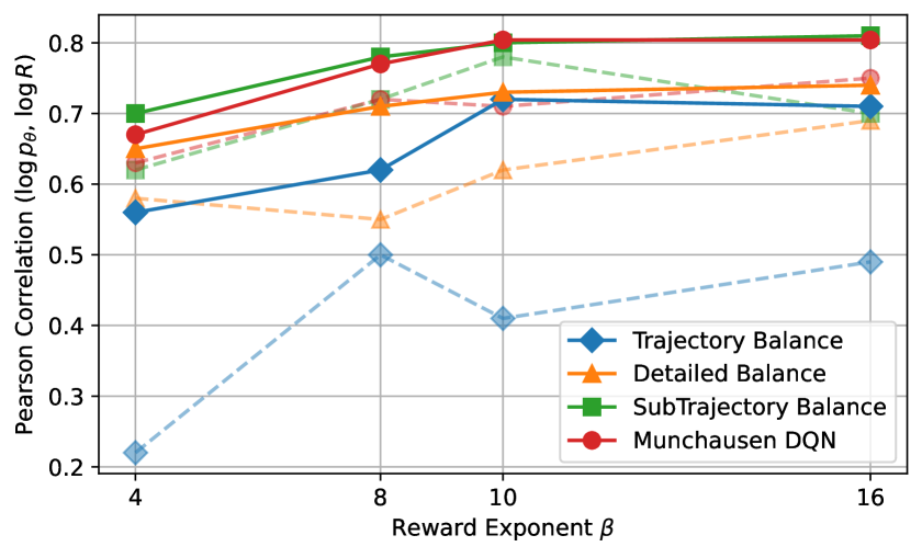
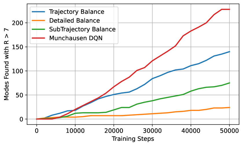
Figure 2: Small molecule generation results. Above: Pearson correlation between $\log\mathcal{R}$ and $\log\mathcal{P}_{\theta}$ on a test set for each method and varying $\beta\in\{4,8,10,16\}$. Solid lines represent the best results over choices of learning rate, dashed lines — mean results. Below: Number of Tanimoto-separated modes with $\tilde{\mathcal{R}}>7.0$ found over the course of training for $\beta=10$.

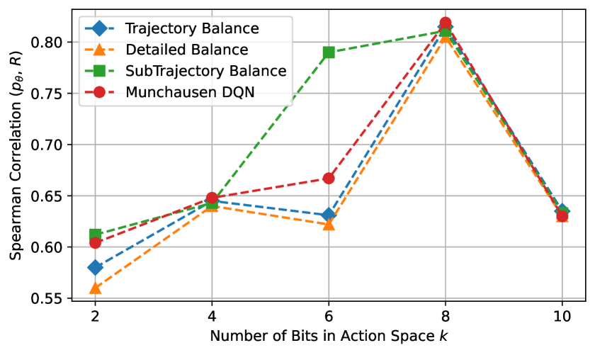
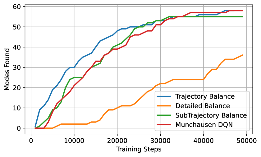
Figure 3: Bit sequence generation results. Above: Spearman correlation between $\mathcal{R}$ and $\mathcal{P}_{\theta}$ on a test set for each method and varying $k\in\{2,4,6,8,10\}$. Below: The number of modes discovered over the course of training for $k=8$.

We follow the setup from Madan et al., (2023). Each model is trained with different values of learning rate and $\beta$. $\mathcal{P}_{\mathrm{B}}$ is fixed to be uniform for all methods. To measure how well the trained models match the target distribution, Pearson correlation is computed on a fixed test set of molecules between $\log\mathcal{R}(x)$ and $\log\mathcal{P}_{\theta}(x)$, where the latter is log probability that $x$ is the end of a trajectory sampled from $\mathcal{P}_{\mathrm{F}}$. $\log\mathcal{P}_{\theta}(x)$ is estimated the same way as in Madan et al., (2023). Additionally, we track the number of Tanimoto-separated modes captured by each method over the course of training as proposed in Bengio et al., (2021). Further experimental details are given in Appendix C.2.

The results are presented in Figure 2. We find that M-DQN outperforms TB and DB in terms of reward correlation and shows similar (or slightly worse when $\beta=4$) performance when compared to SubTB. It also has a similar robustness to the choice of learning rate when compared to SubTB. However, M-DQN discovers more modes over the course of training than all baselines.

4.3 Non-Autoregressive Sequence Generation

Finally, we consider the bit sequence generation task from Malkin et al., (2022) and Madan et al., (2023). To create a harder GFlowNet learning task with non-tree DAG structure, we modify the state and action spaces, allowing non-autoregressive generation akin to the approach used in Zhang et al., 2022b .

The goal is to generate binary strings of a fixed length $n=120$. The reward is specified by the set of modes $M\subset\mathcal{X}=\{0,1\}^{n}$ and is defined as $\mathcal{R}(x)=\exp(-\min_{x^{\prime}\in M}d(x,x^{\prime}))$, where $d$ is Hamming distance. We construct $M$ the same way as in Malkin et al., (2022) and use $|M|=60$. Parameter $k$ is introduced as a tradeoff between trajectory length and action space sizes. For varying $k\mid n$, the vocabulary is defined as a set of all $k$-bit words. The generation starts at a sequence of $n/k$ special "empty" words $\oslash$, and at each step the allowed actions are to pick any position with an empty word and replace it with some word from the vocabulary. Thus the state space consists of sequences of $n/k$ words, having one of $2^{k}+1$ possible words at each position. The terminal states are the states with no empty words, thus corresponding to binary strings of length $n$.

To evaluate the model performance, we utilize two metrics used in Malkin et al., (2022) and Madan et al., (2023) for this task: 1) test set Spearman correlation between $\mathcal{R}(x)$ and $\mathcal{P}_{\theta}(x)$ 2) number of modes captured during training (number of bit strings from $M$ for which a candidate within a distance $\delta=30$ has been generated). In contrast to the setup in Malkin et al., 2023a , the exact probability of sampling $x$ from GFlowNet is intractable in our case due to a large number of paths leading to each $x$, so we utilize a Monte Carlo estimate proposed in Zhang et al., 2022b . We fix $\mathcal{P}_{\mathrm{B}}$ to be uniform in our experiments. Additional details can be found in Appendix C.3.

Figure 3 presents the results. M-DQN has similar or better reward correlation than all baselines except in the case of $k=6$, where it ouperforms TB and DB but falls behind SubTB. In terms of discovered modes, it shows better performance than DB and similar performance to TB and SubTB.

5 CONCLUSION AND FURTHER WORK

In this paper we established a direct connection between GFlowNets and entropy-regularized RL in the general case and experimentally verified it. If a GFlowNet backward policy is fixed, an MDP is appropriately constructed from a GFlowNet DAG and specific rewards are set for all transitions, we showed that learning the GFlowNet forward policy $\mathcal{P}_{\mathrm{F}}$ is equivalent to learning the optimal RL policy $\pi^{\star}_{\lambda}$ when entropy regularization coefficient $\lambda$ is set to $1$. In our experiments, we demonstrated that M-DQN (Vieillard et al., 2020b, ) shows competitive results when compared to established GFlowNet training methods (Malkin et al.,, 2022; Bengio et al.,, 2023; Madan et al.,, 2023) and even outperforms them in some cases.

A promising direction for further research is to explore theoretical properties of GFlowNets by extending analysis of Wen and Van Roy, (2017). Additionally, it would be valuable to generalize the established connection beyond the discrete setting, following the work of Lahlou et al., 2023a . Furthermore, from the practical perspective there is an interesting direction of extending Monte-Carlo Tree Search-based (MCTS) algorithms to GFlowNets such as AlphaZero (Silver et al.,, 2018) since known deterministic environment allows to perform MCTS rollouts.

Finally, in the context of existing connections between GFlowNets and 1) generative modeling (Zhang et al., 2022a, ), 2) Markov Chain Monte Carlo methods (Deleu and Bengio,, 2023), 3) variational inference (Malkin et al., 2023b, ), with addition of the presented link to 4) reinforcement learning, another interesting direction can be to view GFlowNets as a unifying point of different ML areas and models, which can lead to further establishment of new valuable connections.

Appendix A NOTATION

Table 1: Table of notation used throughout the paper.

Notation	Meaning
$\mathcal{S}$	state space
$\mathcal{A}$	action space
$\mathcal{X}$	sampling space
$\mathcal{R}$	GFlowNet reward function
$\mathcal{F}(\tau),\mathcal{F}(s),\mathcal{F}(s\to s^{\prime})$	flow function
$\mathcal{P}(\tau)$	probability over trajectories induced by a flow
$\mathcal{P}(x)$	probability over terminal states of trajectories
$\mathcal{P}_{\mathrm{F}}(s^{\prime}|s)$	forward Markovian policy
$\mathcal{P}_{\mathrm{B}}(s|s^{\prime})$	backward Markovian policy
$\mathrm{Z},\mathrm{Z}_{\mathcal{F}}$	normalizing constant of the reward distribution and a flow $\mathcal{F}$
$\mathrm{P}(s^{\prime}|s,a)$	Markovian transition kernel for MDP
$r(s,a)$	MDP reward function
$\lambda$	regularization coefficient
$V^{\pi}_{\lambda}(s),Q^{\pi}_{\lambda}(s,a)$	regularized value and Q-value of a given policy $\pi$
$V^{\star}_{\lambda}(s),Q^{\star}_{\lambda}(s,a)$	regularized value and Q-value of an optimal policy
$V^{\pi}(s),Q^{\pi}(s,a)$	regularized value and Q-value of a given policy $\pi$ with coefficient $1$
$V^{\star}(s),Q^{\star}(s,a)$	regularized value and Q-value of an optimal policy with coefficient $1$
$\pi^{\star}_{\lambda}(a|s)$	regularized optimal policy
$q^{\pi}(\tau)$	distribution over trajecories induced by a policy $\pi$
$d^{\pi}(x)$	distribution over terminal states induced by a policy $\pi$
$\mathrm{Softmax}_{\lambda}$	softmax function with a temperature $\lambda>0$, for $x\in\mathbb{R}^{d}$
	$[\mathrm{Softmax}_{\lambda}(x)]_{i}\triangleq{\rm e}^{x_{i}/\lambda}/(\sum_{j=1}^{d}{\rm e}^{x_{j}/\lambda})\ \forall i\in[d]$
$\mathrm{LogSumExp}_{\lambda}$	log-sum-exp function with a temperature $\lambda>0$, for $x\in\mathbb{R}^{d}$
	$\mathrm{LogSumExp}(x)\triangleq\lambda\log(\sum_{i=1}^{d}{\rm e}^{x_{i}/\lambda})$.
$\mathcal{H}$	Shannon entropy function, $\mathcal{H}(p)\triangleq\sum_{i=1}^{n}p_{i}\log(1/p_{i})$.

Let $(\mathsf{X},\mathcal{X})$ be a measurable space and $\mathcal{P}(\mathsf{X})$ be the set of all probability measures on this space. For $p\in\mathcal{P}(\mathsf{X})$ we denote by $\mathbb{E}_{p}$ the expectation w.r.t. $p$. For random variable $\xi:\mathsf{X}\to\mathbb{R}$ notation $\xi\sim p$ means $\operatorname{Law}(\xi)=p$.

For any $p,q\in\mathcal{P}(\mathsf{X})$ the Kullback-Leibler divergence $\operatorname{KL}(p,q)$ is given by

$$\operatorname{KL}(p,q)\triangleq\begin{cases}\mathbb{E}_{p}\mathopen{}\mathclose{{}\left[\log\frac{{\rm d}p}{{\rm d}q}}\right],&p\ll q,\\ +\infty,&\text{otherwise.}\end{cases}$$

Appendix B DETAILED ALGORITHM DESCRIPTION

In this section we provide a detailed algorithmic description of SoftDQN and MunchausenDQN and discuss an effect of several hyperparameters.

B.1 Soft DQN

The pipeline of this algorithm is following. In the start of the learning procedure we have two neural networks: $Q_{\theta}$ and $Q_{\bar{\theta}}$, and $\bar{\theta}=\theta$.

Algorithm 1 SoftDQN (Haarnoja et al.,, 2017) / MunchausenDQN (Vieillard et al., 2020b, )

1:  Input: trajectory budget $N$, number of trajectories on one update $M$, exploration parameter $\varepsilon$, backward kernel $\mathcal{P}_{\mathrm{B}}$, PER $\mathcal{B}$, PER batch size $B$, hard update parameter $T$, soft update parameter $\tau$, Munchausen parameters $\alpha$ ,$l_{0}$;

2:  Initialize parameters of online network $\theta$ and target network $\bar{\theta}=\theta$;

3:  Define entropy coefficient $\lambda=1\ ({\color[rgb]{0,0,1}1/(1-\alpha)})$

4:  for  $t=1,\ldots,\lceil N/M\rceil$ do

5:     Sample $M$ trajectories interaction with $\varepsilon$-greedy version of policy $\pi_{\theta}=\mathrm{Softmax}_{\lambda}(Q_{\theta})$, and place them into replay buffer $\mathcal{B}$;

6:     Sample $B$ transitions $\{(s_{k},a_{k},R_{k},s^{\prime}_{k},d_{k})\}_{k=1}^{N}$ from PER $\mathcal{B}$, where $d_{k}$ is a DONE flag: $d_{k}=\mathds{1}\{s_{k}\in\mathcal{X}\}$, and $R_{k}$ is GflowNet reward is $d_{k}=1$ and $0$ otherwise;

7:     Compute MDP rewards: $r_{k}=d_{k}\log R_{k}+(1-d_{k})\log\mathcal{P}_{\mathrm{B}}(s_{k}|s^{\prime}_{k})$ with a convention $0\log 0=0$ for all $k\in\{1,\ldots,B\}$.

8:     Compute TD targets

$$y_{k}=r_{k}+(1-d_{k})\mathrm{LogSumExp}_{\lambda}\mathopen{}\mathclose{{}\left(Q_{\bar{\theta}}(s^{\prime}_{k})}\right){\color[rgb]{0,0,1}+\alpha\max\{\lambda\log\pi_{\bar{\theta}}(a_{k}|s_{k}),l_{0}\}}$$

optionally using a convention $\mathrm{LogSumExp}_{\lambda}\mathopen{}\mathclose{{}\left(Q_{\bar{\theta}}(s^{\prime}_{k})}\right)=\log\mathcal{R}(s^{\prime}_{k})$ $\forall s^{\prime}_{k}\in\mathcal{X}$ (see explanation below);

9:     Use $y_{k}$ to update priorities in PER (Schaul et al.,, 2016) as

$$p_{k}=\ell\mathopen{}\mathclose{{}\left(Q_{\theta}(s_{k},a_{k}),y_{k}}\right),$$

where $\ell$ is a Huber loss (15).

10:     Compute TD loss

$$\mathcal{L}(\theta)=\frac{1}{B}\sum_{k=1}^{B}\ell\mathopen{}\mathclose{{}\left(Q_{\theta}(s_{k},a_{k}),y_{k}}\right),$$

where $\ell$ is a Huber loss (15).

11:     Perform gradient update by $\nabla_{\theta}\mathcal{L}(\theta)$;

12:     if $t\mod T=0$ then

13:        Update target network $\bar{\theta}:=(1-\tau)\bar{\theta}+\tau\theta$;

14:     end if

15:  end for

16:  Output policy $\pi_{\theta}$.

On each iteration of the algorithm, several trajectories (usually 4 or 16) are sampled by following a softmax policy $\pi_{\theta}(s)=\mathrm{Softmax}_{\lambda}(Q_{\theta}(s))$ (here $\lambda=1$) using an online network $Q_{\theta}$ with (optionally) an additional $\varepsilon$-greedy exploration.

All these sampled trajectories are separated onto transitions $(s_{t},a_{t},s_{t+1},R_{t},d_{t})$, where $R_{t}=\log\mathcal{R}(s_{t})$ if $s_{t}\in\mathcal{X}$ and zero otherwise, $d_{t}=\mathds{1}\{s_{t}\in\mathcal{X}\}$ is a DONE float, and $s_{t+1}$ for $s_{t}\in\mathcal{X}$ can be arbitrary state. Note that we always have $a_{t}=s_{t+1}$, and $a_{t}$ is used solely for the purpose of consistency with common RL notation. These separated transitions are placed into a replay buffer $\mathcal{B}$ (Lin,, 1992) with prioritization mechanism following Schaul et al., (2016).

Next, for a batch of transitions $\{(s_{k},a_{k},s^{\prime}_{k},R_{k},d_{k})\}_{k=1}^{B}$ is sampled from a replay buffer $\mathcal{B}$ using prioritization. MDP rewards are computed as $r_{k}=d_{k}\log\mathcal{R}(s_{k})+(1-d_{k})\log\mathcal{P}_{\mathrm{B}}(s_{k}|s^{\prime}_{k})$, and TD-targets are computed as follows

$$\forall k\in[B]:y_{k}=r_{k}+(1-d_{k})\mathrm{LogSumExp}_{\lambda}(Q_{\bar{\theta}}(s^{\prime}_{k})),$$ (14)

where $\lambda=1$.

Alternatively, one can fully skip transitions that lead to the sink state $s_{f}$ (transitions for which $d_{k}=1$), and instead substitute $\mathrm{LogSumExp}_{\lambda}(Q_{\bar{\theta}}(s^{\prime}_{k}))=\log\mathcal{R}(s^{\prime}_{k})$. This can be done since we know the exact value of $V^{\star}(s)$ for all $s\in\mathcal{X}$. We follow this choice in our experiments.

Given targets, we update priorities for a sampled batch in replay buffer and compute the regression TD-loss as follows

$$\mathcal{L}(\theta)=\frac{1}{B}\sum_{k=1}^{B}\ell(Q_{\theta}(s_{k},a_{k}),y_{k}),$$

where $\ell$ is a Huber loss

$$\ell(x,y)=\begin{cases}\frac{1}{2}(x-y)^{2}&|x-y|\leq 1\\ |x-y|-1/2&|x-y|\geq 1.\end{cases}$$ (15)

Finally, at the end of each iteration we perform either a hard update by copying weights of an online network to weights of the target network following original DQN approach (Mnih et al.,, 2015), or a soft update by applying Polyak averaging with a parameter $\tau<1$ following DDPG approach (Silver et al.,, 2014; Lillicrap et al.,, 2015).

The detailed description of this algorithm is also provided in Algorithm 1. Notice that the complexity of this algorithm is linear in a number of sampled transitions since the size of the buffer is fixed during the training.

Next we discuss some elements of this pipeline in more detail.

Prioritized experience replay

The essence of prioritized experience replay by (Schaul et al.,, 2016) is to sample observations from replay buffer not uniformly but according to priorities that are computes as follows

$$\mathrm{P}(i)=\frac{|p_{i}|^{\alpha}}{\sum_{i\in\mathcal{B}}|p_{i}|^{\alpha}},$$

where $\mathrm{P}(i)$ is a probability to sample $i$-th transition in the replay buffer $\mathcal{B}$, $p_{i}$ is a priority that is equal to last computed TD-error for this transition, and $\alpha$ is a temperature parameter that interpolates between uniform sampling $\alpha=0$ and pure prioritization $\alpha=+\infty$. A typically chosen value of $\alpha$ is between $0.4$ and $0.6$, however, for two experiments (molecule and bit sequence generation) we found more beneficial to select an aggressive value $\alpha=0.9$ to collect hard examples faster.

Additionally, authors of (Schaul et al.,, 2016) applied importance-sampling (IS) correction since the theory prescribes to sample uniformly over the buffer due to stochastic next state $s^{\prime}_{k}$. Smoothed correction is controlled with a coefficient $\beta$ that should be annealed to $1$ over the course of training.

However, in the setup of GFlowNets we noticed that this correction is not needed since the next transition and reward are always deterministic, therefore it is possible to set $\beta$ to be a small constant without any lose of convergence properties. We set $\beta=0.0$ in the hypergrid experiment and $\beta=0.1$ in molecule and bit sequence generation experiments and found it more beneficial than doing higher IS-correction.

Choice of loss

We examine two types of regression losses: classic MSE loss and Huber loss that was applied in DQN (Mnih et al.,, 2015) and MunchausenDQN (Vieillard et al., 2020b, ). The main idea behind the Huber loss is automatic gradient clipping for too large updates. We observed such benefits as more stable training while using Huber loss, thus we use it in all our experiments except some ablation studies in Appendix D.

B.2 Munchausen DQN

All the differences between SoftDQN and M-DQN in the context of GFlowNets are:

• Two additional parameters: $\alpha$ and truncation parameter $l_{0}$;

• Using entropy coefficient $\lambda$ equal to $1/(1-\alpha)$ instead of just $\lambda=1$. In particular, it changes how a policy $\pi_{\theta}(s)=\mathrm{Softmax}_{1/(1-\alpha)}(Q_{\theta}(s))$ and a value $V_{\theta}(s)=\mathrm{LogSumExp}_{1/(1-\alpha)}(Q_{\theta}(s))$ are computed.

• Additional term $\alpha\max\{\lambda\log\pi_{\bar{\theta}}(a_{k}|s_{k}),l_{0}\}$ in the computations of TD-target (14).

All these differences are highlighted in Algorithm 1 with a blue color. The use of a different entropy coefficient is justified by Theorem 1 of Vieillard et al., 2020b since M-DQN with entropy coefficient $\lambda$ and Munchausen coefficient $\alpha$ is equivalent to solving entropy regularized RL with a coefficient $(1-\alpha)\lambda$.

Appendix C EXPERIMENTAL DETAILS

In this section we provided additional details for experiments from Section 4.

C.1 Hypergrids

The reward at $s^{\mathsf{\scriptscriptstyle T}}=(s^{1},\ldots,s^{D})^{\mathsf{\scriptscriptstyle T}}$ is formally defined as

$$\mathcal{R}(s^{\mathsf{\scriptscriptstyle T}})=R_{0} +R_{1}\prod_{i=1}^{D}\mathbb{I}\mathopen{}\mathclose{{}\left[0.25<\mathopen{}\mathclose{{}\left|\frac{s^{i}}{H-1}-0.5}\right|}\right]$$

$$+R_{2}\prod_{i=1}^{D}\mathbb{I}\mathopen{}\mathclose{{}\left[0.3<\mathopen{}\mathclose{{}\left|\frac{s^{i}}{H-1}-0.5}\right|<0.4}\right],$$

where $0<R_{0}\ll R_{1}<R_{2}$. This reward has modes near the corners of the grid which are separated by wide troughs with very small reward of $R_{0}$. In Section 4 we use reward parameters $(R_{0}=10^{-3},R_{1}=0.5,R_{2}=2.0)$ taken from Malkin et al., (2022).

All models are parameterized by MLP of the same architecture as in Bengio et al., (2021) with 2 hidden layers and 256 hidden size. Following Malkin et al., (2022), we train all models with Adam optimizer and use learning rate of $10^{-3}$ and batch size 16 (number of trajectories sampled at each training step). In case of TB, we use learning rate of $10^{-1}$ for $\mathrm{Z}_{\theta}$ following Malkin et al., (2022). For SubTB parameter $\lambda$ (not to be confused with soft RL regularization coefficient) we use the value of $0.9$ following Madan et al., (2023). All models are trained until $10^{6}$ trajectories are sampled and the empirical sample distribution $\pi(x)$ is computed over last $2\cdot 10^{5}$ samples seen in training, which explains the drop in plots at $2\cdot 10^{5}$ mark (see Figure 1).

For M-DQN we use Huber loss instead of MSE, following Mnih et al., (2015); Vieillard et al., 2020b and priortized replay buffer (Schaul et al.,, 2016) from TorchRL library (Bou et al.,, 2023) of size $100,000$, a standard constant $\alpha=0.5$ and without IS correction $\beta=0$. At each training step, we sample 16 trajectories, put all transitions to the buffer, and then sample 256 transitions from the buffer to calculate the loss. Thus M-DQN uses the same number of trajectories and the same number of gradient steps for training as the baselines. Regarding specific Munchausen parameters (Vieillard et al., 2020b, ), we use $\alpha=0.15$ and unusual large $l_{0}=-100$, since the entropy coefficient for our setup is much larger than one that was used in original M-DQN. To update target network we utilize soft updates akin to celebrated DDPG (Silver et al.,, 2014; Lillicrap et al.,, 2015) with a large coefficient $\tau=0.25$ due to sampling $16$ trajectories prior to obtaining a batch.

For hypergrid environment experiments we utilized torchgfn library (Lahlou et al., 2023b, ). All experiments were performed on CPUs.

C.2 Molecules

All models are parameterized with MPNN (Gilmer et al.,, 2017), for which we use the same paramaters as in previous works (Bengio et al.,, 2021; Malkin et al.,, 2022; Madan et al.,, 2023). The reward proxy and the test set are alson taken from Bengio et al., (2021). Following Madan et al., (2023), we consider reward exponents from $\{4,8,10,16\}$, learning rates from $\{5\cdot 10^{-5},10^{-4},5\cdot 10^{-4},10^{-3}\}$ and train all models for 50,000 iterations with batch size 4 using Adam optimizer. For SubTB we use the same value $\lambda=1.0$ as in Madan et al., (2023). Reward correlations for the baselines in Figure 2 are taken directly from Madan et al., (2023). We track Tanimoto-separated modes as described in Bengio et al., (2021), using raw reward threshold of $7.0$ and Tanimoto similarity threshold of $0.7$.

Regarding M-DQN, we use Huber loss instead of MSE, following Mnih et al., (2015); Vieillard et al., 2020b and find great benefits from utilizing dueling architecture (Wang et al.,, 2016), that builds similarity with DB (see Section 3.4). Also we utilize prioritized replay buffer (Schaul et al.,, 2016) from TorchRL library (Bou et al.,, 2023) of size $1,000,000$, and unusual parameters $\alpha=0.9,\beta=0.1$ (see Appendix B for details on this choice), and use Munchausen parameters $\alpha=0.15$ and $l_{0}=-2500$. At each training step, we sample 4 trajectories, put all transitions to the buffer, and then sample 256 transitions from the buffer to calculate the loss. To update target network, we utilize soft updates akin to DDPG (Silver et al.,, 2014; Lillicrap et al.,, 2015) with a coefficient $\tau=0.1$. Notice that M-DQN samples exactly the same number of trajectories for training as the baselines, thus the comparison in terms of discovered modes is fair.

Our experiments are based upon the published code of Bengio et al., (2021) and Malkin et al., (2022). We utilized a cluster with NVIDIA V100 and NVIDIA A100 GPUs for molecule generation experiments.

C.3 Bit Sequences

Mode set $M$ and the test set are constructed as described in Malkin et al., (2022). We also use the same Transformer (Vaswani et al.,, 2017) neural network architecture for all models with 3 hidden layers, 64 hidden dimension and 8 attention heads, with the only difference from Malkin et al., (2022) that it outputs logits for a larger action space since we generate sequences non-autoregressively.

To approximate $\mathcal{P}_{\theta}(x)$ we use the Monte Carlo estimate proposed in Zhang et al., 2022b :

$$\mathcal{P}(x)=\mathbb{E}_{\mathcal{P}_{\mathrm{B}}(\tau\mid x)}\frac{\mathcal{P}_{\mathrm{F}}(\tau)}{\mathcal{P}_{\mathrm{B}}(\tau\mid x)}\approx\frac{1}{N}\sum\limits_{i=1}^{N}\frac{\mathcal{P}_{\mathrm{F}}(\tau^{i})}{\mathcal{P}_{\mathrm{B}}(\tau^{i}\mid x)},$$

where $\mathcal{P}_{\mathrm{F}}(\tau)=\prod_{t=1}^{n_{\tau}}\mathcal{P}_{\mathrm{F}}\mathopen{}\mathclose{{}\left(s_{t}|s_{t-1},\theta}\right)$, $\mathcal{P}_{\mathrm{B}}(\tau\mid x)=\prod_{t=1}^{n_{\tau}}\mathcal{P}_{\mathrm{B}}\mathopen{}\mathclose{{}\left(s_{t-1}|s_{t}}\right)$ and $\tau^{i}\sim\mathcal{P}_{\mathrm{B}}(\tau\mid x)$. Zhang et al., 2022b showed that even with $N=10$ this approach can provide an adequate estimate, so we use this value in our experiments.

We train all models for 50,000 iterations with batch size 16 using Adam optimizer. For all methods the trajectories are sampled using the mixture of $\mathcal{P}_{\mathrm{F}}$ and a uniform distribution over next possible actions, the latter having weight $10^{-3}$ ($\varepsilon$-greedy exploration). We set reward exponent value to $2$. For M-DQN and all baselines we pick the best learning rate from $\{5\times 10^{-4},10^{-3},2\times 10^{-3}\}$. For SubTB we pick the best $\lambda$ from $\{0.9,1.1,1.5,1.9\}$.

For M-DQN we use Huber loss instead of MSE, following (Mnih et al.,, 2015; Vieillard et al., 2020b, ) and priortized replay buffer (Schaul et al.,, 2016) from TorchRL library (Bou et al.,, 2023) of size $100,000$, and constants $\alpha=0.9,\beta=0.1$. At each training step, we sample 16 trajectories and put all transitions to the buffer, and then sample 256 transitions from the buffer to calculate the loss. Regarding specific Munchausen parameters (Vieillard et al., 2020b, ), we use $\alpha=0.15$ and $l_{0}=-25$. We only use hard updates for the target network (Mnih et al.,, 2015) with the frequency of $5$ iterations. Notice that M-DQN samples exactly the same number of trajectories for training as the baselines, thus the comparison in terms of discovered modes is fair. Additionally, for M-DQN we found it helpful to increase the weight of the loss for edges leading to terminal states, which was also done in the original GFlowNet paper (Bengio et al.,, 2021) for flow matching objective, and pick the best weight coefficient from $\{2,5\}$ in our experiments.

For bit sequence experiments we used our own code implementation in PyTorch (Paszke et al.,, 2019). We also utilized a cluster with NVIDIA V100 and NVIDIA A100 GPUs.

Appendix D ADDITIONAL COMPARISONS

In this sections we provide additional experimental comparisons and ablation studies.

D.1 Hypergrids with Hard Reward

We provide experimental results for hypergrids with a harder reward variant proposed in Madan et al., (2023), which has parameters $(R_{0}=10^{-4},R_{1}=1.0,R_{2}=3.0)$. We follow the same experimental setup as in Section 4. The results are presented in Figure 4. We make similar observations to the ones described in Section 4: when $\mathcal{P}_{\mathrm{B}}$ is fixed to be uniform for all methods, M-DQN converges faster than the baselines, and when $\mathcal{P}_{\mathrm{B}}$ is learnt for the baselines, M-DQN shows comparable performance to SubTB and outperforms TB and DB. Notably, TB fails to converge in most cases, which coincides with the results presented in Madan et al., (2023).

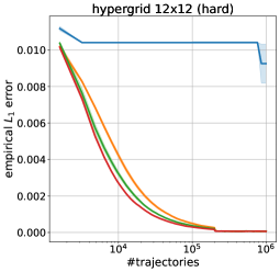
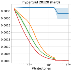
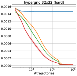
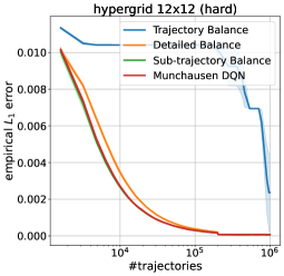
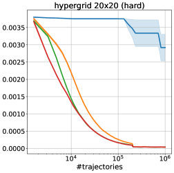
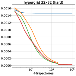
Figure 4: $L_{1}$ distance between target and empirical GFlowNet distributions over the course of training on hypergrid environment for the hard reward variant. Top row: $\mathcal{P}_{\mathrm{B}}$ is fixed to be uniform for all methods. Bottom row: $\mathcal{P}_{\mathrm{B}}$ is learnt for the baselines and fixed to be uniform for M-DQN.

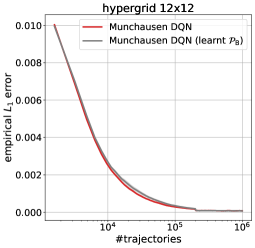
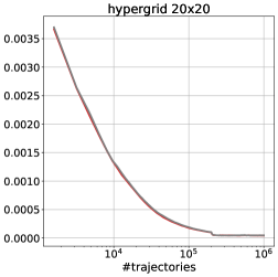
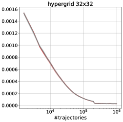
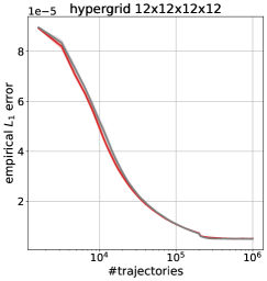
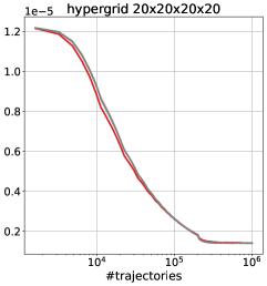
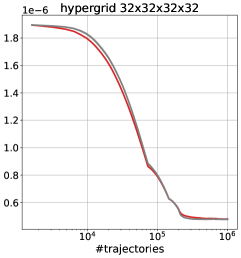
Figure 5: $L_{1}$ distance between target and empirical GFlowNet distributions over the course of training on hypergrid environment. Here we present two versions of M-DQN: one with a fixed uniform $\mathcal{P}_{\mathrm{B}}$ and another one with a learnt $\mathcal{P}_{\mathrm{B}}$ during the training.

D.2 Training Backward Policy

Our theoretical framework does not support running soft RL with a learnable backward policy, thus in Section 4 we used M-DQN with uniform $\mathcal{P}_{\mathrm{B}}$ in all cases. Nevertheless, one can try to use the same M-DQN training loss to calculate gradients and update $\mathcal{P}_{\mathrm{B}}$, thus creating a setup with learnable backward policy. Figure 5 presents the results of comparison on the hypergrid environment (with standard reward, the same as in Section 4). We find that having a trainable $\mathcal{P}_{\mathrm{B}}$ does not improve the speed of convergence for M-DQN, in contrast to the behavior of learnt $\mathcal{P}_{\mathrm{B}}$ in case of previously proposed GFlowNet training methods presented in Figure 1.

Another possible approach to training $\mathcal{P}_{\mathrm{B}}$ in case of soft RL can be to use some other GFlowNet training objective to calculate the loss for $\mathcal{P}_{\mathrm{B}}$, for example TB, while using soft RL to train $\mathcal{P}_{\mathrm{F}}$. We leave this case for the further study.

D.3 Different Soft RL algorithms

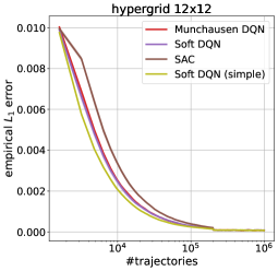
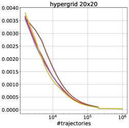
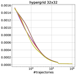
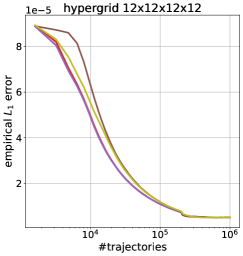
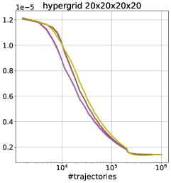
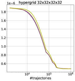
Figure 6: $L_{1}$ distance between target and empirical GFlowNet distributions over the course of training on hypergrid environment. $\mathcal{P}_{\mathrm{B}}$ is fixed to be uniform for all methods. Here we compare different soft RL algorithms.

D.3.1 Hypergrid Environment

We also compare M-DQN to other known off-policy soft RL algorithms:

Soft DQN

To ablate the effect of Munchausen penalty in M-DQN we compare it to a classic version of SoftDQN, which is equivalent to setting Munchausen constant $\alpha=0$. All other hyperparameters are chosen exactly the same as for M-DQN (see Appendix C).

Soft DQN (simple)

To ablate the effect of using a replay buffer and Huber loss, we also train a simplified version of SoftDQN. At each training iteration, it samples a batch of trajectories and uses the sampled transitions to calculate the loss, similarly to the way GFlowNet is trained with DB objective. It also uses MSE loss instead of Huber.

Soft Actor Critic

We also considered SAC (Haarnoja et al.,, 2018) algorithm, namely its discrete counterpart presented by Christodoulou, (2019). We follow the implementation presented in CleanRL library (Huang et al.,, 2022) with two differences: usage of Huber loss (Mnih et al.,, 2015) and lack of tuning of entropy regularization parameter since the theory prescribes to set its value to $1$. All other hyperparameters are chosen exactly the same as for M-DQN and SoftDQN (see Appendix C).

Figure 6 presents the results of comparison on the hypergrid environment (with standard reward, the same as in Section 4). We found that M-DQN and SoftDQN generally have very similar performance, while converging faster than SAC in most cases. Interestingly, the simplified version of SoftDQN holds its own against other algorithms, converging faster on smaller 2-dimensional grids, while falling behind M-DQN and SoftDQN on 4-dimensional ones. This indicates that the success of soft RL is not only due to using replay buffer and Huber loss instead of MSE, but the training objective itself is well-suited for the GFlowNet learning problem.

D.3.2 Small Molecule Generation

We also compare M-DQN and SoftDQN on the molecule generation task. The experimental setup is the same as the one used in Section 4. Figure 7 presents the results. SoftDQN shows worse performance when $\beta=16$ in comparison to M-DQN. But in all other cases, it shows comparable or better reward correlations, and is more robust to the choise of learning rate. However, M-DQN discovers modes faster.

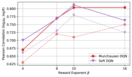
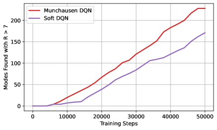
Figure 7: Small molecule generation results. Left: Pearson correlation between $\log\mathcal{R}$ and $\log\mathcal{P}_{\theta}$ on a test set for each method and varying $\beta\in\{4,8,10,16\}$. Solid lines represent the best results over choices of learning rate, dashed lines — mean results. Right: Number of Tanimoto-separated modes with $\tilde{\mathcal{R}}>7.0$ found over the course of training for $\beta=10$.

D.3.3 Bit Sequence Generation

Finally, we compare M-DQN and SoftDQN on the bit sequence generation task. The experimental setup is the same as the one used in Section 4. Figure 8 presents the results. SoftDQN has comparable or worse reward correlations in comparison to M-DQN and discovers modes slightly slower.

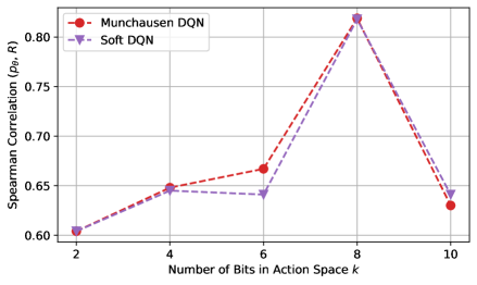
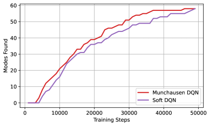
Figure 8: Bit sequence generation results. Left: Spearman correlation between $\mathcal{R}$ and $\mathcal{P}_{\theta}$ on a test set for each method and varying $k\in\{2,4,6,8,10\}$. Right: The number of modes discovered over the course of training for $k=8$.

References

- Bellemare et al., (2016) Bellemare, M., Srinivasan, S., Ostrovski, G., Schaul, T., Saxton, D., and Munos, R. (2016). Unifying count-based exploration and intrinsic motivation. Advances in neural information processing systems, 29.
- Bellemare et al., (2023) Bellemare, M. G., Dabney, W., and Rowland, M. (2023). Distributional Reinforcement Learning. MIT Press. http://www.distributional-rl.org.
- Bengio et al., (2021) Bengio, E., Jain, M., Korablyov, M., Precup, D., and Bengio, Y. (2021). Flow network based generative models for non-iterative diverse candidate generation. Advances in Neural Information Processing Systems, 34:27381–27394.
- Bengio et al., (2023) Bengio, Y., Lahlou, S., Deleu, T., Hu, E. J., Tiwari, M., and Bengio, E. (2023). Gflownet foundations. Journal of Machine Learning Research, 24(210):1–55.
- Bou et al., (2023) Bou, A., Bettini, M., Dittert, S., Kumar, V., Sodhani, S., Yang, X., De Fabritiis, G., and Moens, V. (2023). Torchrl: A data-driven decision-making library for pytorch. arXiv preprint arXiv:2306.00577.
- Burda et al., (2019) Burda, Y., Edwards, H., Storkey, A., and Klimov, O. (2019). Exploration by random network distillation. In International Conference on Learning Representations.
- Christodoulou, (2019) Christodoulou, P. (2019). Soft actor-critic for discrete action settings. arXiv preprint arXiv:1910.07207.
- Cover, (1999) Cover, T. M. (1999). Elements of information theory. John Wiley & Sons.
- Deleu and Bengio, (2023) Deleu, T. and Bengio, Y. (2023). Generative flow networks: a markov chain perspective. arXiv preprint arXiv:2307.01422.
- Deleu et al., (2022) Deleu, T., Góis, A., Emezue, C., Rankawat, M., Lacoste-Julien, S., Bauer, S., and Bengio, Y. (2022). Bayesian structure learning with generative flow networks. In Uncertainty in Artificial Intelligence, pages 518–528. PMLR.
- Fox et al., (2016) Fox, R., Pakman, A., and Tishby, N. (2016). Taming the noise in reinforcement learning via soft updates. In Ihler, A. and Janzing, D., editors, Proceedings of the Thirty-Second Conference on Uncertainty in Artificial Intelligence, UAI 2016, June 25-29, 2016, New York City, NY, USA. AUAI Press.
- Geist et al., (2019) Geist, M., Scherrer, B., and Pietquin, O. (2019). A theory of regularized markov decision processes. In International Conference on Machine Learning, pages 2160–2169. PMLR.
- Gilmer et al., (2017) Gilmer, J., Schoenholz, S. S., Riley, P. F., Vinyals, O., and Dahl, G. E. (2017). Neural message passing for quantum chemistry. In International conference on machine learning, pages 1263–1272. PMLR.
- Haarnoja et al., (2017) Haarnoja, T., Tang, H., Abbeel, P., and Levine, S. (2017). Reinforcement learning with deep energy-based policies. In International conference on machine learning, pages 1352–1361. PMLR.
- Haarnoja et al., (2018) Haarnoja, T., Zhou, A., Abbeel, P., and Levine, S. (2018). Soft actor-critic: Off-policy maximum entropy deep reinforcement learning with a stochastic actor. In Dy, J. and Krause, A., editors, Proceedings of the 35th International Conference on Machine Learning, volume 80 of Proceedings of Machine Learning Research, pages 1861–1870. PMLR.
- Huang et al., (2022) Huang, S., Dossa, R. F. J., Ye, C., Braga, J., Chakraborty, D., Mehta, K., and Araújo, J. G. (2022). Cleanrl: High-quality single-file implementations of deep reinforcement learning algorithms. Journal of Machine Learning Research, 23(274):1–18.
- Jin et al., (2020) Jin, W., Barzilay, R., and Jaakkola, T. (2020). Junction tree variational autoencoder for molecular graph generation. In Artificial Intelligence in Drug Discovery, pages 228–249. The Royal Society of Chemistry.
- (18) Lahlou, S., Deleu, T., Lemos, P., Zhang, D., Volokhova, A., Hernández-Garcıa, A., Ezzine, L. N., Bengio, Y., and Malkin, N. (2023a). A theory of continuous generative flow networks. In International Conference on Machine Learning, pages 18269–18300. PMLR.
- (19) Lahlou, S., Viviano, J. D., and Schmidt, V. (2023b). torchgfn: A pytorch gflownet library. arXiv preprint arXiv:2305.14594.
- Lillicrap et al., (2015) Lillicrap, T. P., Hunt, J. J., Pritzel, A., Heess, N., Erez, T., Tassa, Y., Silver, D., and Wierstra, D. (2015). Continuous control with deep reinforcement learning. arXiv preprint arXiv:1509.02971.
- Lin, (1992) Lin, L.-J. (1992). Self-improving reactive agents based on reinforcement learning, planning and teaching. Machine learning, 8:293–321.
- Madan et al., (2023) Madan, K., Rector-Brooks, J., Korablyov, M., Bengio, E., Jain, M., Nica, A. C., Bosc, T., Bengio, Y., and Malkin, N. (2023). Learning gflownets from partial episodes for improved convergence and stability. In International Conference on Machine Learning, pages 23467–23483. PMLR.
- Malkin et al., (2022) Malkin, N., Jain, M., Bengio, E., Sun, C., and Bengio, Y. (2022). Trajectory balance: Improved credit assignment in gflownets. Advances in Neural Information Processing Systems, 35:5955–5967.
- (24) Malkin, N., Lahlou, S., Deleu, T., Ji, X., Hu, E. J., Everett, K. E., Zhang, D., and Bengio, Y. (2023a). GFlownets and variational inference. In The Eleventh International Conference on Learning Representations.
- (25) Malkin, N., Lahlou, S., Deleu, T., Ji, X., Hu, E. J., Everett, K. E., Zhang, D., and Bengio, Y. (2023b). GFlownets and variational inference. In The Eleventh International Conference on Learning Representations.
- Mnih et al., (2015) Mnih, V., Kavukcuoglu, K., Silver, D., Rusu, A. A., Veness, J., Bellemare, M. G., Graves, A., Riedmiller, M., Fidjeland, A. K., Ostrovski, G., et al. (2015). Human-level control through deep reinforcement learning. nature, 518(7540):529–533.
- Neu et al., (2017) Neu, G., Jonsson, A., and Gómez, V. (2017). A unified view of entropy-regularized markov decision processes. arXiv preprint arXiv:1705.07798.
- Osband et al., (2016) Osband, I., Blundell, C., Pritzel, A., and Van Roy, B. (2016). Deep exploration via bootstrapped dqn. Advances in neural information processing systems, 29.
- Ostrovski et al., (2017) Ostrovski, G., Bellemare, M. G., Oord, A., and Munos, R. (2017). Count-based exploration with neural density models. In International conference on machine learning, pages 2721–2730. PMLR.
- Pan et al., (2023) Pan, L., Zhang, D., Courville, A., Huang, L., and Bengio, Y. (2023). Generative augmented flow networks. In The Eleventh International Conference on Learning Representations.
- Paszke et al., (2019) Paszke, A., Gross, S., Massa, F., Lerer, A., Bradbury, J., Chanan, G., Killeen, T., Lin, Z., Gimelshein, N., Antiga, L., et al. (2019). Pytorch: An imperative style, high-performance deep learning library. Advances in neural information processing systems, 32.
- Rector-Brooks et al., (2023) Rector-Brooks, J., Madan, K., Jain, M., Korablyov, M., Liu, C.-H., Chandar, S., Malkin, N., and Bengio, Y. (2023). Thompson sampling for improved exploration in gflownets. arXiv preprint arXiv:2306.17693.
- Saade et al., (2023) Saade, A., Kapturowski, S., Calandriello, D., Blundell, C., Sprechmann, P., Sarra, L., Groth, O., Valko, M., and Piot, B. (2023). Unlocking the power of representations in long-term novelty-based exploration. arXiv preprint arXiv:2305.01521.
- Schaul et al., (2016) Schaul, T., Quan, J., Antonoglou, I., and Silver, D. (2016). Prioritized experience replay. In Bengio, Y. and LeCun, Y., editors, 4th International Conference on Learning Representations, ICLR 2016, San Juan, Puerto Rico, May 2-4, 2016, Conference Track Proceedings.
- (35) Schulman, J., Chen, X., and Abbeel, P. (2017a). Equivalence between policy gradients and soft q-learning. arXiv preprint arXiv:1704.06440.
- (36) Schulman, J., Wolski, F., Dhariwal, P., Radford, A., and Klimov, O. (2017b). Proximal policy optimization algorithms. arXiv preprint arXiv:1707.06347.
- Shen et al., (2023) Shen, M. W., Bengio, E., Hajiramezanali, E., Loukas, A., Cho, K., and Biancalani, T. (2023). Towards understanding and improving gflownet training. In Proceedings of the 40th International Conference on Machine Learning, ICML’23. JMLR.org.
- Silver et al., (2018) Silver, D., Hubert, T., Schrittwieser, J., Antonoglou, I., Lai, M., Guez, A., Lanctot, M., Sifre, L., Kumaran, D., Graepel, T., Lillicrap, T., Simonyan, K., and Hassabis, D. (2018). A general reinforcement learning algorithm that masters chess, shogi, and go through self-play. Science, 362(6419):1140–1144.
- Silver et al., (2014) Silver, D., Lever, G., Heess, N., Degris, T., Wierstra, D., and Riedmiller, M. (2014). Deterministic policy gradient algorithms. In International conference on machine learning, pages 387–395. Pmlr.
- Sutton, (1988) Sutton, R. S. (1988). Learning to predict by the methods of temporal differences. Machine learning, 3:9–44.
- Sutton and Barto, (2018) Sutton, R. S. and Barto, A. G. (2018). Reinforcement learning: An introduction. MIT press.
- Tang et al., (2023) Tang, Y., Munos, R., Rowland, M., and Valko, M. (2023). VA-learning as a more efficient alternative to q-learning. In Krause, A., Brunskill, E., Cho, K., Engelhardt, B., Sabato, S., and Scarlett, J., editors, Proceedings of the 40th International Conference on Machine Learning, volume 202 of Proceedings of Machine Learning Research, pages 33739–33757. PMLR.
- Tiapkin et al., (2023) Tiapkin, D., Belomestny, D., Calandriello, D., Moulines, E., Munos, R., Naumov, A., Perrault, P., Tang, Y., Valko, M., and Ménard, P. (2023). Fast rates for maximum entropy exploration. In Proceedings of the 40th International Conference on Machine Learning, ICML’23. JMLR.org.
- Trott and Olson, (2010) Trott, O. and Olson, A. J. (2010). Autodock vina: improving the speed and accuracy of docking with a new scoring function, efficient optimization, and multithreading. Journal of computational chemistry, 31(2):455–461.
- Vaswani et al., (2017) Vaswani, A., Shazeer, N., Parmar, N., Uszkoreit, J., Jones, L., Gomez, A. N., Kaiser, Ł., and Polosukhin, I. (2017). Attention is all you need. Advances in neural information processing systems, 30.
- Vemgal et al., (2023) Vemgal, N., Lau, E., and Precup, D. (2023). An empirical study of the effectiveness of using a replay buffer on mode discovery in gflownets. arXiv preprint arXiv:2307.07674.
- (47) Vieillard, N., Kozuno, T., Scherrer, B., Pietquin, O., Munos, R., and Geist, M. (2020a). Leverage the average: an analysis of kl regularization in reinforcement learning. Advances in Neural Information Processing Systems, 33:12163–12174.
- (48) Vieillard, N., Pietquin, O., and Geist, M. (2020b). Munchausen reinforcement learning. Advances in Neural Information Processing Systems, 33:4235–4246.
- Wang et al., (2016) Wang, Z., Schaul, T., Hessel, M., Hasselt, H., Lanctot, M., and Freitas, N. (2016). Dueling network architectures for deep reinforcement learning. In International conference on machine learning, pages 1995–2003. PMLR.
- Wen and Van Roy, (2017) Wen, Z. and Van Roy, B. (2017). Efficient reinforcement learning in deterministic systems with value function generalization. Mathematics of Operations Research, 42(3):762–782.
- Zahavy et al., (2021) Zahavy, T., O’Donoghue, B., Desjardins, G., and Singh, S. (2021). Reward is enough for convex mdps. Advances in Neural Information Processing Systems, 34:25746–25759.
- (52) Zhang, D., Chen, R. T., Malkin, N., and Bengio, Y. (2022a). Unifying generative models with gflownets. arXiv preprint arXiv:2209.02606.
- (53) Zhang, D., Malkin, N., Liu, Z., Volokhova, A., Courville, A., and Bengio, Y. (2022b). Generative flow networks for discrete probabilistic modeling. In International Conference on Machine Learning, pages 26412–26428. PMLR.
- Zhang et al., (2023) Zhang, D., Pan, L., Chen, R. T., Courville, A., and Bengio, Y. (2023). Distributional gflownets with quantile flows. arXiv preprint arXiv:2302.05793.