Unsupervised Object Localization in the Era of Self-Supervised ViTs: A Survey

Abstract

The recent enthusiasm for open-world vision systems show the high interest of the community to perform perception tasks outside of the closed-vocabulary benchmark setups which have been so popular until now. Being able to discover objects in images/videos without knowing in advance what objects populate the dataset is an exciting prospect. But how to find objects without knowing anything about them? Recent works show that it is possible to perform class-agnostic unsupervised object localization by exploiting self-supervised pre-trained features. We propose here a survey of unsupervised object localization methods that discover objects in images without requiring any manual annotation in the era of self-supervised ViTs. We gather links of discussed methods in the repository https://github.com/valeoai/Awesome-Unsupervised-Object-Localization.

1 Introduction

Object localization in 2D images is a key task for many perception systems, e.g. autonomous robots and cars, augmented reality headsets, visual search engines, etc. Depending on the application, the task can take different forms such as object detection [73, 14] and instance segmentation [39, 18]. Achieving good results in these tasks has traditionally hinged on one critical factor: access to extensive, meticulously annotated datasets [59, 31] to build and train deep neural networks.

However, this paradigm comes with inherent limitations. The first obvious one is the high cost and tediousness involved in acquiring these datasets. The second limitation stems from the finite and pre-defined nature of the set of object classes which significantly narrows the scope of what supervised models can perceive and identify. This becomes particularly problematic in contexts where the ability to recognize and respond to unknown or unconventional objects is crucial. For example, in autonomous driving applications, where the road can present a multitude of unpredictable elements, the need to apprehend whatever comes into view is paramount.

Figure 1: Evolution of the number of papers on unsupervised object localization. Histogram of the number of papers mentioning “unsupervised object detection/segmentation/localization” in their title per year, from 2000 to 2022. Data captured by querying dblp.org paper repository.

Figure 2: Performance evolution in unsupervised object localization. Evolution of the CorLoc score (more details in Sec. 2.3) evaluated on VOC07 dataset in the last three years. In green are methods including a self-training stage, when those in orange solely exploit frozen self-supervised features. Brown squares are previous baselines doing dataset level optimization. Results have gained more than 20 pts in 2 years with simpler/faster methods which exploit self-supervised features. ‘Bb ref.[34]⁺⁺’ corresponds to the combination of [34] with MOVE [12] and the training of a class-agnostic detector following [85].

A solution to discover objects of interest without relying on annotations is to perform unsupervised class-agnostic object localization. This challenging task consists in localizing objects in images with no human supervision. Such problem has recently gained a lot of attention as shown by the evolution of the number of papers written about ‘unsupervised object localization’ (see Fig. 1). Moreover, as shown in Fig. 2, recent methods (e.g., MOST [70] and MOVE [12]) have achieved impressive results without any annotations, predicting accurate object boxes in over 75% of the images in the VOC07 [31] dataset.

The recent progress in unsupervised localization tasks owes its success to two critical factors. First, Vision Transformer (ViT) models [29] provide global correlations between patches when Convolutional Neural Networks (CNNs) only correlate pixels in a local receptive field. Second, self-supervised representation learning [16, 22, 40] has improved and scaled to massive datasets for feature learning. These techniques can now extract local and global semantically meaningful features from the weak signal provided by pretext tasks. With such strategies, there is no need to carefully design hand-crafted methods [119, 130], use generative adversarial models [64], refine noisy labels [65], nor to interpret the thousands of object proposals generated by handcrafted methods [132, 90] (with a high-recall but low precision) using expensive dataset-level quadratic pattern repetition search [113, 94, 96, 98].

(a) Unsupervised saliency detection

(b) Single-object discovery

(c) Class-agnostic multi-object detection

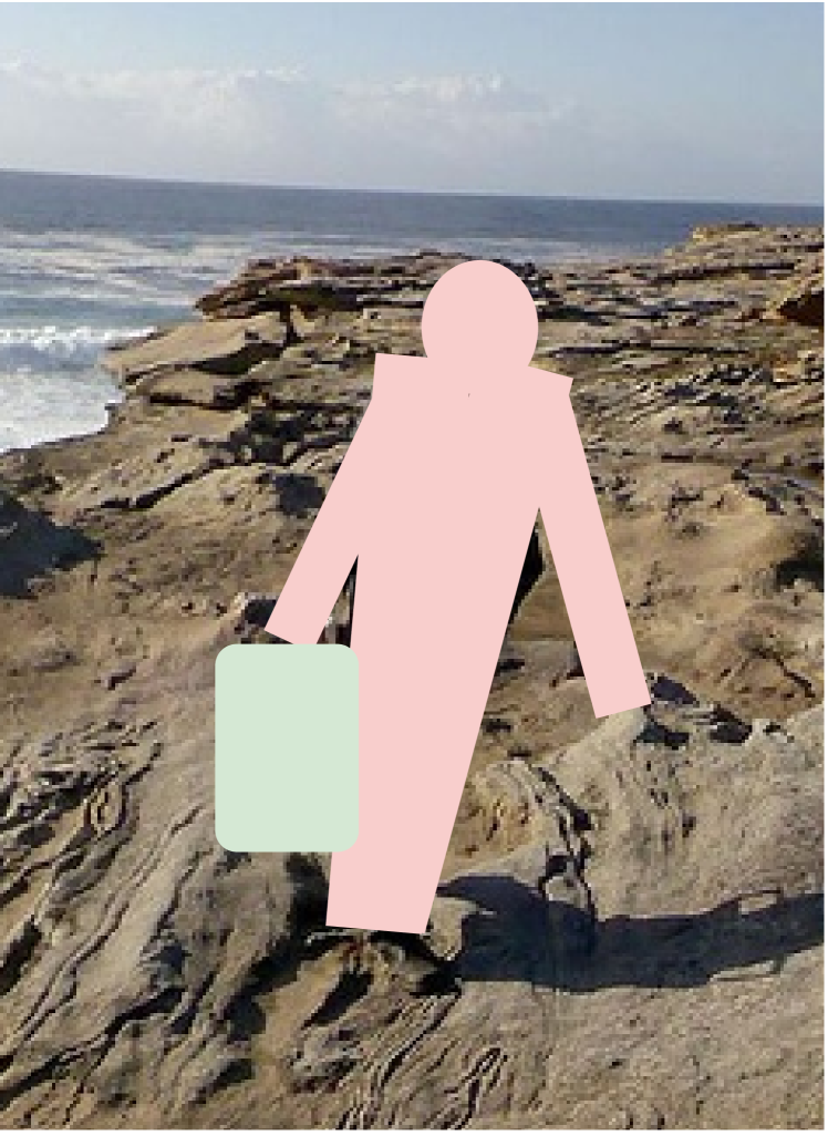
(d) Class-agnostic instance segmentation

Figure 3: The different tasks to evaluate unsupervised object localization methods: (a) unsupervised saliency detection focuses on foreground/background separation, (b) single-object discovery requires to localize well at least a single object with a box, (c) class-agnostic multi-object detection evaluates if all objects have been well detected with good-quality boxes and (d) class-agnostic instance segmentation is the analogue with instance masks.

In this survey, we propose to review unsupervised object localization methods in the era of self-supervised ViTs. We thoroughly present and detail all recent methods addressing this topic and comprehensively organize them for the community. These methods are summarized in Tab. 1. To our knowledge, this is the first survey on such topic and we would like to point the reader to related surveys on image classification with limited annotations [77], weakly supervised object localization [123, 79], object localization on natural scenes [26], instance segmentation [80], object segmentation [110], object detection [3, 81] and open-vocabulary detection and segmentation [129, 115]. Instead, our survey focuses solely on unsupervised methods for object localization.

The survey is organized as follows (state-of-the-art results are gathered in Sec. 4.5):

• Sec. 2: We comprehensively present the different tasks used to evaluate object localization capabilities, as shown in Fig. 3, as well as the corresponding metrics and typical datasets used to evaluate the methods.

• Sec. 3: We review modern solutions that exploit ViT self-supervised features to produce localization masks in a training-free way.

• Sec. 4: We detail different self-training strategies employed to enhance the quality of coarse localization mined in the self-supervised features.

• Sec. 5: We discuss the success and failures of presented methods and open to different means to obtain object localization information without manual annotation.

Method	Sec.	Code available	Venue	Unsupervised saliency detection	Single-object discovery	Class-agnostic multi-object detection	Class-agnostic multi-object segmentation
DINO [16]	3.2	✓	ICCV 2021	—	[xx]✓[85]	—	[xx]✓[33]
LOST [85]	3.3.2, 4.2	✓	BMVC 2021	[xx]✓[111]	✓	✓	[xx]✓[33]
SelfMask [83]	3.3.3, 4.1.2	✓	CVPRW 2022	✓	[xx]✓[86]	—	—
DSM [63]	3.3.3	✓	CVPR 2022	✓	✓	—	—
FreeSOLO [107]	3.4.4, 4.3	✓	CVPR 2022	[xx]✓[12]	[xx]✓[12]	✓	✓
TokenCut [111]	3.3.3	✓	CVPR 2022	✓	✓	[xx, yy]✓[46, 108]	[xx]✓[108]
MOVE [12]	4.1.2	✓	NeurIPS 2022	✓	✓	✓	—
IMST [58]	3.3, 4.3	—	arxiv 2022	—	✓	✓	✓
MaskDistill [33]	3.3.2	—	arxiv 2022	—	—	—	✓
DeepCut [1]	4.1.1	✓	arxiv 2022	✓	✓	—	—
UMOD [46]	3.4.2, 4.3	—	WACV 2023	—	—	✓	✓
FOUND [86]	3.4.1, 4.1.1	✓	CVPR 2023	✓	✓	—	—
CutLER [108]	3.4.2, 4.3	✓	CVPR 2023	—	—	✓	✓
Ex.-FreeSOLO [44]	4.3	—	CVPR 2023	—	—	✓	✓
WSCUOD [61]	4.4	✓	arxiv 2023	✓	✓	✓	—
UCOS-DA [126]	4.1.1	✓	ICCVW 2023	✓	—	—	—
MOST [70]	3.4.3	✓	ICCV 2023	✓	✓	✓	—
SEMPART [71]	4.1.1	—	ICCV 2023	✓	✓	—	—
Box-based [34]	4.4	✓	ICCV 2023	—	✓	—	—
UOLwRPS [87]	4.1.1	✓	ICCV 2023	—	✓	—	—
PaintSeg [57]	3.5.1	—	NeurIPS 2023	✓	—	—	—

Table 1: Overview of unsupervised object localization literature. Presentation of the different methods discussed in this survey paper. We specify the section where they are discussed (column ‘Sec’), if the code is available, the venue where they have been published (if applicable) and the specific tasks they have been implemented for and tested on. Superscript indicates which papers evaluated the method in the setting.

Task	Sec.	Short description	Standard metrics	Classical evaluation datasets
Unsupervised saliency detection	2.2	Segment foreground	IoU, Acc, max Fβ	DUT-OMRON [120], DUTS-TE [102], ECSSD [82], CUB-200-2011 [101]
Single-object discovery	2.3	Detect one main object	CorLoc	PASCAL VOC07 [31], PASCAL VOC12 [32], COCO 20k [59, 97]
Class-agnostic multi-object detection	2.4	Detect all objects	AP50, AP75, AP, odAP50, odAP	COCO 20k [59, 97], PASCAL VOC07 [31], PASCAL VOC12 [32], COCO val2017 [59], UVO [103]
Class-agnostic instance segmentation	2.5	Segment all objects	AP50, AP75, AP, mIoU	COCO 20k [59, 97], COCO val2017 [59], VOC12 [32], UVO [103]

Table 2: Evaluating unsupervised object localization: tasks, metrics and typical evaluation datasets.

2 Problem definition: tasks & metrics

We present in this section, the background material for the tasks of interest in this paper. When talking about unsupervised object localization, four typical tasks are considered: First, unsupervised saliency detection (1) aims at separating foreground objects from the background; single-object discovery (2) requires to localize one object per image with a box, while all objects must be detected when performing class-agnostic multi-object detection (3); finally class-agnostic instance segmentation (4) demands instance masks for all objects. These tasks are illustrated in Fig. 3 and their evaluation protocols, along with typical datasets and metrics, are detailed in Tab. 2.

2.1 Notations

If not otherwise stated, object localization is performed on a single RGB image $\mathbf{X}\in\mathbb{R}^{W\times H\times 3}$ of width $W\in\mathbb{N}$ and height $H\in\mathbb{N}$.

2.2 Unsupervised saliency detection

Task Description. This task involves processing an input image $\mathbf{X}$ with the aim of generating a foreground/background binary mask $\mathbf{m}\in\{0,1\}^{W\times H}$. This binary mask is computed in such a way that each pixel location is assigned a value of 1 if it belongs to the foreground object(s), and 0 otherwise, effectively highlighting the object(s) of interest in the image. Note that this task is sometimes referred as ‘single-object segmentation’ [1]. See 3(a) for an illustration.

Metrics. Methods are evaluated with:

• The intersection-over-union (IoU), which measures the overlap of foreground regions between the predicted and the ground-truth masks, averaged over the entire dataset;

• The pixel accuracy (Acc), which measures the pixel-wise accuracy between the predicted binary mask $\mathbf{m}$ and the ground-truth mask;

• The maximal $F_{\beta}$ score (max $F_{\beta}$), where $F_{\beta}$ is a weighted harmonic mean of the precision (P) and the recall (R) between the predicted mask $\mathbf{m}$ and the ground-truth mask:

  $$F_{\beta}=\frac{(1+\beta^{2})\text{P}\times\text{R}}{\beta^{2}\text{P}+\text{R}}.$$ (1)

  The value of $\beta$ is generally set to $\beta^{2}=0.3$ following [111, 83, 86]. $F_{\beta}$ is computed over masks that are binarized with different thresholds between $0$ and $254$. The max $F_{\beta}$ metric finds the optimal threshold over the whole dataset that yields the highest $F_{\beta}$ for all the generated binary masks.

Evaluation datasets. Unsupervised saliency detection is typically evaluated on a collection of datasets depicting a large variety of objects in different backgrounds. Popular saliency datasets are: DUT-OMRON [120] (5,168 images), DUTS-TE [102] (5,019 test images), ECSSD [82] (1,000 images), and CUB-200-2011 [101] (1,000 test images). Unsupervised methods that require a self-training step (e.g., [107, 83, 12]) are generally trained on DUTS-TR [102] (10,553 images).

2.3 Single-object discovery

Task Description. The primary objective of this task is to tightly enclose the main object or one of the main objects of interest within a bounding box. For an illustration of this task see 3(b).

Metrics. As in [85, 111, 97], the Correct Localization (CorLoc) metric is reported. It measures the percentage of correct boxes, i.e., predicted boxes having an intersection-over-union greater than $0.5$ with one of the ground-truth boxes.

Evaluation datasets. Methods are typically evaluated on the trainval sets of PASCAL VOC07 & VOC12 datasets which generally contain images with only a single large object [31, 32] and COCO20K (a subset of $19,817$ randomly chosen images from the COCO2014 trainval dataset [59] following [96, 97]) which includes images containing several objects.

2.4 Class-agnostic multi-object detection

Task Description. In contrast to single-object discovery, the class-agnostic multi-object detection task aims to detect and localize each individual object present in the image, regardless of class considerations. Given an input image $\mathbf{X}$, the aim of the multi-object discovery task is to generate a set of bounding boxes. Note that this task is sometimes referred as ‘multi-object discovery’ or ‘zero-shot unsupervised object detection’ [108]. For an illustration of this task see 3(c).

Metrics. Methods are typically evaluated using the standard Average Precision (AP) metric that assesses detection precision across various confidence thresholds, quantified by the area under the precision-recall curve. Precision is the ratio of correct detections to all detections, while recall denotes the ratio of correct detections to all ground-truth objects in the dataset.

All predictions are sorted given an ‘objectness’ score and are iteratively defined as ‘correct’ when the Intersection-over-Union (IoU) with an unassigned ground-truth object exceeds a specified threshold. In this setup, the specific class of the ground-truth object (if available) does not affect the matching process. Typical IoU thresholds for correct detection are 0.5 (AP₅₀) or 0.75 (AP₇₅). AP can be computed at various IoU thresholds from 0.5 to 0.95 with 0.05 intervals, and then averaged (sometimes denoted AP@[50-95] or more simply AP). AP can also be calculated separately for small (AP_S), medium (AP_M) and large (AP_L) sized objects specifically. Additionally, there is the less common odAP metric, introduced by [97], which averages AP values for detected objects at each number of detections, from one to the maximum number of ground-truth objects in an image within the dataset; odAP is thus independent of the number of detections per image. Some works [107, 44] also report the Average Recall (AR_k) which measures the maximum recall for a fixed number $k$ of detections per image, being more permissive to redundant and random detection results than AP.

Evaluation datasets. Models are typically evaluated on the trainval sets of PASCAL VOC07 [31] & VOC12 [32] datasets and COCO 20k [59, 97], following [85], or on the test set of PASCAL VOC07 [31] and the validation set COCO [59], following [108]. Some works also evaluate on the val split of the Unidentified Video Object (UVO) dataset [103].

2.5 Class-agnostic instance segmentation

Task Description. Class-agnostic instance segmentation involves analyzing an input image $\mathbf{X}$ to generate a set of binary masks $\mathbf{M}=\{\mathbf{m}_{i}\}_{i=1}^{N_{B}}$, where each $\mathbf{m}_{i}\in\{0,1\}^{W\times H}$ represents a binary foreground/background segmentation mask for the $i$-th detected object, with $N_{B}$ being the total number of detected objects. Unlike class-agnostic multi-object detection which localizes objects through bounding boxes, this task generates pixel-level masks for each individual object. Note that it is sometimes referred as ‘zero-shot unsupervised instance segmentation’ [108]. For an illustration of this task see 3(d).

Metrics. Similarly to the class-agnostic multi-object detection task, Average Precision is reported at various IoU thresholds (AP₅₀, AP₇₅, and AP) between predicted and ground-truth masks. Additionally, some works [51, 46] calculate the mIoU as the average IoU between each ground-truth mask (including the background) and the detected mask with the highest IoU.

Evaluation datasets. The task is typically evaluated on the trainval or the validation set of COCO [59], following [108], but also on COCO 20k [59, 97], Pascal VOC12 [32], and less commonly on the val set of the UVO dataset [103].

3 Leveraging pre-trained self-supervised ViTs to localize objects

Recent advances on visual transformers and self-supervised learning have paved the way to efficient unsupervised object localization strategies discussed in this section. We first provide notations in Sec. 3.1, introduce the opportunity offered by self-supervised features in Sec. 3.2. In Sec. 3.3 we discuss ways to exploit those features to localize a single object per image, and several objects in Sec. 3.4. We discuss different post-processing strategies in Sec. 3.5 that help improve the quality of localization. Finally, we quantitatively compare the different methods in Sec. 3.6.

3.1 Notations

Originally designed for the domain of natural language processing, transformers [93] have been effectively adapted to the domain of computer vision [29]. Vision Transformers (ViTs) consider an input image $\mathbf{X}\in\mathbb{R}^{W\times H\times 3}$ as a sequence of $N$ tokens, each token corresponding to a local image patch of a fixed size $P\times P$. For each patch, ViT models generate a patch embedding of dimension $d$ using a trainable linear projection layer followed by a position embedding to preserve positional information. A learnable embedding called the ‘class token’, noted CLS, is appended to the patch embeddings, resulting in a transformer input of dimensionality $\mathbb{R}^{(N+1)\times d}$.

Transformers process the input through a series of layers comprising multi-head self-attention (MSA) and multi-layer perceptron (MLP) blocks. While the role of the MLP blocks is to independently process each patch embedding, MSA blocks allow tokens to gather information from other tokens, enhancing contextual understanding. Specifically, in self-attention [93], the token embeddings are initially projected into three learned spaces, resulting in query ($\mathbf{Q}$), key ($\mathbf{K}$), and value ($\mathbf{V}$) features, all residing in ^(N+1)×d. Subsequently, the self-attention output is computed as $\mathbf{Y}=\text{softmax}\left(d^{-1/2}\,\mathbf{Q}\mathbf{K}^{\top}\right)\mathbf{V}\in^{(N+1)\times d}$, with the softmax operation applied row-wise. Description here corresponds to a single-head attention layer, whereas MSA blocks consist of multiple parallel self-attention heads, with their outputs concatenated and subsequently processed by a linear projection layer.

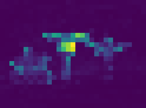
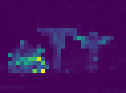
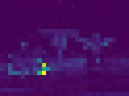
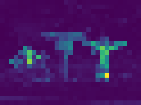
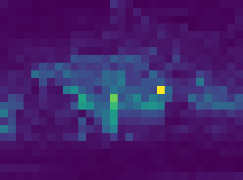
(a) CLS attention

[Patch correlation to a patch (red square) given the key feats.]

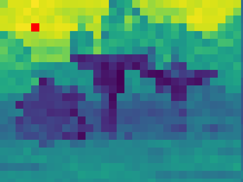
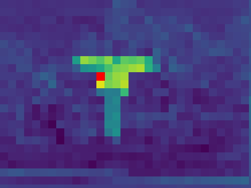
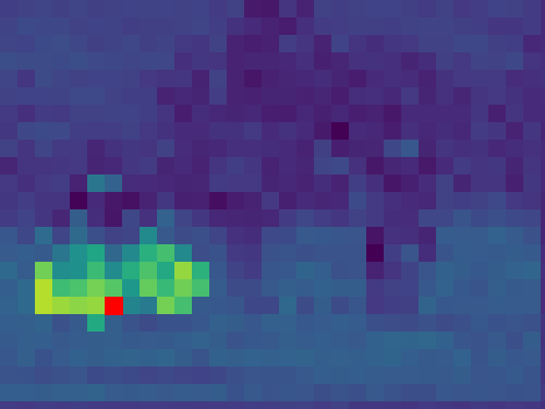
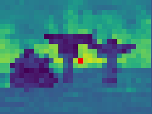
[Original image]

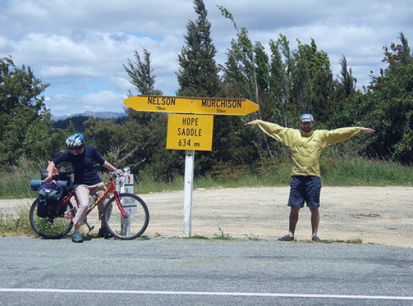
[Inverse degree (used in LOST [85])]

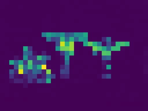
[2nd eigenvector (used in TokenCut [111])]

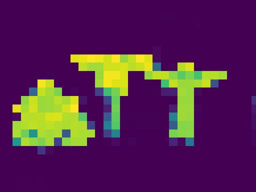
Figure 4: Object localization using DINO’s last attention layer. Visualization of different features extracted from the last attention layer of DINO [16] for the original image (c): (a) CLS attention maps generated with all heads; (b) Correlation between a patch of interest (in red) and all other patches given the key features of the last MSA layer; (d-e) Inverse degree matrix and second eigenvector, which are used to extract finer localization information [85, 111] (more details in Sec. 3.3.2, 3.3.3).

3.2 Self-supervised features

Alongside the developments of ViTs, self-supervised training strategies [16, 40, 128, 6, 22] have successfully been designed to learn useful representations without any manual annotation. Interestingly, Caron et al. [16] have shown that ViTs pre-trained in a self-supervised manner exhibit strong localization properties which contrast with those of models trained using fully supervised methods for image classification. We visualize in 4(a) the attention maps of the CLS token of each head and observe that foreground objects indeed receive most of the attention.

Although the localization properties of the attention of DINO [16] are visually enticing, they hardly suffice to directly localize objects. Indeed, different heads of the ViT model focus on different objects and regions of the image. Moreover, complex scenes have noisier attention [85]. Therefore, it is not obvious what is object or not.

A possible strategy to extract object localization information from the CLS attention maps consists in choosing the map of the best head, binarize it and get the connected components. The choice of the attention head can be fixed based on dataset performance or determined dynamically per image using heuristics, e.g. selecting the head producing the mask with the highest average IoU overlap with other heads’ outputs. We refer to this strategy as ‘DINO’ in tables. Although this approach is straight-forward, it does not fully exploit the potential of the pre-trained ViT as shown in [85]. Amir et al. [2] also reveal that self-supervised features have a rich semantic space which allows them to easily find object parts shared amongst different semantically close objects, for instance animals.

Moving the focus from the attention maps to the features of the last MSA layer, different works [85, 111, 108] have shown that in particular the key features have very good correlation properties (as visible in Fig. 4) and propose simple strategies to extract objects, which we describe now.

3.3 Training-free single-object localization with ViT self-supervised features

In this section, we discuss some of the latest unsupervised methods for locating a single object in an image. One way to do so is to apply directly $k$-means on self-supervised features [58], or to project such features on their first component after PCA analysis and use a simple threshold to separate objects and background [61]. We rather concentrate here on methods which leverage correlations among patches and are able to achieve high performance without needing any additional training step. Most of those methods are based on the following key observations about self-supervised features (especially those of DINO [16]): (1) features from two different patches of a same object are highly correlated; (2) features from two different background patches are highly correlated; but (3) features from an object patch and a background patch do not correlate well. As a result, when constructing a similarity graph $\mathcal{G}$ among all patches in a image, where similarity is defined as feature correlation, object and background patches naturally form distinct clusters within this graph. This explains why recent methods leverage such a graph and different ways to identify an ‘object cluster’ in $\mathcal{G}$.

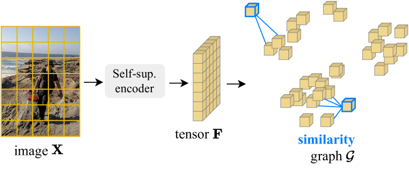
Figure 5: Feature similarity graph for unsupervised object localization. A similarity graph $\mathcal{G}$ among patches of an image is built and used by different unsupervised object localization methods [85, 111, 83, 108, 86].

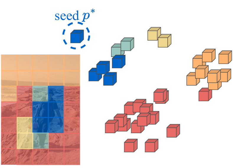
(a) LOST [85]

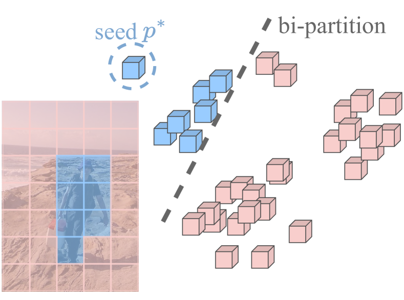
(b) TokenCut [111]

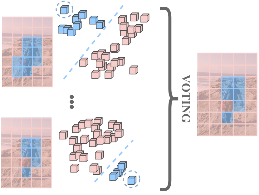
(c) SelfMask [83] coarse mask

Figure 6: Different strategies to exploit the similarity graph $\mathcal{G}$. (a) LOST [85] exploits the inverse degree information to find the seed patch $p^{*}$ (from high in blue to low in red); (b) TokenCut [111] splits the graph in two subsets given a bipartition (in blue and pink); (c) SelfMask [83] computes the partitioning on different features before voting for the most popular. Those methods are discussed in details in Sec. 3.3.2 and Sec. 3.3.3.

3.3.1 Patch-similarity graph

The graph $\mathcal{G}$ introduced before is constructed using $\ell_{2}$-normalized patch features ${\mathbf{f}_{p}\in^{d}}$ with $p\in\{1,\ldots,N\}$ the index corresponding to each patch position ($N$ is the total number of patches). Most methods below leverage ViTs and this patch feature is typically the normalized key of patch $p$ in the last attention layer–which has been shown to have the best correlation properties [85, 111]. The undirected graph of patch similarities $\mathcal{G}$ is then represented by the binary (symmetric) adjacency matrix $\mathbf{A}\,{=}\,(a_{pq})_{1\leq p,q\leq N}\in\{0,1\}^{N\times N}$ such that

$$a_{pq}=\left\{\begin{array}[]{ll}1&\text{if }\mathbf{f}_{p}^{\smash{{}^{\top}}}\mathbf{f}_{q}\geq\delta,\\ \varepsilon&\text{otherwise},\end{array}\right.$$ (4)

with $\delta\in[0,1]$ a constant threshold and $\varepsilon\geq 0$ a small value ensuring a full connectivity of the graph. In this graph, two patches $p$ and $q$ are thus connected by an undirected edge if their features $\mathbf{f}_{p}$ and $\mathbf{f}_{q}$ are sufficiently positively correlated. We review below the different ways to extract an object cluster from the graph encoded by $\mathbf{A}$.

3.3.2 Growing object clusters from selected patch seeds

Beyond the correlation properties listed above, it is possible to highlight a single cluster in $\mathcal{G}$ by exploiting the following assumption: objects often occupy less space than the background in images, hence object patches tend to have a smaller number of connection in $\mathcal{G}$ than background patches. Leveraging both assumptions, LOST [85] measures this quantity by using the degree of the nodes in $\mathcal{G}$:

$$d_{p}=\sum_{q=1}^{N}a_{pq}.$$ (5)

The patch ${p^{*}=\arg\min d_{p}}$ with the smallest degree in $\mathcal{G}$ is selected as likely corresponding to an object patch and is called the seed. We visualize the seed selection in 6(a). Then all patches connected to $p^{*}$ in $\mathcal{G}$ are considered part of the same object. Note that $\delta=\varepsilon=0$ in LOST.

Because the process above tends to miss some parts of the object, an extra step of ‘seed expansion’ is proposed in LOST. It consists in selecting the next best seeds after $p^{*}$. They are defined as the patches of small degree that are connected to $p^{*}$ in $\mathcal{G}$: ${\mathcal{S}=\{s\mid s\in\mathcal{D}_{k}\text{ and }\mathbf{f}_{s}^{{}^{\top}}\mathbf{f}_{p^{*}}\geq 0\}}$ where $\mathcal{D}_{k}$ is the set of the $k$ patches with smallest degrees, with $k$ a hyper-parameter with a typical value $k=100$. The final binary object mask $\mathbf{m}=(m_{q})_{1\leq q\leq N}$ highlights all patches that, on average, correlate positively with one of the seed patches:

$$m_{q}=\left\{\begin{array}[]{ll}1&\text{if }\sum_{s\in\mathcal{S}}\mathbf{f}_{q}^{{}^{\top}}\mathbf{f}_{s}\geq 0,\\ 0&\text{otherwise}.\end{array}\right.$$ (8)

Subsequent MaskDistill [33] employs a similar process to identify an object cluster but starts from patch seeds that are selected using the attention maps with the CLS token at the last layer of a ViT, instead of relying on the patch degree information.

3.3.3 Finer localization with different clustering methods

Bipartition using normalized graph-cut. Instead of identifying one seed in an object cluster and a cluster in which this seed belongs, TokenCut [111] and DeepSpectralMethods [63] use spectral clustering to separate objects and background. The first considers an adjacency matrix $\mathbf{A}$ computed using $\delta=0.2$ and $\varepsilon=10^{-5}$, while the second uses $\delta=\varepsilon=0$ and combines it with a nearest neighbors adjacency matrix based on color affinity. Both compute the second smallest eigenvalue and the corresponding eigenvector $\mathbf{y}^{*}$ to the generalized eigensystem

$$(\mathbf{D}-\mathbf{A})\mathbf{y}=\lambda\,\mathbf{D}\mathbf{y},$$ (9)

where $\mathbf{D}$ is the diagonal degree matrix with entries $d_{p}$ (see Eq. 5). The patches are then partitioned into two clusters $\mathcal{A}=\{p\,|\,\mathbf{y}^{*}_{p}\leq\overline{\mathbf{y}}^{*}\}$ and $\mathcal{B}=\{p\,|\,\mathbf{y}^{*}_{p}>\overline{\mathbf{y}}^{*}\}$, where $\overline{\mathbf{y}}^{*}$ is the average of the entries in $\mathbf{y}^{*}$ in [111] and $\overline{\mathbf{y}}^{*}=0$ in [63]. We visualize the bi-partition in 6(b). The cluster with the main salient object is identified as the one containing the largest absolute value $\max_{p}\left|{\mathbf{y}^{*}_{p}}\right|$ in [111], while [63] selects the smallest cluster. All patches in this cluster define the object mask $\mathbf{m}$.

$k$-partition using normalized graph-cut. Instead of relying on a single self-supervised backbone, it is possible to ensemble multiple foreground/background masks obtained from features of different self-supervised backbones. In particular, SelfMask [83] produces $k$ masks with each backbone. The authors compute the eigenvectors associated to the $k$ smallest eigenvalues in (9) (this time $a_{pq}=\mathbf{f}_{p}^{{}^{\top}}\mathbf{f}_{q}$) and gather them in $\mathbf{Y}\in\mathbb{R}^{N\times k}$. Finally, they produce the $k$ candidates by applying $k$-means on $\mathbf{Y}$. Given the mask candidates generated with the different pre-trained backbones, the most popular mask $\mathbf{m}$ is selected as the one with the highest average pairwise IoU with respect to all the other mask candidates. It is to be noted that before choosing $\mathbf{m}$ the authors try and filter out likely wrong masks, e.g. with height (resp. width) as large as the original image height (resp. width). We visualize SelMask process in 6(c).

3.4 From single- to multi-object localization

Methods described so far are limited to the discovery of one object. Recent methods, like [107, 86, 108], address this limitation and are able to discover multiple objects in one image. We first focus on the problem of foreground/background separation, before discussing means to separate objects in distinct masks.

3.4.1 objects := not(background)

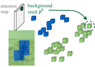
Figure 7: Background discovery in FOUND [86]. Patches that are highly correlated to the background seed patch $p^{b}$ (the one receiving the least attention in the CLS attention maps) are identified as background. See Sec. 3.4.1 for details.

Instead of constructing a method that specifically searches for a subset of the objects in the image, the authors of FOUND [86] propose to look at the problem the other way around and identify all background patches, hence discovering all object patches as a by-product with no need for a prior knowledge of the number of objects or their relative size with respect to the background. The strategy, named ‘FOUND-coarse’, starts by identifying the patch that receives the least attention with the CLS token in the last layer of a DINO-pre-trained ViT. This patch is called the background seed and its index denoted by $b$. Then the background mask $\mathbf{m}^{\rm bck}$ (visualized in Fig. 7) has entries $m_{p}^{\rm bck}$, $p=1,\ldots,N$, satisfying

$$m_{p}^{\rm bck}=\left\{\begin{array}[]{ll}1&\text{if }\mathbf{f}_{p}^{{}^{\top}}\mathbf{f}_{b}\geq\tau,\\ 0&\text{otherwise}.\end{array}\right.$$ (12)

In practice, the patch features $\mathbf{f}_{p}$ are made of the $\ell_{2}$-normalized keys at the last attention layer and $\tau=0.3$. Note that, for conciseness, we omitted the fact that an adaptive re-weighting technique is applied to the entries of $\mathbf{f}_{p}$ and $\mathbf{f}_{b}$ in (12). This re-weighting takes into account the fact that the background appears more or less clearly depending on the attention heads. Finally, the object mask $\mathbf{m}$ is the complement of $\mathbf{m}^{\rm bck}$.

3.4.2 Iterative clustering

We now discuss different solutions to directly separate the objects within the self-supervised features.

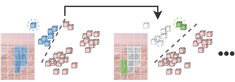
Figure 8: Iterative selection in MaskCut [108]. Object patches are iteratively selected in $\mathcal{G}$.

In an attempt to adapt TokenCut [111] to multi-objects localization, Wang et al. [108] propose to compute the first mask $\mathbf{m}$ and disconnect the corresponding patches in the graph $\mathcal{G}$ before re-applying spectral clustering to discover a second object. This simple process, named MaskCut and visualized in Fig. 8, is repeated a pre-determined number of times (3 in practice), allowing the discovery of a few well localized objects. Also, rather than strictly disconnecting the patches of $\mathbf{m}$ in $\mathcal{G}$, the authors set a small edges weight $a_{pq}=\varepsilon$ if $\mathbf{m}_{p}=1$ or $\mathbf{m}_{q}=1$ and then compute the second eigenvector of the system (9) one more time.

Similarly, UMOD [46] also builds upon TokenCut. It computes the eigenvectors associated to the $k$ smallest eigenvalues of the system (9). These eigenvectors can be gathered in a matrix $\mathbf{Y}\in\mathbb{R}^{N\times k}$ and the masks are obtained by applying $k$-means on the rows of $\mathbf{Y}$, as in SelfMask [83]. The background cluster is identified as the one covering the largest area in the image, as assumed in LOST [85], while the remaining clusters represent ‘object areas’. Distinct from CutLER, UMOD [46] dynamically determines the optimal number of clusters using an iterative process. Practically, the number of clusters is incremented from 2 until the relative change in total object area gets below a predefined threshold.

3.4.3 Analysis of correlation maps with Entropy-based Box Analysis

Alternatively, MOST [70] exploits the correlation maps between the patch features. The authors notice that such maps are sparser when computed using an object patch as reference than when using a background patch. Thus they propose to analyze all these maps to determine a set of patches likely to fall on objects. The correlation maps are processed with an Entropy-based Box Analysis (EBA) method which discriminates the correlation maps based on their entropy (measured at multiple scales). The patches that yield the correlation maps with lowest entropy (likely to be object patches) are clustered providing different pools. One object mask is then created from each of these pools with a process similar to LOST [85]: (1) the patches of the lowest degree in $\mathcal{G}$ in the current pool are extracted, playing the role of the seed (called core in [70]); (2) all patches in the current pool negatively correlated with the seed are filtered out; (3) the mask is then made of all patches positively correlated with the patches left in the pool. This three-step process is repeated for each pool, hence discovering multiple objects.

3.4.4 Different queries for different objects

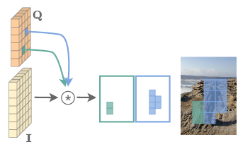
Figure 9: Generation of several potential masks in FreeMask [107]. As many masks are produced as there are patches in $\mathbf{Q}$, tensors $\mathbf{Q}$ and $\mathbf{I}$ being features extracted from a ResNet50 pre-trained with self-supervised denseCL [106].

Leveraging pixel-level similarity, FreeMask [107] exploits this time convolutional neural networks – a ResNet50 [38] pre-trained with self-supervised denseCL [106]; Its principle is illustrated in Fig. 9. The features $\mathbf{I}\in^{H\times W\times d}$, generated for the image $\mathbf{X}$, are down-sampled into features $\mathbf{Q}\in^{H^{\prime}\times W^{\prime}\times d}$ with reduced sizes $H^{\prime}$ and $W^{\prime}$. The downsampled features $\mathbf{Q}$ are reshaped to matrix of size $N^{\prime}\times d$ where $N^{\prime}=H^{\prime}W^{\prime}$. We denote by $\mathbf{Q}_{q}\in\mathbb{R}^{d}$ the features at spatial position $q$ in $\mathbf{Q}$. Each $\mathbf{Q}_{q}$ is then considered as a seed and compared to all pixels in $\mathbf{I}$ producing a soft map $\mathbf{s}\in^{H\times W\times N^{\prime}}$ with entries

$$s_{i,j,q}=\frac{\mathbf{Q}_{q}^{{}^{\top}}\mathbf{I}_{i,j}}{\|\mathbf{Q}_{q}\|\|\mathbf{I}_{i,j}\|},$$ (13)

which is normalized to range in $[0,1]$. This soft map is then binarized to obtain $\mathbf{m}\in^{H\times W\times N^{\prime}}$ with entries

$$m_{i,j,q}=\left\{\begin{array}[]{ll}1&\text{if }s_{i,j,q}>\tau,\\ 0&\text{otherwise},\end{array}\right.$$ (16)

with $\tau\!\in\,(0,1]$ a hyperparameter. These $N^{\prime}$ masks of spatial size $H\times W$ in $\mathbf{m}$ are then sorted based on an objectness score and “the best” ones are selected using an NMS-like function. In addition, different scales are used to produce more queries.

3.5 Post-processing

To adapt the produced masks to the final downstream task, it is possible to leverage different post-processing methods. We first discuss in Sec. 3.5.1 ways to improve the quality of generated masks by using pixel-level information. Second, in the case of object discovery/detection, we briefly discuss in Sec. 3.5.2 how to generate boxes given the generated masks.

3.5.1 Pixel-level refinement

In order to further improve the quality of the produced masks, popular refinement strategies [10, 52] have been successfully applied to fit masks to pixel-level information. Indeed Bilateral Solver (BS) [10] and Conditional Random Field (CRF) [52] use the raw pixel color and positional information in order to refine the generated coarse masks. Requiring no specific training, it is to be noted that the application of such methods can be expensive and sometime hurts the quality of the mask as discussed in [12, 86].

Alternatively, recent PaintSeg [57] introduces a training-free model to estimate precise object foreground-background masks from either a bounding box or a predicted coarse mask. The method iteratively refines masks by in-painting the foreground and out-painting the background, updating masks through image comparisons. In-painting uses a pre-trained diffusion generative model [74], while for image comparison employs a pre-trained DINO model [16]. Such method generates high quality masks and obtains very good results as discussed in Sec. 3.6.

3.5.2 From mask to box

In order to produce bounding boxes given a localization mask, e.g. for the task of unsupervised detection, methods separate the mask in connected components and enclose each of them with the tightest box. In the case of unsupervised object discovery, they produce a tight box only for the biggest component [86, 83] or the one including the object seed $p^{*}$ [85, 111].

		DUT-OMRON [120]			DUTS-TE [102]			ECSSD [82]			CUB [101]
Method	post-proc.	Acc	IoU	max $F_{\beta}$	Acc	IoU	max $F_{\beta}$	Acc	IoU	max $F_{\beta}$	Acc	IoU	max $F_{\beta}$
—SoTA before self-supervised ViTs era—
E-BigBiGAN [100]		86.0	46.4	56.3	88.2	51.1	62.4	90.6	68.4	79.7	—	—	—
Melas-Kyriazi et al. [62]		88.3	50.9	—	89.3	52.8	-	91.5	71.3	—	—	—	—
—Without post-processing—
SelfMask (coarse) [83]		81.1	40.3	—	84.5	46.6	—	89.3	64.6	—	—	—	—
LOST [85]		79.7	41.0	47.3	87.1	51.8	61.1	89.5	65.4	75.8	95.2	68.8	78.9
DSM [63]		80.8	42.8	55.3	84.1	47.1	62.1	86.4	64.5	78.5	94.1	66.7	82.9
MOST [70]		87.0	47.5	57.0	89.7	53.8	66.6	89.0	63.1	79.1	—	—	—
FOUND-coarse [86]		—	—	—	—	—	—	90.6	70.9	78.0	—	—	—
TokenCut [111]		88.0	53.3	60.0	90.3	57.6	67.2	91.8	71.2	80.3	96.4	74.8	82.1
—With post-processing—
LOST [85]	BS	81.8	48.9	57.8	88.7	57.2	69.7	91.6	72.3	83.7	96.6	77.6	84.3
DSM [63]	CRF	87.1	56.7	64.4	83.8	51.4	56.7	89.1	73.3	80.5	96..6	76.9	84.3
FOUND-coarse [86]	BS	—	—	—	—	—	—	90.9	71.7	79.2	—	—	—
TokenCut [111]	BS	89.7	61.8	69.7	91.4	62.4	75.5	93.4	77.2	87.4	97.4	79.5	87.1
PaintSeg (on TokenCut)[57]	yes	—	—	—	—	67.0	—	—	80.6	—	—	—	—

Table 3: Evaluation of unsupervised saliency detection methods. Comparisons of methods solely leveraging pre-trained self-supervised features (discussed in Sec. 3). The task is described in Sec. 2.2. We separate in two section results of methods with and without post-processing. We produce the two best previous baselines in the ‘previous SoTA section’, more are provided in Tab. 6.

3.6 Quantitative results

We quantitatively compare the methods presented in this section, utilizing reported results from various papers. Specifically, in Sec. 3.6.1, we discuss methods for unsupervised object discovery, while in Sec. 3.6.2, we focus on methods dedicated to unsupervised saliency detection. The comparison of class-agnostic multi-object detection or segmentation methods is deferred for subsequent discussion (Sec. 4.5).

Method	VOC07 [31]	VOC12 [32]	COCO 20k [59, 97]
—SoTA before self-supervised ViTs era—
LOD [98]	53.6	55.1	48.5
rOSD [95]	54.5	55.3	48.5
—Leveraging self-supervised features—
DINO [16]	45.8	46.2	42.1
LOST [85]	61.9	64.0	50.7
DSS [63]	62.7	66.4	52.2
TokenCut [111]	68.8	72.1	58.8

Table 4: Single-object discovery. Results for the methods described in Sec. 3. The task is described in Sec. 2.3 and evaluated with the Correct Localization (CorLoc) metric. We produce the two best previous baselines in the ‘previous SoTA section’, more are provided in Tab. 7.

3.6.1 Single-object discovery

The capability of methods to perform single-object discovery is typically evaluated using the CorLoc metric as detailed in Sec. 2.3. We report in Tab. 4 CorLoc results on the datasets VOC07 [31], VOC12 [32], COCO20k [59]. We report best results of each method obtained with the backbone model ViT-S/16 pre-trained following DINO [16]. If interested, authors of TokenCut produce an interesting table (Tab. 5 in their paper) to compare different backbones.

We observe that LOST [85], TokenCut [111] and Deep Spectral Methods [63] (noted DSS in the table) largely surpass previous baselines, and thus without performing dataset-level optimization. Also TokenCut obtains best results and produces a good prediction in $\approx 70\%$ of the time on both VOC07 and VOC12. In the more challenging dataset COCO, methods are still able to predict an accurate box half of the time. It is to be noted that TokenCut and DSS both require to compute eigenvectors which has some computational cost.

3.6.2 Unsupervised saliency detection

The quality of the multi-object localization can be measured using the unsupervised saliency detection protocol (detailed in Sec. 2.2) which evaluates how well the foreground pixels are separated from the background ones. We report results provided by the authors or following works in Tab. 3.

Comparison of methods. We first focus on the results of the methods without the application of post-processing. We can observe that best results are obtained by TokenCut [111] again on all datasets. Results of LOST and DSS are on par with one another, DSS being better on DUT-OMRON and LOST better on other datasets. It is to be noted that methods noted with ‘coarse’ are not the final results of the methods and are further improved by using training strategies discussed in Sec. 4. Also, MOST [70] is not designed directly for the task of unsupervised saliency detection; in order to produce a score the authors select the largest pool and use as saliency map the similarity map computed using its tokens.

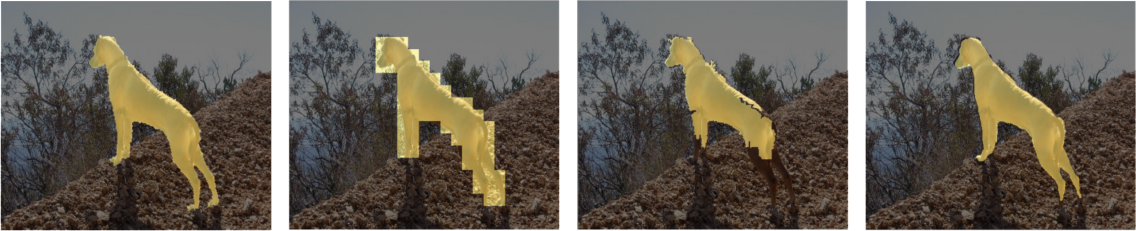
louuu GT louuu TC [111] looou TC+BS louu PaintSeg [57]

Figure 10: Visualization of the impact of the post-processing. We observe improvements on the borders of the mask with the application of Bilateral Solver (BS) [10] and PaintSeg [57] on the results of TokenCut [111], noted ‘TC’. The figure is borrowed from PaintSeg [57].

Post-processing refinement. We now discuss the impact of the post-processing step and observe that in all cases, results are significantly boosted. For instance LOST, DSM and TokenCut are all boosted by around 8 pts of IoU on DUT-OMRON showing the importance and opportunity provided by post-processing to refine masks. Moreover, by employing the latest post-processing strategy, PaintSeg [57], the results of TokenCut are further improved. We present the visual results of TokenCut with the Bilateral Solver (BS) and PaintSeg in Fig. 10; we observe that while the Bilateral Solver (BS) refines the mask, it concurrently introduces degradation, observed on the leg of the dog—–an acknowledged phenomenon reported in previous studies [86]. In contrast, the output of PaintSeg aligns more closely with the ground truth.

3.7 Limits

Leveraging self-supervised features of transformers allow us to discover objects with no annotation and achieve interesting single-object discovery performances on VOC and COCO datasets. However, extending this capability to multi-object discovery is not straight-forward and several questions remain on how to:

• successfully perform multi-object detection?

• exchange information at a dataset level?

• refine results?

We examine in the next section how integrating a simple learning step can greatly boost results and generalisability properties.

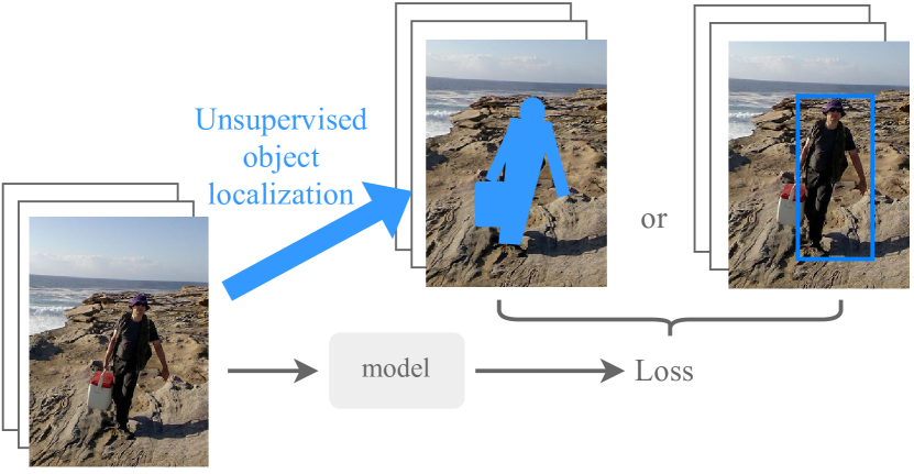
Figure 11: Improving through learning. Leveraging the coarse discovered objects to learn powerful models for downstream tasks.

4 Improving through learning

All methods presented so far are designed to extract as much as information as possible from features of an already pre-trained backbone. Solutions to improve the performance consists in leveraging the available data for the task of interest and tailoring the self-supervised features by adding a learnable head on top of them, learning a new model specific to the downstream task, or actually finetuning the self-supervised features to improve their localization properties (without using ground-truth annotations). Up to few exceptions, the methods discussed below use masks or boxes discovered by the previously-discussed methods as pseudo-labels.

4.1 Unsupervised foreground segmentation

For the task of unsupervised foreground segmentation, most of the methods exploit frozen DINO features and train a segmentation head to tailor these features to the task.

4.1.1 Tailoring DINO features

Linear separation of the features. One of the simplest ways to tailor DINO features is probably to add a single 1x1 convolution layer on top of them [86]. The method FOUND [86] learns to project the self-supervised features to an ‘objectness’ space and is trained using two objectives: the first guides the prediction towards the coarse masks of Sec. 3.4.1; the second guides the predictions towards its own post-processed version. Specifically, the authors use as post-processing the Bilateral Solver operation which improves the quality of the masks and is discussed in Sec. 3.5. This work shows that foreground and background patches are linearly separable in the feature space of a DINO-pre-trained ViT. Song et al. [87] also employ a linear layer trained on frozen self-supervised pre-trained patch features but using the Representer Point Selection [122] framework. They utilize soft pseudo-masks derived from the magnitude of these pre-trained features as foreground-background target masks: higher feature magnitudes in patches indicate the presence of a salient object.

Towards higher-resolution predictions. Alternatively, SEMPART [71] incorporates a transformer layer, followed by a 1x1 convolution layer with a sigmoid activation unit on top of the fixed DINO features. The training objective minimizes the normalized cut loss across a graph defined by an adjacency matrix as defined in (4). In other words, SEMPART is crafted to learn to predict the (soft) bi-partition of a graph that has similar properties as the one used in, e.g., LOST or TokenCut (see Sec. 3.3). As the mask at the output of this first step is defined at patch-level and is thus coarse, SEMPART jointly trains an upconvolution network to refine the prediction. This network processes and complements the features extracted from the transformer layer with RGB features at progressively increasing resolutions, resulting in a finer mask at the original image resolution. The training process for these refined masks involves a coarse-to-fine mask distillation process wherein the finer masks, after being downsampled through average pooling, are required to match the coarse masks. Furthermore, SEMPART smooths the predictions and ensures the preservation of fine boundary details through the incorporation of graph-driven total-variation regularization losses. In summary, instead of partitioning a graph to obtain a first mask and improving the quality of this mask by post-processing, SEMPART is able to learn this full process end-to-end by making each step differentiable. Let us mention that DeepCut [1] also exploits the idea of minimizing the normalized cut loss (or some variation) to train a lightweight graph neural network on top of frozen DINO features.

Learning by moving objects. MOVE [12] exploits two self-supervised ViTs: the first with DINO; the second with MAE. A segmentation head is trained on top of the frozen DINO features with the help of the MAE-pre-trained ViT. The training objective is constructed on the fact that if objects are accurately segmented and the background inpainted using the pre-trained MAE, then the objects can be pasted at a different location in the image without generating duplication artifacts. The segmentation head is trained using an adversarial loss design to detect these duplication artifacts. The concept that foreground objects can be “realistically moved” within an image or to other images has also been investigated in [72, 67, 11, 5, 121, 76, 48].

Leveraging low-level information. The idea of modifying DINO features is also exploited in UCOS-DA [126] to address the problem of the discovery of camouflaged objects, i.e., when objects and background share similar colors and textures. UCOS-DA [126] also trains an additional head on top of a frozen DINO encoder using pseudo-masks generated by a training-free foreground/background discovery method. It also incorporates a foreground-background contrastive objective to improve the performance on this task.

4.1.2 Training new networks

Unlike the former methods, SelfMask [83] does not tailor frozen self-supervised features but trains a dedicated segmenter network (a variant of MaskFormer [24]) supervised using the pseudo-masks generated as in Sec. 3.3.3. This training phase leads to masks of higher quality than the pseudo-masks.

Let us mention that the authors of MOVE also train a MaskFormer with the training protocol of SelfMask but using the masks they obtained with the method described just above in Sec. 4.1.1.

4.2 Class-agnostic multi-object detection

In order to go from single-object discovery to multiple object detection, the authors of LOST [85] propose to train a class-agnostic detection (CAD) model. They train a classic object detection model, namely Faster R-CNN [73], and use the boxes produced in Sec. 3.3.2 as pseudo-labels. But given the lack of knowledge about object classes, the authors propose to adapt the training by assigning the single class ‘object’ to all pseudo-boxes and do not modify the Faster R-CNN architecture. Such training regularizes the boxes through the dataset and overall improves their quality, as seen with the improvement of the CorLoc scores shown in Tab. 5. Additionally, the model predicts several boxes per image even if trained with a single pseudo-box per image. This class-agnostic strategy has been adopted by different single-object discovery methods [111, 12] and all show the benefit of the training to obtain more and better boxes.

In an attempt to further augment the number of boxes produced per image, CutLer [108] proposes to re-train a detection model (this time a Mask R-CNN [39]) several times, each round using the coarse boxes or the prediction of the previous training. In practice, they perform three such rounds and show that the number of produced detections increases after each round. We discuss this method in greater details in Sec. 4.3.

Method	+ CAD	VOC07	VOC12	COCO20k
LOST [85]		61.9	64.0	50.7
	✓	65.7 +3.8	70.4 +6.4	57.5 +6.8
TokenCut [111]		68.8	72.1	58.8
	✓	71.4 +2.6	75.3 +3.2	62.6 +3.8
MOVE [12]		76.0	78.8	66.6
	✓	77.1	80.3	69.1

Table 5: Multi-object discovery with class-agnostic detection. Results using the ‘+CAD’ strategy on the VOC and COCO datasets for different self-supervised feature extraction methods [85, 111, 12] highlighted in the table. Evaluation with the CorLoc metric.

4.3 Class-agnostic instance segmentation

Moving forward towards the finer task of unsupervised instance segmentation, the methods [107, 108, 44, 58] propose to train an instance segmentation model which generates a mask per object instance. All of them use coarse masks as pseudo-labels.

Learning an instance segmentation model. First, FreeSOLO [107] utilizes the pseudo instance-masks, generated thanks to the FreeMask methodology (detailed in Sec. 3.4.4), for training a SOLO-based [104] instance segmentation model. To enhance stability in the presence of inherently noisy pseudo-masks, FreeSOLO introduces modifications to the training protocol of SOLO. Drawing inspiration from the weakly-supervised literature, they project SOLO-predicted instance masks and pseudo masks onto the x and y axes, enforcing alignment through a corresponding loss. At the same time, FreeSOLO incorporates a pairwise affinity loss leveraging the expectation that proximal pixels with similar color should share the same class in predicted masks (foreground or background class). In the absence of semantic classes, SOLO predicts an objectness score and a semantic embedding for each instance, extracted from pre-trained features. To further improve accuracy, FreeSOLO employs self-training, leveraging the initially trained SOLO-based instance segmenter.

Subsequent exemplar-FreeSOLO [44] enhances FreeSOLO by introducing an unsupervised mechanism for generating object exemplars which can be seen as a vocabulary. Leveraging these exemplars, the model extracts pseudo-positive/negative objects for each image, enabling the formulation of a contrastive loss. This loss enhances the discriminative capability of the SOLO-based instance segmenter, leading to better results.

Alternatively, both CutLer [108] and IMST [58] train a class-agnostic Mask R-CNN [39] instance segmentation model. Both use pseudo labels generated from the self-supervised features. CutLer model is trained with initial coarse instance masks generated for each image via their MaskCut methodology (detailed in Sec. 3.4.2). They also enhance Mask R-CNN learning by employing a loss dropping strategy which excludes regions with no IoU overlap with any pseudo-mask. This strategy boosts robustness to objects overlooked by MaskCut. Additionally, they further improve the instance segmentation model using multiple rounds of self-training.

Learning to denoise and merge object parts with classifiers. We have seen in Sec. 3.4.2 that UMOD [46] leverages iterative clustering with a stopping criterion which allows the estimation of the number of objects in an image. This process is nevertheless imperfect resulting in discovery of object parts rather than complete objects. The authors therefore post-process the masks by merging object parts using two convolutional classifiers trained with the help of automatically extracted pseudo-labels. The first is trained to distinguish foreground/object parts from background parts. The second applies on foreground parts to assign them a pseudo-class representing semantic concepts discovered at the level of the dataset.

	DUT-OMRON [120]			DUTS-TE [102]			ECSSD [82]			CUB [101]
Method	Acc	IoU	max $F_{\beta}$	Acc	IoU	max $F_{\beta}$	Acc	IoU	max $F_{\beta}$	Acc	IoU	max $F_{\beta}$
—SoTA before self-supervised ViTs era—
HS [119]	84.3	43.3	56.1	82.6	36.9	50.4	84.7	50.8	67.3	—	—	—
wCtr [130]	83.8	41.6	54.1	83.5	39.2	52.2	86.2	51.7	68.4	—	—	—
WSC [56]	86.5	38.7	52.3	86.2	38.4	52.8	85.2	49.8	68.3	—	—	—
DeepUSPS [65]	77.9	30.5	41.4	77.3	30.5	42.5	79.5	44.0	58.4	—	—	—
BigBiGAN [100]	85.6	45.3	54.9	87.8	49.8	60.8	89.9	67.2	78.2	—	—	—
E-BigBiGAN [100]	86.0	46.4	56.3	88.2	51.1	62.4	90.6	68.4	79.7	—	—	—
Melas-Kyriazi et al. [62]	88.3	50.9	—	89.3	52.8	-	91.5	71.3	—	—	—	—
—Without post-processing—
MOST [70]	87.0	47.5	57.0	89.7	53.8	66.6	89.0	63.1	79.1	—	—	—
WSCUOD [61]	89.7	53.6	64.4	91.7	89.9	73.1	92.2	72.7	85.4	96.8	77.8	87.9
FreeSOLO [107]	90.9	56.0	68.4	92.4	61.3	75.0	91.7	70.3	85.8	—	—	—
LOST [85]	79.7	41.0	47.3	87.1	51.8	61.1	89.5	65.4	75.8	95.2	68.8	78.9
DSM [63]	80.8	42.8	55.3	84.1	47.1	62.1	86.4	64.5	78.5	94.1	66.7	82.9
TokenCut [111]	88.0	53.3	60.0	90.3	57.6	67.2	91.8	71.2	80.3	96.4	74.8	82.1
DeepCut: CC loss [1]	—	—	—	—	56.0	—	—	73.4	—	—	77.7	—
DeepCut: N-cut loss [1]	—	—	—	—	59.5	—	—	74.6	—	—	78.2	—
SelfMask [83]	90.1	58.2	—	92.3	62.6	—	94.4	78.1	—	—	—	—
FOUND [86]-single	92.0	58.6	67.3	93.9	63.7	73.3	91.2	79.3	94.6	—	—	—
FOUND-multi [86]	91.2	57.8	66.3	93.8	64.5	91.5	94.9	80.7	95.5	—	—	—
MOVE [12]	92.3	61.5	71.2	95.0	71.3	81.5	95.4	83.0	91.6	—	85.8	—
UCOS-DA [126]	—	—	—	—	—	—	95.1	81.6	89.1	—	—	—
SEMPART-fine [71]	93.2	66.8	76.4	95.9	74.9	86.7	96.4	85.5	94.7	—	—	—
SelfMask [83] on MOVE [12] [71]	93.3	66.6	75.6	95.4	72.8	82.9	95.6	83.5	92.1	—	—	—
SelfMask [83] on SEMPART-fine [71]	94.2	69.8	79.9	95.8	74.9	87.9	96.3	85.0	94.4	—	—	—
—With post-processing—
LOST [85] + BS	81.8	48.9	57.8	88.7	57.2	69.7	91.6	72.3	83.7	96.6	77.6	84.3
DSM [63] + CRF	87.1	56.7	64.4	83.8	51.4	56.7	89.1	73.3	80.5	96.6	76.9	84.3
WSCUOD [61] + BS	90.9	58.5	68.3	92.5	63.0	76.4	92.8	74.2	89.6	97.3	79.7	89.3
TokenCut [111] + BS	89.7	61.8	69.7	91.4	62.4	75.5	93.4	77.2	87.4	97.4	79.5	87.1
FOUND-single [86] + BS	92.1	60.8	70.6	94.1	64.5	76.0	94.9	80.5	93.4	—	—	—
FOUND-multi [86] + BS	92.2	61.3	70.8	94.2	66.3	76.3	95.1	81.3	93.5	—	—	—
SelfMask [83] + BS	91.9	65.5	—	93.3	66.0	—	95.5	81.8	—	—	—	—
PaintSeg (on TokenCut)[57]	—	—	—	—	67.0	—	—	80.6	—	—	—	—
MOVE [12] + BS	93.1	63.6	73.4	95.1	68.7	82.1	95.3	80.1	91.6	—	—	—
SelfMask [83] on MOVE [12] + BS [71]	93.7	66.5	76.6	95.2	68.7	82.7	95.2	80.0	91.7	—	—	—

Table 6: Unsupervised saliency detection evaluation. We reproduce here published results on the task described in Sec. 2.2. We note with a green citation in which paper the score was found (if not from the original paper). We produce results with and without a post-processing step in different table sections. We note the application of a post-processing step with ‘+BS’ (Bilateral Solver [10]), ‘+CRF’ ( [52]) and PaintSeg [57] is a post-processing strategy.

4.4 Going further by finetuning DINO-ViT backbones

While this section was structured so far based on the main task addressed by each method, we change focus here. We now discuss methods that finetune directly DINO-pre-trained ViT backbones without loosing any of their object localization properties, and actually improving them for the tasks of interest.

Learning scene-centric features. Following classic self-supervised setup, DINO backbones [16] are trained on object-centric images from ImageNet [28] and Lv et al. [61] observe that DINO features are noisy on natural scene-centric images and struggle on complex (e.g., cluttered) background. A promising solution, explored in WSCUOD [61] is to finetune the self-supervised features on scene-centric images, e.g., DUTS [102]. In order to guide the finetuning on such images and encourage the suppression of the background activation, the authors propose two strategies. The first is a weakly-supervised contrastive learning (WCL) [127] to explore inter-image semantic relationships. WCL assigns weak labels to images based on graph-based similarity and then enhances image similarity through supervised contrastive learning. The second is a pixel-level semantic alignment loss [117] that encourages the pixel-level consistency of the same object across different views of the same image.

Detect to finetune features. The authors of [34] propose to refine self-supervised features for the task of single-object discovery by: (1) training a detection head directly applied on top of a frozen self-supervised backbone, (2) freezing this detection head and (3) finetuning the self-supervised backbone. The detection head is trained using boxes extracted, e.g., using LOST, TokenCut or MOVE. Once this detection head is trained, a fixed number of boxes is extracted per image to serve as supervision signal to finetune the self-supervised backbone. During finetuning, a regularisation term is also added on the output features of the self-supervised backbone to prevent it to diverge too far from its original state. The newly finetuned features can then be re-used in, e.g., LOST, TokenCut, or MOVE for single-object discovery (see Tab. 7).

Method	VOC07	VOC12	COCO 20k
—SoTA before self-supervised ViTs era—
Selective Search [90]	18.8	20.9	16.0
EdgeBoxes [132]	31.1	31.6	28.8
Kim et al. [50]	43.9	46.4	35.1
Zhang et al. [124]	46.2	50.5	34.8
DDT+ [113]	50.2	53.1	38.2
rOSD [96]	54.5	55.3	48.5
LOD [98]	53.6	55.1	48.5
—No learning—
DINO [16]	45.8	46.2	42.1
LOST [85]	61.9	64.0	50.7
DSS [63]	62.7	66.4	52.2
TokenCut [111]	68.8	72.1	58.8
—With learning—
FreeSOLO [107][12]	56.1	56.7	52.8
LOST [85] + CAD	65.7	70.4	57.5
DeepCut: CC loss [1]	68.8	67.9	57.6
DeepCut: N-cut loss [1]	69.8	72.2	61.6
WSCUOD [61]	70.6	72.1	63.5
TokenCut [111] + CAD	71.4	75.3	62.6
SelfMask [83]	72.3	75.3	62.7
FOUND [86]	72.5	76.1	62.9
SEMPART-Coarse [71]	74.7	77.4	66.9
SEMPART-Fine [71]	75.1	76.8	66.4
IMST [58]	76.9	78.7	72.2
MOVE [12]	76.0	78.8	66.6
MOVE [12] + CAD	77.1	80.3	69.1
MOVE multi [12] + CAD	77.5	81.5	71.9
Bb refin. [34] w. MOVE	77.5	79.6	67.2
Bb refin. [34] w. MOVE + CAD	78.7	81.3	69.3

Table 7: Single-object discovery. The task is described in Sec. 2.3 and evaluated with the Correct Localation (CorLoc) metric on the datasets VOC07 [31], VOC12 [32] and COCO 20k [59, 97]. If the score was not reported in the original paper, we cite in green the paper which produced it.

		COCO 20K [59, 96]					PASCAL VOC07 [31]					PASCAL VOC12 [32]			COCO val2017 [59]
Method	Detector	AP50	AP75	AP	odAP50	odAP	AP50	AP75	AP	odAP50	odAP	AP50	odAP50	odAP	AP50	AP75	AP
—No learning—
rOSD [95]			—	—	5.2	1.6		—	—	13.1	4.3	—	15.4	5.27	—	—	—
LOD [98]			—	—	6.6	2.0		—	—	13.9	4.5	—	16.1	5.34	—	—	—
TokenCut [111]	—	—	—	—	—	—	—	—	—	—	—	—	—	—	5.8	2.8	3.0
MOST [70]	—					1.7					6.4
—With learning—
rOSD [95] + CAD	FRCNN	8.4	—	—	—	—	24.2	—	—	—	—	29.0	—	—	—	—	—
LOD [98] + CAD	FRCNN	8.8	—	—	7.3	2.3	22.7	—	—	15.8	5.0	28.4	20.9	7.07	—	—	—
LOST [85] + CAD	FRCNN	9.9	—	—	7.9	2.5	29	—	—	19.8	6.7	33.5	24.9	8.85	—	—	—
TokenCut [111] + CAD	FRCNN	10.5	—	—	—	—	26.2			—	—	35.0	—	—	—	—
UMOD [46]	ResNet50	13.8	—	—	5.4	2.1	27.9	—	—	15.4	6.8	36.2		—	—	—	—
FreeSOLO [107]	SOLO	12.4	4.4	5.6	—	—	24.5	7.2	10.2	—	—	—	—	—	12.2	4.2	5.5
Ex.-FreeSOLO [44]	SOLO	—	—	—	—	—	26.8	8.2	12.6	—	—	—	—	—	17.9	8.6	12.6
WSCUOD [61]	FRCNN	13.6	—	—	—	—	30.5	—	—	—	—	—	—	—	—	—	—
IMST [58]	MRCNN	—	—	—	—	—	—	—	—	—	—	—	—	—	18.1	7.6	8.8
MOVE [12]			—	—	—	—	—	—	—	—	—	—	—	—	19	6.5	8.2
CutLER [108]	MRCNN	21.8	11.1	10.1	—	—	—	—	—	—	—	—	—	—	21.3	11.1	10.2
CutLER [108]	C-MRCNN	22.4	12.5	11.9	—	—	36.9	19.2	20.2	—	—	—	—	—	21.9	11.8	12.3

Table 8: Class-agnostic multi-object detection. The task and metrics are described in Sec. 2.4. The task is described Sec. 2.4. We note the detector model used in the column ‘Detector’: ‘FRCNN’ stands for Faster R-CNN [73], ‘MRCNN’ for Mask R-CNN [39], ‘C-MRCNN’ for Cascade Mask R-CNN [13] and SOLO model is described in [104]. UMOD learns two classifiers which are based on a ResNet50 [38] backbone. Notation ‘+CAD’ denote training a Faster R-CNN [73] following [85].

		COCO 20K [59, 96]			COCO val2017 [59]			PASCAL VOC12 [32]			UVO val [103]
Method	Detector	AP50	AP75	AP	AP50	AP75	AP	AP50	AP75	AP	AP50	AP75	AP
—No learning—
DINO [16]	—	1.7	0.1	0.3	—	—	—	6.7	0.6	1.9	—	—	—
TokenCut [111]	—	—	—	—	4.8	1.9	2.4	—	—	—	—	—	—
MaskDistill [33] (coarse) [58]	—	3.1	0.5	1.3	—	—	—	12.8	0.3	4.8	—	—	—
IMST [58] (coarse)	—	5.6	1.2	2.1	4.6	1.0	1.7	—	—	—	—	—	—
—With learning—
MaskDistill [33]	MRCNN	6.8	2.1	2.9	—	—	—	24.3	6.9	9.9	—	—	—
IMST [58]	MRCNN	15.4	5.6	6.9	14.8	5.2	6.6	—	—	—	—	—	—
FreeSOLO [107]	SOLO	—	—	—	9.8	2.9	4.0	—	—	—	12.7	3.0	4.8
Ex.-FreeSOLO [44]	SOLO	—	—	—	13.2	6.3	8.4	—	—	—	14.2	7.3	9.2
CutLER [108]	MRCNN	18.6	9.0	8.0	18.0	8.9	7.9	—	—	—	—	—	—
CutLER [108]	C-MRCNN	19.6	10	9.2	18.9	9.7	9.2	—	—	—	22.8	8.0	10.1

Table 9: Class-agnostic instance segmentation. The task and metrics are described Sec. 2.5. We note the detector model used in the column ‘Detector’: ‘FRCNN’ stands for Faster R-CNN [73], ‘MRCNN’ for Mask R-CNN [39], ‘C-MRCNN’ for Cascade Mask R-CNN [13] and SOLO model is described in [104]. If the score was not reported in the original paper, we cite in green the paper which produced the score.

4.5 State-of-the-art results

We discuss in this section the state-of-art results obtained on the different tasks of unsupervised object localization (presented in Sec. 2). We report results published by the authors or following works for the tasks of: unsupervised saliency detection, single-object discovery, class-agnostic multi-object detection, and class-agnostic instance segmentation. Please refer to Sec. 2 for the definition of the metrics and datasets used here.

4.5.1 Unsupervised saliency detection

We first evaluate the unsupervised methods presented in Sec. 3 and Sec. 4 on the task of unsupervised saliency detection. This task requires to separate pixels of background from those of foreground objects and is detailed in Sec. 2.2. The scores are gathered in Tab. 6 and include results with and without post-processing step.

We can observe that best results are obtained with the recent SEMPART [71] even when compared to methods that exploit post-processing, showing the interest of learning to produce high-resolution predictions. Moreover, training the SelfMask auto-encoder [83] (described in Sec. 4.1.2) with the outputs of MOVE [12] or SEMPART [71] as pseudo-masks boosts results in either case with up to $5$ pts of IoU.

Finally, as discussed in detail in Sec. 3.6.2, the application of post-processing refinement permits obtaining more accurate outputs.

4.5.2 Single-object discovery

First, we evaluate the capacity of the methods to produce a well-localized detection on at least one of the objects of interest. We gather all results in Tab. 7 and compare methods that integrate or not a learning step. Naturally, we observe that methods that exploits a learning step through the dataset of interest achieve higher scores than those solely exploiting pre-trained features. The leaderboard is dominated by MOVE [12], which can be improved by learning a class-agnostic detector (+CAD), and [34], which improves upon MOVE results. Overall, several methods [12, 58, 71, 34, 86] achieve above $75$ pts of CorLoc on VOC07 and VOC12 which is an impressive result for methods using zero manual annotation. On the more challenging COCO dataset, which contains more and smaller objects, best results [12, 58] surpass $70$ pts of CorLoc. Let us mention that we did not include the score of MOST in Tab. 7 as the CorLoc reported in [70] is computed differently than in the related works.

4.5.3 Class-agnostic multi-object detection

We now evaluate the ability of the described unsupervised strategies to detect independent objects with the task of class-agnostic multi-object detection. We report the state-of-the-art results in Tab. 8 and compare different unsupervised methods which require or not a training step. We reproduce here the scores available in the literature. Note that, unfortunately, not all methods have been compared in the same setup.

We report results on the datasets COCO 20K [59, 96], PASCAL VOC07 [31], PASCAL VOC12 [32] and COCO val2017 [59] using the different metrics described in Sec. 2.4. Overall CutLer [108] achieves the best results on all datasets, which could be due to its different rounds of self-learning or its loss mechanism alleviating noise from missing pseudo-boxes.

Although these results are encouraging and show the possibility to achieve interesting multi-object detection without any annotation, there is still a gap to close to achieve results comparable to fully-supervised strategies.

4.5.4 Class-agnostic instance segmentation

We now evaluate on the task of class-agnostic instance segmentation and gather all available results in Tab. 9.

We observe again that CutLer appears to achieve the best results on all datasets. Moreover, the results on the challenging UVO video dataset are close to the fully-supervised results. Indeed a SOLOv2 [105] trained on COCO in fully-supervised fashion achieves $38.0$ AP₅₀ and Mask-RCNN in the same setup achieves $31.0$ as reported in [108]. The results of $22.8$ AP₅₀ of CutLer and $14.2$ of Exemplar FreeSOLO are remarquable for a fully unsupervised strategy. The dataset features camera shakes, dynamic backgrounds, and motion blur, which might means that learning without any annotation bias (e.g. on ‘perfect’ COCO dataset) could be helpful in such lower quality data.

4.6 Discussion and limits

We have discussed in this section the opportunity offered by well designed training schemes to improve and regularize the quality of the unsupervised predictions. Indeed, depending on the downstream task, it is possible to adapt ‘coarse’ predictions extracted with little cost from self-supervised features. We also have seen that training an object detector or instance segmentation model enables accurate localization of multiple objects per image, even in more challenging scenarios (e.g. in UVO [103] dataset).

While the results are promising, the results have yet to reach the level of full supervision. To enhance results, one may wonder how we can:

• Improve the features specifically from the task?

• Leverage different modalities in order to obtain more supervision signals?

• Provide class information for the detected objects?

We discuss these ideas in Sec. 5.3.

Method	Self-supervised features used	Other choices explored
LOST [85]	DINO [16]	supervised(VGG16)
TokenCut [111]	DINO [16]
DSS [63]	DINO [16]	MoCo v3 [22], DINO [16]
SelfMask [83]	DINO [16] and MoCo v2 [21] and SwAV [15]
FreeSOLO [107]	DenseCL [106]	SimCLR [19], MoCo v2 [21], DINO [16], EsViT [55], supervised
IMST [58]	DINO [16]
MaskDistill [33]	DINO [16]
DeepCut [1]	DINO [16]	MoCo v3 [22], MAE [40]
UMOD [46]	DINO [16]
FOUND [86]	DINO [16]
MOVE [12]	DINO [16]	MAE [40]
CutLER [108]	DINO [16]
Ex.-FreeSOLO [44]	DenseCL [106]
UCOS-DA [126]	DINO [16]
WSCUOD [61]	DINO [16]	MAE [40], MoCo V3 [22]
MOST [70]	DINO [16]
SEMPART [71]	DINO [16]	DINO-v2 [66]
Box-based refinement [34]	DINO [16]
UOLwRPS [87]	DINO [16] or MoCo v2 [21]	DINO [16], SimSiam [20], BYOL [35], MoCo v3 [22]
PaintSeg [57]	DINO [16] and Stable-Diff [74]	DINO-v2 [66]

Table 10: Self-supervised features in each method. Most utilize ViT architecturess, while some employ CNNs, shown in light blue, with a ResNet-50 backbone unless specified otherwise.

5 Conclusion and discussions

5.1 Summary

In this survey, we have reviewed the power of self-supervised ViTs and the opportunity they provide to perform object localization without any manual annotation. After introducing relevant tasks and metrics in Sec. 2, we reviewed in Sec. 3 methods that directly use self-supervised representations without any training, and produce coarse masks or boxes. Then, we detailed techniques to further refined these masks with self-training strategies in Sec. 4.

We complement our tour of these methods by presenting in Tab. 10 the self-supervised features that they use. Strikingly, we remark that DINO [16] features are largely used, and almost always outperform other self-supervised alternatives. Interestingly, some works [83, 57] show that various self-supervised features can be combined to benefit from feature complementarity.

5.2 Limitations

While largely improving the state-of-the-art, the reviewed unsupervised methods still suffer from several limitations.

First, the methods heavily rely on the correlation properties of patch features extracted by ViTs. In presence of similar objects, the corresponding features remains highly correlated even if they belong to different instances making it difficult to separate these objects, especially when they are also spatially close to each other.

Second, the masks extracted from ViT features are, by design, coarse because they are defined at patch level (typically 16x16 for the best results). Recent works have shown the interest of working at a higher resolution, e.g., [86, 57, 71] and further improvement might be achievable by improving these techniques.

Third, we have seen that training segmentation or detection models allows us to regularize the quality of coarse detections over an entire dataset and overall increase the number of good predictions per image. Several works [108, 107] have investigated how to handle the noise in the pseudo-masks used as ground-truth. One aspect that still remains to be tackled in a well-designed loss is the lack of separation between similar and close objects; often a single mask/box is generated for several objects.

5.3 Other Perspectives, Extensions and Future Directions

We conclude this survey by listing alternative perspectives addressing the challenge of unsupervised object localization, considering potential extensions, and touching upon future research directions.

What about classes?

Unsupervised object discovery methods prioritize object localization over semantic class identification. Here we discuss options for unsupervised class discovery alongside object localization.

Closed-vocabulary. In a closed-vocabulary setup, different works, e.g., [85, 63, 46], have naturally employed a $k$-means clustering approach to discover pseudo-classes. In particular, it is possible to crop the regions of interest (provided by any method in Sec. 3 or Sec. 4) over all images of a dataset and to produce $k$ clusters. Typically the quality of the produced clustering can be evaluated using Hungarian matching [53] with the ground truth class clusters. The quality of the clustering can be also be improved through a learning step [85, 37]. It is to be noted that there is a whole literature about unsupervised or self-supervised semantic segmentation learning [37, 131, 45, 25], which although related does not fall directly in the scope of this survey. Yet the most related method to this line of works is maybe STEGO [37], which learns a linear projection layer atop a self-supervised, pre-trained image encoder using a contrastive loss to encourage compact clusters and maintain patch-wise relationships among pre-trained features in image pairs.

Open-vocabulary. In an open-vocabulary setup, vision-language contrastive approaches, exemplified by CLIP [69], have facilitated zero-shot object classification using textual descriptions. Therefore, another option for extending the class-agnostic framework discussed in this survey to a class-aware one involves feeding the discovered objects from the methods in this survey into CLIP-like model along with relevant textual descriptions of targeted semantic classes [84, 116]. More open-vocabulary object localization methods leveraging CLIP-like models and different levels of supervision are discussed in recent surveys [115, 129]; instead ours focuses solely on unsupervised methods for object localization.

Leveraging different modalities

The accuracy of localization heavily depends on the quality of self-supervised features. To enhance localization performance, a research avenue is to enrich these features with additional information from different sources, such as motion features, sound, and depth maps.

Motion features. Some approaches incorporate motion features extracted from videos (e.g., optical flow) to enhance object representation learning during training [47, 75, 125, 27, 9]. These techniques assume that pixels with similar motion patterns likely belong to the same object. At test time, even when applied to still images, they can effectively identify objects without motion information. For example, Zhang et al. [125] show that the Deep Spectral Method [63] applied on FlowDINO features [125], learnt in an unsupervised way on videos, yields better performances on unsupervised object localization tasks than the same method applied to original DINO features [16].

Self-supervised depth. Other methods use self-supervised depth maps to improve object localization [75, 42, 43]. This is based on the simple observation that depth discontinuities often coincide with object borders [92, 23].

Lidar. Alternatively, rich lidars (often available in driving datasets) 3D information about the structure of the scene in form of point clouds, offering additional resources for unsupervised object localization and segmentation in images [99, 88].

Sound can also offer valuable information for object localization. It has actually been shown a supervisory signal can be extracted from audio-visual data by utilizing the audio component to guide object localization [89, 17]. In essence, these approaches are based on the identification of the source of sounds within images [4, 7, 49, 68].

Going beyond object-centric datasets

Self-supervised methods for feature extraction are typically trained on datasets that predominantly focus on objects at the center of images. This training approach introduces a “collection bias” where the characteristics of real-world images and these collected images may not align well. Despite this challenge, recent developments are promising. For instance, FOUND [86] shows that it is possible to detect objects that are not typically found in the training data, such as dinosaurs or UFOs that are not part of ImageNet. It can also locate objects that are partially cropped or located close to the image’s boundaries. Furthermore, Zhang et al. [126] evaluate various unsupervised object localization techniques, including FOUND [86] and TokenCut [111], on datasets featuring camouflaged objects. It is encouraging to see that these methods perform reasonably well in localizing such objects.

To address situations where images significantly deviate from the training distribution, such as due to defocus blur, heavy obstruction, or cluttered scenes, the VizWiz-Classification dataset [8] presents a valuable resource. This dataset consists of photos taken by visually impaired individuals and is less likely to exhibit the previously mentioned collection bias. Another avenue of research involves training or fine-tuning features on real-world scene-centric images [36]. For instance, WSCUOD [61] and ORL [118] mitigate the object-centric bias by training on scene images with complex backgrounds, as they discovered that DINO features are sensitive to intricate backgrounds.

Learning object-centric features

While self-supervised learning methods like DINO [16] and MAE [40] focus on learning general representations suitable for any downstream tasks, there is a subset of methods dedicated to learning object-aware features. One approach is the use of ‘slot’ methods [60], which employ a structured latent space to promote the learning of object-centric features. Recent examples include SlotCon [114], Odin [41], DIVA [54], and DINOSAUR [78]. It is worth noting that these methods often emphasize semantic, i.e., class-based, slots rather than individual instances. Besides, another technique involves models like VQ-VAE [91] or VQ-GAN [30] which learn a discrete, structured representation of images. This ‘quantized’ representation resides in a low-dimensional space with meaningful semantics and less variability compared to the original color space. These features in the embedding space offer a promising opportunity for improving localization tasks. In particular, we note a recent work [9] that builds on these quantized representations, jointly with motion cues, to disentangle objects from background.

Other localization applications

Self-supervised features have greatly improved object localization in images. However, we see potential in extending their use beyond 2D visuals. For instance, AutoRecon [112] advances unsupervised 3D object localization in object-centric videos. It begins by coarsely segmenting the salient foreground object from a Structure-for-Motion (SfM) point cloud, using 2D DINO features at the point level. Then, it refines foreground masks consistently across multiple views through neural scene representation. Another example is the task of unsupervised object localization in videos. It can benefit from high-quality self-supervised features and draw inspiration from methods designed for still images. VideoCutLer [109] is a notable step in this direction. It initially generates pseudo-masks in images using MaskCut [108] and TokenCut [111]. Videos of pseudo mask trajectories are then produced and used to train a video instance segmentation model.

5.3.1 Conclusion

In conclusion, we have presented in this survey a review of the literature on methods performing unsupervised object localization in the era of self-supervised ViTs. We have discussed different means to exploit self-supervised features to perform unsupervised localization of objects, reaching good results in different evaluation setups. We hope to have shown the interest and opportunity offered by this task and to inspire more effort in this direction.

Acknowledgments We would like to thank fellow researcher Étienne Meunier for the rich conversations around self-supervised features.

Declarations

This survey was funded by Valeo and no other funding was received to assist with the preparation of this manuscript. The authors have no relevant financial or non-financial interests to disclose.

References

- Aflalo et al. [2022] A. Aflalo, S. Bagon, T. Kashti, and Y. C. Eldar. Deepcut: Unsupervised segmentation using graph neural networks clustering. CoRR, abs/2212.05853, 2022.
- Amir et al. [2021] S. Amir, Y. Gandelsman, S. Bagon, and T. Dekel. Deep vit features as dense visual descriptors. ECCVW What is Motion For?, 2021.
- Amjoud and Amrouch [2023] A. B. Amjoud and M. Amrouch. Object detection using deep learning, cnns and vision transformers: A review. IEEE Access, 2023.
- Arandjelovic and Zisserman [2018] R. Arandjelovic and A. Zisserman. Objects that sound. In ECCV, 2018.
- Arandjelovic and Zisserman [2019] R. Arandjelovic and A. Zisserman. Object discovery with a copy-pasting GAN. CoRR, abs/1905.11369, 2019.
- Assran et al. [2022] M. Assran, M. Caron, I. Misra, P. Bojanowski, F. Bordes, P. Vincent, A. Joulin, M. Rabbat, and N. Ballas. Masked siamese networks for label-efficient learning. In ECCV, 2022.
- Aytar et al. [2016] Y. Aytar, C. Vondrick, and A. Torralba. Soundnet: Learning sound representations from unlabeled video. In NeurIPS, 2016.
- Bafghi and Gurari [2023] R. A. Bafghi and D. Gurari. A new dataset based on images taken by blind people for testing the robustness of image classification models trained for imagenet categories. In CVPR, 2023.
- Bao et al. [2023] Z. Bao, P. Tokmakov, Y. Wang, A. Gaidon, and M. Hebert. Object discovery from motion-guided tokens. In CVPR, 2023.
- Barron and Poole [2016] J. T. Barron and B. Poole. The fast bilateral solver. In ECCV, 2016.
- Bielski and Favaro [2019] A. Bielski and P. Favaro. Emergence of object segmentation in perturbed generative models. In NeurIPS, 2019.
- Bielski and Favaro [2022] A. Bielski and P. Favaro. MOVE: unsupervised movable object segmentation and detection. In NeurIPS, 2022.
- Cai and Vasconcelos [2018] Z. Cai and N. Vasconcelos. Cascade r-cnn: Delving into high quality object detection. In CVPR, 2018.
- Carion et al. [2020] N. Carion, F. Massa, G. Synnaeve, N. Usunier, A. Kirillov, and S. Zagoruyko. End-to-end object detection with transformers. In ECCV, 2020.
- Caron et al. [2020] M. Caron, I. Misra, J. Mairal, P. Goyal, P. Bojanowski, and A. Joulin. Unsupervised learning of visual features by contrasting cluster assignments. In NeurIPS, 2020.
- Caron et al. [2021] M. Caron, H. Touvron, I. Misra, H. Jégou, J. Mairal, P. Bojanowski, and A. Joulin. Emerging properties in self-supervised vision transformers. In ICCV, 2021.
- Chen et al. [2021a] H. Chen, W. Xie, T. Afouras, A. Nagrani, A. Vedaldi, and A. Zisserman. Localizing visual sounds the hard way. In CVPR, 2021a.
- Chen et al. [2018] L. Chen, G. Papandreou, I. Kokkinos, K. Murphy, and A. L. Yuille. Deeplab: Semantic image segmentation with deep convolutional nets, atrous convolution, and fully connected crfs. IEEE TPAMI, 2018.
- Chen et al. [2020a] T. Chen, S. Kornblith, M. Norouzi, and G. E. Hinton. A simple framework for contrastive learning of visual representations. In ICML, 2020a.
- Chen and He [2021] X. Chen and K. He. Exploring simple siamese representation learning. In CVPR, 2021.
- Chen et al. [2020b] X. Chen, H. Fan, R. B. Girshick, and K. He. Improved baselines with momentum contrastive learning. CoRR, abs/2003.04297, 2020b.
- Chen et al. [2021b] X. Chen, S. Xie, and K. He. An empirical study of training self-supervised vision transformers. In ICCV, 2021b.
- Chen et al. [2019] Y. Chen, W. Li, X. Chen, and L. V. Gool. Learning semantic segmentation from synthetic data: A geometrically guided input-output adaptation approach. In CVPR, 2019.
- Cheng et al. [2021] B. Cheng, A. G. Schwing, and A. Kirillov. Per-pixel classification is not all you need for semantic segmentation. In NeurIPS, 2021.
- Cho et al. [2021] J. H. Cho, U. Mall, K. Bala, and B. Hariharan. PiCIE: Unsupervised semantic segmentation using invariance and equivariance in clustering. In CVPR, 2021.
- Choudhuri et al. [2018] S. Choudhuri, N. Das, R. Sarkhel, and M. Nasipuri. Object localization on natural scenes: A survey. PR, 2018.
- Choudhury et al. [2022] S. Choudhury, L. Karazija, I. Laina, A. Vedaldi, and C. Rupprecht. Guess what moves: Unsupervised video and image segmentation by anticipating motion. In BMVC, 2022.
- Deng et al. [2009] J. Deng, W. Dong, R. Socher, L.-J. Li, K. Li, and L. Fei-Fei. Imagenet: A large-scale hierarchical image database. In CVPR, 2009.
- Dosovitskiy et al. [2021] A. Dosovitskiy, L. Beyer, A. Kolesnikov, D. Weissenborn, X. Zhai, T. Unterthiner, M. Dehghani, M. Minderer, G. Heigold, S. Gelly, J. Uszkoreit, and N. Houlsby. An image is worth 16x16 words: Transformers for image recognition at scale. In ICLR, 2021.
- Esser et al. [2021] P. Esser, R. Rombach, and B. Ommer. Taming transformers for high-resolution image synthesis. In CVPR, 2021.
- Everingham et al. [2007] M. Everingham, L. Van Gool, C. K. I. Williams, J. Winn, and A. Zisserman. The PASCAL Visual Object Classes Challenge 2007 (VOC2007) Results, 2007.
- Everingham et al. [2012] M. Everingham, L. Van Gool, C. K. I. Williams, J. Winn, and A. Zisserman. The PASCAL Visual Object Classes Challenge 2012 (VOC2012) Results, 2012.
- Gansbeke et al. [2022] W. V. Gansbeke, S. Vandenhende, and L. V. Gool. Discovering object masks with transformers for unsupervised semantic segmentation. CoRR, abs/2206.06363, 2022.
- Gomel et al. [2023] E. Gomel, T. Shaharbany, and L. Wolf. Box-based refinement for weakly supervised and unsupervised localization tasks. In ICCV, 2023.
- Grill et al. [2020] J.-B. Grill, F. Strub, F. Altché, C. Tallec, P. H. Richemond, E. Buchatskaya, C. Doersch, B. A. Pires, Z. D. Guo, M. G. Azar, et al. Bootstrap your own latent: A new approach to self-supervised learning. In NeurIPS, 2020.
- Gupta et al. [2019] A. Gupta, P. Dollar, and R. Girshick. LVIS: A dataset for large vocabulary instance segmentation. In CVPR, 2019.
- Hamilton et al. [2022] M. Hamilton, Z. Zhang, B. Hariharan, N. Snavely, and W. T. Freeman. Unsupervised semantic segmentation by distilling feature correspondences. In ICLR, 2022.
- He et al. [2016] K. He, X. Zhang, S. Ren, and J. Sun. Deep Residual Learning for Image Recognition. In CVPR, 2016.
- He et al. [2017] K. He, G. Gkioxari, P. Dollár, and R. Girshick. Mask r-cnn. In CVPR, 2017.
- He et al. [2022] K. He, X. Chen, S. Xie, Y. Li, P. Dollár, and R. B. Girshick. Masked autoencoders are scalable vision learners. In CVPR, 2022.
- Hénaff et al. [2022] O. J. Hénaff, S. Koppula, E. Shelhamer, D. Zoran, A. Jaegle, A. Zisserman, J. Carreira, and R. Arandjelovic. Object discovery and representation networks. In ECCV, 2022.
- Hoyer et al. [2021] L. Hoyer, D. Dai, Y. Chen, A. Köring, S. Saha, and L. V. Gool. Three ways to improve semantic segmentation with self-supervised depth estimation. In CVPR, 2021.
- Hoyer et al. [2023] L. Hoyer, D. Dai, Q. Wang, Y. Chen, and L. V. Gool. Improving semi-supervised and domain-adaptive semantic segmentation with self-supervised depth estimation. IJCV, 2023.
- Ishtiak et al. [2023] T. Ishtiak, Q. En, and Y. Guo. Exemplar-freesolo: Enhancing unsupervised instance segmentation with exemplars. In CVPR, 2023.
- Ji et al. [2019] X. Ji, J. F. Henriques, and A. Vedaldi. Invariant information clustering for unsupervised image classification and segmentation. In ICCV, 2019.
- Kara et al. [2023] S. Kara, H. Ammar, F. Chabot, and Q. C. Pham. Image segmentation-based unsupervised multiple objects discovery. In WACV, 2023.
- Karazija et al. [2022] L. Karazija, S. Choudhury, I. Laina, C. Rupprecht, and A. Vedaldi. Unsupervised multi-object segmentation by predicting probable motion patterns. In NeurIPS, 2022.
- Katircioglu et al. [2021] I. Katircioglu, H. Rhodin, V. Constantin, J. Spörri, M. Salzmann, and P. Fua. Self-supervised human detection and segmentation via background inpainting. IEEE TPAMI, 2021.
- Kidron et al. [2005] E. Kidron, Y. Y. Schechner, and M. Elad. Pixels that sound. In CVPR, 2005.
- Kim and Torralba [2009] G. Kim and A. Torralba. Unsupervised detection of regions of interest using iterative link analysis. In NeurIPS, 2009.
- Kim et al. [2020] W. Kim, A. Kanezaki, and M. Tanaka. Unsupervised learning of image segmentation based on differentiable feature clustering. NeurIPS, 2020.
- Krähenbühl and Koltun [2011] P. Krähenbühl and V. Koltun. Efficient inference in fully connected crfs with gaussian edge potentials. In NeurIPS, 2011.
- Kuhn [1955] H. W. Kuhn. The hungarian method for the assignment problem. Naval research logistics quarterly, 1955.
- Lao et al. [2023] D. Lao, Z. Hu, F. Locatello, Y. Yang, and S. Soatto. Divided attention: Unsupervised multi-object discovery with contextually separated slots. CoRR, abs/2304.01430, 2023.
- Li et al. [2022] C. Li, J. Yang, P. Zhang, M. Gao, B. Xiao, X. Dai, L. Yuan, and J. Gao. Efficient self-supervised vision transformers for representation learning. In ICLR, 2022.
- Li et al. [2015] N. Li, B. Sun, , and J. Yu. A weighted sparse coding framework for saliency detection. In CVPR, 2015.
- Li et al. [2023] X. Li, C. Lin, Y. Chen, Z. Liu, J. Wang, and B. Raj. Paintseg: Training-free segmentation via painting. In NeurIPS, 2023.
- Lim et al. [2022] S. Lim, J. Park, M. Lee, and H. Lee. K-means for unsupervised instance segmentation using a self-supervised transformer. Available at SSRN 4251338, 2022.
- Lin et al. [2014] T. Lin, M. Maire, S. J. Belongie, J. Hays, P. Perona, D. Ramanan, P. Dollár, and C. L. Zitnick. Microsoft COCO: common objects in context. In ECCV, 2014.
- Locatello et al. [2020] F. Locatello, D. Weissenborn, T. Unterthiner, A. Mahendran, G. Heigold, J. Uszkoreit, A. Dosovitskiy, and T. Kipf. Object-centric learning with slot attention. In NeurIPS, 2020.
- Lv et al. [2023] Y. Lv, J. Zhang, N. Barnes, and Y. Dai. Weakly-supervised contrastive learning for unsupervised object discovery. CoRR, abs/2307.03376, 2023.
- Melas-Kyriazi et al. [2021] L. Melas-Kyriazi, C. Rupprecht, I. Laina, and A. Vedaldi. Finding an unsupervised image segmenter in each of your deep generative models. CoRR, abs/2105.08127, 2021.
- Melas-Kyriazi et al. [2022a] L. Melas-Kyriazi, C. Rupprecht, I. Laina, and A. Vedaldi. Deep spectral methods: A surprisingly strong baseline for unsupervised semantic segmentation and localization. In CVPR, 2022a.
- Melas-Kyriazi et al. [2022b] L. Melas-Kyriazi, C. Rupprecht, I. Laina, and A. Vedaldi. Finding an unsupervised image segmenter in each of your deep generative models. In ICLR, 2022b.
- Nguyen et al. [2019] D. T. Nguyen, M. Dax, C. K. Mummadi, T. Ngo, T. H. P. Nguyen, Z. Lou, and T. Brox. Deepusps: Deep robust unsupervised saliency prediction via self-supervision. In NeurIPS, 2019.
- Oquab et al. [2023] M. Oquab, T. Darcet, T. Moutakanni, H. Vo, M. Szafraniec, V. Khalidov, P. Fernandez, D. Haziza, F. Massa, A. El-Nouby, M. Assran, N. Ballas, W. Galuba, R. Howes, P. Huang, S. Li, I. Misra, M. G. Rabbat, V. Sharma, G. Synnaeve, H. Xu, H. Jégou, J. Mairal, P. Labatut, A. Joulin, and P. Bojanowski. Dinov2: Learning robust visual features without supervision. CoRR, abs/2304.07193, 2023.
- Ostyakov et al. [2018] P. Ostyakov, R. Suvorov, E. Logacheva, O. Khomenko, and S. I. Nikolenko. SEIGAN: towards compositional image generation by simultaneously learning to segment, enhance, and inpaint. CoRR, abs/1811.07630, 2018.
- Owens et al. [2016] A. Owens, P. Isola, J. McDermott, A. Torralba, E. H. Adelson, and W. T. Freeman. Visually indicated sounds. In CVPR, 2016.
- Radford et al. [2021] A. Radford, J. W. Kim, C. Hallacy, A. Ramesh, G. Goh, S. Agarwal, G. Sastry, A. Askell, P. Mishkin, J. Clark, et al. Learning transferable visual models from natural language supervision. In International conference on machine learning, pages 8748–8763. PMLR, 2021.
- Rambhatla et al. [2023] S. S. Rambhatla, I. Misra, R. Chellappa, and A. Shrivastava. MOST: multiple object localization with self-supervised transformers for object discovery. In ICCV, 2023.
- Ravindran and Basu [2023] S. Ravindran and D. Basu. SEMPART: self-supervised multi-resolution partitioning of image semantics. In ICCV, 2023.
- Remez et al. [2018] T. Remez, J. Huang, and M. Brown. Learning to segment via cut-and-paste. In ECCV, 2018.
- Ren et al. [2015] S. Ren, K. He, R. B. Girshick, and J. Sun. Faster R-CNN: towards real-time object detection with region proposal networks. In NeurIPS, 2015.
- Rombach et al. [2022] R. Rombach, A. Blattmann, D. Lorenz, P. Esser, and B. Ommer. High-resolution image synthesis with latent diffusion models. In CVPR, 2022.
- Safadoust and Güney [2023] S. Safadoust and F. Güney. Multi-object discovery by low-dimensional object motion. In ICCV, 2023.
- Savarese et al. [2021] P. Savarese, S. S. Kim, M. Maire, G. Shakhnarovich, and D. McAllester. Information-theoretic segmentation by inpainting error maximization. In CVPR, 2021.
- Schmarje et al. [2021] L. Schmarje, M. Santarossa, S. Schröder, and R. Koch. A survey on semi-, self- and unsupervised learning for image classification. IEEE Access, 2021.
- Seitzer et al. [2023] M. Seitzer, M. Horn, A. Zadaianchuk, D. Zietlow, T. Xiao, C. Simon-Gabriel, T. He, Z. Zhang, B. Schölkopf, T. Brox, and F. Locatello. Bridging the gap to real-world object-centric learning. In ICLR, 2023.
- Shao et al. [2022] F. Shao, L. Chen, J. Shao, W. Ji, S. Xiao, L. Ye, Y. Zhuang, and J. Xiao. Deep learning for weakly-supervised object detection and localization: A survey. Neurocomputing, 2022.
- Sharma et al. [2022] R. Sharma, M. Saqib, C. Lin, and M. Blumenstein. A survey on object instance segmentation. SN Comput. Sci., 2022.
- Shehzadi et al. [2023] T. Shehzadi, K. A. Hashmi, D. Stricker, and M. Z. Afzal. Object detection with transformers: A review. CoRR, abs/2306.04670, 2023.
- Shi et al. [2016] J. Shi, Q. Yan, L. Xu, and J. Jia. Hierarchical image saliency detection on extended CSSD. IEEE TPAMI, 2016.
- Shin et al. [2022] G. Shin, S. Albanie, and W. Xie. Unsupervised salient object detection with spectral cluster voting. In CVPRW, 2022.
- Shin et al. [2023] G. Shin, W. Xie, and S. Albanie. Namedmask: Distilling segmenters from complementary foundation models. In CVPRW, 2023.
- Siméoni et al. [2021] O. Siméoni, G. Puy, H. V. Vo, S. Roburin, S. Gidaris, A. Bursuc, P. Pérez, R. Marlet, and J. Ponce. Localizing objects with self-supervised transformers and no labels. In BMVC, 2021.
- Siméoni et al. [2023] O. Siméoni, C. Sekkat, G. Puy, A. Vobecky, E. Zablocki, and P. Pérez. Unsupervised object localization: Observing the background to discover objects. In CVPR, 2023.
- Song et al. [2023] Y. Song, S. Jang, D. Katabi, and J. Son. Unsupervised object localization with representer point selection. In ICCV, 2023.
- Tian et al. [2021] H. Tian, Y. Chen, J. Dai, Z. Zhang, and X. Zhu. Unsupervised object detection with lidar clues. In CVPR, 2021.
- Triantafyllos et al. [2020] A. Triantafyllos, M. A. Yuki, F. Fagan, A. Vedaldi, and F. Metze. Self-supervised object detection from audio-visual correspondence. In ECCV, 2020.
- Uijlings et al. [2013] J. R. R. Uijlings, K. E. A. van de Sande, T. Gevers, and A. W. M. Smeulders. Selective search for object recognition. IJCV, 2013.
- van den Oord et al. [2017] A. van den Oord, O. Vinyals, and K. Kavukcuoglu. Neural discrete representation learning. In NeurIPS, 2017.
- Vandenhende et al. [2022] S. Vandenhende, S. Georgoulis, W. V. Gansbeke, M. Proesmans, D. Dai, and L. V. Gool. Multi-task learning for dense prediction tasks: A survey. IEEE TPAMI, 2022.
- Vaswani et al. [2017] A. Vaswani, N. Shazeer, N. Parmar, J. Uszkoreit, L. Jones, A. N. Gomez, L. Kaiser, and I. Polosukhin. Attention is all you need. In NeurIPS, 2017.
- Vo et al. [2019] H. V. Vo, F. R. Bach, M. Cho, K. Han, Y. LeCun, P. Pérez, and J. Ponce. Unsupervised image matching and object discovery as optimization. In CVPR, 2019.
- Vo et al. [2020a] H. V. Vo, P. Pérez, and J. Ponce. Toward unsupervised, multi-object discovery in large-scale image collections. In ECCV, 2020a.
- Vo et al. [2020b] H. V. Vo, P. Pérez, and J. Ponce. Toward unsupervised, multi-object discovery in large-scale image collections. In ECCV, 2020b.
- Vo et al. [2021a] H. V. Vo, E. Sizikova, C. Schmid, P. Pérez, and J. Ponce. Large-scale unsupervised object discovery. In NeurIPS, 2021a.
- Vo et al. [2021b] V. H. Vo, E. Sizikova, C. Schmid, P. Pérez, and J. Ponce. Large-scale unsupervised object discovery. In NeurIPS, 2021b.
- Vobecky et al. [2022] A. Vobecky, D. Hurych, O. Siméoni, S. Gidaris, A. Bursuc, P. Pérez, and J. Sivic. Drive&segment: Unsupervised semantic segmentation of urban scenes via cross-modal distillation. In ECCV, 2022.
- Voynov et al. [2021] A. Voynov, S. Morozov, and A. Babenko. Object segmentation without labels with large-scale generative models. In ICML, 2021.
- Wah et al. [2011] C. Wah, S. Branson, P. Welinder, P. Perona, and S. Belongie. The caltech-ucsd birds-200-2011 dataset, 2011.
- Wang et al. [2017] L. Wang, H. Lu, Y. Wang, M. Feng, D. Wang, B. Yin, and X. Ruan. Learning to detect salient objects with image-level supervision. In CVPR, 2017.
- Wang et al. [2021a] W. Wang, M. Feiszli, H. Wang, and D. Tran. Unidentified video objects: A benchmark for dense, open-world segmentation. In ICCV, 2021a.
- Wang et al. [2020a] X. Wang, T. Kong, C. Shen, Y. Jiang, and L. Li. Solo: Segmenting objects by locations. In ECCV, 2020a.
- Wang et al. [2020b] X. Wang, R. Zhang, T. Kong, L. Li, and C. Shen. Solov2: Dynamic and fast instance segmentation. In NeurIPS, 2020b.
- Wang et al. [2021b] X. Wang, R. Zhang, C. Shen, T. Kong, and L. Li. Dense contrastive learning for self-supervised visual pre-training. In CVPR, 2021b.
- Wang et al. [2022a] X. Wang, Z. Yu, S. D. Mello, J. Kautz, A. Anandkumar, C. Shen, and J. M. Alvarez. Freesolo: Learning to segment objects without annotations. In CVPR, 2022a.
- Wang et al. [2023a] X. Wang, R. Girdhar, S. X. Yu, and I. Misra. Cut and learn for unsupervised object detection and instance segmentation. In CVPR, 2023a.
- Wang et al. [2023b] X. Wang, I. Misra, Z. Zeng, R. Girdhar, and T. Darrell. Videocutler: Surprisingly simple unsupervised video instance segmentation. CoRR, abs/2308.14710, 2023b.
- Wang et al. [2022b] Y. Wang, U. Ahsan, H. Li, and M. Hagen. A comprehensive review of modern object segmentation approaches. Found. Trends Comput. Graph. Vis., 2022b.
- Wang et al. [2022c] Y. Wang, X. Shen, S. X. Hu, Y. Yuan, J. L. Crowley, and D. Vaufreydaz. Self-supervised transformers for unsupervised object discovery using normalized cut. In CVPR, 2022c.
- Wang et al. [2023c] Y. Wang, X. He, S. Peng, H. Lin, H. Bao, and X. Zhou. Autorecon: Automated 3d object discovery and reconstruction. In CVPR, 2023c.
- Wei et al. [2019] X.-S. Wei, C.-L. Zhang, J. Wu, C. Shen, and Z.-H. Zhou. Unsupervised object discovery and co-localization by deep descriptor transforming. PR, 2019.
- Wen et al. [2022] X. Wen, B. Zhao, A. Zheng, X. Zhang, and X. Qi. Self-supervised visual representation learning with semantic grouping. In NeurIPS, 2022.
- Wu et al. [2023] J. Wu, X. Li, S. Xu, H. Yuan, H. Ding, Y. Yang, X. Li, J. Zhang, Y. Tong, X. Jiang, B. Ghanem, and D. Tao. Towards open vocabulary learning: A survey. CoRR, abs/2306.15880, 2023.
- Wysoczańska et al. [2023] M. Wysoczańska, M. Ramamonjisoa, T. Trzciński, and O. Siméoni. Clip-diy: Clip dense inference yields open-vocabulary semantic segmentation for-free, 2023.
- Xiao et al. [2022] T. Xiao, S. Liu, S. D. Mello, Z. Yu, J. Kautz, and M. Yang. Learning contrastive representation for semantic correspondence. IJCV, 2022.
- Xie et al. [2021] J. Xie, X. Zhan, Z. Liu, Y. S. Ong, and C. C. Loy. Unsupervised object-level representation learning from scene images. In NeurIPS, 2021.
- Yan et al. [2013] Q. Yan, L. Xu, J. Shi, and J. Jia. Hierarchical saliency detection. In CVPR, 2013.
- Yang et al. [2013] C. Yang, L. Zhang, H. Lu, X. Ruan, and M. Yang. Saliency detection via graph-based manifold ranking. In CVPR, 2013.
- Yang et al. [2019] Y. Yang, A. Loquercio, D. Scaramuzza, and S. Soatto. Unsupervised moving object detection via contextual information separation. In CVPR, 2019.
- Yeh et al. [2018] C.-K. Yeh, J. Kim, I. E.-H. Yen, and P. K. Ravikumar. Representer point selection for explaining deep neural networks. NeurIPS, 2018.
- Zhang et al. [2022] D. Zhang, J. Han, G. Cheng, and M. Yang. Weakly supervised object localization and detection: A survey. IEEE TPAMI, 2022.
- Zhang et al. [2020] R. Zhang, Y. Huang, M. Pu, J. Zhang, Q. Guan, Q. Zou, and H. Ling. Object discovery from a single unlabeled image by mining frequent itemsets with multi-scale features. IEEE TIP, 2020.
- Zhang and Boularias [2023] X. Zhang and A. Boularias. Optical flow boosts unsupervised localization and segmentation. In IROS, 2023.
- Zhang and Wu [2023] Y. Zhang and C. Wu. Unsupervised camouflaged object segmentation as domain adaptation. CoRR, abs/2308.04528, 2023.
- Zheng et al. [2021] M. Zheng, F. Wang, S. You, C. Qian, C. Zhang, X. Wang, and C. Xu. Weakly supervised contrastive learning. In ICCV, 2021.
- Zhou et al. [2022] J. Zhou, C. Wei, H. Wang, W. Shen, C. Xie, A. L. Yuille, and T. Kong. Image BERT pre-training with online tokenizer. In ICLR, 2022.
- Zhu and Chen [2023] C. Zhu and L. Chen. A survey on open-vocabulary detection and segmentation: Past, present, and future. CoRR, abs/2307.09220, 2023.
- Zhu et al. [2014] W. Zhu, S. Liang, Y. Wei, and J. Sun. Saliency optimization from robust background detection. In CVPR, 2014.
- Ziegler and Asano [2022] A. Ziegler and Y. M. Asano. Self-supervised learning of object parts for semantic segmentation. In CVPR, 2022.
- Zitnick and Dollár [2014] L. Zitnick and P. Dollár. Edge boxes: Locating object proposals from edges. In ECCV, 2014.