vario\fancyrefseclabelprefixSection #1 \frefformatvariothmTheorem #1 \frefformatvariotblTable #1 \frefformatvariolemLemma #1 \frefformatvariocorCorollary #1 \frefformatvariodefDefinition #1 \frefformatvario\fancyreffiglabelprefixFig. #1 \frefformatvarioappAppendix #1 \frefformatvario\fancyrefeqlabelprefix(#1) \frefformatvariopropProposition #1 \frefformatvarioexmplExample #1 \frefformatvarioalgAlgorithm #1
High Dynamic Range mmWave Massive MU-MIMO with Householder Reflections
Abstract
All-digital massive multiuser (MU) multiple-input multiple-output (MIMO) at millimeter-wave (mmWave) frequencies is a promising technology for next-generation wireless systems. Low-resolution analog-to-digital converters (ADCs) can be utilized to reduce the power consumption of all-digital basestation (BS) designs. However, simultaneously transmitting user equipments (UEs) with vastly different BS-side receive powers either drown weak UEs in quantization noise or saturate the ADCs. To address this issue, we propose high dynamic range (HDR) MIMO, a new paradigm that enables simultaneous reception of strong and weak UEs with low-resolution ADCs. HDR MIMO combines an adaptive analog spatial transform with digital equalization: The spatial transform focuses strong UEs on a subset of ADCs in order to mitigate quantization and saturation artifacts; digital equalization is then used for data detection. We demonstrate the efficacy of HDR MIMO in a massive MU-MIMO mmWave scenario that uses Householder reflections as spatial transform.
I Introduction
Next-generation wireless systems are expected to combine communication at millimeter-wave (mmWave) frequencies with massive multiuser (MU) multiple-input multiple-output (MIMO) technology [2]. While communication at mmWave frequencies provides access to large, contiguous, and available portions of the frequency spectrum, massive MU-MIMO provides beamforming gains that combat the high path-loss at mmWave frequencies and enables communication with multiple user equipments (UEs) in the same time-frequency resource.
The deployment of all-digital massive MIMO basestations (BSs), i.e., BSs where each antenna has a dedicated radio-frequency (RF) chain and dedicated data converters, comes at the cost of increased digital circuit complexity, power consumption, and interconnect data rates [3, 4]. To alleviate these drawbacks, one can use low-resolution analog-to-digital converters (ADCs) in the uplink [5]. However, low-resolution ADCs do not quantize high dynamic range signals properly. In a scenario where one UE is significantly stronger than the other UEs, weak UE signals either drown in quantization noise, if the BS adjusts the ADC input gains to the strongest UE, or the receive signals are distorted due to ADC saturation caused by the strongest UE, if the BS adjusts the ADC input gains to the weakest UEs. Since quantization and saturation effects are, in general, irreversible, digital equalization cannot fully mitigate such distortions [6].
I-A Contributions
We propose high dynamic range (HDR) MIMO, a new paradigm that deals with receive signals of high dynamic range in all-digital BS architectures that are equipped with low-resolution ADCs. HDR MIMO utilizes one or multiple adaptive analog spatial transforms that focus either the energy of the strongest UE or the signal dimension with the highest receive power on a pair of ADCs (for the in-phase and quadrature components) per transform; digital equalization is then used to detect the transmitted data of the strong UE as well as of the weak UEs. For the adaptive analog spatial transforms, we propose two distinct Householder reflections (HRs): (i) strongest UE isolation (HR-ISO), which isolates the energy of the strongest UE on dedicated ADCs, and (ii) maximum power isolation (HR-MAX), which focuses the signal dimension with the highest receive power on dedicated ADCs. We demonstrate the efficacy of HDR MIMO by simulating a mmWave massive MU-MIMO uplink system with an all-digital BS that utilizes low-resolution ADCs and channel vectors from a commercial ray tracer.
I-B Related Work
Past work on interference or jammer mitigation has led to the development of methods that perform spatial nulling of strong signals; see, e.g., [7, 8, 9, 10]. For example, spatial projection onto the orthogonal subspace (POS, for short) of the jammer channel has been proposed for jammer mitigation in [8, 7]. Since the content of the interference or jamming signal is typically of no interest, it can be nulled and discarded. In contrast, HDR MIMO assumes that all signal sources are of interest and enables the simultaneous detection of weak and strong received signals. Furthermore, if one is interested in analyzing interferer or jammer signals in the context of jammer mitigation, then HDR MIMO provides means to recover such signals jointly with detecting the legitimate UE data.
The use of analog transforms to perform spatial filtering for systems with low-resolution BS designs has been proposed in [9, 10] for jammer mitigation, and in [11] for strong adjacent channel interference mitigation. In [9], the authors propose HERMIT, which uses an adaptive analog transform to remove most of the jammer’s energy prior to sampling by the ADCs. In [10], the authors propose beam-slicing, a nonadaptive analog transform that focuses the jammer energy onto few ADCs. In [11], the authors propose a hybrid beamformer with spatial filtering that adaptively mitigates interference. In contrast to these methods, we propose the use of adaptive analog spatial HRs that focus the energy of the strongest UE or the signal dimension with the highest receive power onto a subset of the available ADCs without discarding any signals, which enables the simultaneous recovery of signals from strong and weak UEs.
Modulo ADCs that rely on a concept known as unlimited sampling [12, 13] have been proposed in [14] to develop massive MIMO receiver architectures that are able to deal with high dynamic range signals. However, unlimited sampling requires specialized signal recovery techniques to reconstruct the high dynamic range signals. Furthermore, existing modulo ADC designs do not yet achieve the sampling rates required by modern wireless systems. In contrast, our proposed methods build upon conventional massive MIMO architectures with standard automatic gain controllers (AGCs) and ADCs, which can support the bandwidth of modern wireless systems and do not need specialized signal recovery methods.
In MU communication, one of the challenges is the near-far problem, i.e., if a UE is physically much closer to the BS than another UE, then the BS-side receive power of the close UE is often much stronger than that of the other UEs. Power control at the UE side is typically used to confine the dynamic range at the receiver side [15, 16, 17, 18], reducing the necessity of HDR MIMO. If, however, there exist UEs, rogue transmitters, interferers, or jammers in the same or nearby frequency bands that do not adhere to such power control mechanisms, then HDR MIMO still enables reliable data transmission.
I-C Notation
Upper case and lower case bold symbols denote matrices and column vectors, respectively; uppercase calligraphic letters denote sets. We use for the th element of vector , for the element in the th row and th column of , and for the th column of . The identity matrix is and the -dimensional unit vector is , where the th entry is one and the rest is zero. The superscripts , , and denote the complex conjugate, transpose, and Hermitian transpose, respectively. A diagonal matrix with the vector on its main diagonal is . The Euclidean norm of is . The eigenvalue decomposition of a symmetric matrix is , where , , are the eigenvalues, which are sorted in descending order, and are the corresponding unit-length eigenvectors. The operators and extract the real and imaginary part of , respectively. The complex-valued sign (or phase) of is , which we define to be if . The floor function yields the greatest integer less than or equal to . The expectation operator is . We use as the imaginary unit.
II Prerequisites
II-A System Model
We consider the uplink of a mmWave massive MU-MIMO system with single-antenna UEs transmitting data to an all-digital BS with antennas. We consider frequency-flat channels with the following baseband input-output relation:
| (1) |
Here, is the unquantized BS-side receive vector, is the uplink channel matrix, is the power control matrix, is the transmit symbol vector with entries taken from a constellation , and models noise as an i.i.d. circularly-symmetric complex Gaussian random vector with variance per entry. The constellation is normalized so that , . We define the effective channel matrix as . We assume that the columns of are sorted in descending order with respect to the column norms , . The matrices and are sorted accordingly.
In what follows, we consider a scenario in which the BS-side receive power of the first UE is much stronger than that of the other UEs. We model such a situation by assuming that all UEs except for the first UE adhere to power control, which is expressed through the per-UE gains of the power control matrix (cf. \frefsec:simulated_scenario for the details on the used power control strategy). For the first UE, the gain can be expressed by the dynamic range (in decibels) of the BS-side receive power between the strongest and weakest UEs as
| (2) |
As a result, the squared Euclidean norm of the strongest UE’s channel vector is decibels larger than the squared norm of the weakest UE’s channel vector . Here, and correspond to the first and last columns of the effective channel matrix , respectively.
To estimate the channel matrix , we assume block fading where the UEs transmit orthogonal pilots for the duration of time slots. Each column of contains the pilots of all UEs transmitted during one training time slot. The (unquantized) receive vectors in the training phase are modeled as , where each column in the receive matrix and the noise matrix corresponds to one training time slot. We estimate the effective channel matrix using the least-squares estimator . In what follows, we define as the channel vector associated with the first (strongest) UE and as its estimate.
II-B High Dynamic Range (HDR) MIMO Receiver
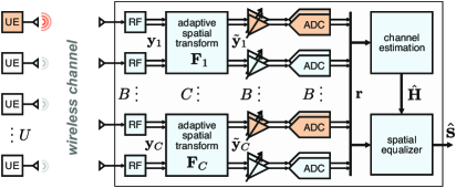
We now describe the HDR MIMO BS architecture depicted in \freffig:schematic, which is able to deal with receive signals of high dynamic range. In order to prevent weak UEs from drowning in quantization noise or strong UEs from saturating all ADCs, we introduce adaptive analog spatial transforms prior to the AGCs and ADCs. We focus on linear transforms represented by the matrices , , where each matrix operates on a cluster of antennas with such antenna clusters in total.111In practice, the number of antennas per cluster should not be too large as implementing large analog spatial transforms is challenging [19]. These adaptive analog spatial transforms implement
| (3) |
where is the th cluster of the receive vector and is the corresponding output of the adaptive analog spatial transform. The transformed receive vector is, therefore,
| (4) |
where and is a block diagonal matrix.
Note that if no structural constraints are imposed on the clusters of the adaptive analog spatial transform matrix , then \frefeq:y_tilde would have to be computed as a matrix-vector product consisting of complex-valued multiplications. However, the specific structure of the per-cluster transforms , , proposed in \frefsec:analogtransforms, enables simpler analog hardware with fewer complex-valued multiplications.
II-C Analog-to-Digital Conversion
As we will show in \frefsec:analogtransforms, the adaptive analog spatial transform ensures that only a subset of its outputs contains strong signals. One can then utilize the AGCs (cf. \freffig:schematic) to individually adjust the input gains for each pair of ADCs with the goal of minimizing saturation and quantization artifacts. In order to model such ADC artifacts, we follow [9, 10] and apply a uniform midrise quantizer to each entry of the real and imaginary parts of the transformed receive vector in \frefeq:y_tilde. The scalar function that models each ADC is given by
| (5) |
where is the quantizer’s step size and is the number of quantization bits. The distortions introduced by this model are then taken into account by the spatial equalizer (cf. \freffig:schematic).
To design the spatial equalizer, we employ Bussgang’s decomposition [20], where the effect of the quantizer on a real-valued zero-mean random variable (RV) is modeled as
| (6) |
with the so-called Bussgang gain
| (7) |
In \frefeq:bussgang_decomposition, the choice of as in \frefeq:buggang_gain ensures that the distortion is uncorrelated with and is zero mean with variance
| (8) |
In order to minimize the distortion caused by saturation and quantization, one can either pick an optimal step size while fixing the input variance or pick an optimal input variance while fixing the step size. We force the variance of the input to one and select an optimal step size that minimizes the mean squared error (MSE) between the quantizer’s output and its input [21]. To enforce unit variance at the inputs of all ADCs, we need to adjust the AGC settings, which we model by a diagonal gain control matrix with
| (9) |
Here, the covariance matrix is given by
| (10) |
By multiplying the gain control matrix to the transformed receive vector , the entries of have unit variance per real dimension. The resulting AGC and ADC model is
| (11) |
By applying Bussgang’s decomposition \frefeq:bussgang_decomposition individually to each entry of \frefeq:quantized_y_tilde, we obtain the following linearized input-output relation:
| (12) | ||||
| (13) | ||||
| (14) |
Here, we define , where and are the real and imaginary parts of the distortions caused by , respectively.
II-D Spatial Equalization
The linearized input-output relation in \frefeq:quantized_y_tilde_2 can now be used to design a linear minimum mean squared error (LMMSE)-type equalizer, which generates estimates for the transmitted symbols as . In the equalization step, we do not assume perfect knowledge of the channel matrix. Therefore, using the estimate of the channel matrix , we define our LMMSE-type equalization matrix as
| (15) |
where we approximate the distortion covariance matrix as
| (16) |
with from \frefeq:D_definition.
III Adaptive Analog Spatial Transforms
We are now ready to describe the specifics of suitable adaptive analog spatial transforms , , which we use to focus strong receive signals onto a subset of the ADCs. Specifically, we present two HR matrices designed for different purposes: HR-ISO, which isolates the energy of the strongest UE on dedicated ADCs, and HR-MAX, which isolates the signal dimension with the highest receive power on dedicated ADCs.
III-A Householder Reflections
An HR is carried out by multiplying a vector by a matrix that reflects the vector with respect to a subspace described by its normal vector [22, 23].
Definition 1.
Let be a nonzero vector. Then, the HR matrix is defined as follows:
| (17) |
HR matrices are (i) unitary so that the statistics of an i.i.d Gaussian random vector remain unaffected and (ii) Hermitian symmetric, i.e., .
By replacing in \frefeq:y_tilde_c with as in \frefeq:householder_matrix, we obtain a transformed receive vector in the th antenna cluster as
| (18) |
where . This operation requires only one inner-product calculation followed by subtracting a scaled version of from . Thus, the number of real- and complex-valued multiplications required to transform all antenna clusters decreases from to only , which can be implemented more efficiently, e.g., using analog multiplication circuitry originally developed for beamforming [24]. We reiterate that the statistics of the noise vector in \frefeq:received_vector remain unaffected by \frefeq:transformed_receive_vector_cluster since the matrices , , are unitary. Suitable choices for the vector are discussed next.
III-B Strongest UE Isolation (HR-ISO)
As the first choice for the HR matrix, we wish to isolate the energy of the strongest UE on the th output of the adaptive analog spatial transform. To this end, we need the following result; the proof is given in \frefapp:ISO.
Lemma 1.
Let be a nonzero vector. Then, the vector
| (19) |
is a solution of the following optimization problem:
| (20) |
We can use \freflem:HouseholderQR to isolate the energy of the strongest UE on the first pair of AGCs/ADCs of each antenna cluster by setting and , which corresponds to solving
| (21) |
where is the estimated channel vector associated with the th cluster of the strongest UE. According to \freflem:HouseholderQR, a vector that solves \frefeq:specificoptimizationproblem1 is
| (22) |
Therefore, the HR matrix that focuses the energy of the strongest UE on the first per-cluster AGCs and ADCs is . Note that is the standard HR vector used for QR decompositions applied to [23, Sec. 5.2.1].
III-C Maximum Power Isolation (HR-MAX)
As the second choice for the HR matrix, we wish to isolate the signal dimension with the highest receive power per antenna cluster on the th output of the adaptive analog spatial transform. To this end, we need the following result; the proof is given in \frefapp:MAX.
Lemma 2.
Let be a zero-mean random vector with covariance matrix . Furthermore, let be the eigenvector associated with the largest eigenvalue of the covariance matrix . Then, the vector
| (23) |
is a solution of the following optimization problem:
| (24) |
We can now use \freflem:maxpowerisolation to isolate the signal dimension with the highest receive power of antenna cluster on the first pair of AGCs/ADCs by setting and with , which corresponds to solving
| (25) |
According to \freflem:maxpowerisolation, a vector that solves \frefeq:specificoptimizationproblem2 is
| (26) |
where is the eigenvector associated with the largest eigenvalue of the covariance matrix . Therefore, the HR matrix that focuses the signal dimension with the highest receive power on the first per-cluster pair of AGCs and ADCs is .
IV Simulation Results
We now demonstrate the efficacy of HDR MIMO in a mmWave massive MU-MIMO scenario where one UE has significantly stronger BS-side receive power than the other UEs.


IV-A Simulation Details
We consider an uplink scenario in which single-antenna UEs transmit data to a BS with antennas arranged as a uniform linear array (ULA) with half-wavelength antenna spacing. The BS is at a height of m and the UEs at m; both the BS and the UEs are equipped with omnidirectional antennas. The system operates at a carrier frequency of GHz and a bandwidth of MHz. The UEs transmit 16-QAM symbols. We limit the BS-side receive power between the weakest and the second strongest UE by dB using the power control scheme in [25, Sec. II-B], which determines the per-UE gains , . In this scheme, strong UEs that exceed the dynamic range limit have to transmit with lower power while weak UEs transmit at their original power. We use mmWave channel vectors generated with Remcom’s Wireless InSite [1] for UE positions in an area of . For every channel realization, we select UE channel vectors uniformly at random. We define the median receive signal-to-noise ratio (MSNR) as follows:
| (27) |
The covariance matrix used in \frefeq:true_cy for the AGC matrix and in \frefeq:specificoptimizationproblem2 for solving HR-MAX is estimated as follows: . Here, the received matrix is obtained during pilot-based training (cf. \frefsec:system_model), where we use orthogonal pilot sequences of length taken from a properly scaled Hadamard matrix.
IV-B Baseline Algorithms
We compare the proposed HDR MIMO methods HR-ISO and HR-MAX to three baselines. The first baseline is called “Perfect” and considers the same simulation setup as for HDR MIMO, but uses a receiver with infinite-resolution ADCs. Therefore, it does not require any spatial transform. The second baseline is called “WSU” (short for “without strongest UE”) and considers a different simulation setup in which all UEs are power-controlled to a dynamic range of dB and no spatial transform is used. The third baseline is called “None” and assumes the same simulation setup as for the HDR MIMO methods but without any spatial transform. Thus, we have for all baselines.
IV-C Simulation Results
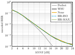
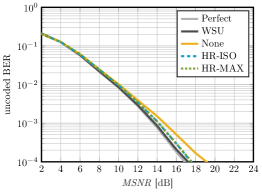
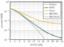
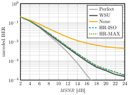
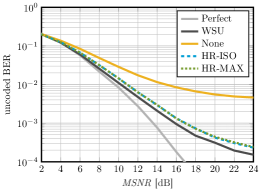
We evaluate the performance of HDR MIMO and the baseline algorithms in terms of uncoded bit error rate (BER).We vary three parameters from our system: the dynamic range from \frefeq:rho_definition, the number of ADC quantization bits from \frefeq:uniform_midrise_quantizer, and the number of antenna clusters from \frefeq:y_tilde_c. When varying one of these parameters, we fix all of the others to dB, bit, and antenna clusters.
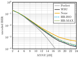
In \freffig:varying_rho, we show results varying the dynamic range . We observe that “Perfect,” which has infinite ADC resolution, outperforms all of the other presented methods which utilize 3-bit ADC resolution. As we increase the dynamic range , the MSNR gap between “WSU” and the proposed HDR MIMO methods (HR-ISO and HR-MAX) increases. However, even with a stronger BS-side receive power between the weakest and strongest UEs, our proposed methods maintain an MSNR gap of only dB at % BER between the HDR MIMO methods and “WSU”. Furthermore, the proposed HDR MIMO methods demonstrate significant performance gains compared to "None," especially for scenarios in which the BS-side receive power of the strongest UE far exceeds that of the other UEs (see \freffig:varying_rho_30). Hence, the benefits of HDR MIMO are more pronounced with increasing BS-side receive power of the strongest UE.
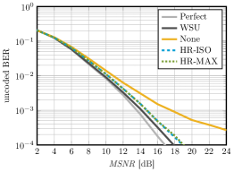
In \freffig:varying_q, we show results varying the number of quantization bits . In \freffig:varying_q_3, we observe a similar behavior as in \freffig:varying_rho, where “Perfect” outperforms all of the other presented methods due to its infinite ADC resolution. As we increase the number of quantization bits , the MSNR gap between “Perfect,” “WSU,” “None,” and the proposed HDR MIMO methods decreases, almost closing the MSNR gap in \freffig:varying_q_5. This observation indicates that the benefits of HDR MIMO are less pronounced if the ADC resolution increases. Although with -bit ADCs the HDR MIMO methods approach a nearly equivalent BER compared to the use of infinite-resolution ADCs, it also presents a smaller advantage when compared to “None.” Thus, HDR MIMO is suitable for systems with low-resolution ADCs.
In \freffig:varying_C, we show results varying the number of antenna clusters , and observe a similar behavior as the one from \freffig:varying_rho and \freffig:varying_q_3, where “Perfect” outperforms all of the other presented methods due to its infinite ADC resolution. As we increase the number of antenna clusters , the MSNR gap between “WSU” and the HDR MIMO methods also increases. However, even when we have four times as many antenna clusters as in \freffig:varying_C_8, we can still maintain a relatively small MSNR gap of only dB at % BER between the HDR MIMO methods and “WSU” (\freffig:varying_C_32). Furthermore, the HDR MIMO methods demonstrate significant performance gains compared to "None," especially in scenarios with fewer antenna clusters, as shown in \freffig:varying_C_8. Hence, the benefit of HDR MIMO improves with fewer antenna clusters (which is equivalent to more antennas per cluster), even though it is disadvantageous for hardware implementation [19].
Finally, we compare the BER performance between the two adaptive analog spatial transforms: HR-ISO and HR-MAX. In Figs. 2, 3, and 4, we find that the BER is nearly identical. In conclusion, both HDR MIMO methods are beneficial in systems featuring high dynamic range UEs and low-resolution ADCs. However, from a complexity perspective, HR-ISO is the preferable option as it does not require the calculation of the covariance matrix and an eigenvalue decomposition.
V Conclusions
We have proposed HDR MIMO, a novel approach that consists of an adaptive analog spatial transform which enables one to focus the energy of the strongest UE or the signal dimension with the highest receive power on a few ADCs in order to mitigate saturation and quantization artifacts caused by high dynamic range UEs in systems with low-resolution ADCs. Simulation results have shown that HDR MIMO greatly outperforms systems without spatial transforms. Furthermore, we have shown that (i) as the strongest UE BS-side receive power increases and (ii) as the quantization resolution decreases, the more pronounced the benefits of HDR MIMO become. Besides that, we have shown that, although transforming large antenna clusters is favorable, small analog spatial transforms that are more hardware friendly only slightly deteriorate the effectiveness of HDR MIMO.
Appendix A Proof of \freflem:HouseholderQR
The objective function of \frefeq:optimizationproblem1 is bounded by
| (28) |
Here, follows from the Cauchy–Schwarz inequality and from the fact that is unitary. We now show that the HR matrix with the vector from \frefeq:solutionoptimizationproblem1 achieves the upper bound in \frefeq:cauchy_schwarz with equality. To this end, notice that the Cauchy–Schwarz inequality holds with equality if and only if and are collinear, i.e., if holds for some . From \frefeq:householder_matrix, it follows that
| (29) |
From \frefeq:new1, after some algebraic manipulations, we arrive at
| (30) |
where we assume that , i.e., and are not orthogonal. By inserting from \frefeq:new2 into \frefeq:new1, the following must hold:
| (31) |
Since the factor from \frefeq:new2 cancels out, its specific choice does not matter (assuming that it is nonzero). Therefore, we assume in what follows.
In order to determine the optimal value of , we first assume that . By rearranging terms in \frefeq:new3, we obtain the following necessary optimality condition
| (32) |
which can be simplified to
| (33) |
This equation has two solutions . By inserting into \frefeq:new3, both the left and right sides are equal, proving that the two solutions are indeed solutions to \frefeq:new3. For reasons given below, we pick the solution
| (34) |
Let us now inspect the two excluded cases and . If , then the vectors and are orthogonal. With \frefeq:solutionoptimizationproblem1, this implies that
| (35) |
which is impossible as the vector was assumed to be nonzero; this is the reason why we picked the solution in \frefeq:alphaopt. If , then according to \frefeq:solutionoptimizationproblem1, . By plugging this vector into \frefeq:optimizationproblem1, the bound in \frefeq:cauchy_schwarz is achieved with equality.
In summary, by combining \frefeq:new2 and \frefeq:alphaopt, we see that a vector that maximizes \frefeq:optimizationproblem1 is given by \frefeq:solutionoptimizationproblem1.
Appendix B Proof of \freflem:maxpowerisolation
With the covariance matrix , we can rewrite the optimization problem in \frefeq:optimizationproblem2 as
| (36) |
We can now bound the objective of \frefeq:optimizationproblem4 as follows:
| (37) |
Here, holds as is a specific unit-norm vector and taking the maximum over arbitrary unit-norm vectors bounds the objective. The equality follows from the definition of the spectral norm, which is equal to the largest eigenvalue of the covariance matrix of [26, Ex. 5.6.6]. We now show that the HR matrix with from \frefeq:solutiontooptimizationproblem2 achieves the upper bound in \frefeq:upperbound with equality.
We start by rewriting \frefeq:optimizationproblem4 as follows:
| (38) |
Here, the expression with from \frefeq:solutiontooptimizationproblem2 is bounded by
| (39) |
where follows from the Cauchy–Schwarz inequality and from the fact that is unitary. From \freflem:HouseholderQR, we know that using from \frefeq:solutiontooptimizationproblem2 leads to equality in , i.e., . This conclusion together with the objective from \frefeq:newoptimizationproblem4 leads to
| (40) |
since the eigenvalues , are nonnegative. By combining \frefeq:upperbound and \frefeq:lowerbound, we conclude that the objective function in \frefeq:newoptimizationproblem4 is both lower and upper bounded by . Thus, with from \frefeq:solutiontooptimizationproblem2, we have that
| (41) |
which completes the proof.
References
- [1] Remcom, Inc. (2023) Wireless InSite. [Online]. Available: https://www.remcom.com/wireless-insite-em-propagation-software
- [2] A. L. Swindlehurst, E. Ayanoglu, P. Heydari, and F. Capolino, “Millimeter-wave massive MIMO: the next wireless revolution?” IEEE Commun. Mag., vol. 52, no. 9, pp. 56–62, Sep. 2014.
- [3] S. Dutta, C. N. Barati, D. Ramirez, A. Dhananjay, J. F. Buckwalter, and S. Rangan, “A case for digital beamforming at mmWave,” IEEE Trans. Wireless Commun., vol. 19, no. 2, pp. 756–770, Feb. 2020.
- [4] S. H. Mirfarshbafan, A. Gallyas-Sanhueza, R. Ghods, and C. Studer, “Beamspace channel estimation for massive MIMO mmWave systems: Algorithm and VLSI design,” IEEE Trans. Circuits Syst. I, vol. 67, no. 12, pp. 5482–5495, Sep. 2020.
- [5] S. Jacobsson, G. Durisi, M. Coldrey, U. Gustavsson, and C. Studer, “Throughput analysis of massive MIMO uplink with low-resolution ADCs,” IEEE Trans. Wireless Commun., vol. 16, no. 6, pp. 4038–4051, Jun. 2017.
- [6] B. C. Geiger, C. Feldbauer, and G. Kubin, “Information loss in static nonlinearities,” in IEEE Int. Symp. Wireless Commun. Syst., Nov. 2011, pp. 799–803.
- [7] H. Subbaram and K. Abend, “Interference suppression via orthogonal projections: a performance analysis,” IEEE Trans. Antennas Propag., vol. 41, no. 9, pp. 1187–1194, Sep. 1993.
- [8] Q. Yan, H. Zeng, T. Jiang, M. Li, W. Lou, and Y. T. Hou, “MIMO-based jamming resilient communication in wireless networks,” in IEEE Conf. Comput. Commun. (INFOCOM), May 2014, pp. 2697–2706.
- [9] G. Marti, O. Castañeda, S. Jacobsson, G. Durisi, T. Goldstein, and C. Studer, “Hybrid jammer mitigation for all-digital mmWave massive MU-MIMO,” in Asilomar Conf. Signals, Syst., Comput., Nov. 2021, pp. 93–99.
- [10] G. Marti, O. Castañeda, and C. Studer, “Jammer mitigation via beam-slicing for low-resolution mmWave massive MU-MIMO,” IEEE Open J. Circuits Syst., vol. 2, pp. 820–832, Dec. 2021.
- [11] M. A. Alaei, S. Golabighezelahmad, P.-T. de Boer, F. E. van Vliet, E. A. M. Klumperink, and A. B. J. Kokkeler, “Interference mitigation by adaptive analog spatial filtering for MIMO receivers,” IEEE Trans. Microw. Theory Tech., vol. 69, no. 9, pp. 4169–4179, May 2021.
- [12] A. Bhandari, F. Krahmer, and R. Raskar, “On unlimited sampling and reconstruction,” IEEE Trans. Signal Process., vol. 69, pp. 3827–3839, 2021.
- [13] A. Bhandari, F. Krahmer, and T. Poskitt, “Unlimited sampling from theory to practice: Fourier-prony recovery and prototype ADC,” IEEE Trans. Signal Process., vol. 70, pp. 1131–1141, 2022.
- [14] Z. Liu, A. Bhandari, and B. Clerckx, “–MIMO: Massive MIMO via modulo sampling,” IEEE Trans. Commun., pp. 1–1, 2023.
- [15] D. Tse and P. Viswanath, Fundamentals of Wireless Communication. Cambridge Univ. Press, 2005.
- [16] M. Chiang, P. Hande, T. Lan, and C. W. Tan, Power Control in Wireless Cellular Networks. Now Foundations and Trends, 2008.
- [17] V. Saxena, G. Fodor, and E. Karipidis, “Mitigating pilot contamination by pilot reuse and power control schemes for massive MIMO systems,” in IEEE Veh. Technol. Conf. Spring (VTC-Spring), May 2015, pp. 1–6.
- [18] E. Björnson, J. Hoydis, and L. Sanguinetti, Massive MIMO Networks: Spectral, Energy, and Hardware Efficiency. Now Foundations and Trends, 2017.
- [19] Z. M. Enciso, S. Hadi Mirfarshbafan, O. Castañeda, C. J. Schaefer, C. Studer, and S. Joshi, “Analog vs. digital spatial transforms: A throughput, power, and area comparison,” in IEEE Int. Midwest Symp. Circuits Syst. (MWSCAS), Aug. 2020, pp. 125–128.
- [20] J. J. Bussgang, “Crosscorrelation functions of amplitude-distorted Gaussian signals,” Res. Lab. Elec., Cambridge, MA, USA, Tech. Rep. 216, Mar. 1952.
- [21] J. Max, “Quantizing for minimum distortion,” IRE Trans. Inf. Theory, vol. 6, no. 1, pp. 7–12, Mar. 1960.
- [22] L. N. Trefethen and D. Bau, Numerical Linear Algebra. SIAM, 1997.
- [23] G. H. Golub and C. F. Van Loan, Matrix Computations, 3rd ed. The Johns Hopkins University Press, 1996.
- [24] E. Naviasky, L. Iotti, G. LaCaille, B. Nikolić, E. Alon, and A. M. Niknejad, “A 71-to-86-GHz 16-element by 16-beam multi-user beamforming integrated receiver sub-array for massive MIMO,” IEEE J. Solid-State Circuits, vol. 56, no. 12, pp. 3811–3826, Dec. 2021.
- [25] H. Song, T. Goldstein, X. You, C. Zhang, O. Tirkkonen, and C. Studer, “Joint channel estimation and data detection in cell-free massive MU-MIMO systems,” IEEE Trans. Wireless Commun., vol. 21, no. 6, pp. 4068–4084, Jun. 2022.
- [26] R. A. Horn and C. R. Johnson, Matrix Analysis, 2nd ed. Cambridge University Press, 2013.