Generating Collective Counterfactual Explanations in Score-Based Classification via Mathematical Optimization

Abstract

Due to the increasing use of Machine Learning models in high stakes decision making settings, it has become increasingly important to have tools to understand how models arrive at decisions. Assuming an already trained Supervised Classification model, post-hoc explanations can be obtained via so-called counterfactual analysis: a counterfactual explanation of an instance indicates how this instance should be minimally modified so that the perturbed instance is classified in the desired class by the given Machine Learning classification model.

Most of the Counterfactual Analysis literature focuses on the single-instance single-counterfactual setting, in which the analysis is done for one single instance to provide one single counterfactual explanation. Taking a stakeholder’s perspective, in this paper we introduce the so-called collective counterfactual explanations. By means of novel Mathematical Optimization models, we provide a counterfactual explanation for each instance in a group of interest, so that the total cost of the perturbations is minimized under some linking constraints. Making the process of constructing counterfactuals collective instead of individual enables us to detect the features that are critical to the entire dataset to have the individuals classified in the desired class. Our methodology allows for some instances to be treated individually, as in the single-instance single-counterfactual case, performing the collective counterfactual analysis for a fraction of records of the group of interest. This way, outliers are identified and handled appropriately.

Under some assumptions on the classifier and the space in which counterfactuals are sought, finding collective counterfactual explanations is reduced to solving a convex quadratic linearly constrained mixed integer optimization problem, which, for datasets of moderate size, can be solved to optimality using existing solvers.

The performance of our approach is illustrated on real-world datasets, demonstrating its usefulness.

Keywords— Collective Counterfactual Explanations; Mathematical Optimization; Explainable Machine Learning; Linear Models; Random Forests

1 Introduction

There is an unprecedented need for transparency and interpretability in Machine Learning, i.e., explaining how models arrive at decisions (Ahani et al., 2021; Jung et al., 2020; Miller, 2019; Zhang et al., 2019). This includes selecting the features that impact the most the model as a whole (Benítez-Peña et al., 2021; Bertsimas et al., 2016; Hazimeh and Mazumder, 2020; Zheng et al., 2021), but also locally to the decision made for a given individual (Lundberg and Lee, 2017; Ribeiro et al., 2016). Given an already trained Supervised Classification model, an effective class of post-hoc explanations consists of the so-called counterfactual explanations (Martens and Provost, 2014; Wachter et al., 2017), identifying the actions to be taken by an instance (e.g., increase a given amount the salary, decrease the current debt of an individual by a given percentage) such that the Machine Learning model at hand would have classified it in the desired class (e.g., the loan request is granted to the individual).

Methods to build counterfactual explanations for Supervised Classification can be widely divided into model-agnostic or model-specific. The former treat the classification model as a black-box and do not use its inner workings (Dandl et al., 2020; Guidotti et al., 2019; Poyiadzi et al., 2020), whereas the latter do. One of the first model-specific approaches was proposed by Wachter et al. (2017), where the problem of finding a counterfactual explanation for an instance is formulated as an optimization model, but the numerical solution approach is limited to differentiable classification models (Joshi et al., 2019; Ramakrishnan et al., 2020). Other model-specific approaches have been proposed for linear classification models (Navas-Palencia, 2021; Ustun et al., 2019), tree-based models (Cui et al., 2015; Fernández et al., 2020; Parmentier and Vidal, 2021) or neural networks (Dhurandhar et al., 2018; Le et al., 2020). When differentiability holds, gradient-based algorithms are often proposed to solve the so-obtained optimization problems (Joshi et al., 2019; Le et al., 2020; Wachter et al., 2017). Otherwise, it is common to find mixed integer programming algorithms (Carrizosa et al., ; Fischetti and Jo, 2018; Kanamori et al., 2020, 2021; Maragno et al., 2022; Russell, 2019). See Karimi et al. (2022); Verma et al. (2022) for recent surveys and also Browne and Swift (2020); Freiesleben (2022) for works on adversarial learning, with well-known applications in, e.g., image analysis.

The approaches mentioned above, either model-agnostic or model-specific, are all single-instance single-counterfactual (one counterfactual is sought for just one instance) models. In this paper we depart from such approaches, and, taking a stakeholder perspective, we focus on the generation of collective counterfactual explanations, where a counterfactual is obtained for each instance of a specific group of interest, which may represent the people of certain age, gender, race, or just the whole set of individuals who were not classified in the desired class by the Machine Learning classifier. There are different reasons to compute the counterfactual explanations for a group of instances instead of computing them separately. First, stakeholders may want to identify a small set of features that need to be modified to alter the prediction of the instances in a group of interest. In the literature, it is often argued that sparser counterfactuals are desired, as having fewer features changed may be more interpretable for an individual, see Carrizosa et al. (2023); Miller (2019); Verma et al. (2022) and references therein. As we are dealing with a group of instances, on top of counting the number of features perturbed for each instance, with our methodology we can also take into account the total number of features perturbed, allowing us to identify which features are critical to alter the class prediction given to a group of interest by the classifier.

Second, there may be some instances that do not behave like the rest of the group, and by perturbing them we would incur very high costs. These instances may be outliers to the group, and it is important to identify them to be treated separately. Whereas outliers’ identification is a well studied topic in data analysis, e.g. Boukerche et al. (2020), as far as the authors are aware, this issue has not been addressed so far in the literature on counterfactual explanations.

Assuming that a dissimilarity or a distance in the space of instances is given, we propose a mathematical optimization model that minimizes a cost measure of the dissimilarity between the given instances and the collective counterfactual instances. Desirable properties are accommodated by the model as well. In particular, one can control the number of features to be perturbed in order to have all individuals in the group of interest classified in the desired class. This means, in the loan application example, to identify the minimum number of changes needed for the group of interest to be granted the loan request, that prior to perturbing the features were rejected. Constraints on the counterfactuals are easily accommodated as well (Maragno et al., 2022; Mohammadi et al., 2021; Wachter et al., 2017). Our model also allows a certain fraction of records to be treated separately and individually, as in the single-instance single-counterfactual case, and the collective counterfactual analysis is thus performed for just a fraction of records of the group of interest. This way, outliers in the group of interest are properly identified and handled appropriately.

Although our approach is applicable to any classification model based on scores, Carrizosa and Romero Morales (2013), we focus in what follows on models with some linear structure, such as logistic regression or additive trees like Random Forests or XGBoost. Under mild assumptions on the set defining the feasible perturbations, our optimization model is expressed as a Mixed Integer Convex Quadratic Model with linear constraints, which can be solved with standard optimization packages.

The remainder of the paper is organized as follows. In Section 2, we formalize the model and introduce the optimization problem that obtains collective counterfactual explanations for score-based classifiers. We detail this formulation for a specific cost function, accounting for the perturbations as well as the number of features changed, and for two families of classifiers, namely, a logistic regression model and additive tree models. In Section 3, numerical illustrations for real-world datasets can be found. We end the paper with Section 4, where conclusions and possible lines of future research are provided. The appendix contains a detailed discussion of the formulation for the model for additive trees. The supplementary material contains some of the illustrations from the numerical section.

2 Problem Statement

2.1 Collective counterfactuals

In this section we formalize the problem of finding collective counterfactual explanations. We first discuss the main ingredients of the model, namely, the admissible perturbations, the way perturbations costs are measured, and the baseline classifier. We then address an easy but relevant case, namely, the separable case, which reduces the problem to solving a series of single-instance single-counterfactual problems. Then, for the non-separable case, a mixed integer programming formulation is given.

Let us consider a binary classification problem, with classes denoted by $+1,-1$, in a set $\mathcal{X}\subset\mathbb{R}^{J}$. The class $+1$ represents something positive for the individual, such as receiving social benefits or having a loan request granted, while the negative class $-1$ refers to something negative, such as not having access to those benefits or having the loan request denied. Having the data in $\mathbb{R}^{J}$ does not mean that all features considered are numerical ones. Indeed, if we have categorical features, we can transform them into numerical ones using the standard one-hot encoding.

We assume given a so-called score-based classifier, i.e., one has a function $f:\mathcal{X}\longrightarrow\mathbb{R}$, so that instance $\bm{x}$ is assigned to the positive class if $f(\bm{x})\geq\nu$, for a given threshold value $\nu$. For an instance $\bm{x}^{0},$ its counterfactual is an instance $\bm{x}$ in the feasible set $\mathcal{X}^{0}\subset\mathcal{X}$, classified in the positive class, i.e., $f(\bm{x})\geq\nu,$ such that the cost of perturbing $\bm{x}^{0}$ to $\bm{x}$ is minimal.

Instead of finding the counterfactual for a specific instance $\bm{x}^{0}$, in this paper we address the problem of building simultaneously collective counterfactual explanations, i.e., explanations for a group of instances.

Let us formalize these ideas and express the search of collective counterfactuals as a mathematical optimization problem. Let $\bm{\underline{x}}^{0}=(\bm{x}^{0}_{1},\dots,\bm{x}^{0}_{I})$ be $I$ instances, which form the group of interest, and let $\mathcal{I}^{*}\subset\{1,\dots,I\}$ be the sought subset of cardinality $I^{*}$ corresponding to the indices of the instances to be perturbed so that the classifier would classify them all in the positive class. Let $\mathcal{\underline{X}}^{0}$ be the feasible region of the set of counterfactuals $\bm{\underline{x}}:=(\bm{x}_{1},\dots,\bm{x}_{I})$, where $\mathcal{\underline{X}}^{0}\subset\prod_{i}\mathcal{X}^{0}_{i}$ with $\mathcal{X}^{0}_{i}$ being the feasible set for the counterfactual of instance $i$, assumed to be a compact set.

The set $\mathcal{\underline{X}}^{0}$ includes different constraints that should be satisfied by each single counterfactual (Maragno et al., 2022; Mohammadi et al., 2021; Wachter et al., 2017). The set can be a finite collection of datapoints, yielding the so-called endogenous counterfactuals (Smyth and Keane, 2022; Wiratunga et al., 2021), or defined as a convex combination of known datapoints (Brughmans et al., 2023). Alternatively, the counterfactual can be synthetically built, yielding in this case the so-called exogenous explanations. The latter is the most popular approach in the literature (Guidotti, 2022). Further constraints may have to be satisfied, for instance, some features such as gender or race cannot be perturbed, for some features such as salary we need to ensure their non-negativity, while for categorical features such as employment status exactly one category should be chosen for each counterfactual instance. In addition to these individual constraints, constraints that may link the counterfactual instances $\bm{\underline{x}}$ can also appear naturally. For instance, for a categorical feature, we may want that the counterfactuals for all the instances in the group of interest are evenly distributed across all the categories. Doing so, one could avoid unrealistic scenarios, such as requiring all individuals to be in the highest income bracket.

Let $C(\bm{\underline{x}}^{0},\bm{\underline{x}})$ be the function that measures the cost of perturbing $\bm{\underline{x}}^{0}$ to $\bm{\underline{x}}\in\mathcal{\underline{X}}^{0}.$ Although our approach is valid for more general settings, we will consider in what follows a parametrized family of cost functions $C:$

$$C(\bm{\underline{x}}^{0},\bm{\underline{x}})=\sum_{i=1}^{I}\|\bm{x}^{0}_{i}-\bm{x}_{i}\|_{2}^{2}+\lambda_{ind}\sum_{i=1}^{I}\|\bm{x}_{i}^{0}-\bm{x}_{i}\|_{0}+\lambda_{glob}\gamma_{0}(\underline{\bm{x}}^{0},\underline{\bm{x}}).$$ (1)

The first term in (1) is an overall measure of the perturbations (measured through the Euclidean distance) to move from $\bm{\underline{x}}^{0}$ to $\bm{\underline{x}}.$ The second term measures, weighted by $\lambda_{ind}\geq 0$, the overall number of perturbations in features needed to move from $\bm{\underline{x}}^{0}$ to $\bm{\underline{x}}.$ Finally, $\gamma_{0}$ is given by

$$\gamma_{0}(\underline{\bm{x}}^{0},\underline{\bm{x}})=\left\|\left(\max_{1\leq i\leq I}|x_{ij}^{0}-x_{ij}|\right)_{j=1}^{J}\right\|_{0},$$ (2)

where $x_{ij}$ denotes the value of feature $j$ of instance $\bm{x}_{i}$. Notice that $\left(\max_{1\leq i\leq I}|x_{ij}^{0}-x_{ij}|\right)_{j=1}^{J}$ is a vector of $J$ components, where each component is the maximum change across all the instances. Hence, the third term measures, weighted by $\lambda_{glob}\geq 0,$ the number of features perturbed ever to move from $\bm{\underline{x}}^{0}$ to $\bm{\underline{x}}.$

2.2 Problem formulation

Given the score-based classifier induced by the score function $f,$ the feasible set $\mathcal{\underline{X}}^{0}$ and the cost function $C$ as in (1), the mathematical optimization formulation of finding the minimal cost perturbations of the features to classify $I^{*}$ instances in the positive class reads as follows:

$$\small\min_{\bm{\underline{x}},\mathcal{I}^{*}}\quad C(\bm{\underline{x}},\bm{\underline{x}}^{0})$$ (ColCE)

s.t. $$f(\bm{x}_{i})\geq\nu\quad\forall i\in\mathcal{I}^{*}$$ (3)

$$\bm{x}_{i}=\bm{x}_{i}^{0}\quad\forall i\notin\mathcal{I}^{*}$$ (4)

$$|\mathcal{I}^{*}|=I^{*}$$ (5)

$$\bm{\underline{x}}\in\mathcal{\underline{X}}^{0}.$$ (6)

Let us first address an easy yet very relevant case. When $\lambda_{glob}=0,$ i.e., when the perturbation cost is measured by the sum of the squared Euclidean distances and the $\ell_{0}$ norm between each $\bm{x}^{0}_{i}$ and its corresponding individual counterfactual $\bm{x}_{i},$ then $C$ is separable. Moreover, when there are no linking constraints in $\mathcal{\underline{X}}^{0}$, i.e., when $\mathcal{\underline{X}}^{0}=\prod_{i=1}^{I}\mathcal{X}^{0}_{i}$, then Problem (ColCE) is separable as well. This way, the problem can be split into $I$ individual counterfactual problems, linked just by the constraint (5). This yields the following:

Proposition 2.1.

Suppose $\lambda_{glob}=0,$ and $\mathcal{\underline{X}}^{0}=\prod_{i=1}^{I}\mathcal{X}^{0}_{i}$. For $i=1,\dots,I,$ let $\bm{x}^{*}_{i}$ be an optimal solution of the single-instance single-counterfactual problem

$$\small\min_{\bm{x}_{i}}\quad \|\bm{x}^{0}_{i}-\bm{x}_{i}\|_{2}^{2}+\lambda_{ind}\|\bm{x}_{i}^{0}-\bm{x}_{i}\|_{0}$$ (CEsep)

s.t. $$f(\bm{x}_{i})\geq\nu$$ (7)

$$\bm{x}_{i}\in\mathcal{X}^{0}_{i}.$$

Then an optimal solution for Problem (ColCE) is obtained by sorting the costs $\|\bm{x}_{i}^{0}-\bm{x}_{i}^{*}\|_{2}^{2}+\lambda_{ind}\|\bm{x}_{i}^{0}-\bm{x}_{i}^{*}\|_{0}$ and selecting the $I^{*}$ instances with the lowest value of such cost.

In what follows, we address the case in which the separability assumptions above do not hold. Let us express then (ColCE) in a more tractable form, by first rewriting the objective function as a quadratic convex function, and then rewriting the constraints (3)-(5), so that, when $\mathcal{\underline{X}}^{0}$ is polyhedral (eventually with some coordinates in integer numbers), a mixed integer convex quadratic program is obtained.

In order to linearize the $\ell_{0}$ norm and $\gamma_{0}$ in (2), binary variables are introduced. For every feature $j$ and every instance $i$, define the binary variable $\xi_{ij}$ with $\xi_{ij}=1$ if feature $j$ of instance $i$ is perturbed, i.e., $x_{ij}\neq x_{ij}^{0}$. The $\ell_{0}$ norm is linearized by adding to the model following constraints:

$$-M_{ij}\xi_{ij}\leq x^{0}_{ij} -x_{ij}\leq M_{ij}\xi_{ij}\quad j=1,\dots,J,i=1,\dots,I$$ (8)

$$\xi_{ij} \in\{0,1\},$$ (9)

where each $M_{ij}$ is a big constant, which exists thanks to the bounded nature of $\mathcal{\underline{X}}^{0}.$ In particular, any

$$M_{ij}\geq|x_{ij}^{0}|+\max_{\bm{z}\in\mathcal{X}^{0}_{i}}|z_{j}|$$ (10)

is valid.

A similar linearization can be done for the global sparsity $\gamma_{0}$. In that case, a binary variable $\xi^{*}_{j}$ is introduced. For each feature $j$, $\xi_{j}^{*}$ takes the value 1 if $x_{ij}$ takes a value different from $x_{ij}^{0}$ for some instance $i=1,\dots,I$. The following constraints are added to our formulation:

$$\xi_{j}^{*}\geq \xi_{ij}\quad i=1,\dots,I,j=1,\dots J$$ (11)

$$\xi_{j}^{*} \in\{0,1\}\quad j=1,\dots,J.$$ (12)

Moreover, in order to indicate whether an instance is perturbed or not, new binary variables $\bm{y}$ are introduced. For $i=1,\dots,I$, $y_{i}=1$ if instance $i$ is allowed to be perturbed, and $y_{i}=0$ otherwise. Then constraints (3) and (5) are expressed respectively as

$$y_{i}(f(\bm{x}_{i})-\nu)\geq 0\quad i=1,\dots,I.$$ (13)

and

$$\sum_{i=1}^{I}y_{i}=I^{*}$$ (14)

Notice that when using cost function (1), as we are minimizing the Euclidean norm, if $y_{i}=0$, then $\bm{x}_{i}=\bm{x}_{i}^{0}$ automatically, so constraint (4) can be omitted.

We end this section by rewriting constraint (13) in a more tractable form for the case of a linear classifier, such as the one in the logistic regression. The formulation for additive tree models (ATM), e.g., Random Forest or XGBoost models, can be found in the Appendix. Additionally, the methodology can be applied to neural networks, specifically to Feed Forward Neural Networks with ReLU activation and other well-known score-based models, see Carrizosa et al. (2023).

In the logistic regression model, the score function is given by $\bm{w}\bm{x}+b,$ and thus constraint (13) takes the form:

$$(\bm{w}\bm{x}_{i}+b)y_{i}\geq\nu y_{i}\quad i=1,\dots,I.$$

We can linearize this new constraint using the usual Fortet linearization technique (Fortet, 1960). We introduce a new decision variable $u_{i}$ to model the product $(\bm{w}\bm{x}_{i}+b)y_{i}$. The following constraints need to be added to our model:

$$u_{i}\geq\nu y_{i}\qquad i=1,\dots,I$$ (15)

$$u_{i}\leq y_{i}M_{i}^{*}\qquad i=1,\dots,I$$ (16)

$$u_{i}\geq-y_{i}M_{i}^{*}\qquad i=1,\dots,I$$ (17)

$$u_{i}\leq(\bm{w}\bm{x}_{i}+b)+(1-y_{i})M_{i}^{*}\qquad i=1,\dots,I$$ (18)

$$u_{i}\geq(\bm{w}\bm{x}_{i}+b)-(1-y_{i})M_{i}^{*}\qquad i=1,\dots,I$$ (19)

$$u_{i}\in\mathbb{R}\qquad i=1,\dots,I$$ (20)

$$y_{i}\in\{0,1\}\qquad i=1,\dots,I,$$ (21)

where each $M_{i}^{*}$ is a big constant. Using the bounded nature of $\mathcal{\underline{X}}^{0}$ as before, any

$$M_{i}^{*}\geq|b|+\|\bm{w}\|_{2}\max_{\bm{z}\in\mathcal{X}_{i}^{0}}\|\bm{z}\|_{2}$$ (22)

is valid.

Hence, the formulation of Problem (ColCE) for a logistic regression model with cost function (1) is as follows:

$$\begin{split}\min_{\underline{\bm{x}},\bm{y},\bm{\xi},\bm{\xi^{*}},\bm{u}}\quad&\sum_{i=1}^{I}\|\bm{x}_{i}^{0}-\bm{x}\|_{2}^{2}+\lambda_{ind}\sum_{i=1}^{I}\sum_{j=1}^{J}\xi_{ij}+\lambda_{glob}\sum_{j=1}^{J}\xi^{*}_{j}\\ \text{s.t.}\quad&\eqref{eq:cons_plaus},\eqref{eq:l0i},\eqref{eq:l0i2}\\ &\eqref{eq:l0g1},\eqref{eq:l0g2},\eqref{eq:cons_i22}-\eqref{eq:fortet5}.\end{split}$$ (ColCELR)

Assuming $\mathcal{\underline{X}}^{0}$ to be a bounded polyhedron with some integer coordinates, Problem (ColCELR) is a Mixed Integer Convex Quadratic Model with linear constraints. Therefore, it can be solved using a Mixed Integer Linear Programming (MILP) solver.

3 Numerical illustration

We will illustrate our methodology using real-world data. We have carried out the experiments in 4 datasets. Table 1 reports their name, source of origin, number of instances, number of total features and their type. All these datasets include heterogeneous feature types.

Name	Source	Number of instances	Number of features	Continuos	Ordinal	Binary	Nominal
Boston	Sklearn	506	14	13	0	1	0
COMPAS	ProPublica	6172	5	0	2	2	1
Credit	UCI	29623	14	4	7	3	0
Students	UCI	395	30	1	12	13	4

Table 1: Datasets used for the numerical experiments

In this section, we detail the results for the Boston housing dataset (Harrison Jr and Rubinfeld, 1978), which is derived from information collected by the U.S. Census Service concerning housing in the area of Boston. We have accessed it from the scikit-learn library (Pedregosa et al., 2011). There are 506 instances and 13 features. The description of the dataset can be found in Table 2. We have a binary classification problem, where where class $+1$ corresponds to the price of an instance being higher than the median value, and $-1$ otherwise.

Variable	Definition	Type
CRIM	per capita crime rate by town	numerical
ZN	proportion of residential land zoned for lots over 25,000 sq.ft	numerical
INDUS	proportion of non-retail business acres per town	numerical
CHAS	Charles River dummy variable (1 if tract bounds river; 0 otherwise)	binary
NOX	nitric oxides concentration (parts per 10 million)	numerical
RM	average number of rooms per dwelling	numerical
AGE	proportion of owner-occupied units built prior to 1940	numerical
DIS	weighted distances to five Boston employment centres	numerical
RAD	index of accessibility to radial highways	numerical
TAX	full-value property-tax rate per $10,000	numerical
PTRATIO	pupil-teacher ratio by town	numerical
B	$1000(Bk-0.63)^{2}$ where Bk is the proportion of blacks by town	numerical
LSTAT	% lower status of the population	numerical
MEDV	$+1$ if Median value of owner-occupied homes in $1000’s over the 50th percentile, $-1$ otherwise	target

Table 2: Description of the features of the Boston housing dataset

The results for the rest of the datasets are detailed in the supplementary material.

Two classifiers are constructed, namely, a logistic regression model and a Random Forest with $T=100$ trees and maximum depth of 4. In all the optimization problems solved, in $\mathcal{\underline{X}}^{0}$ we only impose the binary nature of variable CHAS and lower and upper bounds of each feature to be the minimum and maximum value observed across the 506 observations, respectively.

Solving collective counterfactual explanations for these two classifiers boils down to solving problems (ColCELR) and (ColCEATM). In addition, we illustrate the separable case (CEsep), in which constraint (7) has been rewritten in a more tractable way for the logistic regression model as we have done in (ColCELR), and for the Random Forest as in (ColCEATM). These formulations have been implemented using Pyomo optimization modeling language (Hart et al., 2017, 2011) in Python 3.7. As solver, we have used Gurobi 9.0 (Gurobi Optimization, 2021). A value of $\epsilon=1\mathrm{e}{-5}$ has been imposed in formulation (ColCEATM) and (CEsep) for the Random Forest. The values of the big-$M$ constants used are defined in (10), (22), (27) and (28). Our experiments have been conducted on a PC, with an Intel R CoreTM i7-1065G7 CPU @ 1.30GHz 1.50 GHz processor and 16 gigabytes RAM. The operating system is 64 bits. All experiments have been solved to optimality. The source code and the data to reproduce all results are available at https://github.com/jasoneramirez/CollectiveCE.

To visualize the counterfactual explanations, different heatmaps are displayed. In each of them, it is indicated the minimum cost perturbations needed for each instance to change its predicted class. Each column represents a feature and each row an instance. We present the difference between the original value of the feature and the new one from the counterfactual. A positive value for a feature means that the feature value would have to be higher in order to change the class of the instance, and a negative one indicates that the feature value should be lower.

First, counterfactual explanations for 10 individuals that were classified originally in the negative class by both classifiers, are calculated. The original values of the 10 instances can be seen in Table 3. The counterfactuals are calculated with cost function (1) with two different combinations of the values of $\lambda_{ind}$ and $\lambda_{glob}$. Specifically, in the first case, see Figure 1, we consider $\lambda_{ind}=0.02$ and $\lambda_{glob}=0$. In such case, as there are no other linking constraints in $\mathcal{\underline{X}}^{0}$, the problem is separable, so it is equivalent to solving 10 optimization problems of the form (CEsep), see Proposition 2.1. In the second case, see Figure 2, we consider $\lambda_{ind}=0$ and $\lambda_{glob}=0.2$. Now, global sparsity is sought. In all four situations, $I^{*}=I=10$ and we choose $\nu$ such that all the counterfactuals are classfied in the positive class, thus for the logistic regression model $\nu=0$ and for the Random Forest $\nu=0.5$.

CRIM	ZN	INDUS	CHAS	NOX	RM	AGE	DIS	RAD	TAX	PTRATIO	B	LSTAT
0.001840	0.125	0.271628	0.0	0.286008	0.468097	0.854789	0.496731	0.173913	0.236641	0.276596	0.974305	0.424117
0.002399	0.000	0.236437	0.0	0.129630	0.391071	0.608651	0.450863	0.086957	0.087786	0.563830	1.000000	0.399283
0.001607	0.250	0.171188	0.0	0.139918	0.417705	0.651905	0.554320	0.304348	0.185115	0.755319	0.995486	0.315121
0.015820	0.000	0.700880	1.0	1.000000	0.492048	0.958805	0.056361	0.173913	0.412214	0.223404	0.808664	0.369481
0.002870	0.000	0.346041	0.0	0.327160	0.471738	0.901133	0.154989	0.130435	0.223282	0.617021	0.998487	0.275662
0.124781	0.000	0.646628	0.0	0.582305	0.257712	1.000000	0.004056	1.000000	0.914122	0.808511	1.000000	0.911700
0.274109	0.000	0.646628	0.0	0.648148	0.209044	1.000000	0.030700	1.000000	0.914122	0.808511	1.000000	0.732616
0.430994	0.000	0.646628	0.0	0.633745	0.362522	1.000000	0.032736	1.000000	0.914122	0.808511	1.000000	0.796358
0.137585	0.000	0.646628	0.0	0.409465	0.436099	0.584964	0.078931	1.000000	0.914122	0.808511	0.061350	0.385210
0.003184	0.000	0.338343	0.0	0.411523	0.350450	0.720906	0.151770	0.217391	0.389313	0.702128	1.000000	0.535596

Table 3: Feature values of $\bm{\underline{x}}^{0}=(\bm{x}^{0}_{1},\dots,\bm{x}^{0}_{10})$ used for the models in Figures 1--2.

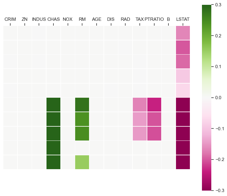
(a) Logistic regression

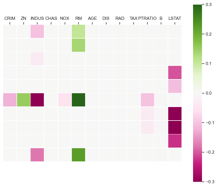
(b) Random forest

Figure 1: Counterfactual explanations for instances $\bm{x}_{i}^{0}$ in Table 3 for two classifiers, the logistic regression and the random forest. The explanations have been calculated solving model (CEsep) with $C_{i}(\bm{x}_{i}^{0},\bm{x}_{i})=\|\bm{x}^{0}_{i}-\bm{x}_{i}\|_{2}^{2}+\lambda_{ind}\|\bm{x}_{i}^{0}-\bm{x}_{i}\|_{0}$ for $\lambda_{ind}=0.02$. The feature perturbations are displayed.

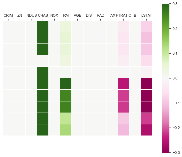
(a) Logistic regression

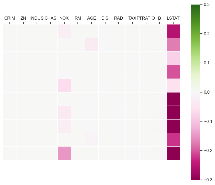
(b) Random forest

Figure 2: Counterfactual explanations for instances $\bm{x}_{i}^{0}$ in Table 3 for two classifiers, the logistic regression and the random forest. The explanations have been calculated solving models (ColCELR) and (ColCEATM) with cost function (1) with $\lambda_{ind}=0$, $\lambda_{glob}=0.2$. The feature perturbations are displayed.

It is worth noting how much sense the counterfactuals shown in the different heatmaps make. As one should expect, to increase the value of a house, i.e., change from the negative to the positive class, the counterfactual explanation shows us that the number of rooms (RM) must increase and the % lower status of the population (LSTAT) has to decrease.

Also, comparing the changes in the separable case (Figure 1) with the non-separable case (Figure 2) one must change 5 and 7 features globally in the separable case in the logistic regression case and the Random Forest case respectively, whereas it is reduced to 4 and 3 features in the non-separable case.

Looking at the results, it can be seen that the features LSTAT, RM, CHAS and PTRATIO are the features that have the greatest impact on changing the instances from the negative to the positive class for this group of instances and the logistic regression model. For the Random Forest, the critical features are NOX, AGE and LSTAT.

Secondly, we will display for all the instances in the Boston housing dataset that were classified in the negative class by the logistic regression model, i.e. that comply with

$$\bm{w}\bm{x}_{i}^{0}+b<0,\quad\forall i=1,\dots,I,$$ (23)

the key features that globally would need to change in order to change its class. We consider $I^{*}=I$ and $\nu=0$. To obtain the Pareto front, we will consider the global sparsity term as a hard constraint, instead of in the objective function. Thus, instead of solving (ColCELR), we will consider the following optimization problem:

$$\begin{split}\min_{\underline{\bm{x}},\bm{y},\bm{\xi},\bm{\xi^{*}},\bm{u}}\quad&\sum_{i=1}^{I}\|\bm{x}_{i}^{0}-\bm{x}\|_{2}^{2}\\ \text{s.t.}\quad&\sum_{j=1}^{J}\xi^{*}_{j}\leq F_{\text{max}}\\ &\eqref{eq:cons_plaus},\eqref{eq:l0i},\eqref{eq:l0i2}\\ &\eqref{eq:l0g1},\eqref{eq:l0g2},\eqref{eq:cons_i22}-\eqref{eq:fortet5}.\end{split}$$ (ColCELRhard)

To describe the Pareto front, we solve this problem for all the possible values of the global sparsity that one can reach, i.e., when $F_{\text{max}}$ takes values 2 to 13. Note that for $F_{\text{max}}=1$, the optimization problem is infeasible. The features that are changed are displayed in Figure 3. In this case, we can see a smooth transition in the increase of the perturbed features.

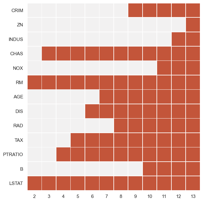
Figure 3: Features that need to be perturbed (in red) for all the instances in the Boston housing dataset that comply with (23) when solving Problem (ColCELRhard) for all the values of $F_{\text{max}}$ to describe the Pareto front. The classifier considered is a logistic regression model. $F_{\text{max}}=1$ yields an infeasible problem.

Thirdly, we look at $\mathcal{I}^{*}$, which can detect outliers from a group. Considering the same group as before, i.e., the instances that meet condition (23), we calculate the counterfactual explanations for 95% of them, leaving 5%. We do this for cost function (1) with $\lambda_{ind}=0$ and two values of $\lambda_{glob}=0.1,10$. The counterfactuals can be seen in Figure 4.

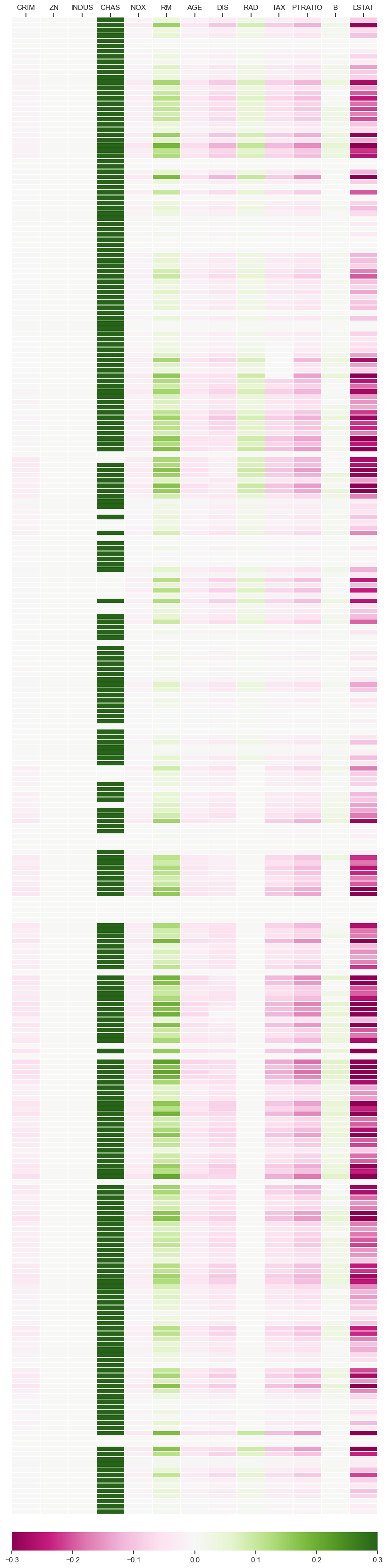
(a) $\lambda_{glob}=0.1$

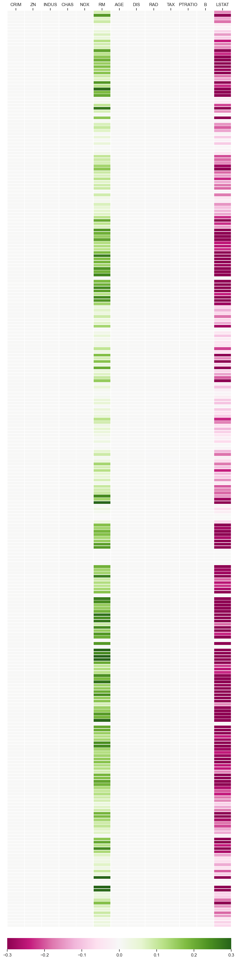
(b) $\lambda_{glob}=10$

Figure 4: Counterfactual explanations for all the instances in the Boston housing dataset that comply with (23). The classifier considered is a logistic regression model. The explanations have been calculated solving model (ColCELR) with $\lambda_{ind}=0$, $\lambda_{glob}=0.1$ (left), $10$ (right), and $I^{*}=\lceil 0.95I\rceil$. The feature perturbations are displayed.

In this case, for both values of $\lambda_{glob}=0.1,10$ considered the same outliers are outlined. The index of the outliers, i.e., the instances that are not perturbed and therefore do not have a counterfactual associated, are 141, 373, 374, 384, 385, 386, 387, 388, 398, 412, 414, 438, 489, 490.

4 Conclusions

In this paper, a unified approach is proposed to build collective counterfactual explanations in classification problems by means of mathematical optimization: minimal cost perturbations on the instances in a group of interest are sought so that, after being perturbed, such instances are classified by the classifier in the desired class. Perturbations costs are modeled taking into account both the magnitude of the change and also the number of predictor variables that need to be changed, either individually or globally. The model is expressed as a mathematical optimization problem, detailed for the case of a linear classifier (as e.g. in logistic regression or linear SVMs) and for additive trees (as e.g.  in random forests or XGBoost). We have illustrated our methodology on several real-world datasets.

There are several interesting lines of future research. First, in our numerical illustrations we have certified that all optimization problems have been solved to optimality. However, for problems with a larger number of individuals or a more complex classifier (e.g. a random forest with a large number of trees, or a neural network), it is worthwhile and necessary to investigate more efficient formulations and heuristic algorithms. Second, an extension to our deterministic approach is required when the features measured for instance $\bm{x}^{0}$ are affected by uncertainty, and thus we have not got any more precise values $\bm{x}^{0}$ but some sort of uncertainty sets (Bertsimas et al., 2011). Third, one could have available, instead of a single classification model, a full collection of classifiers, and seek then for a counterfactual explanation leading to the desired change in class assignment in all (or in at least a fraction $\alpha$) of the classifiers, yielding thus a robust counterfactual explanation. Additionally, we are interested in studying the problem for other classifiers, like support vector machine models with non-linear kernels (Carrizosa and Romero Morales, 2013) or optimal randomized classification trees (Blanquero et al., 2020). Finally, we have assumed that we can perturb independently the different features not affecting the remaining ones, but, if available, the set $\mathcal{\underline{X}}^{0}$ could be enriched with causal constraints (Pearl, 2009), so that the perturbation of a feature is restricted by the those of features correlated with it. Accommodating causality in our models is a challenge which deserves further analysis.

Appendix

A Formulation for ATM

Consider the case where the classifier is an ATM with $T$ trees. For an instance $\bm{x}_{i}$, tree $t\in\{1,\dots,T\}$ predicts, with weight $w^{t}\geq 0$, the positive or negative class. Then, $\bm{x}_{i}$ is allocated to the class for which the overall weight of the trees classifying $\bm{x}_{i}$ in such class is maximal. An ATM can be viewed as a classifier based on scores, where the score $f$ is the sum of the weights associated with trees that classify $\bm{x}_{i}$ in the positive class. More precisely, if $\mathcal{T}_{+}(\bm{x}_{i})$ denotes the subset of trees that classify $\bm{x}_{i}$ in the positive class, then the score function is defined as:

$$f(\bm{x}_{i})=\sum_{t\in\{1,\dots,T\}:t\in\mathcal{T}_{+}(\bm{x}_{i})}w^{t}.$$ (24)

The following notation and decision variables will be used:

Data

$\mathcal{L}^{t}_{k}$	subset of leaves in tree $t$ whose output is class $k=1,\dots,K$, $t=1,\dots,T$
$\mathcal{L}^{t}$	set of leaves in tree $t$. Hence, $\mathcal{L}^{t}=\cup_{k}\mathcal{L}^{t}_{k}$, $t=1,\dots,T$
$\text{Left}(l,t)$	set of ancestor nodes of leaf $l$ in tree $t$ whose left branch takes part in the path that ends in $l$, $l\in\mathcal{L}^{t}$, $t=1,\dots,T$
$\text{Right}(l,t)$	set of ancestor nodes of leaf $l$ in tree $t$ whose right branch takes part in the path that ends in $l$, $l\in\mathcal{L}^{t}$, $t=1,\dots,T$
$v(s)$	feature used in split $s$, $s\in\text{Left}(l,t)\cup\text{Right}(l,t)$
$c_{s}$	threshold value used for split $s$, $s\in\text{Left}(l,t)\cup\text{Right}(l,t)$
$w^{t}$	weight of each tree, $t$, $t=1,\dots,T$

Decision Variables

$\bm{\underline{x}}$	counterfactual, $\bm{\underline{x}}\in\mathcal{\underline{X}}^{0}$
$z_{i,l}^{t}$	binary decision variable that indicates whether the counterfactual instance $i$ ends in leaf $l\in\mathcal{L}^{t}$ ($z_{i,l}^{t}=1$) or not ($z_{i,l}^{t}=0$), $t=1,\dots,T$

Since the structure of the ATM is given, i.e., the topology of the trees, the splits, and the thresholds used in each of the trees, the only decision variables are those defined to indicate in which leaf the counterfactual $\bm{x}_{i}$ ends. Once we know in which path the solution is, the branching condition is determined as well. For each split $s\in\text{Left}(l,t)$ the condition is true, $x_{iv(s)}\leq c_{s}$. Similarly, for each split $s\in\text{Right}(l,t)$ the condition is false, then $x_{iv(s)}>c_{s}$.

The branching conditions are only activated if we end in the corresponding leaf. We introduce these logical conditions using the big $M$-method:

$$x_{iv(s)}-M_{1}(1-z_{i,l}^{t})+\epsilon\leq c_{s}\quad s\in\text{Left}(l,t)$$ (25)

$$x_{iv(s)}+M_{2}(1-z_{i,l}^{t})-\epsilon\geq c_{s}\quad s\in\text{Right}(l,t).$$ (26)

Since a strict inequality is not supported by Mixed-Integer Optimization solvers, following Bertsimas and Dunn [2017], we have introduced a small constant $\epsilon$ in (25) and (26) and changed the inequality to non-strict. With this definition, we are not allowing our variable $x_{iv(s)}$ to take values around the threshold value $c_{s}$ at the split $s$.

Please note that the value of $M_{1}$ and $M_{2}$ can be tightened for each split. Assuming all features $j$ are bounded and that the lower and upper bounds are known, i.e., $lb_{j}\leq x_{ij}\leq ub_{j}$, $j=1,\dots,J$ $i=1\dots,I$, one can take as big $M$ the following values:

$$M_{1}= \max\{|lb_{v(s)}|,|ub_{v(s)}|\}-c_{s}$$ (27)

$$M_{2}= \min\{|lb_{v(s)}|,|ub_{v(s)}|\}+c_{s}+\epsilon.$$ (28)

Moreover, for the dummies of the categorical variables, we can assume that $\epsilon=0$.

Using the decision variables $z_{i,l}^{t}$ associated with the counterfactual $\bm{x}_{i}$, we can write the score function as a linear function:

$$f(\bm{x}_{i})=\sum_{t=1}^{T}\sum_{l\in\mathcal{L}^{t}_{k}}w^{t}z_{i,l}^{t}.$$

As before, we will consider the parametrized family of cost functions $C$ in (1). The formulation for Problem (ColCE) for ATM with this cost function yields as follows:

$$\min_{\underline{\bm{x}},\bm{y},\bm{z},\bm{\xi},\bm{\xi^{*}}}\quad \sum_{i=1}^{I}\|\bm{x}_{i}^{0}-\bm{x}\|_{2}^{2}+\lambda_{ind}\sum_{i=1}^{I}\sum_{j=1}^{J}\xi_{ij}+\lambda_{glob}\sum_{j=1}^{J}\xi^{*}_{j}$$ (29)

s.t. $$x_{iv(s)}-M_{1}(1-z_{i,l}^{t})+\epsilon\leq c_{s}\quad\forall s\in\text{Left}(l,t)\quad\forall l\in\mathcal{L}^{t}\quad t=1,\dots,T\quad i=1\dots,I$$ (30)

$$x_{iv(s)}+M_{2}(1-z_{i,l}^{t})-\epsilon\geq c_{s}\quad\forall s\in\text{Right}(l,t)\quad\forall l\in\mathcal{L}^{t}\quad t=1,\dots,T\quad i=1\dots,I$$ (31)

$$\sum_{l\in\mathcal{L}^{t}}z_{i,l}^{t}=1\quad t=1,\dots,T\quad i=1,\dots,I$$ (32)

$$\sum_{t=1}^{T}\sum_{l\in\mathcal{L}^{t}_{+}}w^{t}z_{i,l}^{t}y_{i}\geq\nu y_{i}\quad i=1,\dots,I$$ (33)

$$\sum_{i=1}^{I}y_{i}=I^{*}$$ (34)

$$z_{i,l}^{t}\in\{0,1\}\quad\forall l\in\mathcal{L}^{t}\quad t=1,\dots,T\quad i=1,\dots,I$$ (35)

$$y_{i}\in\{0,1\}\quad i=1,\dots,I$$ (36)

$$\underline{\bm{x}}\in\underline{\mathcal{X}}^{0}$$ (37)

$$\eqref{eq:l0i}-\eqref{eq:l0i2},\eqref{eq:l0g1}-\eqref{eq:l0g2}.$$

Constraints (30) and (31) determine where the counterfactual instance ends and constraint (32) enforces that only one leaf is active for each tree. Constraint (33) enforces that the counterfactual instance is classified in the positive class if it belongs to $\mathcal{I^{*}}$. With constraint (34) the number of individuals to be changed is imposed. Constraint (35) and (36) ensure that each $z_{i,l}^{t}$ and $y_{i}$ is binary, and constraint $\eqref{eq:rf13g}$ that the counterfactuals $\bm{\underline{x}}$ are in the feasible set $\mathcal{\underline{X}}^{0}$. Constraints (8)-(9), (11)-(12) are as for Problem (ColCELR).

One can also linearize constraint (33) using again the Fortet linearization technique. Introducing a new binary decision variable $u_{i,l}^{t}\in\{0,1\}$. Instead of (33), the following constraints are added to our model:

$$\sum_{t=1}^{T}w^{t}\sum_{l\in\mathcal{L}^{t}_{+}}u_{i,l}\geq\nu y_{i}\qquad i=1,\dots,I$$ (38)

$$u_{i,l}^{t}\leq y_{i}\qquad i=1,\dots,I,\quad l\in\mathcal{L}^{t}_{k}\quad t=1,\dots,T$$ (39)

$$u_{i,l}^{t}\leq z_{i,l}^{t}\qquad i=1,\dots,I\quad l\in\mathcal{L}_{k}^{t}\quad t=1,\dots,T$$ (40)

$$u_{i,l}^{t}\geq y_{i}+z_{i,l}^{t}-1\qquad i=1,\dots,I\quad l\in\mathcal{L}_{k}^{t}\quad t=1,\dots,T$$ (41)

$$u_{i,l}^{t}\in\{0,1\}\qquad i=1,\dots,I,\quad l\in\mathcal{L}_{k}^{t}\quad t=1,\dots,T.$$ (42)

The final formulation is as follows:

$$\begin{split}\min_{\underline{\bm{x}},\bm{y},\bm{z},\bm{\xi},\bm{\xi^{*}},\bm{u}}\quad&\sum_{i=1}^{I}\|\bm{x}_{i}^{0}-\bm{x}\|_{2}^{2}+\lambda_{ind}\sum_{i=1}^{I}\sum_{j=1}^{J}\xi_{ij}+\lambda_{glob}\sum_{j=1}^{J}\xi^{*}_{j}\\ \text{s.t.}\quad&\eqref{eq:l0i}-\eqref{eq:l0i2},\eqref{eq:l0g1}-\eqref{eq:l0g2}\\ &\eqref{eq:rf1g}-\eqref{eq:rf6g},\eqref{eq:rfi}-\eqref{eq:fort5}.\end{split}$$ (ColCEATM)

We obtain a Mixed Integer Convex Quadratic Model with linear constraints.

Supplementary material for ‘‘Generating Collective Counterfactual Explanations in Score-Based Classification via Mathematical Optimization"

The same experiments described in Section 3 of the main paper for the Boston Housing dataset have been carried out in 3 additional datasets. Table 1 of the main paper reports their name, source of origin, number of instances, number of total features and their type. The source code and the data to reproduce all results are available at https://github.com/jasoneramirez/CollectiveCE.

In these datasets, there are some nominal categorical features that have been transformed into numerical ones using the standard one-hot encoding, with one dummy variable for each category. Therefore, in the heatmaps each category is represented. However, one must take into account that a change from one category to another, although visualized as two dummy variables changes in the heatmaps (one is activated and changes from 1 to 0, whereas another is deactivated and goes from 0 to 1), in reality only one categorical feature is being perturbed.

COMPAS

The COMPAS dataset was collected by ProPublica [Angwin et al., 2019] as part of their analysis on recidivism decisions in the United States. Following Karimi et al. [2020], Mothilal et al. [2020], Parmentier and Vidal [2021], 5 features are considered. The description of the dataset is detailed in Table 3.

Variable	Definition	Type
Race	race of defendants: African-American, Asian, Caucasian, Hispanic, Native American, Other	categorical (nominal)
AgeGroup	age category of defendants: 1 ($<$25), 2 (25-45), 3 ($>$45)	categorical (ordinal)
Sex	sex of defendants: 0 (male) or 1 (female)	binary
PriorsCount	prior criminal records of defendants	numerical
ChargeDegree	charge degree of defendants: 0 (Misdemeanor), 1 (Felony)	binary
TwoYearRecid	binary variable indicate whether defendant is rearrested at within two years: 1 (no), -1 (yes)	target

Table 3: Description of the features used of the COMPAS dataset

We will conduct the same experiments done for the Boston housing dataset. First, counterfactual explanations for 10 individuals that were classified originally in the negative class by both classifiers, logistic regression and random forest, are calculated. The original values of the 10 instances can be seen in Table 4.

Race	AgeGroup	Sex	PriorsCount	ChargeDegree
African-American	2	0	7	1
African-American	2	0	16	1
African-American	2	0	18	1
African-American	1	0	3	1
African-American	1	0	1	1
African-American	1	0	3	1
Caucasian	3	0	28	1
African-American	3	0	38	1
Caucasian	3	1	28	1
African-American	2	0	19	1

Table 4: Feature values of $\bm{\underline{x}}^{0}=(\bm{x}^{0}_{1},\dots,\bm{x}^{0}_{10})$ used for the models in Figures 5-6.

We solve models (CEsep), (ColCELR) and (ColCEATM), considering different combinations of the values of $\lambda_{ind}$ and $\lambda_{glob}$.

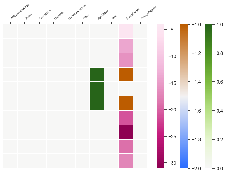
(a) Logistic regression

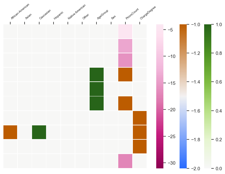
(b) Random forest

Figure 5: Counterfactual explanations for instances $\bm{x}_{i}^{0}$ in Table 4 for two classifiers, the logistic regression and the random forest. The explanations have been calculated solving model (CEsep) with $C_{i}(\bm{x}_{i}^{0},\bm{x}_{i})=\|\bm{x}^{0}_{i}-\bm{x}_{i}\|_{2}^{2}+\lambda_{ind}\|\bm{x}_{i}^{0}-\bm{x}_{i}\|_{0}$ for $\lambda_{ind}=0.02$. The feature perturbations are displayed.

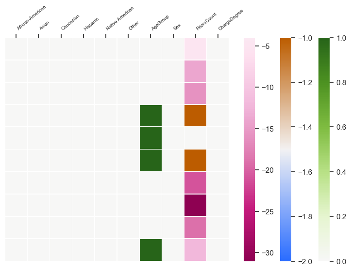
(a) Logistic regression

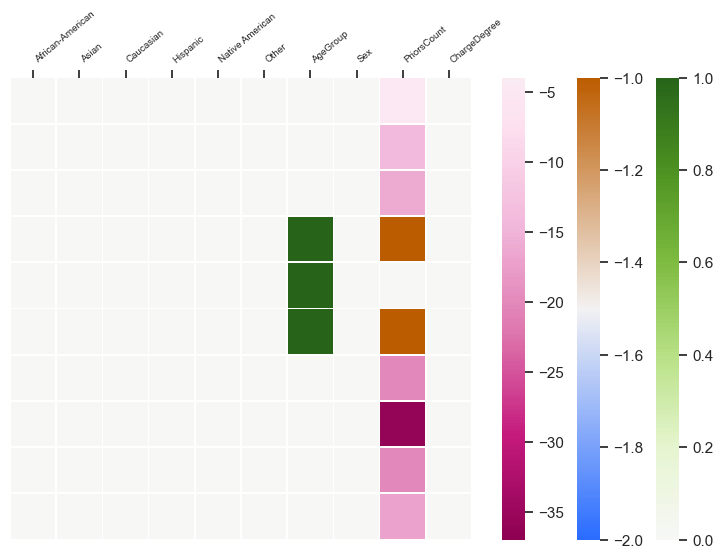
(b) Random forest

Figure 6: Counterfactual explanations for instances $\bm{x}_{i}^{0}$ in Table 4 for two classifiers, the logistic regression and the random forest. The explanations have been calculated solving models (ColCELR) and (ColCEATM) with cost function (1) with $\lambda_{ind}=0$, $\lambda_{glob}=0.2$. The feature perturbations are displayed.

For this dataset, the counterfactuals obtained also make sense. As one should expect, to not be labeled as reincident, the number of prior criminal records has to decrease as well as the charge degree. Also, the COMPAS dataset has been used to exemplify unfairness in classification. This can be detected, in the separable case, for the Random Forest. Indeed, for one instance, if we were allowed to change their race from African-American to Caucasian, decreasing their charge degree would result in a positive classification.

Comparing the results in the separable case (Figure 5) with the non-separable case (Figure 6) we see that 4 features need to be changed globally (i.e., Race, AgeGroup, PriorsCount and ChargeDegree) in the separable case in the Random Forest case, whereas only 2 features need to be changed (AgeGroup and PriorsCount) in the non-separable case. For the logistic regression case, the perturbed features are the same in the separable and non-separable cases.

Looking at the results, it can be seen that the features AgeGroup and PriorsCount are the features that have the greatest impact on changing the instances from the negative to the positive class for this group of instances and for both models. It is worth noticing that previous work [Dressel and Farid, 2018] about this dataset reached the conclusion that despite having the original dataset a collection of 137 features, the same accuracy could be achieved with a simple linear classifier with only two features. These two features where the age and the priors counts.

Next, we display for all the instances in the COMPAS dataset that were classified in the negative class by the logistic regression model, i.e. that comply with (23), the key features that globally would need to be modified in order to change its class. We solve Problem (ColCELRhard) for $F_{\text{max}}=1,2,3,4,5$. For $F_{\text{max}}=1$, the optimization problem is infeasible. For the rest of the values of $F_{m}ax$, the features that are changed are displayed in Figure 7.

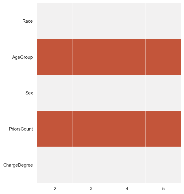
Figure 7: Features that need to be perturbed (in red) for all the instances in the COMPAS dataset that comply with (23) when solving Problem (ColCELRhard) for all the values of $F_{\text{max}}$ to describe the Pareto front. The classifier considered is a logistic regression model. $F_{\text{max}}=1$ yields an infeasible problem.

We reach the same conclusion as before: the only critical features to change the predicted class are AgeGroup and PriorsCount.

Finally, for this dataset, we look at $\mathcal{I}^{*}$, which can detect outliers from a group. The counterfactuals can be seen in Figure 8.

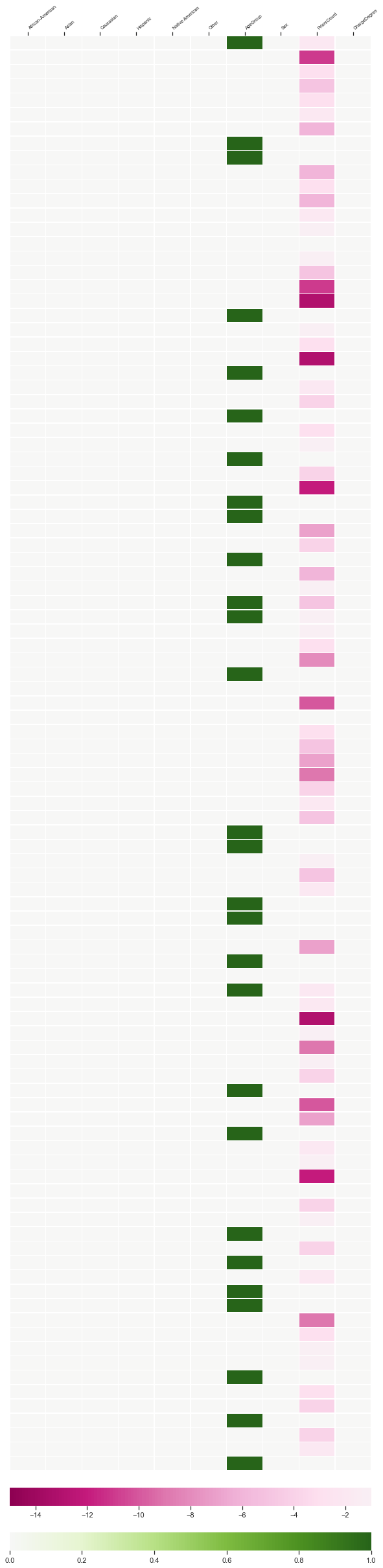
(a) $\lambda_{glob}=0.1$

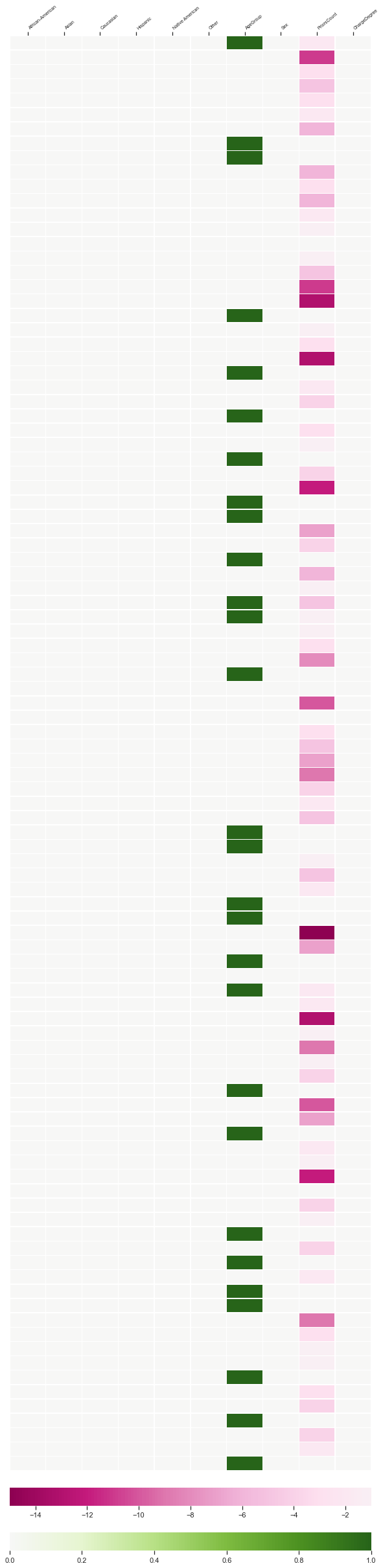
(b) $\lambda_{glob}=10$

Figure 8: Visualization of 100 of the counterfactual explanations for all the instances in the COMPAS dataset that comply with (23). The classifier considered is a logistic regression model. The explanations have been calculated solving model (ColCELR) with $\lambda_{ind}=0$, $\lambda_{glob}=0.1$ (left), $10$ (right), and $I^{*}=\lceil 0.95I\rceil$. The feature perturbations are displayed.

For both values of lambda, the two features that are perturbed are the same. We obtain two optimal sets of outliers with the same total euclidean distance between the original samples and the counterfactuals.

Credit

The Credit dataset [Yeh and Lien, 2009] was used to predict the probability of default payments in Taiwan. The data was preprocessed as in Karimi et al. [2020], Parmentier and Vidal [2021]. The description of the dataset is detailed in Table 5.

Variable	Definition	Type
isMale	sex of individual: 0 (female), 1(male)	binary
isMarried	marital status: 0 (not married), 1 (married)	binary
AgeGroup	age category: 1 ($<$25), 2 (25-39), 3 (40-59), 4 ($\geq$60)	categorical (ordinal)
EducationLevel	education level: 1 (other), 2 (highschool), 3 (university), 4 (graduate)	categorical (ordinal)
MaxBillAmountOverLast6Months	maximum bill amount over the last 6 months	numerical
MaxPaymentAmountOverLast6Months	maximum payment amount over the last 6 months	numerical
MonthsWithZeroBalanceOverLast6Months	months with zero balance over the last 6 months	numerical
MonthsWithLowSpendingOverLast6Months	months with low spending (bill$<$0.2) over last 6 months	numerical
MonthsWithHighSpendingOverLast6Months	months with high spending (bill$>$0.8) over last 6 months	numerical
MostRecentBillAmount	most recent bill amount	numerical
MostRecentPaymentAmount	most recent payment amount	numerical
TotalOverdueCounts	total overdue counts	numerical
TotalMonthsOverdue	total months overdue	numerical
HasHistoryOfOverduePayments	binary variable indicating whethere the individual has a history of overdue payment: yes(1), no (0)	binary
NoDefaultNextMonth	binary variable indicating whether the individual will default next month (0) or not (1)	target

Table 5: Description of the features of the Credit dataset

First, counterfactual explanations for 10 individuals that were classified originally in the negative class by both classifiers, are calculated. The original values of these 10 instances can be seen in Table 6.

isMale	isMarried	AgeGroup	EducationLevel	MaxBillAmountOverLast6Months	MaxPaymentAmountOverLast6Months	MonthsWithZeroBalanceOverLast6Months	MonthsWithLowSpendingOverLast6Months	MonthsWithHighSpendingOverLast6Months	MostRecentBillAmount	MostRecentPaymentAmount	TotalOverdueCounts	TotalMonthsOverdue	HasHistoryOfOverduePayments
1	1	3	4	0.1704	0.0107	0	0	6	0.2659	0.0357	1	22	1
1	0	2	3	0.0632	0.0119	0	0	5	0.0754	0.0396	1	32	1
1	0	2	2	0.1431	0.0169	0	0	6	0.2217	0.0201	1	12	1
0	1	2	4	0.2153	0.0095	0	0	6	0.3341	0.0318	1	12	1
1	0	2	4	0.1724	0.0072	0	0	6	0.2832	0.0240	2	8	1
1	1	3	4	0.0811	0.0087	0	0	5	0.1175	0.0292	2	8	1
1	0	2	4	0.1079	0.0089	0	0	5	0.1623	0.0298	1	12	1
1	1	3	2	0.1559	0.0086	0	0	6	0.2689	0.0220	1	12	1
1	0	2	4	0.1071	0.0086	0	0	6	0.1599	0.0285	1	8	1
1	0	2	3	0.1785	0.0078	0	0	6	0.2958	0.0259	1	12	1

Table 6: Feature values of $\bm{\underline{x}}^{0}=(\bm{x}^{0}_{1},\dots,\bm{x}^{0}_{10})$ used for the models in Figures 9--10.

We solve models (CEsep), (ColCELR) and (ColCEATM), considering different combinations of the values of $\lambda_{ind}$ and $\lambda_{glob}$.

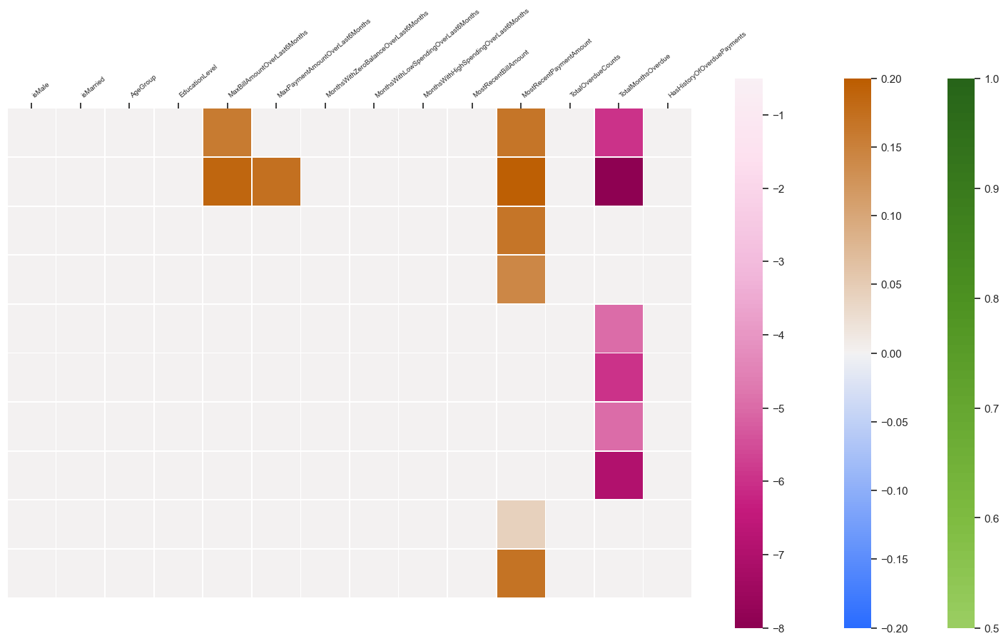
(a) Logistic regression

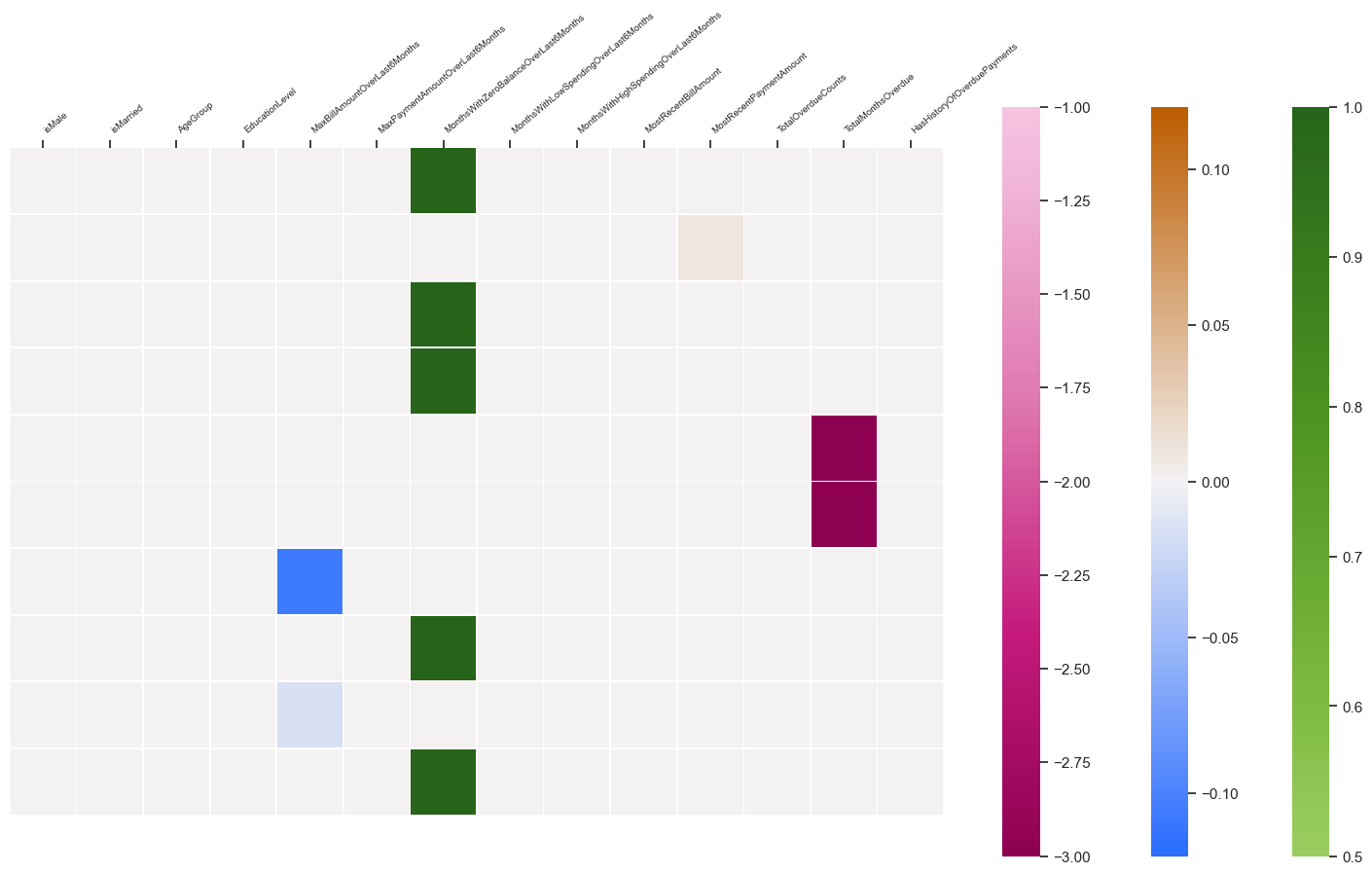
(b) Random forest

Figure 9: Counterfactual explanations for instances $\bm{x}_{i}^{0}$ in Table 6 for two classifiers, the logistic regression and the random forest. The explanations have been calculated solving model (CEsep) with $C_{i}(\bm{x}_{i}^{0},\bm{x}_{i})=\|\bm{x}^{0}_{i}-\bm{x}_{i}\|_{2}^{2}+\lambda_{ind}\|\bm{x}_{i}^{0}-\bm{x}_{i}\|_{0}$ for $\lambda_{ind}=0.02$. The feature perturbations are displayed.

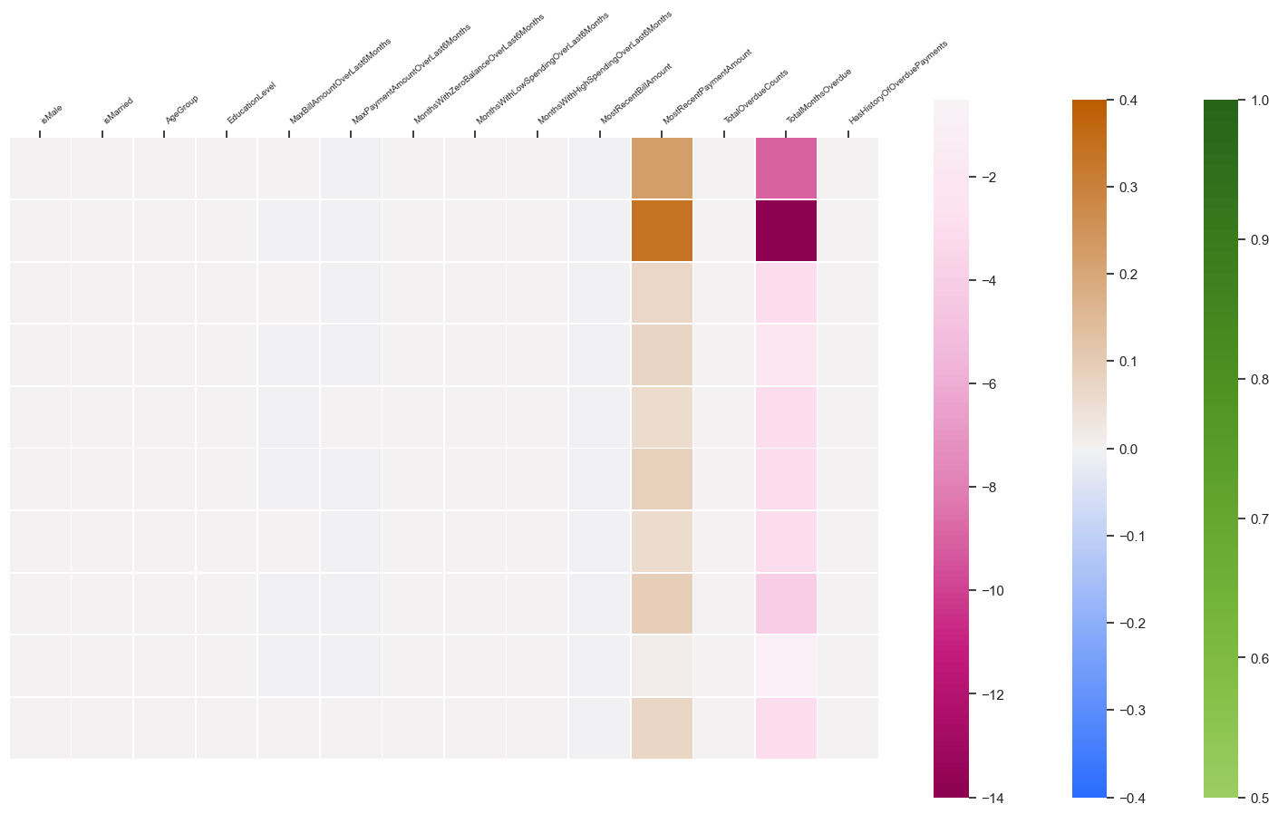
(a) Logistic regression

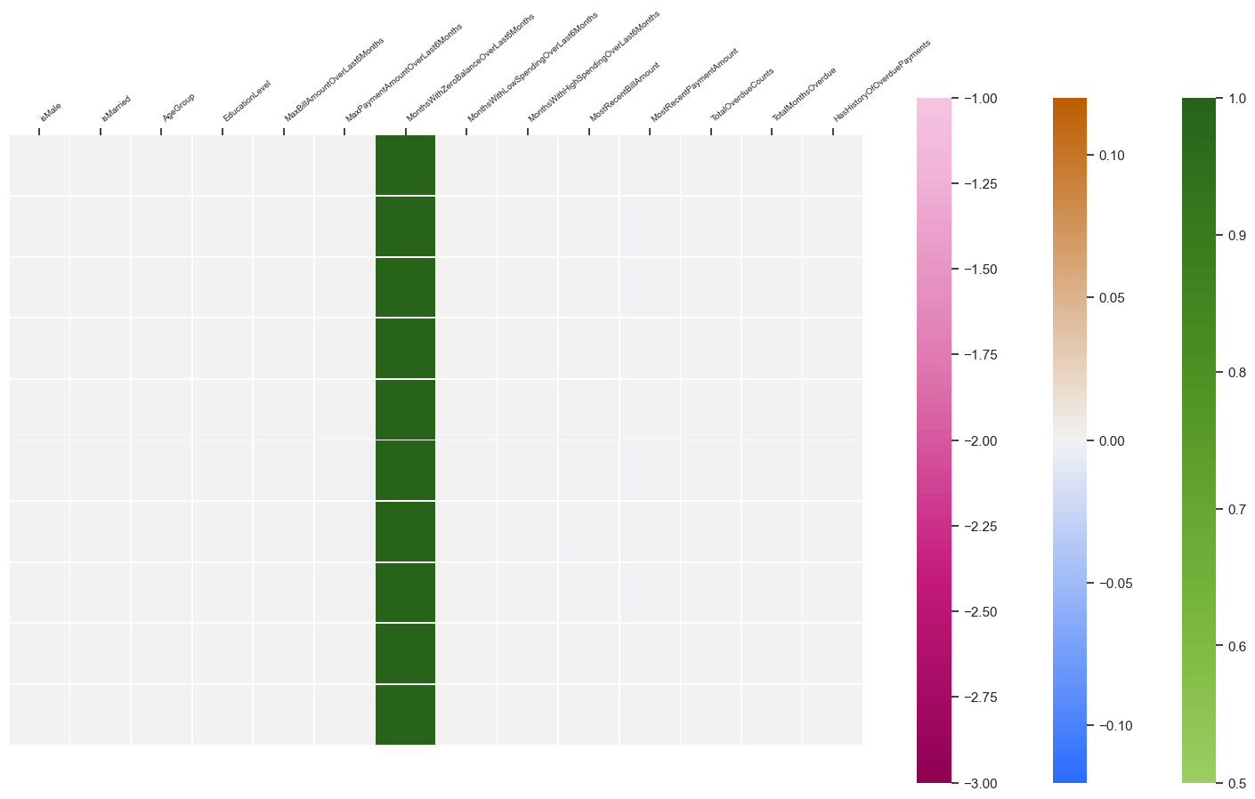
(b) Random forest

Figure 10: Counterfactual explanations for instances $\bm{x}_{i}^{0}$ in Table 6 for two classifiers, the logistic regression and the random forest. The explanations have been calculated solving models (ColCELR) and (ColCEATM) with cost function (1) with $\lambda_{ind}=0$, $\lambda_{glob}=0.2$. The feature perturbations are displayed.

For this dataset, to not be labeled as default, the number of total months overdue and the most recent payment amount has to decrease, whereas the number of months with zero balance has to increase.

Comparing the changes in the separable case (Figure 9) with the non-separable case (Figure 10), we can see a big difference on the number of features needed to be perturbed. We see that one must change 4 features globally in the separable case, both in the logistic regression and random forest case, whereas it is reduced to 2 and 1 feature in the non-separable case, respectively.

Looking at the results, it can be seen that the critical features are different for each classifier for these 10 instances. For the logistic regression, the features that have the greatest impact are MostRecentPayment and TotalMonthsOverdue, whereas for the random forest is the feature about the number of months with zero balance over the last 6 months.

Next, we display for all the instances in the Credit dataset that comply with (23), the key features that globally would need to to be modified in order to change its class. We solve Problem (ColCELRhard) for the different values of $F_{\text{max}}$ from 1 to 14. The features changed are displayed in Figure 11.

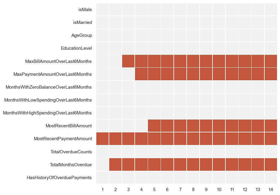
Figure 11: Features that need to be perturbed (in red) for all the instances in the Credit dataset that comply with (23) when solving Problem (ColCELRhard) for all the values of $F_{\text{max}}$ to describe the Pareto front. The classifier considered is a logistic regression model.

We can see that the maximum number of features needed to change the prediction are 5.

Finally, for this dataset, we look at $\mathcal{I}^{*}$, which can detect outliers from a group. The counterfactuals can be seen in Figure 12.

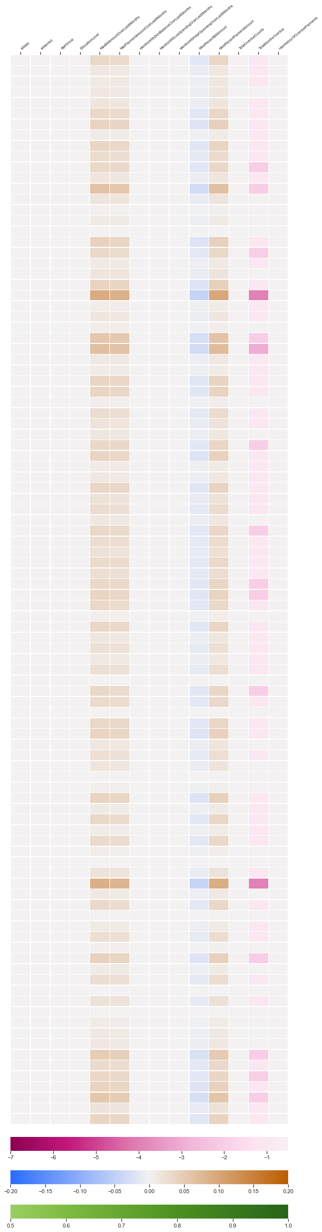
(a) $\lambda_{glob}=0.1$

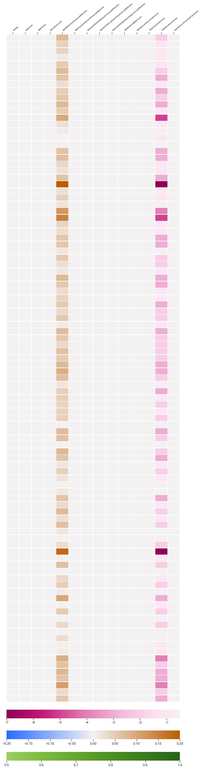
(b) $\lambda_{glob}=10$

Figure 12: Visualization of 100 of the counterfactual explanations for all the instances in the Credit dataset that comply with (23). The classifier considered is a logistic regression model. The explanations have been calculated solving model (ColCELR) with $\lambda_{ind}=0$, $\lambda_{glob}=0.1$ (left), $10$ (right), and $I^{*}=\lceil 0.95I\rceil$. The feature perturbations are displayed.

From the 144 outliers, 113 are in common for both cost functions.

Student’s performance

The Students Performance dataset includes student grades, demographic, social and school related features and aims at predicting whereas a student will pass a course or not. The description of the dataset is detailed in Table 7.

Variable	Definition	Type
school	student’s school: 0 (Gabriel Pereira), 1 (Mousinho da Silveira)	binary
sex	student’s sex: 0 (male), 1 (female)	binary
age	student’s age	numerical
address	student’s home address type: 0 (rural), 1(urbal)	binary
famsize	family size: 0 (less or equal to 3), 1 (greater than 3)	binary
Pstatus	parent’s cohabitation status: 0 (living together), 1 (apart)	binary
Medu	mother’s education: 0 (none), 1 (primary education), 2 (5th to 9th grade), 3 (secondary education), 4 (higher education)	categorical (ordinal)
Fedu	father’s education: 0 (none), 1 (primary education), 2 (5th to 9th grade), 3 (secondary education), 4 (higher education)	categorical (ordinal)
Mjob	mother’s job: ’teacher’, ’health’ care related, civil ’services’ (e.g. administrative or police), ’at_home’ or ’other’	categorical (nominal)
Fjob	father’s job: ’teacher’, ’health’ care related, civil ’services’ (e.g. administrative or police), ’at_home’ or ’other’	categorical (nominal)
reason	reason to choose this school: close to ’home’, school ’reputation’, ’course’ preference or ’other’	categorical (nominal)
guardian	student’s guardian: ’mother’, ’father’ or ’other’	categorical (nominal)
traveltime	home to school travel time: 1 ($<$15 min) , 2 (15 to 30 min), 3 (30 min to 1 hour), 4 ($>$1 hour)	categorical (ordinal)
studytime	weekly study time: 1 ($<$2 hours), 2 (2 to 5 hours), 3 (5 to 10 hours), or 4 ($>$10 hours)	categorical (ordinal)
failures	number of past class failures	numerical
schoolsup	extra educational support: 0 (no), 1 (yes)	binary
famsup	family educational support: 0 (no), 1 (yes)	binary
paid	extra paid classes within the course subject: 0 (no), 1 (yes)	binary
activities	extra-curricular activities: 0 (no), 1 (yes)	binary
nursery	attended nursery school: 0 (no), 1 (yes)	binary
higher	wants to take higher education : 0 (no), 1 (yes)	binary
internet	Internet access at home: 0 (no), 1 (yes)	binary
romantic	with a romantic relationship: 0 (no), 1 (yes)	binary
famrel	quality of family relationships: from 1 (very bad) to 5(excellent)	categorical (ordinal)
freetime	free time after school: from 1 (very low) to 5 (very high)	categorical (ordinal)
goout	going out with friends: from 1 (very low) to 5 (very high)	categorical (ordinal)
Dalc	workday alcohol consumption: from 1 (very low) to 5 (very high)	categorical (ordinal)
Walc	weekend alcohol consumption: from 1 (very low) to 5 (very high)	categorical (ordinal)
health	current health status: : from 1 (very low) to 5 (very high)	categorical (ordinal)
absences	number of school absences	numerical
Class	1 if the student passes the math course, -1 otherwise	target

Table 7: Description of the features of the Students performance dataset

First, counterfactual explanations for 10 individuals that were classified originally in the negative class by both classifiers, are calculated. The original values of these 10 instances can be seen in Table 8.

Mjob	Fjob	reason	guardian	school	sex	age	address	famsize	Pstatus	Medu	Fedu	traveltime	studytime	failures	schoolsup	famsup	paid	activities	nursery	higher	internet	romantic	famrel	freetime	goout	Dalc	Walc	health	absences
services	other	reputation	father	0	1	15	1	1	0	2	1	3	3	0	1	1	1	1	1	1	1	1	5	2	2	1	1	4	4
at_home	other	reputation	mother	0	1	15	0	1	0	2	2	1	1	0	1	1	1	1	1	1	1	1	4	3	1	1	1	2	8
other	at_home	course	father	0	1	16	1	0	0	2	2	2	2	1	1	1	1	1	1	1	1	1	4	3	3	2	2	5	14
other	other	home	mother	0	1	16	1	1	0	2	2	1	2	0	1	1	1	1	1	1	1	1	5	4	4	1	1	5	0
teacher	other	course	mother	0	0	17	1	0	0	4	3	2	2	0	1	1	1	1	1	1	1	1	4	4	4	4	4	4	4
other	other	reputation	mother	0	1	16	1	1	0	2	3	1	2	0	1	1	1	1	1	1	1	1	4	4	3	1	3	4	6
other	other	reputation	mother	0	1	18	0	1	0	3	1	1	2	1	1	1	1	1	1	1	1	1	5	3	3	1	1	4	16
other	other	course	father	0	0	17	1	1	0	2	3	2	1	0	1	1	1	1	1	1	1	1	5	2	2	1	1	2	4
health	other	home	mother	0	1	18	1	0	1	4	4	1	2	0	1	1	1	1	1	1	1	1	4	2	4	1	1	4	14
other	other	course	mother	1	0	18	0	1	0	3	2	2	1	1	1	1	1	1	1	1	1	1	2	5	5	5	5	5	10

Table 8: Feature values of $\bm{\underline{x}}^{0}=(\bm{x}^{0}_{1},\dots,\bm{x}^{0}_{10})$ used for the models in Figures 13--14.

We solve models (CEsep), (ColCELR) and (ColCEATM), considering different combinations of the values of $\lambda_{ind}$ and $\lambda_{glob}$.

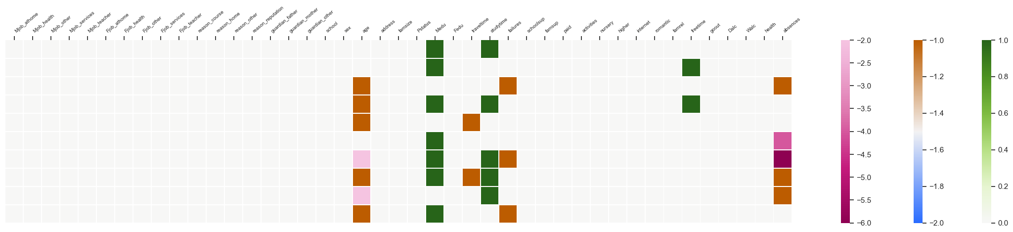
(a) Logistic regression

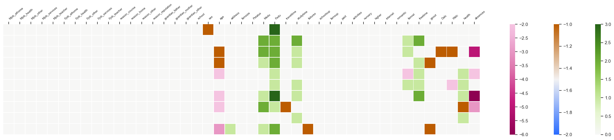
(b) Random forest

Figure 13: Counterfactual explanations for instances $\bm{x}_{i}^{0}$ in Table 8 for two classifiers, the logistic regression and the random forest. The explanations have been calculated solving model (CEsep) with $C_{i}(\bm{x}_{i}^{0},\bm{x}_{i})=\|\bm{x}^{0}_{i}-\bm{x}_{i}\|_{2}^{2}+\lambda_{ind}\|\bm{x}_{i}^{0}-\bm{x}_{i}\|_{0}$ for $\lambda_{ind}=0.02$. The feature perturbations are displayed.

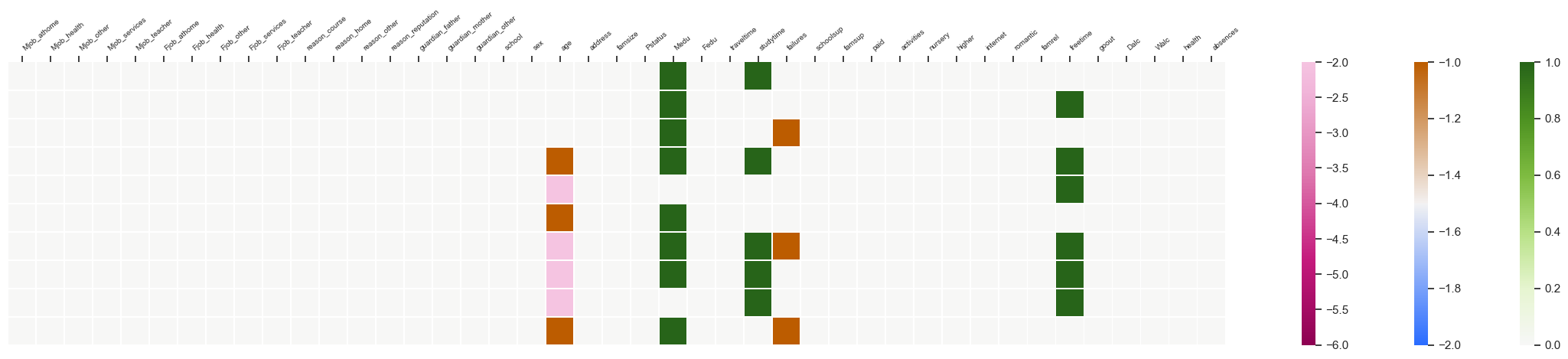
(a) Logistic regression

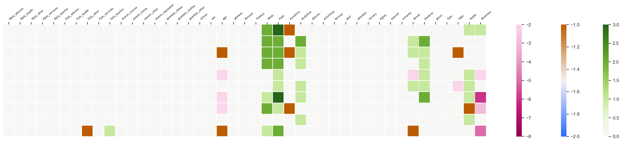
(b) Random forest

Figure 14: Counterfactual explanations for instances $\bm{x}_{i}^{0}$ in Table 8 for two classifiers, the logistic regression and the random forest. The explanations have been calculated solving models (ColCELR) and (ColCEATM) with cost function (1) with $\lambda_{ind}=0$, $\lambda_{glob}=0.2$. The feature perturbations are displayed.

For this dataset, to be classified in the positive class, i.e., passing the course, the features that have to be increased are mostly the mother’s and father’s education, the study time, the free time, the quality of family relations and the health status; whereas the features that have to be mostly decreased are the age, the number of failures, the number of absences, travel time and how much they go out with friends.

Comparing the changes in the separable case (Figure 13) with the non-separable case (Figure 14), one must perturb 7 and 15 features globally in the separable case in the logistic regression and random forest, respectively. This is reduced to 5 and 11 features in the non-separable case.

Focusing in the non-separable case ,we clearly see in the figures that the features that have the greatest impact are the age of the students, the mother’s education, the study time, the number of failures and amount of free time that the students have. In the case of the random forest there seems to be more features that impact on the decision made by the classifiers. Besides the one already mentioned, the father’s education, the health status, the travel time and the number of failures are also perturbed for most records.

Next, we display for all the instances in the Students performance dataset that comply with (23), the key features that globally would need to be perturbed in order to change its class. We solve Problem (ColCELRhard) for different values of the parameter $F_{\text{max}},$ ranging from 1 to 30. For values 1 to 5, the problem was infeasible. The features changed are displayed in Figure 11.

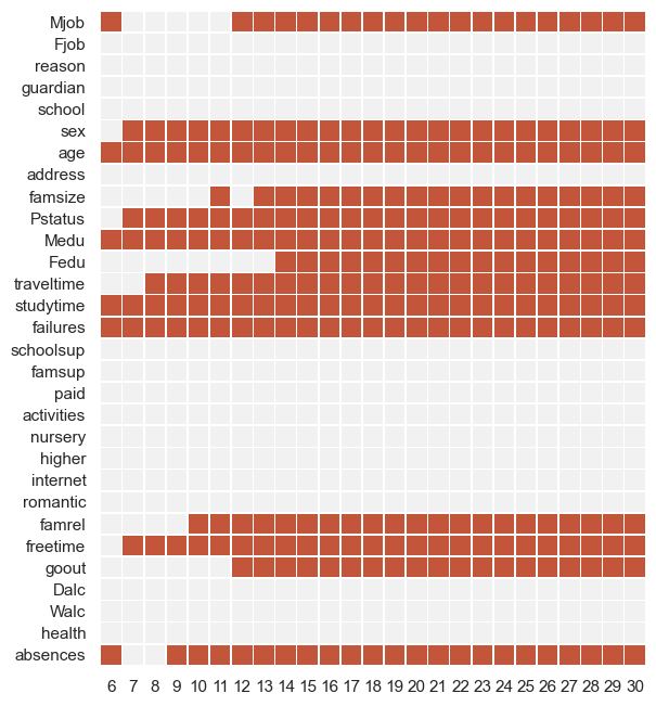
Figure 15: Features that need to be perturbed (in red) for all the instances in the Students performance dataset that comply with (23) when solving Problem (ColCELRhard) for all the values of $F_{\text{max}}$ to describe the Pareto front. The classifier considered is a logistic regression model. $F_{\text{max}}=1,2,3,4,5$ yields an infeasible problem.

We can see that the maximum number of features needed to change the prediction are 14.

Finally, for this dataset, we look at $\mathcal{I}^{*}$, which can detect outliers from a group. The counterfactuals can be seen in Figure 16.

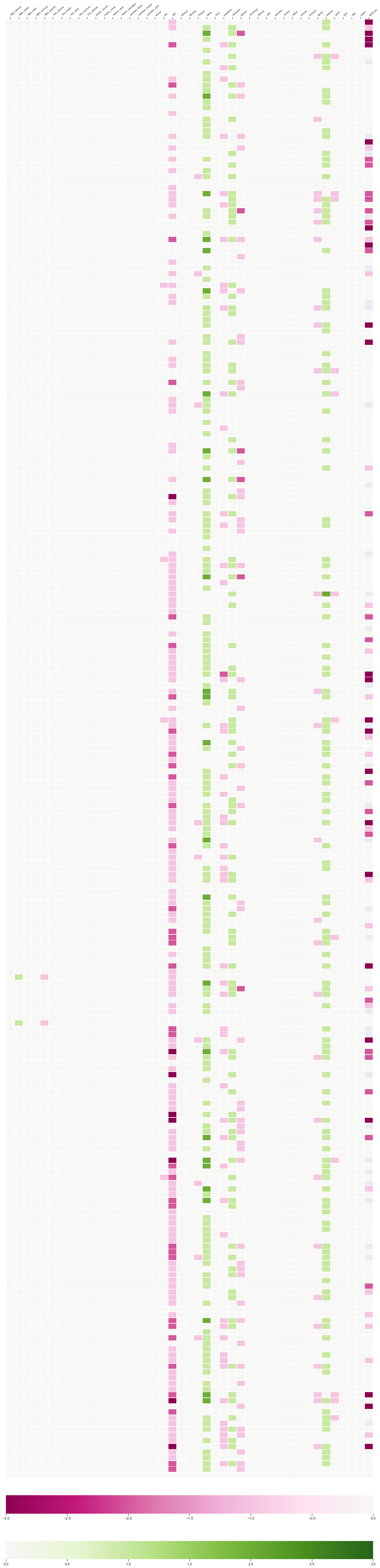
(a) $\lambda_{glob}=0.1$

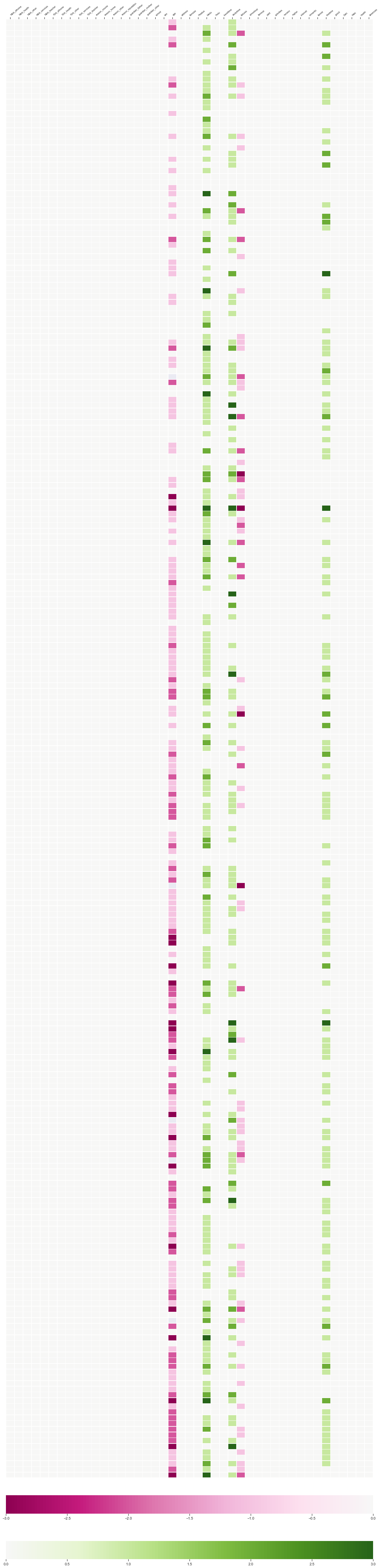
(b) $\lambda_{glob}=10$

Figure 16: Counterfactual explanations for all the instances in the Students performance dataset that comply with (23). The classifier considered is a logistic regression model. The explanations have been calculated solving model (ColCELR) with $\lambda_{ind}=0$, $\lambda_{glob}=0.1$ (left), $10$ (right), and $I^{*}=\lceil 0.95I\rceil$. The feature perturbations are displayed.

For $\lambda_{glob}=0.1$ the indices of the outliers are 28, 57, 62, 69, 79, 85, 91, 121, 151, 174, 198, 225, 254, whereas for $\lambda_{glob}=10$ the indices of the outliers are 27, 28, 31, 46, 50, 122, 124, 140, 146, 167, 174, 202, 216. There are only two in common.

References

- Ahani et al. [2021] N. Ahani, T. Andersson, A. Martinello, A. Teytelboym, and A. C. Trapp. Placement optimization in refugee resettlement. Operations Research, 69:1468--1486, 2021.
- Angwin et al. [2019] J. Angwin, J. Larson, S. Mattu, and L. Kirchner. Machine bias: There’s software used across the country to predict future criminals. and it’s biased against blacks. 2016. URL https://www. propublica. org/article/machine-bias-risk-assessments-in-criminal-sentencing, 2019.
- Benítez-Peña et al. [2021] S. Benítez-Peña, E. Carrizosa, V. Guerrero, M. Dolores Jiménez-Gamero, B. Martín-Barragán, C. Molero-Río, P. Ramírez-Cobo, D. Romero Morales, and M. Remedios Sillero-Denamiel. On sparse ensemble methods: An application to short-term predictions of the evolution of COVID-19. European Journal of Operational Research, 295(2):648--663, 2021.
- Bertsimas and Dunn [2017] D. Bertsimas and J. Dunn. Optimal classification trees. Machine Learning, 106(7):1039--1082, 2017.
- Bertsimas et al. [2011] D. Bertsimas, D.B. Brown, and C. Caramanis. Theory and applications of robust optimization. SIAM Review, 53(3):464--501, 2011.
- Bertsimas et al. [2016] D. Bertsimas, A. King, and R. Mazumder. Best subset selection via a modern optimization lens. The Annals of Statistics, 44(2):813--852, 2016.
- Blanquero et al. [2020] R. Blanquero, E. Carrizosa, C. Molero-Río, and D. Romero Morales. Sparsity in optimal randomized classification trees. European Journal of Operational Research, 284(1):255 -- 272, 2020.
- Boukerche et al. [2020] A. Boukerche, L. Zheng, and O. Alfandi. Outlier detection: Methods, models, and classification. ACM Computing Surveys (CSUR), 53(3):1--37, 2020.
- Browne and Swift [2020] K. Browne and B. Swift. Semantics and explanation: why counterfactual explanations produce adversarial examples in deep neural networks. arXiv preprint arXiv:2012.10076, 2020.
- Brughmans et al. [2023] Dieter Brughmans, Pieter Leyman, and David Martens. Nice: an algorithm for nearest instance counterfactual explanations. Forthcoming in Data Mining and Knowledge Discovery, pages 1--39, 2023.
- Carrizosa and Romero Morales [2013] E. Carrizosa and D. Romero Morales. Supervised classification and mathematical optimization. Computers & Operations Research, 40(1):150--165, 2013.
- [12] E. Carrizosa, M.J. Ramírez Ayerbe, and D. Romero Morales. A new model for counterfactual analysis for functional data. Technical report, IMUS, Sevilla, Spain, https://www.researchgate.net/publication/363539291_A_New_Model_for_Counterfactual_Analysis_for_Functional_Data. Forthcoming in Advances in Data Analysis and Classification.
- Carrizosa et al. [2023] E. Carrizosa, J. Ramírez Ayerbe, and D. Romero Morales. Mathematical optimization modelling for group counterfactual explanations. Technical report, IMUS, Sevilla, Spain, https://www.researchgate.net/publication/368958766_Mathematical_Optimization_Modelling_for_Group_Counterfactual_Explanations, 2023.
- Cui et al. [2015] Z. Cui, W. Chen, Y. He, and Y. Chen. Optimal action extraction for random forests and boosted trees. In Proceedings of the 21th ACM SIGKDD International Conference on Knowledge Discovery and Data Mining, pages 179--188, 2015.
- Dandl et al. [2020] S. Dandl, C. Molnar, M. Binder, and B. Bischl. Multi-objective counterfactual explanations. In International Conference on Parallel Problem Solving from Nature, pages 448--469. Springer, 2020.
- Dhurandhar et al. [2018] A. Dhurandhar, P.-Y. Chen, R. Luss, C.-C. Tu, P. Ting, K. Shanmugam, and P. Das. Explanations based on the missing: Towards contrastive explanations with pertinent negatives. Advances in Neural Information Processing Systems, 31:590--601, 2018.
- Dressel and Farid [2018] Julia Dressel and Hany Farid. The accuracy, fairness, and limits of predicting recidivism. Science Advances, 4(1):eaao5580, 2018.
- Fernández et al. [2020] R.R. Fernández, I.M. de Diego, V. Aceña, A. Fernández-Isabel, and J.M. Moguerza. Random forest explainability using counterfactual sets. Information Fusion, 63:196--207, 2020.
- Fischetti and Jo [2018] M. Fischetti and J. Jo. Deep neural networks and mixed integer linear optimization. Constraints, 23(3):296--309, 2018.
- Fortet [1960] R. Fortet. L’algebre de boole et ses applications en recherche opérationnelle. Trabajos de Estadistica, 11(2):111--118, 1960.
- Freiesleben [2022] T. Freiesleben. The intriguing relation between counterfactual explanations and adversarial examples. Minds and Machines, 32(1):77--109, 2022.
- Guidotti [2022] R. Guidotti. Counterfactual explanations and how to find them: literature review and benchmarking. Forthcoming in Data Mining and Knowledge Discovery, 2022.
- Guidotti et al. [2019] R. Guidotti, A. Monreale, F. Giannotti, D. Pedreschi, S. Ruggieri, and F. Turini. Factual and counterfactual explanations for black box decision making. IEEE Intelligent Systems, 34(6):14--23, 2019.
- Gurobi Optimization [2021] LLC Gurobi Optimization. Gurobi optimizer reference manual, 2021. URL http://www.gurobi.com.
- Harrison Jr and Rubinfeld [1978] D. Harrison Jr and D.L. Rubinfeld. Hedonic housing prices and the demand for clean air. Journal of Environmental Economics and Management, 5(1):81--102, 1978.
- Hart et al. [2011] W. E. Hart, J. Watson, and D. L. Woodruff. Pyomo: modeling and solving mathematical programs in Python. Mathematical Programming Computation, 3(3):219--260, 2011.
- Hart et al. [2017] W. E. Hart, C. D. Laird, J. Watson, D. L. Woodruff, G. A. Hackebeil, B. L. Nicholson, and J. D. Siirola. Pyomo--optimization modeling in Python, volume 67. Springer Science & Business Media, second edition, 2017.
- Hazimeh and Mazumder [2020] H. Hazimeh and R. Mazumder. Fast best subset selection: Coordinate descent and local combinatorial optimization algorithms. Operations Research, 68(5):1517--1537, 2020.
- Joshi et al. [2019] S. Joshi, O. Koyejo, W. Vijitbenjaronk, B. Kim, and J. Ghosh. Towards realistic individual recourse and actionable explanations in black-box decision making systems. arXiv preprint arXiv:1907.09615, 2019.
- Jung et al. [2020] J. Jung, C. Concannon, R. Shroff, S. Goel, and D.G. Goldstein. Simple rules to guide expert classifications. Journal of the Royal Statistical Society: Series A (Statistics in Society), 183(3):771--800, 2020.
- Kanamori et al. [2020] K. Kanamori, T. Takagi, K. Kobayashi, and H. Arimura. DACE: Distribution-aware counterfactual explanation by mixed-integer linear optimization. In C. Bessiere, editor, Proceedings of the Twenty-Ninth International Joint Conference on Artificial Intelligence, IJCAI-20, pages 2855--2862, 2020.
- Kanamori et al. [2021] K. Kanamori, T. Takagi, K. Kobayashi, Y. Ike, K. Uemura, and H. Arimura. Ordered counterfactual explanation by mixed-integer linear optimization. In Proceedings of the AAAI Conference on Artificial Intelligence, volume 35, pages 11564--11574, 2021.
- Karimi et al. [2020] A.-H. Karimi, G. Barthe, B. Balle, and I. Valera. Model-agnostic counterfactual explanations for consequential decisions. In International Conference on Artificial Intelligence and Statistics, pages 895--905. PMLR, 2020.
- Karimi et al. [2022] A.-H. Karimi, G. Barthe, B. Schölkopf, and I. Valera. A survey of algorithmic recourse: contrastive explanations and consequential recommendations. ACM Computing Surveys, 55(5):1--29, 2022.
- Le et al. [2020] T. Le, S. Wang, and D. Lee. GRACE: Generating concise and informative contrastive sample to explain neural network model’s prediction. In Proceedings of the 26th ACM SIGKDD International Conference on Knowledge Discovery & Data Mining, pages 238--248, 2020.
- Lundberg and Lee [2017] S.M. Lundberg and S.-I. Lee. A unified approach to interpreting model predictions. In Advances in Neural Information Processing Systems, pages 4765--4774, 2017.
- Maragno et al. [2022] D. Maragno, T. E Röber, and I. Birbil. Counterfactual explanations using optimization with constraint learning. arXiv preprint arXiv:2209.10997, 2022.
- Martens and Provost [2014] D. Martens and F. Provost. Explaining data-driven document classifications. MIS Quarterly, 38(1):73--99, 2014.
- Miller [2019] T. Miller. Explanation in artificial intelligence: Insights from the social sciences. Artificial Intelligence, 267:1--38, 2019.
- Mohammadi et al. [2021] K. Mohammadi, A.-H. Karimi, G. Barthe, and I. Valera. Scaling guarantees for nearest counterfactual explanations. In Proceedings of the 2021 AAAI/ACM Conference on AI, Ethics, and Society, pages 177--187, 2021.
- Mothilal et al. [2020] R.K. Mothilal, A. Sharma, and C. Tan. Explaining machine learning classifiers through diverse counterfactual explanations. In Proceedings of the 2020 Conference on Fairness, Accountability, and Transparency, pages 607--617, 2020.
- Navas-Palencia [2021] G. Navas-Palencia. Optimal counterfactual explanations for scorecard modelling. arXiv preprint arXiv:2104.08619, 2021.
- Parmentier and Vidal [2021] A. Parmentier and T. Vidal. Optimal counterfactual explanations in tree ensembles. In International Conference on Machine Learning, pages 8422--8431. PMLR, 2021.
- Pearl [2009] J. Pearl. Causality. Cambridge University Press, 2009.
- Pedregosa et al. [2011] F. Pedregosa, G. Varoquaux, A. Gramfort, V. Michel, B. Thirion, O. Grisel, M. Blondel, P. Prettenhofer, R. Weiss, V. Dubourg, J. Vanderplas, A. Passos, D. Cournapeau, M. Brucher, M. Perrot, and É. Duchesnay. Scikit-learn: Machine Learning in Python. Journal of Machine Learning Research, 12(Oct):2825--2830, 2011.
- Poyiadzi et al. [2020] R. Poyiadzi, K. Sokol, R. Santos-Rodriguez, T. De Bie, and P. Flach. FACE: feasible and actionable counterfactual explanations. In Proceedings of the AAAI/ACM Conference on AI, Ethics, and Society, pages 344--350, 2020.
- Ramakrishnan et al. [2020] G. Ramakrishnan, Y.C. Lee, and A. Albarghouthi. Synthesizing action sequences for modifying model decisions. In Proceedings of the AAAI Conference on Artificial Intelligence, volume 34, pages 5462--5469, 2020.
- Ribeiro et al. [2016] M. T. Ribeiro, S. Singh, and C. Guestrin. "Why should i trust you?" Explaining the predictions of any classifier. In Proceedings of the 22nd ACM SIGKDD International Conference on Knowledge Discovery and Data Mining, pages 1135--1144, 2016.
- Russell [2019] C. Russell. Efficient search for diverse coherent explanations. In Proceedings of the Conference on Fairness, Accountability, and Transparency, pages 20--28, 2019.
- Smyth and Keane [2022] B. Smyth and M. T. Keane. A few good counterfactuals: generating interpretable, plausible and diverse counterfactual explanations. In Case-Based Reasoning Research and Development: 30th International Conference, ICCBR 2022, Nancy, France, September 12--15, 2022, Proceedings, pages 18--32. Springer, 2022.
- Ustun et al. [2019] B. Ustun, A. Spangher, and Y. Liu. Actionable recourse in linear classification. In Proceedings of the Conference on Fairness, Accountability, and Transparency, pages 10--19, 2019.
- Verma et al. [2022] S. Verma, V. Boonsanong, M. Hoang, K.E. Hines, J.P. Dickerson, and C. Shah. Counterfactual explanations and algorithmic recourses for machine learning: A review. arXiv preprint arXiv:2010.10596, 2022.
- Wachter et al. [2017] S. Wachter, B. Mittelstadt, and C. Russell. Counterfactual explanations without opening the black box: Automated decisions and the GDPR. Harvard Journal of Law & Technology, 31:841--887, 2017.
- Wiratunga et al. [2021] N. Wiratunga, A. Wijekoon, I. Nkisi-Orji, K. Martin, C. Palihawadana, and D. Corsar. Discern: discovering counterfactual explanations using relevance features from neighbourhoods. In 2021 IEEE 33rd International Conference on Tools with Artificial Intelligence (ICTAI), pages 1466--1473. IEEE, 2021.
- Yeh and Lien [2009] I-Cheng Yeh and Che-hui Lien. The comparisons of data mining techniques for the predictive accuracy of probability of default of credit card clients. Expert Systems with Applications, 36(2):2473--2480, 2009.
- Zhang et al. [2019] Y. Zhang, K. Song, Y. Sun, S. Tan, and M. Udell. ‘‘Why Should You Trust My Explanation?" Understanding Uncertainty in LIME Explanations. arXiv preprint arXiv:1904.12991, 2019.
- Zheng et al. [2021] Z. Zheng, J. Lv, and W. Lin. Nonsparse learning with latent variables. Operations Research, 69(1):346--359, 2021.