Strongly stable dual-pairing summation by parts finite difference schemes for the vector invariant nonlinear shallow water equations – I: numerical scheme and validation

Abstract

We present an energy/entropy stable and high order accurate finite difference method for solving the linear/nonlinear shallow water equations (SWE) in vector invariant form using the newly developed dual-pairing (DP) and dispersion-relation preserving (DRP) summation by parts (SBP) finite difference operators. We derive new well-posed boundary conditions for the SWE in one space dimension, formulated in terms of fluxes and applicable to linear and nonlinear problems. For nonlinear problems, entropy stability ensures the boundedness of numerical solutions, however, it does not guarantee convergence. Adequate amount of numerical dissipation is necessary to control high frequency errors which could ruin numerical simulations. Using the dual-pairing SBP framework, we derive high order accurate and nonlinear hyper-viscosity operator which dissipates entropy and enstrophy. The hyper-viscosity operator effectively tames oscillations from shocks and discontinuities, and eliminates poisonous high frequency grid-scale errors. The numerical method is most suitable for the simulations of sub-critical flows typical observed in atmospheric and geostrophic flow problems. We prove a priori error estimates for the semi-discrete approximations of both linear and nonlinear SWE. We verify convergence, accuracy and well-balanced property via the method of manufactured solutions (MMS) and canonical test problems such as the dam break, lake at rest, and a two-dimensional rotating and merging vortex problem.

1 Introduction

The depth-averaged shallow water equations (SWE) are a set of hyperbolic partial differential equations (PDE) governing incompressible fluid flow subject to small wavelength amplitude disturbances. They were first derived by Saint-Venant in 1871 using the Navier-Stokes (momentum) equation, and has since been used to model various types of shallow flows, such as riverine flooding [1], dam breaks [2], coastal floods [3], estuary and lake flows [4], and even for simulating weak oblique shock-wave reflection [5]. Moreover, they are also widely used to model atmospheric flows [6, 7], particularly with respect to the motion constrained near the thin fluid layer on Earth, which is well-known to behave as a nearly incompressible fluid, with only minor changes in density. One unique aspect of the SWE compared to the traditional quasi-geostrophic equations is that it allows for high-fidelity prediction of linear dispersive waves in high-altitude atmospheric flows, often characterised by large Rossby number and the presence of large-scale baroclinic vorticity; these effects, are well-known to have a major influence on weather (see e.g., the role of atmospheric Rossby waves in stratospheric warming [8]), and must therefore be accounted for in weather forecast models. Moreover, the SWEs are also important for the simulation of Rossby waves in astrophysical flows (see e.g., review by [9]). Therefore, provably accurate and efficient numerical methods for reliable simulations of the SWE is significantly important in many applications.

The properties of the SWE can be characterised by a dimensionless number called the Froude number, defined as $\textrm{Fr}=|\mathbf{u}|/\sqrt{gh}$, where $\mathbf{u}$ is the depth-averaged fluid velocity field, $g$ is gravitational acceleration and $h$ is the flow depth. The SWE is called subcritical when $\textrm{Fr}<1$, critical when $\textrm{Fr}=1$ and super-critical when $\textrm{Fr}>1$. The different regimes change the fundamental nature of flow behaviour. Therefore, numerical schemes solving the SWE between regimes require careful boundary treatments in order to ensure stabile and accurate simulations. However, in this study we are particularly interested in sub-critical flows, with $\textrm{Fr}<1$, which are commonly observed in atmospheric and geostrophic flow problems.

Global-scale atmospheric flows modelled by the SWE are often posed on the surface of the sphere where periodic boundary conditions suffice for a well-posed model and stable numerical implementations using cubed sphere meshes [10, 11, 12]. For regional-scale atmospheric models [6], oceanic flow models [13] and many other modelling scenarios [14, 15] well-posed boundary conditions with stable numerical implementations are crucial for accurate and reliable simulations. However, in order to prove accuracy and stability in the nonlinear regime, nonlinear and entropy stable are necessary. Many prior studies [16, 17] have performed linear analysis, where the assumption of smooth solutions is then used to simulate nonlinear problems. The analysis of nonlinear hyperbolic IBVPs, without linearisation, is technically daunting. There are recent efforts, however, (see, e.g., [18]) where nonlinear analysis are considered for the SWE subject to nonlinear boundary conditions. However, to the best of our knowledge there is no numerical evidence yet verifying the theory. One objective of this study is the derivation of well-posed nonlinear boundary conditions and stable numerical implementations for the nonlinear SWE in vector invariant form [19, 20, 21, 22, 23]. It is also significantly noteworthy that a nonlinear analysis must be consistent with the linear theory, since the error equation required for convergence proofs for smooth solutions is linear. For sub-critical flows in 1D we derive new well-posed boundary conditions for the vector invariant form of the SWEs formulated in terms of fluxes, and applicable to linear and nonlinear SWE.

Traditional approaches to solving the SWE rely on either Godunov-type approximate Riemann solvers [24], which are typically second-order in space, and low-order finite difference methods [25, 26]. These schemes are low-order accurate and cannot be expected to accurately capture highly dispersive wave-dominated phenomena, e.g., gravitational or Rossby wave propagation. Recent trends for the development of robust and high order accurate numerical methods for the nonlinear SWE are variational based schemes such as discontinuous Galerkin (DG) and continuous Galerkin (CG) finite/spectral element methods [27, 28, 22]. While DG and CG finite/spectral element schemes a flexible for resolving complex geometries, however, they are designed for the conservative form of the equations and may not discretely preserve some important invariants such as potential/absolute vorticity and enstrophy which are critical for accurate simulations of atmospheric/oceanic flows. DG and CG finite/spectral element schemes formulated for the vector invariant form of the SWE can be designed to preserve several invariants imposed by the system [29, 22, 30, 31, 32]. Finite difference (FD) schemes on structured meshes are attractive because they are more computationally efficient, see e.g., [33]. However, the development of provably stable and high order accurate FD schemes for the nonlinear SWE is a challenge. Similarly, several FD schemes for the SWE are derived for the conservative form of the equations and may not discretely preserve some important invariants in the system [16]. The ultimate goal of this paper is to develop provably accurate FD method for the vector invariant form of the SWE with solid mathematical support.

A necessary ingredient for the development of robust numerical methods is the summation-by-parts (SBP) principle [34, 35]. An important property of SBP methods is its mimetic structure, which allows provably stable methods to be constructed at the semi-discrete level, provided careful treatment of the boundary conditions. Traditional SBP FD operators are central FD stencils on co-located grids with one-sided boundary stencil closures designed such that the FD operator obey a discrete integration-by-parts principle. Generally central FD stencils in the interior have been accepted as necessary for the SBP property [35]. However, recently the dual-pairing (DP) SBP framework [36] has shown that this is not necessarily true. The DP-SBP operators are a pair of high order backward and forward difference stencils and can include additional degrees of freedom that can be tuned to diminish numerical dispersion errors, yielding the so-called dispersion-relation-preserving (DRP) DP-SBP FD operators [37].

In this paper we derive provably stable and high order accurate FD schemes for the nonlinear vector invariant SWE using traditional SBP, DP-SBP and DRP DP-SBP FD operators [36, 37]. For nonlinear problems, energy/entropy stability although ensures the boundedness of numerical solutions but it does not guarantee convergence of numerical errors with mesh refinement. Suitable amount of numerical dissipation is necessary to control high frequency oscillations in the numerical simulations. Using the dual-pairing SBP framework, we designed high order accurate and nolinear hyper-viscosity operator which dissipates entropy. The hyper-viscosity operator effectively tames oscillations from shocks and discontinuities and eliminates poisonous high frequency grid-scale errors. We prove energy/entropy stability, and derive a priori error estimates for smooth solutions. The scheme is suitable for the simulations of sub-critical flow regimes typical prevalent in atmospheric and geostrophic flow problems. The method has been validated with a number of canonical test cases as well as with the method of manufactured smooth solutions, including 2D merging vortex problems.

The rest of the paper is organised as follows. In Section 2 we perform continuous analysis of the rotational shallow water equations in vector invariant form, before introducing numerical preliminaries in Section 3 and semi-discrete analysis in Section 4. Then, we derive error convergence rates in Sec. 5 and energy-stable hyperviscosity in Sec. 6. Finally, we conclude with numerical experiments in one and two space dimensions (Sec. 7), verifying our theoretical analysis. Section 8 summarises the main results of the study.

2 Continuous analysis

Here we will analyse the shallow water equations in one space dimension (1D), in vector invariant form. Both linear and nonlinear analysis will be performed. We then provide relevant definitions and derive well-posed linear and nonlinear boundary conditions. Much of the arguments for the linear analysis can be deduced from standard texts [38]. The new results here are new well-posed boundary conditions for the vector invariant form of the SWEs formulated in terms of fluxes, and applicable to linear and nonlinear problems. We prove that the boundary conditions are well-posed and energy/entropy stable.

2.1 Rotating shallow water equation in vector invariant form

The vector invariant form of the nonlinear rotating SWEs in two space dimensions are:

$$\frac{\partial h}{\partial t}+\nabla\cdot(\mathbf{u}h)=G_{h},\quad\frac{\partial\mathbf{u}}{\partial t}+\omega\mathbf{u}^{\perp}+\nabla\biggl{(}\frac{|\mathbf{u}|^{2}}{2}+gh\biggl{)}=\mathbf{G}_{u}{\color[rgb]{0,0,1},}\quad\omega=\frac{\partial v}{\partial x}-\frac{\partial u}{\partial y}+f_{c},\quad(x,y)\in\Omega\subset\mathbb{R}^{2},\quad t\geq 0,$$ (1)

where $(x,y)$ are the spatial variables, $t$ denotes time, $h>0$ and $\mathbf{u}=[u,v]^{T}$ are primitive variables denoting water height and the velocity vector, $\omega$ is the absolute vorticity, $f_{c}$ is the Coriolis frequency and $\mathbf{u}^{\perp}=[-v,u]^{T}$. The vector $\mathbf{G}=[{G}_{h},\mathbf{G}_{u}]$ is a source term, and can be used to model non-flat topography, with $\mathbf{G}=[0,-g\nabla b]$ where $b$ is the profile of the topography. In 1D, with $\mathbf{u}=[u,0]^{T}$ and $\partial/\partial y=0$, (1) reduces to

$$\frac{\partial h}{\partial t}+\frac{\partial}{\partial x}(uh)=G_{h},\quad\frac{\partial u}{\partial t}+\frac{\partial}{\partial x}\biggl{(}\frac{u^{2}}{2}+gh\biggl{)}=G_{u}{\color[rgb]{0,0,1},}\quad x\in\Omega\subset\mathbb{R},\quad t\geq 0,$$ (2)

which can be written as

$$\frac{\partial\mathbf{q}}{\partial t}+\frac{\partial\mathbf{F}}{\partial x}=\mathbf{G}{\color[rgb]{0,0,1},}\quad x\in\Omega\subset\mathbb{R},\quad t\geq 0,$$ (3)

where $\mathbf{G}=[{G}_{h},{G}_{u}]^{T}$, $\mathbf{q}=[h,u]^{T}$, and $\mathbf{F}=[\mathbf{F}_{1},\mathbf{F}_{2}]^{T}$ are the nonlinear fluxes with $\mathbf{F}_{1}=uh$ and $\mathbf{F}_{2}=u^{2}/2+gh$. We note that unlike the flux form [16] where the integrals of the conserved variables $[h,uh]^{T}$ are invariants, here in (3) the integrals of the vector of primitive variables $\mathbf{q}$ is an invariant.

We will also consider the linear version of the SWE (3). Introducing zero-mean quantities in the form of perturbed variables, i.e., $u=U+\widetilde{u}$ and $h=H+\widetilde{h}$ with the mean states $H>0$, $U$, and discarding nonlinear terms of order $\mathcal{O}(\widetilde{u}^{2},\widetilde{h}^{2},\widetilde{u}\widetilde{h})$, we obtain the linear vector-invariant SWE (3) where $\mathbf{F}=[\mathbf{F}_{1},\mathbf{F}_{2}]^{T}$ are the linear fluxes, with $\mathbf{F}_{1}=Uh+Hu$ and $\mathbf{F}_{2}=Uu+gh$, and we have dropped the tilde on fluctuating quantities for convenience.

2.2 Linear analysis

As mentioned earlier, here we consider first the analysis of the linear SWE. To begin we note that in the linear case, the flux $\mathbf{F}$ has a more simple expression, namely

$$\mathbf{F}=M\mathbf{q},\quad M=\begin{bmatrix}U&H\\ g&U\end{bmatrix}.$$ (4)

To simplify the linear analysis, we will assume that the mean states are independent of the time variable $t$ but can depend on the spatial variable $x$, that is $U(x)$, $H(x)$. However, the analysis is valid when the mean states depend on both space and time, that is $U(x,t)$, $H(x,t)$, see Remark Remark.

2.2.1 Well-posedness

We consider the linear SWE (3)–(4) with a forcing function

$${\frac{\partial\mathbf{q}}{\partial t}=D\mathbf{q}+\mathbf{G},\quad D:=-\frac{\partial}{\partial x}}M.$$ (5)

Further, we consider (5) in the bounded domain $\Omega=[0,L]$ with the boundary points $\Gamma=\{0,L\}$, and augment (5) with the initial condition and homogeneous boundary conditions

$$\mathbf{q}(x,t=0)=\mathbf{f}(x)\in L^{2}(\Omega),\quad x\in\Omega,$$ (6a)

$$\mathcal{B}\mathbf{q}=0,\quad x\in\Gamma.$$ (6b)

Here $\mathcal{B}$ is a linear boundary operator with homogeneous boundary data. The analysis can be extended to non-homogeneous boundary data, but this would complicate the algebra.

In the following, we will introduce the relevant notation required to prove the well-posedness of the IBVP, (5)–(6). To begin, we define the weighted $L^{2}(\Omega)$ inner product and norm

$$(\mathbf{p},\mathbf{q})_{W}=\int_{\Omega}\mathbf{p}^{T}W\mathbf{q}\;dx,\quad\|\mathbf{q}\|^{2}_{W}=(\mathbf{q},\mathbf{q})_{W},$$ (7)

where $W=W^{T}$ and $\mathbf{q}^{T}W\mathbf{q}>0\quad\forall\mathbf{q}\in\mathbb{R}^{2}\backslash\{\mathbf{0}\}$ (i.e., symmetric and positive definite). For the linear SWE, we choose specifically the symmetric weight matrix

$$W=\begin{bmatrix}g&U\\ U&H\end{bmatrix},$$ (8)

The eigenvalues of $W$ are $\lambda_{W}^{\pm}=\frac{1}{2}(g+H)\pm\sqrt{(g+H)^{2}-4gH(1-\textrm{Fr}^{2}})$, which are positive for sub-critical flows, $\textrm{Fr}<1$, so that $W=W^{T}$ and $\mathbf{q}^{T}W\mathbf{q}>0\quad\forall\mathbf{q}\in\mathbb{R}^{2}\backslash\{\mathbf{0}\}$.

Definition 2.1.

The IBVP (5)–(6) is strongly well-posed if a unique solution, $\mathbf{q}=[h,u]^{T}$ satisfies

$$\|\mathbf{q}\|_{W}\leq Ke^{\mu t}\biggl{(}\|\mathbf{f}\|_{W}+\max\limits_{\tau\in[0,t]}\|\mathbf{G(.~{},\tau})\|_{W}\biggl{)},$$

for every forcing function $\mathbf{G}\in L^{2}(\Omega)$ and some constants $K>0$, $\mu$ $\in\mathbb{R}$ independent of $\mathbf{f}$ and $\mathbf{G}$.

The well-posedness of the IBVP (5)–(6) can be related to the boundedness of the differential operator $D$. We introduce the function space

$$\mathbb{V}=\left\{\mathbf{p}\mid\,\mathbf{p}(x)\in\mathbb{R}^{2},\quad\|\mathbf{p}\|_{W}<\infty,\quad 0\leq x\leq L,\quad\{\mathcal{B}\mathbf{p}=0,x\in\Gamma\}\right\}.$$ (9)

The following definitions will be useful.

Definition 2.2.

The differential operator $D$ is semi-bounded in the function space $\mathbb{V}$ if it satisfies

$$(\mathbf{q},D\mathbf{q})_{W}\leq\mu\|\mathbf{q}\|^{2}_{W},\;\forall\mathbf{q}\in\mathbb{V},\;\mu\in\mathbb{R}.$$

Lemma 1.

Consider the linear differential operator $D=-\frac{\partial}{\partial x}M$ given in (5) subject to the boundary conditions, $\mathcal{B}\mathbf{q}=0$, (6b), where $M$ is the constant coefficient matrix defined in (4). Let $W$ be the symmetric positive definite matrix given by (8), defining the weighted $L^{2}$-norm (7), then the matrix product $\widetilde{M}=WM$ is symmetric. Further, if $\mathcal{B}\mathbf{q}=0$ is such that $\biggl{(}\mathbf{q}^{T}\widetilde{M}\mathbf{q}\biggl{)}\biggl{\rvert}^{L}_{0}=\biggl{(}\mathbf{q}^{T}\widetilde{M}\mathbf{q}\biggl{)}\biggl{\rvert}_{L}-\biggl{(}\mathbf{q}^{T}\widetilde{M}\mathbf{q}\biggl{)}\biggl{\rvert}_{0}\geq 0$, then $D$ is semi-bounded.

Proof.

First, we consider the matrix product, $\widetilde{M}=WM$,

$$\widetilde{M}=~{}\begin{bmatrix}2gU&U^{2}+gH\\ U^{2}+gH&2HU\end{bmatrix}.$$ (10)

And obviously $\widetilde{M}$ is symmetric.

Now consider $(\mathbf{q},D\mathbf{q})_{W}$ and integrate by parts, we have

$$(\mathbf{q},D\mathbf{q})_{W}=-\frac{1}{2}\int_{\Omega}\frac{\partial}{\partial x}\left(\mathbf{q}^{T}\widetilde{M}\mathbf{q}\right)=-\frac{1}{2}\biggl{(}\mathbf{q}^{T}\widetilde{M}\mathbf{q}\biggl{)}\biggl{\rvert}^{L}_{0}.$$

So for the boundary operator $\mathcal{B}\mathbf{q}=0$, if $\biggl{(}\mathbf{q}^{T}\widetilde{M}\mathbf{q}\biggl{)}\biggl{\rvert}^{L}_{0}\geq 0$ then

$$(\mathbf{q},D\mathbf{q})_{W}=-\frac{1}{2}\biggl{(}\mathbf{q}^{T}\widetilde{M}\mathbf{q}\biggl{)}\biggl{\rvert}^{L}_{0}\leq 0.$$

An upper bound is the case of $\mu=0$. Clearly for $(\mathbf{q},D\mathbf{q})_{W}=0$, and $D$ is semi-bounded by Definition (2.2). ∎

It is often possible to formulate boundary conditions $\mathcal{B}\mathbf{q}=0$ such that $\biggl{(}\mathbf{q}^{T}\widetilde{M}\mathbf{q}\biggl{)}\biggl{\rvert}^{L}_{0}\geq 0$. An immediate example is the case of periodic boundary conditions, where $\biggl{(}\mathbf{q}^{T}\widetilde{M}\mathbf{q}\biggl{)}\biggl{\rvert}^{L}_{0}=0$. However, for non-periodic boundary conditions, it is imperative that the boundary operator must not destroy the existence of solutions. We will now introduce the definition of maximally semi-boundedness of $D$ which will ensure well-posedness of the IBVP.

Definition 2.3.

The differential operator $D$ is maximally semi-bounded if it is semi-bounded in the function space $\mathbb{V}$ but not semi-bounded in any function space with fewer boundary conditions.

The maximally semi-boundedness property is intrinsically connected to well-posedness of the IBVP. We will formulate this result in the following theorem. The reader can consult [38] for more elaborate discussions.

Theorem 2.

Consider the IBVP (5)–(6) if the differential operator $D$ is maximally semi-bounded, $(\mathbf{q},D\mathbf{q})_{W}\leq\mu\|\mathbf{q}\|^{2}_{W}$, then it is strongly well-posed. That is, there is a unique solution $\mathbf{q}$ satisfying the estimate

$$\|\mathbf{q}\|_{W}\leq Ke^{\mu t}\biggl{(}\|\mathbf{f}\|_{W}+\max\limits_{\tau\in[0,t]}\|\mathbf{G(.~{},\tau})\|_{W}\biggl{)},\quad{K=\max\left(1,{(1-e^{-\mu t})}/{\mu}\right)}.$$

Proof.

We consider

$$\begin{split}\frac{1}{2}\frac{d}{dt}\|\mathbf{q}\|_{W}^{2}=\left(\mathbf{q},\frac{\partial\mathbf{q}}{\partial t}\right)_{W}=\left(\mathbf{q},D\mathbf{q}\right)_{W}+{\left(\mathbf{q},\mathbf{G}\right)_{W}}.\end{split}$$ (11)

Semi-boundedness and Cauchy-Schwartz inequality yield

$$\begin{split}\frac{1}{2}\frac{d}{dt}\|\mathbf{q}\|_{W}^{2}\leq\mu\|\mathbf{q}\|^{2}_{W}+\|\mathbf{q}\|_{W}\|\mathbf{G}\|_{W}\iff\frac{d}{dt}\|\mathbf{q}\|_{W}\leq\mu\|\mathbf{q}\|_{W}+\|\mathbf{G}\|_{W}.\\ \end{split}$$ (12)

Combining Grönwall’s Lemma and Duhammel’s principle gives

$$\|\mathbf{q}\|_{W}\leq e^{\mu t}\|\mathbf{f}\|_{W}+\int_{0}^{t}{e^{\mu\left(t-\tau\right)}}\|\mathbf{G(.~{},\tau)}\|_{W}d\tau\leq Ke^{{\mu}t}\biggl{(}\|\mathbf{f}\|_{W}+\max_{\tau\in[0,t]}\|\mathbf{G}(.~{},\tau)\|_{W}\biggl{)},$$ (13)

where ${K=\max\left(1,{(1-e^{-\mu t})}/{\mu}\right)}$. When $\mu=0$, $K=\max\left(1,t\right)$ where $t>0$ is the final time, and we have the required result of well-posedness given by Definition 2.1. ∎

Theorem 2 assumes that the weight matrix $W$ (that is $\begin{bmatrix}g&U\\ U&H\end{bmatrix}$) is time-independent. Nevertheless, the theorem also holds when $W$ is time-dependent. We formulate this as the remark.

Remark.

Note that if $W(x,t)$ then

$$\frac{1}{2}\frac{d}{dt}\|\mathbf{q}\|_{W}^{2}=\left(\mathbf{q},\frac{\partial\mathbf{q}}{\partial t}\right)_{W}+\frac{1}{2}\left(\mathbf{q},{W}_{t}\mathbf{q}\right)=\left(\mathbf{q},D\mathbf{q}\right)_{W}+{\left(\mathbf{q},\mathbf{G}\right)_{W}}+\frac{1}{2}\left(\mathbf{q},{W}_{t}\mathbf{q}\right).$$ (14)

On the right hand side we use the fact that $D$ is maximally semi-bounded, and the last two terms can be bounded by Cauchy-Schwartz inequality giving

$$\begin{split}\frac{1}{2}\frac{d}{dt}\|\mathbf{q}\|_{W}^{2}\leq(\mu+\alpha)\|\mathbf{q}\|^{2}_{W}+\|\mathbf{q}\|_{W}\|\mathbf{G}\|_{W}\iff\frac{d}{dt}\|\mathbf{q}\|_{W}\leq(\mu+\alpha)\|\mathbf{q}\|_{W}+\|\mathbf{G}\|_{W},\end{split}$$ (15)

where $0\leq\alpha\leq\max_{\tau\in[0,t]}(|W_{t}|/\min(2|\lambda_{W}^{-}|,2|\lambda_{W}^{+}|))$ is a constant. Again, combining Grönwall’s Lemma and Duhammel’s principle gives

$$\|\mathbf{q}\|_{W}\leq e^{\mu_{0}t}\|\mathbf{f}\|_{W}+\int_{0}^{t}{e^{\mu_{0}\left(t-\tau\right)}}\|\mathbf{G(.~{},\tau)}\|_{W}d\tau\leq Ke^{{\mu_{0}}t}\biggl{(}\|\mathbf{f}\|_{W}+\max_{\tau\in[0,t]}\|\mathbf{G}(.~{},\tau)\|_{W}\biggl{)},\quad\mu_{0}=\mu+\alpha.$$ (16)

2.2.2 Well-posed linear boundary conditions

We will now formulate well-posed boundary conditions for the IBVP (5)–(6). Well-posed boundary conditions require that the differential operator $D$ to be maximally semi-bounded in the function space $\mathbb{V}$. That is, we need a minimal number of boundary conditions so that $D$ is semi-bounded in $\mathbb{V}$. In general, the number of boundary conditions must be equal to the number of nonzero eigenvalues of $\widetilde{M}$ and the location of the boundary conditions would depend on the signs of the eigenvalues. In particular, the number of boundary conditions at $x=0$ must be equal to the number of positive eigenvalues of $\widetilde{M}$ and the number of boundary conditions at $x=L$ equal the number of negative eigenvalues of $\widetilde{M}$. The matrix $\widetilde{M}$ has two nonzero eigenvalues, namely

$$\lambda^{+}=U(H+g)+\sqrt{U^{2}(H+g)^{2}+(U^{2}+gH)^{2}},\quad\lambda^{-}=U(H+g)-\sqrt{U^{2}(H+g)^{2}+(U^{2}+gH)^{2}}.$$

The eigenvalues are real and have opposite signs, with $\lambda^{+}>0$ and $\lambda^{-}<0$. This implies that, for sub-critical flow, we require one BC at $x=0$, and one BC at $x=L$.

To enable effective numerical treatments, for both the linear and nonlinear SWE, we will formulate the boundary condition in terms of fluxes. First we note that $\frac{1}{2}\mathbf{q}^{T}\widetilde{M}\mathbf{q}={F}_{1}{F}_{2},$ where ${F}_{1}=Uh+Hu$ and ${F}_{2}=gh+Uu$ are linear mass flux and linear velocity flux, respectively. The boundary condition is given by

$$\{\mathcal{B}\textbf{p}=0,\ x\in\Gamma\}\equiv\left\{{\alpha_{1}F_{1}+\alpha_{2}F_{2}=0,\ x=0};\ {\beta_{1}F_{1}-\beta_{2}F_{2}=0,\ x=L}\right\},$$ (17)

where $\alpha_{j}\geq 0$ and $\beta_{j}\geq 0$ (for $j=1,2$) are real constants that do not vanish, that is $|\alpha|>0$ and $|\beta|>0$. The boundary condition (17) can model different physical situations. For example

1. linear mass flux: $\alpha_{1}>0,\quad\alpha_{2}=0$ or $\beta_{1}>0,\quad\beta_{2}=0$,

2. linear velocity flux (pressure BC): $\alpha_{1}=0,\quad\alpha_{2}>0$ or $\beta_{1}=0,\beta_{2}>0$,

3. linear transmissive BC: $\alpha_{1}=1,\quad\alpha_{2}=\sqrt{H/g}$ or $\beta_{1}=1,\quad\beta_{2}=\sqrt{H/g}$.

The linear transmissive BC is equivalent to setting the incoming linear Riemann invariants to zero on the boundary, that is

$$\{\mathcal{B}\textbf{p}=0,\ x\in\Gamma\}\equiv\left\{{\sqrt{\frac{g}{H}}h+u=0,\ x=0};\ {\sqrt{\frac{g}{H}}h-u=0,\ x=L}\right\}.$$ (18)

Lemma 3.

Consider the linear differential operator $D=-\frac{\partial}{\partial x}M$ given in (5) subject to the boundary conditions, $\mathcal{B}\mathbf{q}=0$, (17) with $\alpha_{j}\geq 0$ and $\beta_{j}\geq 0$ (for $j=1,2$). For sub-critical flows, with $\textrm{Fr}=|U|/\sqrt{gH}<1$, the differential operator $D$ is maximally semi-bounded in $\mathbb{V}$.

Proof.

As required, there is one BC at $x=0$, and one BC at $x=L$. It suffices to show that the differential operator $D$ is semi-bounded $(\mathbf{q},D\mathbf{q})_{W}\leq 0$. Now consider $(\mathbf{q},D\mathbf{q})_{W}$ and integrate by parts, we have

$$(\mathbf{q},D\mathbf{q})_{W}=-\frac{1}{2}\biggl{(}\mathbf{q}^{T}\widetilde{M}\mathbf{q}\biggl{)}\biggl{\rvert}^{L}_{0}=-{F}_{1}{F}_{2}\biggl{\rvert}^{L}_{0}={F}_{1}{F}_{2}\biggl{\rvert}_{0}-{F}_{1}{F}_{2}\biggl{\rvert}_{L}.$$

Note that if $\alpha_{1}=0,\quad\alpha_{2}>0$ then $F_{2}=0$ at $x=0$, and if $\beta_{1}=0,\beta_{2}>0$ then $F_{2}=0$ at $x=L$, and we have $(\mathbf{q},D\mathbf{q})_{W}=0$. Furthermore, if $\alpha_{1}>0$ then $F_{1}=-\alpha_{2}/\alpha_{1}F_{2}$ at $x=0$ and if $\beta_{1}>0$ then $F_{1}=\beta_{2}/\beta_{1}F_{2}$ at $x=L$, giving $(\mathbf{q},D\mathbf{q})_{W}=-\alpha_{2}/\alpha_{1}F_{2}^{2}|_{x=0}-\beta_{2}/\beta_{1}F_{2}^{2}|_{L}\leq 0$. Thus for all $\alpha_{j}\geq 0$ and $\beta_{j}\geq 0$ we must have

$$(\mathbf{q},D\mathbf{q})_{W}={F}_{1}{F}_{2}\biggl{\rvert}_{0}-{F}_{1}{F}_{2}\biggl{\rvert}_{L}\leq 0.$$

As before, an upper bound is the case of $\mu=0$, which satisfies $(\mathbf{q},D\mathbf{q})_{W}=0$. ∎

We introduce the boundary term $\operatorname{BT}$ defined by

$$\operatorname{BT}={F}_{1}{F}_{2}\biggl{\rvert}_{0}-{F}_{1}{F}_{2}\biggl{\rvert}_{L}\leq 0.$$ (19)

Note that by Lemma 3 we must have $(\mathbf{q},D\mathbf{q})_{W}\leq\mu\|\mathbf{q}\|_{W}^{2}\leq 0$, where $\mu=\max_{\tau\in[0,t]}{\frac{\operatorname{BT}}{\|\mathbf{q}\|_{W}^{2}}}\leq 0$.

Theorem 4.

Consider the vector invariant form of the linear SWE (5), at sub-critical flows, with $\textrm{Fr}=|U|/\sqrt{gH}<1$, subject to the initial condition (6a) and the boundary condition (6b), $\mathcal{B}\mathbf{q}=0$, where $\mathcal{B}\mathbf{q}$ is given by (17) with $\alpha_{j}\geq 0$ and $\beta_{j}\geq 0$ (for $j=1,2$) and $\mathrm{BT}\leq 0$ given by (19). The corresponding IBVP (5)-(6) is strongly well-posed. That is, there is a unique $\mathbf{q}$ satisfying the estimate

$$\|\mathbf{q}\|_{W}\leq Ke^{{\mu}t}\biggl{(}\|\mathbf{f}\|_{W}+\max_{\tau\in[0,t]}\|\mathbf{G}(.~{},\tau)\|_{W}\biggl{)},\quad\mu=\max_{\tau\in[0,t]}{\frac{\operatorname{BT}}{\|\mathbf{q}\|_{W}^{2}}}\leq 0,\quad{K=\max\left(1,{(1-e^{-\mu t})}/{\mu}\right)}.$$

Proof.

Invoking Lemma 3 and Theorem 2 yields the required result. ∎

2.3 Nonlinear analysis

We will now extend the linear analysis performed in section 2.2.1 to the nonlinear vector invariant SWE. It is necessary that the nonlinear analysis must not contradict the conclusions drawn from the linear analysis. Otherwise, any valid linearisation will violate the linear analysis and would render the nonlinear theory ineffective. For example the number and location of boundary conditions must be consistent with the linear theory. The consistency between the linear and nonlinear theory is also necessary for proving the convergence of the the numerical method for nonlinear problems, see Section 5 for details.

A main contribution of this study is the proof of strong well-posedness and strict stability of numerical approximations for the IBVP for nonlinear SWE in vector invariant form for sub-critical flows, $\textrm{Fr}<1$. Many prior studies [16] have proven linear stability, where the assumption of smooth solutions is then used to simulate nonlinear problems. There are a few exceptions, however, (see, e.g., [18]) where nonlinear analysis are considered for the IBVP. However, to the best of our knowledge there is no numerical evidence yet verifying the theory.

The proof we present here is very similar to that given in Section 2.2.1, so we shall keep it brief. To begin, we extend the linear boundary condition (17) to the nonlinear regime. The nonlinear boundary condition is given by

$$\{\mathcal{B}\textbf{p}=0,\ x\in\Gamma\}\equiv\left\{{\alpha_{1}F_{1}+\alpha_{2}F_{2}=0,\ x=0};\ {\beta_{1}F_{1}-\beta_{2}F_{2}=0,\ x=L}\right\},$$ (20)

where $F_{1}=uh$ and $F_{2}=u^{2}/2+gh$ are nonlinear mass flux and velocity flux for (3), and $\alpha_{j}\geq 0$ and $\beta_{j}\geq 0$ (for $j=1,2$) are nonlinear coefficients that do not vanish. As above the nonlinear boundary condition (20) can model different physical situations. We also give the nonlinear examples

1. Mass flux: $\alpha_{1}>0,\quad\alpha_{2}=0$ or $\beta_{1}>0,\quad\beta_{2}=0$.

2. Velocity flux (pressure BC): $\alpha_{1}=0,\quad\alpha_{2}>0$ or $\beta_{1}=0,\beta_{2}>0$.

3. Transmissive BC: $\alpha_{1}=1,\quad\alpha_{2}=\sqrt{h/g}(\sqrt{gh}-0.5u)/(\sqrt{gh}-u)>0$,
   or $\beta_{1}=1,\quad\beta_{2}=\sqrt{h/g}(\sqrt{gh}+0.5u)/(\sqrt{gh}+u)>0$.

With some tedious but straightforward algebraic manipulations, it can be shown that the nonlinear transmissive BC is equivalent to setting the incoming nonlinear Riemann invariants to zero on the boundary,

$$\{\mathcal{B}\textbf{p}=0,\ x\in\Gamma\}\equiv\left\{{u+2\sqrt{gh}=0,\ x=0};\ {u-2\sqrt{gh}=0,\ x=L}\right\}.$$ (21)

For sub-critical flows, with $\textrm{Fr}=|u|/\sqrt{gh}<1$, the coefficients $\alpha_{2}=\sqrt{h/g}(\sqrt{gh}-0.5u)/(\sqrt{gh}-u)>0$ and $\beta_{2}=\sqrt{h/g}(\sqrt{gh}+0.5u)/(\sqrt{gh}+u)>0$ for the nonlinear transmissive boundary conditions are positive and depend nonlinearly on $u$ and $h>0$. This is opposed to the linear case where $\alpha_{2}=\sqrt{H/g}$, $\beta_{2}=\sqrt{H/g}$, and $H>0$ are known constants.

We introduce the nonlinear differential operator

$$\mathcal{D}\mathbf{q}:=-\begin{bmatrix}\frac{\partial}{\partial x}(uh)\\ \frac{\partial}{\partial x}\biggl{(}\frac{u^{2}}{2}+gh\biggl{)}\end{bmatrix}=-\frac{\partial\mathbf{F}}{\partial x}.$$ (22)

We also define

$$(\mathbf{p},\mathbf{q})_{W}=\int_{\Omega}\mathbf{p}^{T}W\mathbf{q}\;dx,\quad\|\mathbf{q}\|^{2}_{W}=(\mathbf{q},\mathbf{q})_{W},\quad W=\begin{bmatrix}g&\frac{u}{2}\\ \frac{u}{2}&\frac{h}{2}\end{bmatrix},\quad h>0.$$ (23)

The eigenvalues of $W$ are $\lambda_{W}^{\pm}=\frac{1}{2}(g+\frac{1}{2}h)\pm\frac{1}{2}\sqrt{(g+\frac{1}{2}h)^{2}-{gh}(2-\textrm{Fr}^{2})}$, which are positive for sub-critical flows, $\textrm{Fr}<1<2$, so that $W=W^{T}$ and $\mathbf{q}^{T}W\mathbf{q}>0\quad\forall\mathbf{q}\in\mathbb{R}^{2}\backslash\{\mathbf{0}\}$. We will prove the nonlinear equivalence of Lemma 3.

Lemma 5.

Consider the nonlinear differential operator $\mathcal{D}$ given in (22) subject to the nonlinear boundary condition (20) with $\alpha_{j}\geq 0$ and $\beta_{j}\geq 0$ (for $j=1,2$). For sub-critical flows, with $\textrm{Fr}=|u|/\sqrt{gh}<1$, the differential operator $\mathcal{D}$ is maximally semi-bounded in $\mathbb{V}$.

Proof.

There is one BC at $x=0$, and one BC at $x=L$. So it suffices to show that the differential operator $\mathcal{D}$ is semi-bounded $(\mathbf{q},\mathcal{D}\mathbf{q})_{W}\leq 0$. We consider $(\mathbf{q},\mathcal{D}\mathbf{q})_{W}$ and integrate by parts, we have

$$(\mathbf{q},\mathcal{D}\mathbf{q})_{W}=-{F}_{1}{F}_{2}\biggl{\rvert}^{L}_{0}={F}_{1}{F}_{2}\biggl{\rvert}_{0}-{F}_{1}{F}_{2}\biggl{\rvert}_{L}.$$

It is sufficient to show that ${F}_{1}{F}_{2}\biggl{\rvert}_{0}\leq 0$ and ${F}_{1}{F}_{2}\biggl{\rvert}_{L}\geq 0$, which follows from the proof of Lemma 3. Therefore, for all $\alpha_{j}\geq 0$ and $\beta_{j}\geq 0$ we must have $(\mathbf{q},\mathcal{D}\mathbf{q})_{W}\leq 0.$ ∎

To prove the nonlinear equivalence of Theorem 4, we introduce the nonlinear weighted $L^{2}$ norm

$$\|\mathbf{q}\|^{2}_{W^{\prime}}=\int_{\Omega}\mathbf{q}^{T}{W^{\prime}}\mathbf{q}dx,\quad W^{\prime}=\begin{bmatrix}g&0\\ 0&{h}\end{bmatrix},\quad h>0.$$ (24)

For sub-critical flows, with $\textrm{Fr}=|u|/\sqrt{gh}<1$, the two nonlinear norms, $\|\cdot\|_{W}$ and $\|\cdot\|_{W^{\prime}}$, are equivalent, that is for positive real numbers $0<\alpha\leq 1$, $\beta\geq 2$ we have

$$\alpha\|\cdot\|_{W^{\prime}}\leq\|\cdot\|_{W}\leq\beta\|\cdot\|_{W^{\prime}}.$$ (25)

Note that for $\mathbf{q}=[h,u]^{T}$, the quantity

$$e=\frac{1}{2}\mathbf{q}^{T}W^{\prime}\mathbf{q}=\frac{1}{2}(gh^{2}+hu^{2}),$$ (26)

is the elemental energy. For sub-critical flows, with $\textrm{Fr}=|u|/\sqrt{gh}<1$, the elemental energy $e$ is a convex function (in terms of the prognostic variables $u$ and $h$) and defines an entropy, see [22]. When $\mathbf{G}=0$, the entropy/energy is conserved for smooth solutions, and dissipated across shocks and discontinuous solutions [38].

Let $\mathrm{BT}$ be given by (19). Note that by Lemma 5 we must have $(\mathbf{q},\mathcal{D}\mathbf{q})_{W}\leq\mu\|\mathbf{q}\|_{W^{\prime}}^{2}\leq 0$, where $\mu=\max_{\tau\in[0,t]}{\frac{BT}{\|\mathbf{q}\|_{W^{\prime}}^{2}}}\leq 0$. We are now ready to state the theorem which proves the nonlinear equivalence of Theorem 4.

Theorem 6.

Consider the vector invariant form of the nonlinear SWE (3), at sub-critical flows with $\textrm{Fr}=|u|/\sqrt{gh}<1$, subject to the initial condition (6a) and the nonlinear boundary condition (20) with $\alpha_{j}\geq 0$ and $\beta_{j}\geq 0$ (for $j=1,2$) and $\mathrm{BT}\leq 0$ be given by (19). The solutions $\mathbf{q}$ of the corresponding IBVP (3), (6a) and (20) satisfy the nonlinear energy estimate

$$\|\mathbf{q}\|_{W^{\prime}}\leq Ke^{\mu t}\biggl{(}\|\mathbf{f}\|_{W^{\prime}}+\max\limits_{\tau\in[0,t]}\|\mathbf{G(.~{},\tau})\|_{W^{\prime}}\biggl{)},\quad\mu=\max_{\tau\in[0,t]}{\frac{BT}{\|\mathbf{q}\|_{W^{\prime}}^{2}}}\leq 0,\quad{K=\max\left(1,{(1-e^{-\mu t})}/{\mu}\right)}.$$

Proof.

As before, from the left, we multiply the vector invariant nonlinear SWE (3) with $[\mathbf{F}_{2},\ \mathbf{F}_{1}]=\mathbf{q}^{T}W$ and integrate over the domain $\Omega$, where here $W$ is defined by (23). This yields,

$$\begin{split}\left(\mathbf{q},\frac{\partial\mathbf{q}}{\partial t}\right)_{W}=\left(\mathbf{q},\mathcal{D}\mathbf{q}\right)_{W}+{\left(\mathbf{q},\mathbf{G}\right)_{W}}.\end{split}$$ (27)

We note that different from the linear case, we have,

$$\mathbf{q}^{T}W\frac{\partial\mathbf{q}}{\partial t}=\frac{1}{2}\frac{\partial}{\partial t}\left(\mathbf{q}^{T}W^{\prime}\mathbf{q}\right),\quad W^{\prime}=\begin{bmatrix}g&0\\ 0&{h}\end{bmatrix},\quad h>0.$$

The semi-boundedness of $\mathcal{D}$ yields,

$$\frac{1}{2}\frac{d}{dt}\|\mathbf{q}\|_{W^{\prime}}^{2}\leq\mu\|\mathbf{q}\|_{W^{\prime}}^{2}+(\mathbf{q},\widetilde{\mathbf{G}})_{W^{\prime}},\quad\widetilde{\mathbf{G}}={(W^{\prime})}^{-1}WG,$$ (28)

where $\mu=\max_{\tau\in[0,t]}{\frac{BT}{\|\mathbf{q}\|_{W^{\prime}}^{2}}}\leq 0$. Note that at sub-critical flow regime we have $|\widetilde{\mathbf{G}}|\leq|\mathbf{G}|$. We apply Cauchy-Schwarz inequality to the right hand side of (28) giving

$$\frac{1}{2}\frac{d}{dt}\|\mathbf{q}\|_{W^{\prime}}^{2}\leq\mu\|\mathbf{q}\|_{W^{\prime}}^{2}+\|\mathbf{q}\|_{W^{\prime}}\|\widetilde{\mathbf{G}}\|_{W^{\prime}}\leq\mu\|\mathbf{q}\|_{W^{\prime}}^{2}+\|\mathbf{q}\|_{W^{\prime}}\|{\mathbf{G}}\|_{W^{\prime}}.$$ (29)

Making use of Grönwall’s Lemma and Duhammel’s principle gives

$$\|\mathbf{q}\|_{W^{\prime}}\leq Ke^{\mu t}\biggl{(}\|\mathbf{f}\|_{W^{\prime}}+\max\limits_{\tau\in[0,t]}\|\mathbf{G(.~{},\tau})\|_{W^{\prime}}\biggl{)}.$$ (30)

∎

In the coming sections we will introduce numerical approximations for the IBVP using DP SBP operators. We will prove both linear and nonlinear numerical stability by deriving discrete energy estimates analogous to Theorems 4–6.

3 Dual-pairing summation by parts finite difference operators

In order to introduce the relevant notation and keep our study self-contained, we will firstly give a quick introduction to the standard DP SBP finite difference operators derived by [36], as an extension to the traditional (centred difference) SBP (see e.g., reviews by [34, 35]). Then we discuss the recently derived dispersion-relation preserving DP operators of [37].

We consider a finite 1D interval, $\Omega=[0,L]$, and discretise it into $N+1$ grid points $x_{j}$ with contant spatial step $\Delta{x}>0$, we have

$$x_{j}=j\Delta x,\quad j\in\{0,1,\ldots,N\},\quad\Delta x=\frac{L}{N},\quad\mathbf{x}:=(x_{0},x_{1},\ldots,x_{N})^{T}\in\mathbb{R}^{N+1}.$$ (31)

We will use DP upwind, $\alpha$-DRP-DP upwind and traditional SBP operators [36, 33, 37, 34] to approximate the spatial derivatives, $\partial/{\partial x}$. Let

$$P:=\operatorname{diag}\left(p_{0},p_{1},\ldots,p_{N}\right),\quad p_{j}>0,\quad\forall j$$ (32)

be the weights of a composite quadrature rule such that $\sum_{j=0}^{N}p_{j}\zeta(x_{j})\approx\int_{0}^{L}\zeta(x)dx$ for an integrable function $\zeta(x)$. Then, we introduce the DP first derivative operators [37, 36] $D_{+},D_{-}:\mathbb{R}^{n+1}\mapsto\mathbb{R}^{n+1}$ with $(D_{\pm}\boldsymbol{f})_{j}\approx\partial f/\partial x|_{x=x_{j}}$ so that the SBP property holds:

$$\boldsymbol{g}^{T}P\left(D_{+}\boldsymbol{f}\right)+\boldsymbol{f}^{T}P\left(D_{-}\boldsymbol{g}\right)=f\left(x_{N}\right)g\left(x_{N}\right)-f\left(x_{0}\right)g\left(x_{0}\right),$$ (33)

where $\boldsymbol{f}=\left(f\left(x_{0}\right),\ldots,f\left(x_{N}\right)\right)^{T}$, $\boldsymbol{g}=\left(g\left(x_{0}\right),\ldots,g\left(x_{N}\right)\right)^{T}$ are vectors sampled from differentiable functions, $f,g\in C^{1}([0,L])$. Now we introduce the matrix operators,

$$\begin{gathered}Q_{\pm}=PD_{\pm},\quad A_{\pm}=Q_{\pm}-\frac{1}{2}B,\quad B=e_{N}e_{N}^{T}-e_{1}e_{1}^{T},\quad e_{1}:=(1,0,\ldots,0)^{T},\quad e_{N}:=(0,\ldots,0,1)^{T}\in\mathbb{R}^{N+1},\end{gathered}$$ (34)

so that from (33) we have $Q_{+}+Q_{-}^{T}=B$ and $A_{+}+A_{-}^{T}=0.$

Definition 3.1.

Let $D_{\pm},Q_{\pm},A_{\pm}:\mathbb{R}^{N+1}\mapsto\mathbb{R}^{N+1}$ be linear operators that solve (33) and (34) and for the diagonal norm $P\in\mathbb{R}^{n\times n}$. If the matrix $S_{+}:=A_{+}+A_{+}^{T}$ is negative semi-definite and $S_{-}:=A_{-}+A_{-}^{T}$ is positive semi-definite, then the 3-tuple $\left(P,D_{-},D_{+}\right)$ is called an upwind diagonal-norm DP SBP operator. We call $\left(P,D_{-},D_{+}\right)$ an upwind diagonal-norm DP SBP operator of order $q$ if the accuracy conditions

$$\left(D_{x}\mathbf{x}^{i}\right)_{j}=i{x}_{j}^{i-1},i\in\{0,1\ldots q\},$$

is satisfied within the interior points $x_{j}$, $n_{s}<j<N-n_{s}+1$ for some $n_{s}\geq 1$. The FD stencils for boundary points $x_{j}$, for $0\leq j\leq n_{s}$ and $N-n_{s}+1\leq j\leq N$, satisfy the same property but have either $q/2$ order accurate stencils if $q$ is even, or $(q-1)/2$ if $q$ is odd.

4 Semi-discrete approximation

Now we consider the semi-discrete vector-invariant SWE, and discuss numerical stability and convergence properties of the semi-discrete approximation. To begin, we consider the semi-discrete approximation of the SWE, using the DP-SBP framework [37]

$$\frac{d\mathbf{q}}{dt}+\mathbf{D}_{x}\mathbf{F}=\mathbf{G}+\mathbf{SAT},\quad\mathbf{q}(0)=\mathbf{f},\quad\mathbf{D}_{x}=\begin{bmatrix}{D}_{+}&\mathbf{0}\\ \mathbf{0}&{D}_{-}\end{bmatrix},\quad\mathbf{SAT}=\begin{bmatrix}\textrm{SAT}_{1}\\ \textrm{SAT}_{2}\end{bmatrix},$$ (35)

where $\mathbf{q}=[\mathbf{h}\quad\mathbf{u}]^{T}$ are grid functions, and $\mathbf{F}=[\mathbf{F}_{1}\quad\mathbf{F}_{2}]^{T}$ are fluxes, with $\mathbf{F}_{1}=\mathbf{u}\mathbf{h}$ and $\mathbf{F}_{2}=\mathbf{u}^{2}/2+g\mathbf{h}$ for the nonlinear SWE and $\mathbf{F}_{1}=U\mathbf{h}+H\mathbf{u}$ and $\mathbf{F}_{2}=U\mathbf{u}+g\mathbf{h}$ for the linear SWE. Here $\mathbf{SAT}$ are penalty terms defined by

$$\textrm{SAT}_{1}=-\tau_{11}P^{-1}\mathbf{e}_{1}\left(\alpha_{1}F_{10}+\alpha_{2}F_{20}\right)-\tau_{12}P^{-1}\mathbf{e}_{N}\left(\beta_{1}F_{1N}-\beta_{2}F_{2N}\right),$$ (36)

$$\textrm{SAT}_{2}=-\tau_{21}P^{-1}\mathbf{e}_{1}\left(\alpha_{1}F_{10}+\alpha_{2}F_{20}\right)-\tau_{22}P^{-1}\mathbf{e}_{N}\left(\beta_{1}F_{1N}-\beta_{2}F_{2N}\right),$$

weakly implementing the linear BC (17) or the nonlinear BC (20). The real coefficients $\tau_{ij}$ are penalty parameters to be determined by requiring stability. Note that the spatial derivative in continuity equation is approximated with $D_{+}$ and the spatial derivative in the momentum equation are approximated with the dual-pair $D_{-}$.

We will now analyse the semi-discrete approximation (35). As in the continuous setting, we will begin with the linear analysis and proceed later to the nonlinear analysis.

4.1 Linear semi-discrete analysis

Here we consider the semi-discrete equation (35) with linear fluxes $\mathbf{F}_{1}=U\mathbf{h}+H\mathbf{u}$ and $\mathbf{F}_{2}=U\mathbf{u}+g\mathbf{h}$. We will prove linear stability for the semi-discrete approximation (35).

We will prove the stability of the semi-discrete numerical approximation (35) for linear fluxes $\mathbf{F}_{1}=U\mathbf{h}+H\mathbf{u}$ and $\mathbf{F}_{2}=U\mathbf{u}+g\mathbf{h}$. Now, we introduce the discrete weighted $L_{2}$-norm,

$$\|{\textbf{q}}\|_{WP}^{2}:={\textbf{q}}^{T}\left(W\otimes P\right){\textbf{q}}>0,\quad\forall\textbf{q}\neq\textbf{0}.$$ (37)

where the linear weight matrix $W$ is given by (8) and $P$ is the diagonal SBP norm defined in (32). The main idea is to choose penalty parameters $\tau_{ij}$ such that we can prove a discrete analogue of Theorem 4. To be precise, we introduce the following definition.

Definition 4.1.

The semi-discrete approximation (35) is strongly stable if the solution $\mathbf{q}$ satisfies

$$\|\mathbf{q}\|_{WP}\leq Ke^{\mu t}\biggl{(}\|\mathbf{f}\|_{WP}+\max\limits_{t\in[0,\tau]}\|\mathbf{G(\tau})\|_{WP}\biggl{)},$$

for some constants $K>0$, $\mu$ $\in\mathbb{R}$.

We introduce the boundary term BT given by

BT $$={F}_{10}{F}_{20}-{F}_{1N}{F}_{2N}-\tau_{11}F_{20}\left(\alpha_{1}F_{10}+\alpha_{2}F_{20}\right)-\tau_{12}F_{2N}\left(\beta_{1}F_{1N}-\beta_{2}F_{2N}\right)$$ (38)

$$-\tau_{21}F_{10}\left(\alpha_{1}F_{10}+\alpha_{2}F_{20}\right)-\tau_{22}F_{1N}\left(\beta_{1}F_{1N}-\beta_{2}F_{2N}\right).$$

As we will see below, the numerical approximation (35) can be shown to be stable if $\textrm{BT}\leq 0$. We can prove the following Lemma

Lemma 7.

Consider the boundary term BT given by (38). If the penalty parameters $\tau_{ij}$ are chosen such that

$\tau_{11}\geq 0,\quad\tau_{21}={1}/{\alpha_{2}},$ $\tau_{12}\leq 0,\quad\tau_{22}={1}/{\beta_{2}},$ for $\alpha_{1}=0$, $\alpha_{2}>0$, $\beta_{1}=0$, $\beta_{2}>0$, and

$\tau_{11}={1}/{\alpha_{1}},\quad\tau_{21}=0,$ $\tau_{12}=-{1}/{\beta_{1}},\quad\tau_{22}=0,$ for $\alpha_{1}>0$, $\alpha_{2}\geq 0$, $\beta_{1}>0$, $\beta_{2}\geq 0$,

then $\textrm{BT}\leq 0$.

Proof.

If $\tau_{11}\geq 0,\quad\tau_{21}={1}/{\alpha_{2}},$ $\tau_{12}\leq 0,\quad\tau_{22}={1}/{\beta_{2}},$ for $\alpha_{1}=0$, $\alpha_{2}>0$, $\beta_{1}=0$, $\beta_{2}>0$, then we have

$$\textrm{BT}=-\tau_{11}\alpha_{2}F_{20}^{2}+\tau_{12}\beta_{2}F_{2N}^{2}\leq 0.$$

If $\tau_{11}={1}/{\alpha_{1}},\quad\tau_{21}=0,$ $\tau_{12}=-{1}/{\beta_{1}},\quad\tau_{22}=0,$ for $\alpha_{1}>0$, $\alpha_{2}\geq 0$, $\beta_{1}>0$, $\beta_{2}\geq 0$, then we also have

$$\textrm{BT}=-\frac{\alpha_{2}}{\alpha_{1}}F_{20}^{2}-\frac{\beta_{2}}{\beta_{1}}F_{2N}^{2}\leq 0.$$

∎

The penalty parameters $\tau_{ij}$ ($i=1,2$, $j=1,2$) given by Lemma 7 cover all well-posed boundary condition parameters $\alpha_{j}\geq 0$, $\beta_{j}\geq 0$. However, the penalty parameters $\tau_{ij}$ ($i=1,2$, $j=1,2$) given above are not exhaustive. We will now state the theorem which proves the stability of the semi-discrete approximation (35) for linear fluxes.

Theorem 8.

Consider the semi-discrete approximation (35) with $\mathbf{F}_{1}=U\mathbf{h}+H\mathbf{u}$ and $\mathbf{F}_{2}=U\mathbf{u}+g\mathbf{h}$, at sub-critical flows, with $\textrm{Fr}=|U|/\sqrt{gH}<1$. If the penalty parameters $\tau_{ij}$ are chosen as in Lemma 7 such that $\textrm{BT}\leq 0$, where BT is given by (38), then the semi-discrete approximation (35) is strongly stable. That is, the numerical solution $\mathbf{q}$ satisfies the estimate

$$\|\mathbf{q}\|_{WP}\leq Ke^{\mu t}\biggl{(}\|\mathbf{f}\|_{WP}+\max\limits_{\tau\in[0,t]}\|\mathbf{G(\tau})\|_{WP}\biggl{)},\quad\mu=\max_{\tau\in[0,t]}{\frac{BT}{\|\mathbf{q}\|_{WP}^{2}}}\leq 0,\quad{K=\max\left(1,{(1-e^{-\mu t})}/{\mu}\right)}.$$

Proof.

Similar to the continuous setting, we consider

$$\begin{split}\frac{1}{2}\frac{d}{dt}\|\mathbf{q}\|_{WP}^{2}&=\left(\mathbf{q},\frac{d\mathbf{q}}{dt}\right)_{WP}=-\left(\mathbf{q},\mathbf{D}_{x}\mathbf{F}\right)_{WP}+{\left(\mathbf{q},\mathbf{G}+\mathbf{SAT}\right)_{WP}}\\ &=\underbrace{-\left(\mathbf{F}_{2}^{T}P\left(D_{+}\mathbf{F}_{1}\right)+\mathbf{F}_{1}^{T}P\left(D_{-}\mathbf{F}_{2}\right)\right)}_{\text{by DP-SBP \eqref{sbp_property}: }{F}_{10}{F}_{20}-{F}_{1N}{F}_{2N}}+{\left(\mathbf{q},\mathbf{G}+\mathbf{SAT}\right)_{WP}}.\end{split}$$ (39)

Using the DP-SBP property (33) and the definition (36) for $\mathbf{SAT}$ gives

$$\begin{split}\frac{1}{2}\frac{d}{dt}\|\mathbf{q}\|_{WP}^{2}=\textrm{BT}+{\left(\mathbf{q},\mathbf{G}\right)_{WP}},\end{split}$$ (40)

where $\mathrm{BT}$ is given by (38). Cauchy-Schwartz inequality yields

$$\begin{split}\frac{1}{2}\frac{d}{dt}\|\mathbf{q}\|_{WP}^{2}\leq\mu\|\mathbf{q}\|_{WP}^{2}+\|\mathbf{q}\|_{W}\|\mathbf{G}\|_{WP}\iff\frac{d}{dt}\|\mathbf{q}\|_{WP}\leq\mu\|\mathbf{q}\|_{WP}+\|\mathbf{G}\|_{WP},\end{split}$$ (41)

with $\mu=\max_{\tau\in[0,t]}{\frac{BT}{\|\mathbf{q}\|_{WP}^{2}}}\leq 0.$ Again, Grönwall’s Lemma and Duhammel’s principle give

$$\|\mathbf{q}\|_{WP}\leq Ke^{\mu t}\biggl{(}\|\mathbf{f}\|_{WP}+\max\limits_{\tau\in[0,t]}\|\mathbf{G(\tau})\|_{WP}\biggl{)}.$$

∎

4.2 Nonlinear semi-discrete analysis

We will now consider the nonlinear fluxes, with $\mathbf{F}_{1}=\mathbf{u}\mathbf{h}$ and $\mathbf{F}_{2}=\mathbf{u}^{2}/2+g\mathbf{h}$, and prove nonlinear stability for the semi-discrete numerical approximation (35). We will follow closely the steps taken in the last section to prove linear stability. To begin, we note that the penalty parameters $\tau_{ij}$ given by Lemma 7 are applicable to the nonlinear boundary conditions (20). However, in this case the well-posed boundary parameters $\alpha_{1}\geq 0$, $\beta_{1}\geq 0$, $\alpha_{2}\geq 0$, $\beta_{2}\geq 0$ as well as the penalty parameters $\tau_{ij}$ depend nonlinearly on the solution.

As in the continuous setting we will consider the nonlinear weight matrices $W$ and $W^{\prime}$, given by (23)–(24), and projected on the grid yielding

$$\quad\mathbf{W}^{\prime}=\begin{bmatrix}g\mathbf{I}&\textbf{0}\\ \textbf{0}&\mathrm{diag}(\mathbf{h})\end{bmatrix},\quad\mathbf{W}=\begin{bmatrix}g\mathbf{I}&\frac{1}{2}\mathrm{diag}(\mathbf{u})\\ \frac{1}{2}\mathrm{diag}(\mathbf{u})&\frac{1}{2}\mathrm{diag}(\mathbf{h})\end{bmatrix},\quad\mathbf{h}>0.$$ (42)

Now, we introduce the discrete nonlinearly-weighted $L_{2}$-norm,

$$\|{\textbf{q}}\|_{W^{\prime}P}^{2}:={\textbf{q}}^{T}\mathbf{W}^{\prime}\left(I_{2}\otimes P\right){\textbf{q}}>0,\quad\forall\textbf{q}\neq\textbf{0},$$ (43)

as well as the definition for nonlinear stability.

Definition 4.2.

The semi-discrete approximation (35), with nonlinear fluxes $\mathbf{F}_{1}=\mathbf{u}\mathbf{h}$ and $\mathbf{F}_{2}=\mathbf{u}^{2}/2+g\mathbf{h}$, is strongly stable if the numerical solution $\mathbf{q}$ satisfies

$$\|\mathbf{q}\|_{W^{\prime}P}\leq Ke^{\mu t}\biggl{(}\|\mathbf{f}\|_{W^{\prime}P}+\max\limits_{t\in[0,\tau]}\|\mathbf{G(\tau})\|_{W^{\prime}P}\biggl{)},$$

for some constants $K>0$, $\mu$ $\in\mathbb{R}$.

The following theorem proves the nonlinear equivalence of Theorem 8.

Theorem 9.

Consider the semi-discrete approximation (35) with $\mathbf{F}_{1}=\mathbf{u}\mathbf{h}$ and $\mathbf{F}_{2}=\mathbf{u}^{2}/2+g\mathbf{h}$, at sub-critical flows with $\textrm{Fr}=|u|/\sqrt{gh}<1$. If the penalty parameters $\tau_{ij}$ are chosen as in Lemma 7 such that $\textrm{BT}\leq 0$, where BT is given by (38), then the semi-discrete approximation (35) is strongly stable. That is, the numerical solution $\mathbf{q}$ satisfies the estimate

$$\|\mathbf{q}\|_{W^{\prime}P}\leq Ke^{\mu t}\biggl{(}\|\mathbf{f}\|_{W^{\prime}P}+\max\limits_{\tau\in[0,t]}\|\mathbf{G(\tau})\|_{W^{\prime}P}\biggl{)},\quad\mu=\max_{\tau\in[0,t]}{\frac{BT}{\|\mathbf{q}\|_{WP}^{2}}}\leq 0,\quad{K=\max\left(1,{(1-e^{-\mu t})}/{\mu}\right)}.$$

Proof.

This proof follows analogously from the continuous setting (Theorem 6) once again, so we shall keep it brief. Multiplying (35) with $\mathbf{q}^{T}\mathbf{W}\left(I_{2}\otimes P\right)=[\mathbf{F}_{2},\mathbf{F}_{1}]^{T}\left(I_{2}\otimes P\right)$ from the left yields,

$$\begin{split}\left(\mathbf{q},\frac{d\mathbf{q}}{dt}\right)_{WP}&=-\left(\mathbf{q},\mathbf{D}_{x}\mathbf{F}\right)_{WP}+{\left(\mathbf{q},\mathbf{G}+\mathbf{SAT}\right)_{WP}}\\ &=\underbrace{-\left(\mathbf{F}_{2}^{T}P\left(D_{+}\mathbf{F}_{1}\right)+\mathbf{F}_{1}^{T}P\left(D_{-}\mathbf{F}_{2}\right)\right)}_{\text{by DP-SBP \eqref{sbp_property}: }{F}_{10}{F}_{20}-{F}_{1N}{F}_{2N}}+{\left(\mathbf{q},\mathbf{G}+\mathbf{SAT}\right)_{WP}}.\end{split}$$ (44)

Similar to the continuous analysis, we also note that as opposed to the linear case, we have,

$$\mathbf{q}^{T}\mathbf{W}\frac{d\mathbf{q}}{dt}=\frac{1}{2}\frac{d}{dt}\left(\mathbf{q}^{T}\mathbf{W}^{\prime}\mathbf{q}\right),\quad\mathbf{W}^{\prime}=\begin{bmatrix}g\mathbf{I}&0\\ 0&\mathrm{diag}(\mathbf{h})\end{bmatrix},\quad\mathbf{h}>0.$$

Using the DP-SBP property (33) and the definition (36) for $\mathbf{SAT}$ gives

$$\begin{split}\frac{1}{2}\frac{d}{dt}\|\mathbf{q}\|_{W^{\prime}P}^{2}=\textrm{BT}+{\left(\mathbf{q},\mathbf{G}\right)_{WP}}\leq\mu\|\mathbf{q}\|_{W^{\prime}P}^{2}+{\left(\mathbf{q},\mathbf{G}\right)_{WP}}=\mu\|\mathbf{q}\|_{W^{\prime}P}^{2}+(\mathbf{q},\widetilde{\mathbf{G}})_{W^{\prime}P}.\end{split}$$ (45)

where $\mu=\max_{\tau\in[0,t]}{\frac{BT}{\|\mathbf{q}\|_{W^{\prime}P}^{2}}}\leq 0,$ $\widetilde{\mathbf{G}}={(\mathbf{W}^{\prime})}^{-1}\mathbf{W}\mathbf{G}$ and at sub-critical flow regime we have $|\widetilde{\mathbf{G}}|\leq|\mathbf{G}|$.

Cauchy-Schwartz inequality yields

$$\begin{split}\frac{1}{2}\frac{d}{dt}\|\mathbf{q}\|_{W^{\prime}P}^{2}\leq\mu\|\mathbf{q}\|_{W^{\prime}P}^{2}+\|\mathbf{q}\|_{W^{\prime}}\|\mathbf{G}\|_{W^{\prime}P}\iff\frac{d}{dt}\|\mathbf{q}\|_{W^{\prime}P}\leq\mu\|\mathbf{q}\|_{W^{\prime}P}+\|\mathbf{G}\|_{W^{\prime}P}.\\ \end{split}$$ (46)

Combining Grönwall’s Lemma and Duhamel’s principle gives,

$$\|\mathbf{q}\|_{W^{\prime}P}\leq Ke^{\mu t}\biggl{(}\|\mathbf{f}\|_{W^{\prime}P}+\max\limits_{\tau\in[0,t]}\|\mathbf{G(\tau})\|_{W^{\prime}P}\biggl{)}.$$

∎

5 A priori numerical error analysis

We will now derive a priori error estimate for the semi-discrete approximation (35) with linear fluxes and nonlinear solution assuming smooth solutions. Consider $\mathbf{q}_{e}(x_{j},t)$ as the exact solution to the IBVP at $x_{j}=j\Delta x$, and $\mathbf{q}_{j}(t)$ a numerical solution obtained on the grid. Let $\mathbf{\mathcal{E}}_{j}(t)=[\mathcal{E}_{jh}(t),\mathcal{E}_{ju}(t)]^{T}:=\mathbf{q}_{j}(t)-\mathbf{q}_{e}(x_{j},t)$ denote the error vector. Then, the error of semi-discrete approximation (35) for the linear SWE (5) satisfies the evolution equation:

$$\frac{d\mathbf{\mathcal{E}}}{dt}+\mathbf{D}_{x}\mathcal{\mathbf{\mathbf{F}(\mathbf{\mathcal{E}})}}=\textbf{{SAT}}(\mathbf{\mathcal{E}})+\mathbb{T},\quad\mathcal{E}(0)=\mathbf{0},\quad\mathbf{D}_{x}=\begin{bmatrix}\mathbf{D}_{+}&\mathbf{0}\\ \mathbf{0}&\mathbf{D}_{-}\end{bmatrix},$$ (47)

where $\mathbf{F}_{1}=U\mathcal{E}_{h}+H\mathcal{E}_{u}$ and $\mathbf{F}_{2}=U\mathcal{E}_{u}+g\mathcal{E}_{h}$ are linear fluxes with corresponding SAT vectors. Here, $\mathbb{T}$ denotes the truncation error of the FD operators, which is:

$$\mathbb{T}_{j}=\left\{\begin{array}[]{ll}\left.\Delta{x}^{\gamma}\chi_{j}\frac{\partial^{\gamma+1}\mathbf{q}_{e}}{\partial x^{\gamma+1}}\right|_{x_{j}},&\text{ if boundary, }\\ \left.\Delta{x}^{\zeta}\chi_{j}\frac{\partial^{\zeta+1}\mathbf{q}_{e}}{\partial x^{\zeta+1}}\right|_{x_{j}},&\text{ if interior, }\end{array}\right.$$ (48)

where $\chi_{j}$ are grid independent constants, $\Delta{x}$ is the grid spacing, $\gamma$ denotes the order of accuracy of the boundary stencils, and $\zeta$ is the order of accuracy of the interior stencils. For the traditional SBP schemes based on central difference stencils for the interior, the order $(\gamma,\zeta)=(p,2p)$, $p\in\{1,2,\cdots\}$ [39, 38]. The order of accuracy of the interior stencil of traditional SBP operators is always even. For DP and DRP SBP operators satisfying diagonal norm property but utilising upwind stencils can support even and odd order interior stencils. DP SBP operators with even order accuracy in the interior satisfy the same boundary-interior order of accuracy as the traditional SBP, $(\gamma,\zeta)=(p,2p)$, while odd order interior DP SBP operators have $(\gamma,\zeta)=(p,2p+1)$.

We will assume that the exact solution $\mathbf{q}_{e}$ is sufficiently smooth such that the truncation error $\mathbb{T}_{j}$ given in (48) is defined for all grid points $j\in\{0,1,\cdots,N\}$. The following theorem proves the convergence of the semi-discrete approximation (35).

Theorem 10.

Consider the error equation (47). The error satisfies the estimate,

$$\|\mathcal{E}\|_{WP}\leq K\biggl{(}\max\limits_{\tau\in[0,t]}\|\mathbb{T}(\tau)\|_{WP}\biggl{)},\quad\mu=\max_{\tau\in[0,t]}{\frac{BT(\mathcal{E})}{\|\mathcal{E}\|_{WP}^{2}}}\leq 0,\quad K=\frac{e^{\mu t}-1}{\mu}.$$

Proof.

The proof is analogous to the proof of Theorem 8. ∎

Theorem 10 proves the convergence of the semi-discrete approximation (35). In particular the theorem shows that the weighted $l_{2}$ error is bounded above by the truncation error $\mathbb{T}$ of the operators and converges to zero at the rate $O(\Delta{x}^{p})$. However, this error estimate is not sharp, and it is less optimal. Nearly-optimal $O(\Delta{x}^{p+1/2})$ and optimal $O(\Delta{x}^{p+1})$ convergence rates can be proven using the Laplace transform technique, (see e.g., [40, 38, 41, 42, 43, 41]).

Remark.

It suffices to only consider a linear flux, $\mathbf{F}=[\mathbf{F}_{1},\mathbf{F}_{2}]^{T}$ in the error equation (47). Note that for the nonlinear flux, by mean-value theorem, we have

$$\mathbf{F}(\mathbf{q})-\mathbf{F}(\mathbf{q}_{e})=M\mathcal{E},\quad M=\begin{bmatrix}U&H\\ g&U\end{bmatrix},$$

where $M$ is the Jacobian of $\mathbf{F}$ evaluated at $\mathbf{q}_{0}=[H,U]^{T}$, where $\mathbf{q}_{0}(x,t)$ generally depends on space and time, that is $H(x,t)$, $U(x,t)$ and $W(x,t)=\begin{bmatrix}g&U\\ U&H\end{bmatrix}$. This extends the convergence analysis to the nonlinear case, under the assumption of smoothness of the exact solution $\mathbf{q}_{e}$ and the flux $\mathbf{F}$ in $[0,L]$, with the error estimate

$$\|\mathcal{E}\|_{W}\leq Ke^{\mu_{0}t}\biggl{(}\max\limits_{\tau\in[0,t]}\|\mathbb{T}(\tau)\|_{WP}\biggl{)},\quad\mu=\max_{\tau\in[0,t]}{\frac{BT(\mathcal{E})}{\|\mathcal{E}\|_{WP}^{2}}}\leq 0,\quad{K=\max\left(1,{(1-e^{-\mu_{0}t})}/{\mu_{0}}\right)},\quad\mu_{0}=\mu+\alpha,$$

where $0\leq\alpha\leq\max_{\tau\in[0,t]}(|W_{t}|/\min(2|\lambda_{W}^{-}|,2|\lambda_{W}^{+}|))$.

6 Energy/entropy stable hyper-viscosity

The continuous and numerical analyses for nonlinear energy stability in the previous sections show that, away from boundaries, energy/entropy is conserved when $\mathbf{G}=0$. For physically consistent solutions, this is obviously true for smooth solutions. For non-smooth solutions energy/entropy must be dissipated across shocks and discontinuities. To minimise unwanted oscillations across shocks, here, we introduce nonlinear energy/entropy stable hyper-viscosity.

6.1 Semi-discrete approximation with hyper-viscosity

We denote the viscosity operator $\mathcal{K}$ and make the ansatz

$$\mathcal{K}=\mathbf{W}^{-1}\left(I_{2}\otimes P^{-1}\right)\left(I_{2}\otimes\mathcal{A}\right),\quad\mathcal{A}=\mathcal{A}^{T},\quad\mathbf{u}^{T}\mathcal{A}\mathbf{u}\leq 0,\quad\forall\mathbf{u}\in\mathbb{R}^{N+1}.$$ (49)

Here $P$ is the diagonal SBP norm (32). For the linear problem $\mathbf{W}=W\otimes\mathbf{I}$ where $W$ is the weight matrix given by (8), and for the nonlinear problem $\mathbf{W}$ is given by (42). Note that the matrix products above commute, that is $\mathbf{W}^{-1}\left(I_{2}\otimes P^{-1}\right)=\left(I_{2}\otimes P^{-1}\right)\mathbf{W}^{-1}$ and $\mathbf{W}\left(I_{2}\otimes P\right)=\left(I_{2}\otimes P\right)\mathbf{W}$. The semi-discrete approximation with hyper-viscosity is obtained by appending the (nonlinear) hyper-viscosity operator $\mathcal{K}$ to the right hand side of (35) giving

$$\frac{d\mathbf{q}}{dt}+\mathbf{D}_{x}\mathbf{F}=\mathcal{K}\mathbf{q}+\mathbf{G}+\mathbf{SAT},\quad\mathbf{q}(0)=\mathbf{f}.$$ (50)

We can prove the following linear and nonlinear stability results for the semi-discrete approximation (50).

Theorem 11.

Consider the semi-discrete approximation (50) where the difference operator $\mathbf{D}_{x}$ is given by (35), the SAT vector is given by (36) and the hyper-viscosity operator $\mathcal{K}$ defined by (49). For linear fluxes $\mathbf{F}_{1}=U\mathbf{h}+H\mathbf{u}$ and $\mathbf{F}_{2}=U\mathbf{u}+g\mathbf{h}$ and sub-critical flows, with $\textrm{Fr}=|U|/\sqrt{gH}<1$, if the penalty parameters $\tau_{ij}$ are chosen as in Lemma 7 such that $\textrm{BT}\leq 0$, where BT is given by (38), then the semi-discrete approximation (50) is strongly stable. That is, the numerical solution $\mathbf{q}$ satisfies the estimate

$$\|\mathbf{q}\|_{WP}\leq Ke^{\mu t}\biggl{(}\|\mathbf{f}\|_{WP}+\max\limits_{\tau\in[0,t]}\|\mathbf{G(\tau})\|_{WP}\biggl{)},\quad\mu=\max_{\tau\in[0,t]}{\frac{BT+\mathbf{q}^{T}\left(I_{2}\otimes\mathcal{A}\right)\mathbf{q}}{\|\mathbf{q}\|_{WP}^{2}}}\leq 0,\quad{K=\max\left(1,{(1-e^{-\mu t})}/{\mu}\right)}.$$

Theorem 12.

Consider the semi-discrete approximation (50) where the difference operator $\mathbf{D}_{x}$ is given by (35), the SAT vector is given by (36) and the nonlinear hyper-viscosity operator $\mathcal{K}$ defined by (49). For nonlinear fluxes $\mathbf{F}_{1}=\mathbf{u}\mathbf{h}$ and $\mathbf{F}_{2}=\mathbf{u}^{2}/2+g\mathbf{h}$ and sub-critical flows with $\textrm{Fr}=|u|/\sqrt{gh}<1$, if the penalty parameters $\tau_{ij}$ are chosen as in Lemma 7 such that $\textrm{BT}\leq 0$, where BT is given by (38), then the semi-discrete approximation (50) is strongly stable. That is, the numerical solution $\mathbf{q}$ satisfies the estimate

$$\|\mathbf{q}\|_{W^{\prime}P}\leq Ke^{\mu t}\biggl{(}\|\mathbf{f}\|_{W^{\prime}P}+\max\limits_{\tau\in[0,t]}\|\mathbf{G(\tau})\|_{W^{\prime}P}\biggl{)},\quad\mu=\max_{\tau\in[0,t]}{\frac{BT+\mathbf{q}^{T}\left(I_{2}\otimes\mathcal{A}\right)\mathbf{q}}{\|\mathbf{q}\|_{W^{\prime}P}^{2}}}\leq 0,\quad{K=\max\left(1,{(1-e^{-\mu t})}/{\mu}\right)}.$$

The proofs of Theorems 11 and 12 follow similarly from the proofs Theorems 8 and 9.

6.2 Hyper-viscosity operator

In order to construct the hyper-viscosity operator $\mathcal{A}$, we consider the even order ($2p$, $p=1,2,\ldots$) derivative operator

$$(-1)^{p-1}\alpha\frac{\partial^{p}}{\partial x^{p}}c(x)\frac{\partial^{p}}{\partial x^{p}},\quad\alpha\geq 0,\quad c(x)\geq 0,$$

and approximate it with the DP SBP operators on the grid. Here $\alpha$ is a real constant and $c(x)$ is a positive smooth function that vanishes at the boundaries, $x=0,L$ and whose derivatives (up to $(p-1)$th derivatives) also vanish at the boundaries, $x=0,L$. Figure 1 shows an example of the smooth function $c(x)$ which vanishes on the boundaries and its first and second derivatives also vanish on the boundaries. Let $\mathbf{c}=\operatorname{diag}([c(x_{0}),c_{(}x_{1}),\cdots,c(x_{N})])$, the $4$th order hyper-viscosity operator, is given by

$$P^{-1}\mathcal{A}=-\alpha D_{+}D_{-}\mathbf{c}D_{+}D_{-}=-\alpha P^{-1}\left(D_{-}^{T}PD_{-}\left(\mathbf{c}P^{-1}\right)D_{-}^{T}PD_{-}\right),\quad\alpha=\delta\Delta x^{3},\quad\delta\geq 0,$$

and the $6$th order hyper-viscosity operator given by

$$P^{-1}\mathcal{A}=\alpha D_{-}D_{+}D_{-}\mathbf{c}D_{+}D_{-}D_{+}=-\alpha P^{-1}\left(D_{+}^{T}PD_{+}P^{-1}D_{+}^{T}\left(P\mathbf{c}\right)D_{+}P^{-1}D_{+}^{T}PD_{+}\right),\quad\alpha=\delta\Delta x^{5},\quad\delta\geq 0.$$

On the right hand sides of $P^{-1}\mathcal{A}$, we have eliminated boundary contributions using the fact that the smooth function $c(x)$ and its first and second derivatives vanish on the boundaries, that is $c(x)=c^{\prime}(x)=c^{\prime\prime}(x)=0$ at $x=0,L$. Note that since $P$ and $\mathbf{c}$ are diagonal matrices then the products $\mathbf{c}P^{-1}$ and $\mathbf{c}P$ are also diagonal matrices. Therefore, for $\alpha\geq 0$ the dissipation operators $\mathcal{A}=-\alpha\left(D_{-}^{T}PD_{-}\left(\mathbf{c}P^{-1}\right)D_{-}^{T}PD_{-}\right)$ and $\mathcal{A}=-\alpha\left(D_{+}^{T}PD_{+}P^{-1}D_{+}^{T}\left(P\mathbf{c}\right)D_{+}P^{-1}D_{+}^{T}PD_{+}\right)$ are symmetric and negative semi-definite. Similar as above, higher order hyper-viscosity operators can also be derived using the DP SBP operators. However, we will require that the corresponding higher derivatives of $c(x)$ should vanish at the boundaries.

6.3 Discrete eigen-spectrum

To verify the linear stability analysis we compute the eigenvalues of the semi-discrete spatial evolution operator including the SAT penalty terms which enforce the boundary conditions. We consider specifically mass flux, velocity flux and transmissive boundary conditions, with hyper-viscosity $\alpha>0$ and without hyper-viscosity $\alpha=0$ respectively. The numerical eigenvalues are displayed in Figure 2. Note that there are no eigenvalues with positive real parts, which verifies the stability proofs of Theorems 8 and 11. For the mass flux BC and the velocity flux BC, without the hyper-viscosity the eigenvalues of the spatial evolution operators are purely imaginary, that is with zero real parts. The addition of hyper-viscosity moves the eigenvalues to the negative half-plane of the complex plane. Note however, with hyper-viscosity, the magnitude of the real parts of the eigenvalues are several order of magnitude ($\sim 10^{-6}$) smaller than the imaginary parts of the eigenvalues. This also implies that the addition of hyper-viscosity has a negligible impact on the stable time-step for explicit numerical time-integration of the semi-discrete approximation (35).

Remark.

Theorems 8 9, 11, 12 for linear and nonlinear strong stability of the semi-discrete approximation (35) and the convergence result Theorem 10 hold for standard DP upwind and $\alpha$-DRP operators closed with periodic FD stencils where $\mathbf{SAT}\equiv 0$.

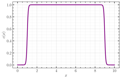
Figure 1: Smooth boxcar function used for the hyper-viscosity operator.

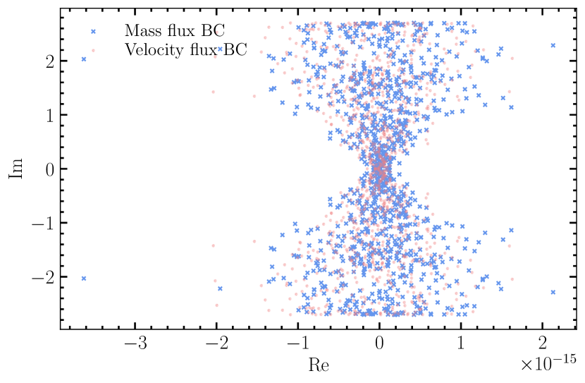
(a) $\alpha=0$

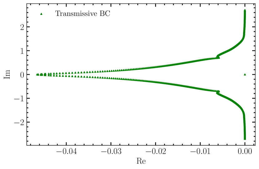
(b) $\alpha=0$

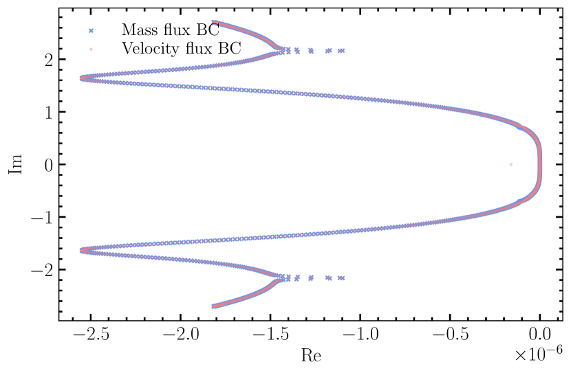
(c) $\alpha=0.1\Delta{x}^{3}$

(d) $\alpha=0.1\Delta{x}^{3}$

Figure 2: Numerical eigenspectra of the DP operators of order 6 with $N=501$, $g=H=1$, for the three main BCs considered using SAT terms: mass flux, velocity flux and transmissive BCs. The first two are energy conserving without hyperviscosity and maintains zero real parts up to machine error, while adding hyperviscosity and utilising transmissive BCs should dissipate energy, which yields non-positive real parts. All spectra clearly indicate strict stability of the eigensystem.

In the next section we present numerical experiments in 1D verifying the theory derived in this paper. We will also present some 2D numerical simulations showing extensions of the method 2D nonlinear rotating shallow water equations.

7 Numerical experiments

In this section we present detailed numerical experiments verifying the theoretical analysis performed in the previous sections. In particular the experiments are designed to verify stability, accuracy and convergence properties of the method, including verification of the nonlinear transmissive boundary conditions. We also present canonical test problems such as the dam break with wet domain, and the well-balanced test called the lake at rest with non-smooth and smooth immersed bump. A numerical example in 2D within a doubly periodic domain is presented showing extension of the method to 2D and effectiveness of the hyper-viscosity operator for simulating merging vortexes.

For time discretisation, we use the classical fourth order accurate explicit Runge-Kutta method. Throughout the 1D numerical experiments, we set the global time step

$$\Delta t=\frac{\textrm{CFL}\times\Delta x}{\max_{x}{(|U|+\sqrt{gH})}},$$ (51)

where $\Delta x=L/N$, $N+1$ is the number of grid points and $\textrm{CFL}=0.3$. We use natural units, so that $g=9.81$, $H=1$, $U=-0.3\sqrt{gH}$, $|U|+\sqrt{gH}$ is the characteristic wave speed of the linear problems, and for the nonlinear problem we use $U=u(t=0,x)$ and $H=h(t=0,x)$.

7.1 Numerical experiments in 1D

We first study the accuracy of the numerical method via the method of manufactured solutions (MMS), before moving to canonical test problems such as the dam break problem with wet domain, and the well-balanced test called the lake at rest with non-smooth and smooth immersed bump, as proposed in [44].

7.1.1 Method of manufactured solutions

DP, order 4, MMS
Linear					nonlinear
$N$	$\log_{2}\|\textrm{error}\|_{2,u}$	$\log_{2}\|\textrm{error}\|_{2,h}$	$q_{u}$	$q_{h}$	$\log_{2}\|\textrm{error}\|_{2,u}$	$\log_{2}\|\textrm{error}\|_{2,h}$	$q_{u}$	$q_{h}$
(1)	(2)	(3)	(4)	(5)	(6)	(7)	(8)	(9)
41	-6.5665	-6.5454	-	-	-5.5362	-5.7156	-	-
81	-10.8428	-10.8198	4.2763	4.2743	-8.9666	-9.0302	3.4305	3.3146
161	-14.8953	-14.8755	4.0525	4.0557	-12.8307	-13.0011	3.9284	4.0598
321	-18.9189	-18.9011	4.0236	4.0256	-16.7592	-17.0609	3.9284	4.0598
641	-22.9305	-22.9139	4.0116	4.0127	-20.7279	-21.0780	3.9687	4.0171

DRP, order 4, MMS
Linear					nonlinear
$N$	$\log_{2}\|\textrm{error}\|_{2,u}$	$\log_{2}\|\textrm{error}\|_{2,h}$	$q_{u}$	$q_{h}$	$\log_{2}\|\textrm{error}\|_{2,u}$	$\log_{2}\|\textrm{error}\|_{2,h}$	$q_{u}$	$q_{h}$
(1)	(2)	(3)	(4)	(5)	(6)	(7)	(8)	(9)
41	-4.2724	-4.7107	-	-	-4.2123	-4.3524	-	-
81	-10.7031	-10.7447	6.4307	6.0341	-9.3048	-8.5032	5.0925	4.1508
161	-10.7031	-10.7447	4.4595	4.3913	-12.9814	-12.8435	3.6765	4.3403
321	-15.1626	-15.1360	4.4595	4.3913	-16.8969	-17.1903	3.9155	4.3468
641	-23.1426	-23.1243	3.9983	4.0011	-20.8564	-21.2958	3.9596	4.1054

DP, order 6, MMS
Linear					nonlinear
$N$	$\log_{2}\|\textrm{error}\|_{2,u}$	$\log_{2}\|\textrm{error}\|_{2,h}$	$q_{u}$	$q_{h}$	$\log_{2}\|\textrm{error}\|_{2,u}$	$\log_{2}\|\textrm{error}\|_{2,h}$	$q_{u}$	$q_{h}$
(1)	(2)	(3)	(4)	(5)	(6)	(7)	(8)	(9)
41	-5.9761	-5.0590	-	-	-5.6406	-4.7045	-	-
81	-10.5185	-10.4705	4.5424	5.4115	-10.2011	-10.5153	4.5605	5.8108
161	-15.5532	-15.2167	5.0348	4.7461	-15.1654	-14.7981	4.9643	4.2828
321	-20.1258	-19.7233	4.5726	4.5067	-19.7564	-19.2424	4.5910	4.4443
641	-24.7807	-24.2329	4.6549	4.5095	-24.4788	-23.7511	4.7224	4.5087

DRP, order 6, MMS
Linear					nonlinear
$N$	$\log_{2}\|\textrm{error}\|_{2,u}$	$\log_{2}\|\textrm{error}\|_{2,h}$	$q_{u}$	$q_{h}$	$\log_{2}\|\textrm{error}\|_{2,u}$	$\log_{2}\|\textrm{error}\|_{2,h}$	$q_{u}$	$q_{h}$
(1)	(2)	(3)	(4)	(5)	(6)	(7)	(8)	(9)
41	-3.9230	-5.2152	-	-	-3.1407	-4.1012	-	-
81	-8.3058	-9.0906	4.3827	3.8754	-8.0456	-8.6623	4.9049	4.5611
161	-14.3327	-14.1198	6.0270	5.0292	-13.7421	-13.7835	5.6965	5.1212
321	-18.9399	-18.3042	4.6072	4.1844	-18.3152	-17.6874	4.5731	3.9039
641	-23.4452	-22.7525	4.5053	4.4483	-22.8357	-22.1028	4.5205	4.4154

Table 1: log 2 $L^{2}$ norm errors and convergence rate of various finite difference operators using MMS, for the primitive variables $u$,$h$.

In this section, we use MMS to verify the convergence of our numerical scheme. We consider both linear and nonlinear problems. The computational domain is $x\in[0,L]$ with length $L=10$. We force the system with the exact solution

$$u_{e}(x,t)=\exp(-(x-x_{0}-c_{s}t)^{2}),\quad h_{e}(x,t)=u_{e}(x,t)+10,\quad x_{0}=0.5L,\quad c_{s}=\sqrt{gH},$$ (52)

while enforcing the linear mass flux BC $F_{1}(x,t):=Hu(x,t)+Uh(x,t)=Hu_{e}(x,t)+Uh_{e}(x,t)$ at $x=0,L$ for the linear problem and the nonlinear mass flux BC $F_{1}(x,t):=u(x,t)h(x,t)=u_{e}(x,t)h_{e}(x,t)$ at $x=0,L$ for the nonlinear problem. Note that $Hu_{e}(x,t)+Uh_{e}(x,t)$ and $u_{e}(x,t)h_{e}(x,t)$ yield nonzero boundary data. We run the simulations until the final time $t=0.5$.

MMS without hyper-viscosity.

We consider first grid convergence tests without hyper-viscosity and proceed later to convergence tests with hyper-viscosity. The numerical errors and convergence rates for different operators, without hyper-viscosity, for the linear and nonlinear cases are reported in Table 1. As has already been noted in prior works [36, 45, 16], the diagonal norm DP upwind operators have “higher than expected” convergence rates. Our experiments also show that the DRP operators exhibit the same behaviour, higher than expected convergence rates, as it also satisfy the upwind property. We do not understand the precise reason for this yet, further analysis is needed to unravel the super-convergence properties exhibited by the schemes. For additional convergence studies using traditional SBP operators, and odd-order upwind DP and DRP operators, see Appendix A

MMS with hyper-viscosity.

We now assess the accuracy of the method with hyper-viscosity for linear and nonlinear problems. To do this we use MMS and perform grid convergence studies for smooth solutions. We set $\alpha=\delta{\Delta{x}}^{p-1}$ and $\delta=0.1$, where $p=4,6$ for $4$th and $6$th order derivative hyper-viscosity operators. For smooth solutions the truncation error for the hyper-viscosity operators is $\mathbb{T}\sim{\Delta{x}}^{p-1}+\mathcal{O}({\Delta x}^{p})$. We expect the convergence rate of the errors to be at most $\mathcal{O}({\Delta x}^{p-1})$. Table 2 shows the error and convergence rates of the error for DP upwind and DRP operators of $4$ and $6$ interior accuracy, for linear and nonlinear problems. Hence, our DP and DRP schemes remain high order accurate with hyper-viscosity for smooth solutions, for both linear and nonlinear problems.

DP order 4, hyper-viscosity, MMS
Linear					nonlinear
$N$	$\log_{2}\|\textrm{error}\|_{2,u}$	$\log_{2}\|\textrm{error}\|_{2,h}$	$q_{u}$	$q_{h}$	$\log_{2}\|\textrm{error}\|_{2,u}$	$\log_{2}\|\textrm{error}\|_{2,h}$	$q_{u}$	$q_{h}$
(1)	(2)	(3)	(4)	(5)	(6)	(7)	(8)	(9)
41	-7.1027	-6.2709	0	0	-6.7094	-5.9420	0	0
81	-11.3750	-11.0446	4.2723	4.7738	-11.1816	-10.8197	4.4722	4.8777
161	-15.8828	-15.6486	4.5078	4.6040	-15.4499	-15.0417	4.2683	4.2220
321	-19.4923	-19.4737	3.6095	3.8251	-18.8463	-18.3501	3.3964	3.3084

DRP order 4, hyper-viscosity, MMS
Linear					nonlinear
$N$	$\log_{2}\|\textrm{error}\|_{2,u}$	$\log_{2}\|\textrm{error}\|_{2,h}$	$q_{u}$	$q_{h}$	$\log_{2}\|\textrm{error}\|_{2,u}$	$\log_{2}\|\textrm{error}\|_{2,h}$	$q_{u}$	$q_{h}$
(1)	(2)	(3)	(4)	(5)	(6)	(7)	(8)	(9)
41	-7.1027	-6.2709	0	0	-3.8329	-4.01740	0	0
81	-11.3750	-11.0446	4.2723	4.7738	-8.7963	-10.9147	4.9633	6.8973
161	-15.8828	-15.6486	4.5078	4.6040	-14.2213	-14.0322	5.4250	3.1175
321	-19.4923	-19.4737	3.6095	3.8251	-18.5059	-17.9750	4.2846	3.9429

DP order 6, hyper-viscosity, MMS
Linear					nonlinear
$N$	$\log_{2}\|\textrm{error}\|_{2,u}$	$\log_{2}\|\textrm{error}\|_{2,h}$	$q_{u}$	$q_{h}$	$\log_{2}\|\textrm{error}\|_{2,u}$	$\log_{2}\|\textrm{error}\|_{2,h}$	$q_{u}$	$q_{h}$
(1)	(2)	(3)	(4)	(5)	(6)	(7)	(8)	(9)
41	-7.0942	-6.2723	0	0	-6.6884	-5.9477	0	0
81	-11.4008	-11.0658	4.2723	4.7738	-11.2279	-10.8404	4.5396	4.8927
161	-16.2131	-15.8455	4.5078	4.6040	-15.9767	-15.4594	4.7487	4.6190
321	-20.9717	-20.5254	4.7586	4.6798	-20.6898	-20.1138	4.7131	4.6544

DRP order 6, hyper-viscosity, MMS
Linear					nonlinear
$N$	$\log_{2}\|\textrm{error}\|_{2,u}$	$\log_{2}\|\textrm{error}\|_{2,h}$	$q_{u}$	$q_{h}$	$\log_{2}\|\textrm{error}\|_{2,u}$	$\log_{2}\|\textrm{error}\|_{2,h}$	$q_{u}$	$q_{h}$
(1)	(2)	(3)	(4)	(5)	(6)	(7)	(8)	(9)
41	-4.2029	-4.7415	0	0	-3.8306	-4.0142	0	0
81	-9.2636	-10.1468	5.0607	5.4053	-8.7986	-11.1187	4.4.968	7.1045
161	-14.9135	-14.6628	3.8338	3.9573	-14.3236	-14.0398	5.5251	2.9211
321	-19.7461	-19.0091	4.8326	4.3463	-19.1884	-18.4021	4.8648	4.3623

Table 2: log 2 $L^{2}$ norm errors and convergence rate of the DP and DRP operators of order $p=4,6$ interior operators, with hyper-viscosity pre-factor $\delta=0.1$.

7.1.2 Lake at rest with immersed bump

We consider the canonical 1D lake at rest problem, modeled by the nonlinear SWE (2) with bottom topography (immersed bump), as described in [44]. The length of the domain is $L=25$ and the bottom topography embedded below the fluid is modelled as:

$$b(x)=\begin{cases}0.2-0.05(x-10)^{2}&\text{ if }8<x<12,\\ 0&\text{ $x\in\Omega\backslash\{8,12\}$},\end{cases}$$ (53)

The bottom topography $b(x)$ enters the nonlinear SWE (2) through its derivative

$${b^{\prime}(x)}=\begin{cases}-0.1(x-10)&\text{ if }8<x<12,\\ 0&\text{ $x\in\Omega\backslash\{8,12\}$},\end{cases}$$ (54)

which appears as a source term in the momentum equation. Note that $b^{\prime}(x)$ is discontinuous at $x=\{8,12\}$.

No perturbation.

We will now verify the well-balanced property of the numerical method. We prescribe the initial condition

$$h(x,0)+b=0.5,\quad u(x,0)=0,$$

throughout the domain. As the initial conditions solve a steady state problem, a good numerical scheme should maintain the prescribed initial condition for all time. Following [16], we prescribe periodic BCs at $x=0,L$, with periodic finite difference stencils. No hyper-viscosity is used for this test case, despite the fact that $b(x)$ is non-smooth. As shown in Fig. 3, our scheme maintains both heights and velocities at the analytical value up to machine error. This is independent of the grid resolution, and confirms the well-balanced property of the numerical scheme.

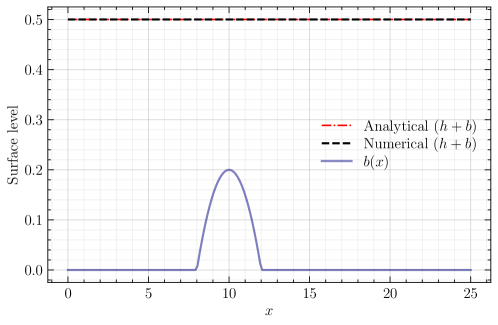
Figure 3: Plot of the height for the canonical lake at rest problem at end time $t=5$, where the topography $b(x)$ is defined via (53), which is non-smooth about $x\in(8,12)$. The simulation is initialised with $h+b=0.5$, $N=201$, $L=25$. Our numerical scheme maintains the initial condition up to machine precision.

FD, order 6, Lake at Rest
	$\log_{10}\|\textrm{error}\|_{2,u}$	$\log_{10}\|\textrm{error}\|_{2,u}$	$\log_{10}\|\textrm{error}\|_{2,u}$
$N$	(SBP)	(DP)	(DRP)
51	-14.6270	-14.0611	-15.4622
101	-14.3264	-13.7623	-15.1600
151	-14.1503	-13.5869	-14.9836
201	-14.0253	-12.7646	-14.8581

Table 3: Log10 error of the lake at rest’s velocity profile, it can be seen that all operators achieve values near machine precision, regardless of grid resolution.

Small perturbations.

The aim of this experiment is to verify the implementation and accuracy of the nonlinear transmissive boundary conditions (21). As above we consider the 1D lake at rest problem, with zero initial condition for velocity, $u(x,0)=0$, and we add small perturbations to the initial condition for height,

$$h(x,0)=0.5-b(x)+\delta{b}(x),\quad\delta{b}(x)=0.1\max_{x}{|b(x)|}\times e^{-\frac{\left(x-10\right)^{2}}{0.3}}.$$

The perturbation will generate variations in both height and velocity which will propagate through the domain. However, the variations introduced by the perturbation are expected to leave the domain through the transmissive boundaries without reflections.

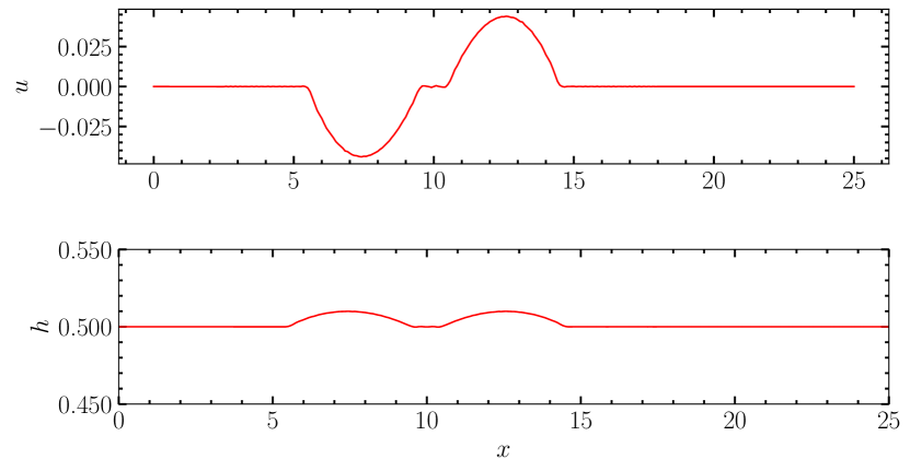
(a) $t=100\Delta t$

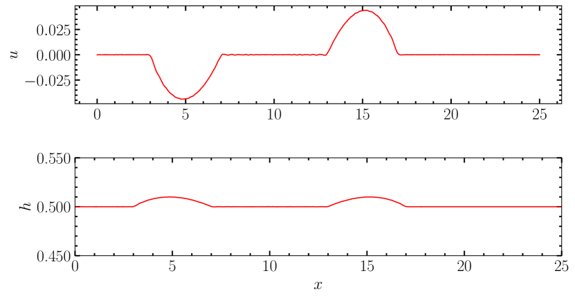
(b) $t=200\Delta t$

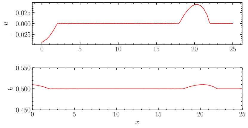
(c) $t=400\Delta t$

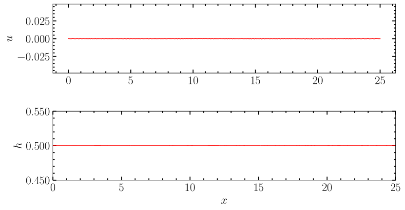
(d) $t=800\Delta t$

Figure 4: Time evolution of the lake at rest profile with 10% perturbations on $h$ with transmissive BC. The waves transmit out the right and left boundaries to maintain an overall steady state flowfield similar to the caonical lake at rest problem.

FD, order 6, Lake at Rest, smooth perturbations
$N$	(SBP)		(DP)		(DRP)
	$q_{u}$	$q_{h}$	$q_{u}$	$q_{h}$	$q_{u}$	$q_{h}$
101	-	-	-	-	-
201	2.0126	1.8438	2.6958	2.8914	2.2873	1.6657
401	2.9720	2.9958	3.6705	3.5118	2.7088	2.8301
801	3.9608	3.8156	5.5908	5.5869	3.9935	4.1396

Table 4: Convergence rate of the lake at rest problem with small perturbations on $h$ ($10\%$), with smooth topography of the Gaussian form, see (7.1.2). Satisfactory convergence rates are achieved with smooth $b(x)$.

In Fig. 4 we show the time evolution of the perturbed velocity and height profiles. Clearly the perturbations leave the domain without reflections, and we recover the steady state solutions. We have also performed grid convergence studies, see Table 4 for the convergence rates of the numerical error. The errors converge to zero at an optimal rate for order 6 FD operators.

7.1.3 Dam break with wet domain

Next, we investigate the efficacy of the method in the presence of nonlinear shocks. We consider the canonical dam break problem [44] in a wet domain with the following initial conditions:

$$h(x,t=0)=\begin{cases}h_{l}&\text{ if }0\leq x\leq x_{0},\\ h_{r}&\text{ if }x_{0}<x\leq L,\end{cases}\qquad u(x,t=0)=0,$$ (55)

where we use $x_{0}=5$, $h_{l}=1$, $h_{r}=0.5$ and $L=10$. Note that the initial condition for the water height is discontinuous at $x=x_{0}$. The exact solutions consists of a right-going shock front and a left-going rarefaction fan. Using the method of characteristics the exact solution has the closed form expression [44]

$$h(t,x)=\left\{\begin{array}[]{l}h_{l}\\ \frac{4}{9g}\left(\sqrt{gh_{l}}-\frac{x-x_{0}}{2t}\right)^{2}\\ \frac{c_{m}^{2}}{g}\\ h_{r}\end{array}\right.,\;u(t,x)=\begin{cases}0&\text{ if }x\leq x_{A}(t),\\ \frac{2}{3}\left(\frac{x-x_{0}}{t}+\sqrt{gh_{l}}\right)&\text{ if }x_{A}(t)\leq x\leq x_{B}(t),\\ 2\left(\sqrt{gh_{l}}-c_{m}\right)&\text{ if }x_{B}(t)\leq x\leq x_{C}(t),\\ 0&\text{ if }x_{C}(t)\leq x,\end{cases}$$

where subscripts $l$ and $r$ denote left and right, and $x_{A}$, $x_{B}$, $x_{C}$ satisfy the following evolution equations, with $c_{m}$ defined as a solution to the algebraic equation,

$$-8gh_{r}c_{m}^{2}\left(\sqrt{gh_{l}}-c_{m}\right)^{2}+\left(c_{m}{}^{2}-gh_{r}\right)^{2}\left(c_{m}{}^{2}+gh_{r}\right)=0$$

and the coordinates, $x_{A},x_{B},x_{C}$ are defined by

$$x_{A}(t)=x_{0}-t\sqrt{gh_{l}},\quad x_{B}(t)=x_{0}+t\left(2\sqrt{gh_{l}}-3c_{m}\right)\text{ and }x_{C}(t)=x_{0}+t\frac{2c_{m}^{2}\left(\sqrt{gh_{l}}-c_{m}\right)}{c_{m}^{2}-gh_{r}}.$$ (56)

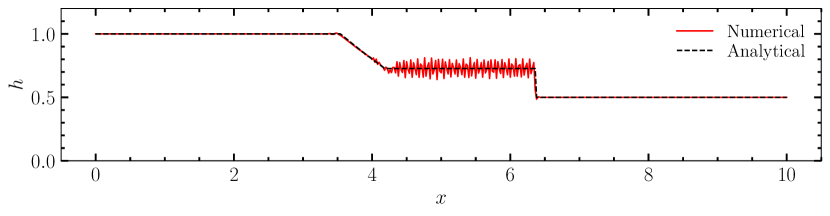
(a) Without hyperviscosity

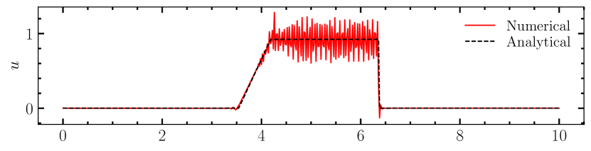
(b) Without hyperviscosity

(c) With hyperviscosity, $\delta=0.1$

(d) With hyperviscosity, $\delta=0.1$

Figure 5: Time evolution of the height and velocity profile of the dam break with wet domain problem, with the overlaid analytical solution using the DP order 6 operators, $N=501$, showing time snapshot at $t=1000\Delta t$, comparing the solutions with and without hyperviscosity. Clearly the oscillations are heavily amplified in those without.

To perform numerical simulations we close the boundaries with transmissive boundary conditions and discretise the computational domain with $N=1001$ grid points. We run the simulation until the final time $t=2$ using the $6$th order accurate DP SBP operators, with hyper-viscosity $\delta=0.1$ and without hyper-viscosity $\delta=0$. In Figure 5 we compare numerical solutions with the exact solutions at $t=1000\Delta{t}$. Note that the numerical solution is stable and the shock speed and the rarefaction fan are well resolved by our high order numerical method. However, without hyper-viscosity there are spurious oscillations from the shock front which pollute the numerical solutions. The addition of the hyper-viscosity, with $\delta=0.1$, eliminates the oscillations without destroying the high order accuracy of the solution in smooth regions. Furthermore, in Figs. 6 and 7 we show the time evolution of the height and velocity, with hyper-viscosity. It is clearly demonstrated that the numerical and analytical solutions agree well, despite the presence of shocks and the highly nonlinear nature of the flow problem.

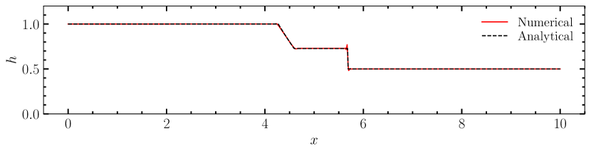
(a) $t=1000\Delta t$

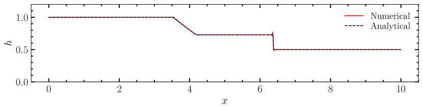
(b) $t=2000\Delta t$

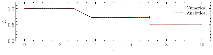
(c) $t=3000\Delta t$

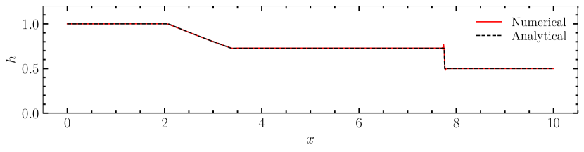
(d) $t=4000\Delta t$

Figure 6: Time evolution of the height profile of the dam break with wet domain problem, with the overlaid analytical solution using the DRP order 6 operators, $N=1001$, with final time $t=1$. The hyperviscosity parameter is set to $\delta=0.1$

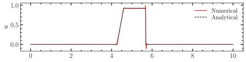
(a) $t=1000\Delta t$

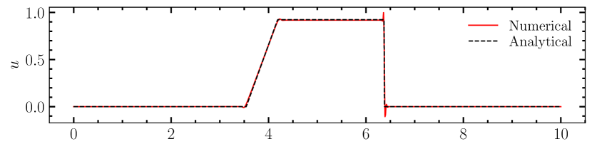
(b) $t=2000\Delta t$

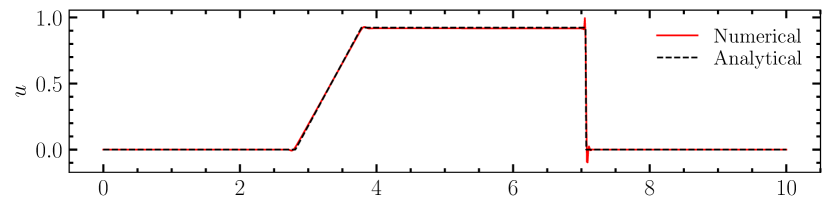
(c) $t=3000\Delta t$

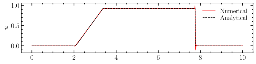
(d) $t=4000\Delta t$

Figure 7: Same as Fig. 6 but for the time evolution of the velocity profile.

7.2 2D merging vortex problem

As an extension to the 1D numerical experiments to 2D, we consider the “merging vortex problem” [46]. This problem is modelled by the 2D rotating shallow water equations (1) in the spatial domain $\Omega=(0,2\pi]\times(0,2\pi]$ with periodic boundary conditions. The the initial conditions are a pair of Gaussian vortex with the in-compressible stream function

$$\psi=e^{-5\left((y-\pi)^{2}+(x-2.6\pi/3)^{2}\right)}+e^{-5\left((y-\pi)^{2}+(x-3.5\pi/3)^{2}\right)}.$$ (57)

The initial conditions for the velocity field are defined through $\mathbf{u}(x,y,0)=\nabla^{\perp}\psi$, $\nabla^{\perp}=(-\partial_{y},\partial_{x})$ and the initial condition for water height $h$ is obtained from linear geostrophic balance $f\times\mathbf{u}^{\perp}(x,y,0)+g\times\nabla h(x,y,0)=0\implies h(x,y,0)=H+f/g\times\psi(x,y)$, with $f=g=H=8$.

The continuous 2D rotating shallow water equations (1) preserves infinitely many invariants. However, any discrete approximation can (approximately) preserve a finite number of invariants [22]. For the numerical approximation we select a subset of the invariants, namely: 1) total energy/entropy $E(t)$, 2) total enstrophy $E_{s}(t)$, 3) total vorticity $W(t)$ and 4) total mass $M(t)$, defined by

$$E(t)=\int_{\Omega}edxdy,\quad{E}_{\mathrm{s}}(t)=\int_{\Omega}\omega^{2}hdxdy,\quad{W}(t)=\int_{\Omega}\omega dxdy,\quad M(t)=\int_{\Omega}hdxdy,$$ (58)

which the numerical method should accurately preserve. Here, $e=\frac{1}{2}\left(gh^{2}+hu^{2}+hv^{2}\right)$ is the elemental energy/entropy and $\omega$ is the absolute vorticity defined in (1). The energy/entropy $E(t)$ is critical for nonlinear stability. The enstrophy ${E}_{\mathrm{s}}$ is a higher order moment and bounds the derivatives of the solution. More importantly the enstrophy is crtical for controlling grid-scale errors and ensuring that high frequency oscillations do not ruin the accuracy of the solution.

The numerical approximations of the invariants are given by

$$\mathcal{E}(t)=\sum^{N}_{ij}e_{ij}\Delta x\Delta y,\quad\mathcal{E}_{\mathrm{s}}(t)=\sum^{N}_{ij}\omega^{2}_{ij}h_{ij}\Delta x\Delta y,\quad\mathcal{W}(t)=\sum^{N}_{ij}\omega_{ij}\Delta x\Delta y,\quad\mathcal{M}(t)=\sum^{N}_{ij}h_{ij}\Delta x\Delta y,$$ (59)

where $e_{ij}$ and $\boldsymbol{\omega}$ are defined in (61) and (63), respectively, and where $i,j$ are indices corresponding to grid points. We define the relative changes in the discrete invariants

$$\Delta_{r}{\mathcal{E}}(t)=\frac{\mathcal{E}(t)-\mathcal{E}(0)}{\mathcal{E}(0)},\quad\Delta_{r}{\mathcal{E}}_{s}(t)=\frac{\mathcal{E}_{s}(t)-\mathcal{E}_{s}(0)}{\mathcal{E}_{s}(0)},\quad\Delta_{r}{\mathcal{W}}(t)=\frac{\mathcal{W}(t)-\mathcal{W}(0)}{\mathcal{W}(0)},\quad\Delta_{r}{\mathcal{M}}(t)=\frac{\mathcal{M}(t)-\mathcal{M}(0)}{\mathcal{M}(0)}.$$ (60)

The semi-discrete approximation of the 2D rotating shallow water equations (1) using the dual-pairing SBP framework is derived in Appendix B. In Theorem 13, we prove that the semi-discrete approximation conserves the discrete energy/entropy without hyper-viscosity $\delta=0$ and dissipates energy/entropy with hyper-viscosity $\delta>0$. Semi-discrete conservation of total mass and vorticity also follow, but the proofs are not given.

As before, the semi-discrete approximations are evolved in time using classical fourth order accurate explicit Runge-Kutta method with $\operatorname{CFL}=0.1$. In Fig. 9 we show snapshots of potential vorticity using DP SBP operators of order 4 on a uniform grid of size $251^{2}$ grid points. The left panel shows the snapshots of the numerical solution without hyper-viscosity ($\delta=0$) and right panel shows the snapshots of the numerical solution with hyper-viscosity ($\delta=0.5$). It is significantly noteworthy that in both cases the numerical solutions remain bounded through out the simulation. This is consistent with the energy stability proof of Theorem 13. However, without hyper-viscosity ($\delta=0$, left panel), the structure in the solution is completely destroyed by spurious numerical artefacts. The addition of hyper-viscosity to the scheme ($\delta=0.5$, right panel) eliminates the spurious wave modes which can destroy the accuracy of the numerical solution. With hyper-viscosity the numerical method preserves approximate geostrophic balance and the solution remains accurate throughout the simulation. The numerical solutions are comparable to the results given in the literature [46] using compatible finite element methods. We also note that in [46], in order to tame poisonous numerical oscillations the authors utilised the so-called Artificial Potential Vorticity Method (APVM) for the finite element method. In general for nonlinear problems, energy/entropy conservation although ensures the boundedness of numerical solutions but it does not guarantee convergence of numerical errors. Suitable amount of numerical dissipation is necessary to control high frequency errors.

We also compute the relative change in the discrete invariants (59) as defined in (60). The time evolution of relative change in the discrete invariants are shown Figs. 10 and 11 for DP and DRP SBP operators of order 4 and 6. Note that total mass, energy and vorticity are conserved up to the grid resolution. Without hyper-viscosity the enstrophy grows linearly leading to the growth of high frequency errors which pollutes the solutions. With the addition hyper-viscosity the magnitude of the enstrophy is relatively smaller and decay linearly with time.

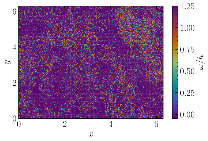
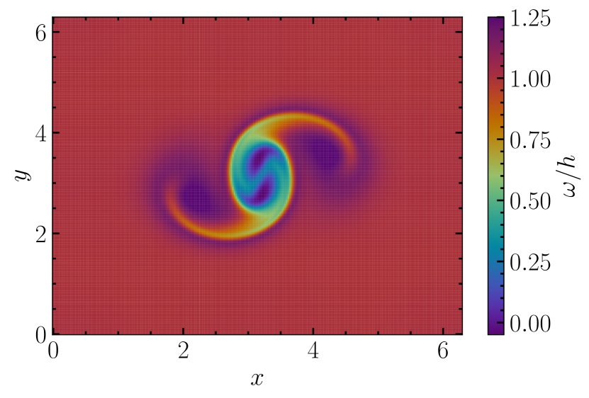
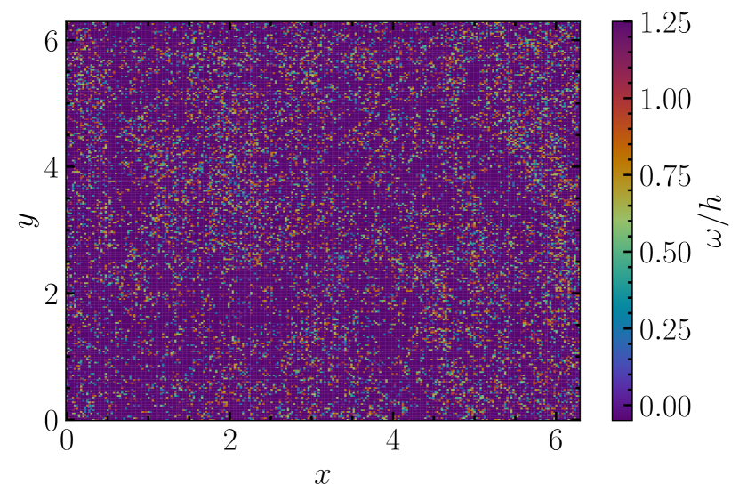
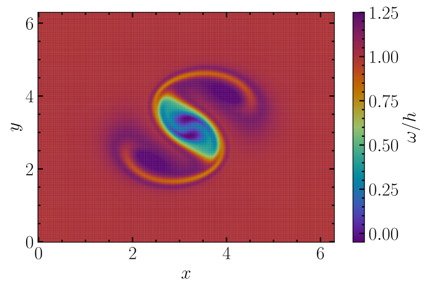
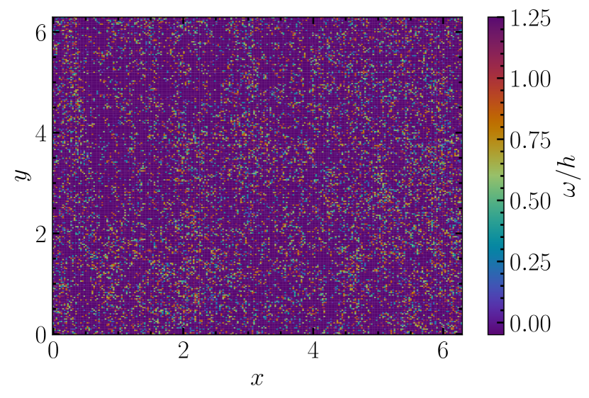
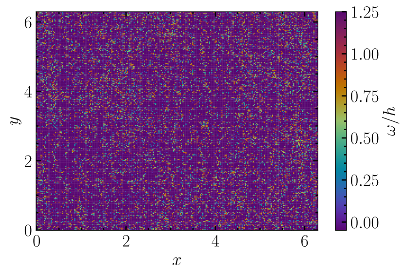
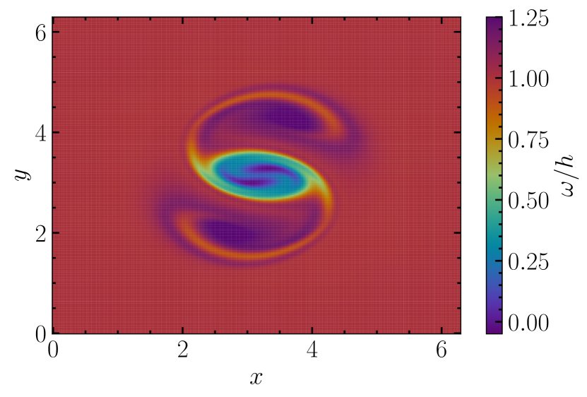
Figure 9: Potential vorticity, $\omega/h$ for the 2D merging vortex problem (57) using DP operators of order 4. The left panels show the solutions without hyperviscosity, while the right show those with hyperviscosity, where $\delta=0.5$. Snapshots are at $t=0,0.3,0.7,1.5,2.0,3.0,3.5,3.9$.

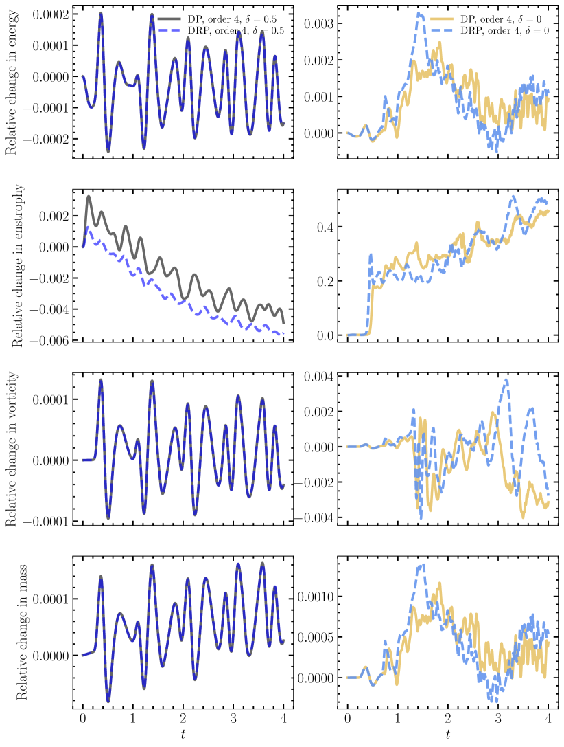
Figure 10: Relative change of the total energy, vorticity, enstrophy and mass for the 2D merging vortex problem using DP operators of order 4. Clearly, energy and vorticity remains conserved up to grid resolution, but enstrophy is dissipated due to the introduction of hyperviscosity.

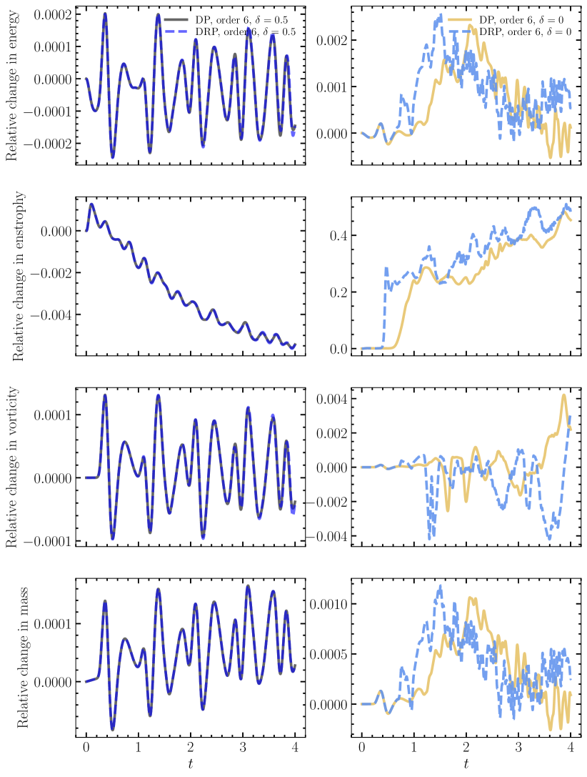
Figure 11: Same as Fig. 10 but for order 6 DP and DRP operators.

8 Conclusion

A novel, energy/entropy stable, and high order accurate numerical scheme has been developed and analysed to solve the 1D and 2D nonlinear shallow water equations in vector invariant form. The scheme is suitable for the simulations of sub-critical flow regimes typical prevalent in atmospheric and geostrophic flow problems. The numerical scheme is based on the recently derived high order accurate dual-pairing SBP operators [36, 37, 47]. The method has been validated with a number of canonical test cases as well as with the method of manufactured smooth solutions, including 2D merging vortex problems.

For nonlinear problems, energy/entropy stability although ensures the boundedness of numerical solutions but it does not guarantee convergence of numerical errors with mesh refinement. Suitable amount of numerical dissipation is necessary to control high frequency errors which could ruin numerical simulations. Using the dual-pairing SBP framework, we designed high order accurate and nolinear hyper-viscosity operator which dissipates entropy. The hyper-viscosity operator effectively tames oscillations from shocks and discontinuities and eliminates poisonous high frequency grid-scale errors.

Another important results here are new well-posed boundary conditions for the 1D vector invariant form of the SWEs formulated in terms of fluxes of the primitive variables, and applicable to linear and nonlinear problems. We prove that the boundary conditions are well-posed and energy/entropy stable. Numerical experiments are performed to verify the theoretical results, and in particular the nonlinear transmissive boundary conditions.

Future work will extend the method to spherical and complex geometries using curvilinear grids. We will also extend the 1D nonlinear boundary conditions to 2D which will enable efficient numerical simulations in non-periodic bounded domains.

9 Acknowledgements

We thank Kenny Wiratama, Kieran Ricardo and David Lee for insightful discussions about higher order discretisation methods for hyperbolic systems. We are also grateful to Christopher Williams, Alberto Martín, Rudi Prihandoko, James R. Beattie and Neco Kriel for general discussions regarding this work. J. K. J. H. acknowledges funding via the ANU Chancellor’s International Scholarship, the Space Plasma, Astronomy and Astrophysics Research Award, the Boswell Technologies Endowment Fund and Higher Degree Research (HDR) Award for Space Exploration. We also acknowledge computational resources provided by the National Computational Infrastructure (NCI) under the grant xx52, which is supported by the Australian Government.

10 Data Availability Statement

The datasets produced/analysed in the present study are available upon reasonable request to the corresponding author (J.K.J.H.).

Appendix A Additional convergence studies for traditional SBP and odd-order DP and DRP operators

Here in Tables 5 and 6, we show additional convergence tables with the Gaussian MMS conducted using the traditional SBP operators (Table 5), as well as odd-order DP and DRP operators (Table 6). As confirmed earlier, we observe superconvergence for 4th and 6th order SBP operators. However, traditional SBP operators achieve globally $3$rd order convergence rate for order 4 interior operator, consistent with the $p+1$ global accuracy expected from Laplace transform analysis, and $5$th order global convergence rate for order 6 interior operator.

However, as shown in Table 6, the DP and DRP odd order operators exhibit super-convergent behaviour, which has also been shown in a number of recent works [36, 45, 16], due to the nature of these types of upwind SBP operators, while we note that the precise reason for this is still unknown.

SBP, order 4, MMS
Linear					nonlinear
$N$	$\log_{2}\|\textrm{error}\|_{2,u}$	$\log_{2}\|\textrm{error}\|_{2,h}$	$q_{u}$	$q_{h}$	$\log_{2}\|\textrm{error}\|_{2,u}$	$\log_{2}\|\textrm{error}\|_{2,h}$	$q_{u}$	$q_{h}$
(1)	(2)	(3)	(4)	(5)	(6)	(7)	(8)	(9)
41	-5.8130	-5.7980	-	-	-8.7047	-8.6876	-	-
81	-8.9000	-8.8860	3.0870	3.0880	-5.0059	-5.1572	3.6988	3.5304
161	-11.9541	-11.9402	3.0541	3.0542	-11.9884	-11.9613	3.2837	3.2737
321	-14.9679	-14.9541	3.0139	3.0139	-15.0822	-15.0326	3.0937	3.0714
641	-17.9714	-17.9576	3.0035	3.0035	-18.1097	-18.0501	3.0276	3.0175

SBP, order 6, MMS
Linear					nonlinear
$N$	$\log_{2}\|\textrm{error}\|_{2,u}$	$\log_{2}\|\textrm{error}\|_{2,h}$	$q_{u}$	$q_{h}$	$\log_{2}\|\textrm{error}\|_{2,u}$	$\log_{2}\|\textrm{error}\|_{2,h}$	$q_{u}$	$q_{h}$
(1)	(2)	(3)	(4)	(5)	(6)	(7)	(8)	(9)
41	-5.5447	-5.4670	-	-	-4.1892	-4.1338	-	-
81	-9.5738	-9.5487	4.0291	4.0817	-9.1780	-9.1673	4.9888	5.0335
161	-15.1548	-15.1388	5.5810	5.5901	-14.7453	-14.7211	5.5673	5.5538
321	-20.3594	-20.3471	5.2047	5.2083	-19.8871	-19.8401	5.1417	5.1190
641	-25.3107	-25.3672	4.9513	5.0201	-24.8160	-24.8400	4.9289	4.9999

Table 5: log 2 $L^{2}$ norm errors and convergence rate of SBP operators of even order (order 4 and 6) for primitive variables $u,h$.

DP, order 5, MMS
Linear					nonlinear
$N$	$\log_{2}\|\textrm{error}\|_{2,u}$	$\log_{2}\|\textrm{error}\|_{2,h}$	$q_{u}$	$q_{h}$	$\log_{2}\|\textrm{error}\|_{2,u}$	$\log_{2}\|\textrm{error}\|_{2,h}$	$q_{u}$	$q_{h}$
(1)	(2)	(3)	(4)	(5)	(6)	(7)	(8)	(9)
41	-7.2370	-7.1095	-	-	-7.0995	-6.7450	-	-
81	-11.3378	-10.9423	4.1008	3.8328	-11.6030	-10.6515	4.5035	3.9064
161	-15.2832	-15.0097	3.9454	4.0674	-15.4952	-14.7624	3.8921	4.1109
321	-18.9627	-18.8146	3.6795	3.8049	-19.1202	-18.6201	3.6250	3.8577
641	-22.5701	-22.5139	3.6074	3.6993	-22.7087	-22.3616	3.5885	3.7415

DRP, order 5, MMS
Linear					nonlinear
$N$	$\log_{2}\|\textrm{error}\|_{2,u}$	$\log_{2}\|\textrm{error}\|_{2,h}$	$q_{u}$	$q_{h}$	$\log_{2}\|\textrm{error}\|_{2,u}$	$\log_{2}\|\textrm{error}\|_{2,h}$	$q_{u}$	$q_{h}$
(1)	(2)	(3)	(4)	(5)	(6)	(7)	(8)	(9)
41	-6.7009	-5.7814	-	-	-6.5358	-5.1352	-	-
81	-10.2166	-9.7475	3.5158	3.9661	-10.1635	-9.2776	3.6276	4.1424
161	-14.2013	-13.9006	3.9846	4.1531	-14.1764	-13.5178	4.0129	4.2402
321	-17.9694	-17.8282	3.7681	3.9276	-17.9550	-17.5155	3.7786	3.9977
641	-21.6402	-21.6193	3.6708	3.7911	-21.6441	-21.3592	3.6891	3.8437

Table 6: log 2 $L^{2}$ norm errors and convergence rate of DP and DRP operators of odd order (order 5) for primitive variables $u,h$.

Appendix B 2D energy/entropy stable semi-discrete approximation

To extend the 1D semi-discrete approximation (35) to the 2D rotating SWE (1) we discretise the 2D doubly-periodic domain $(x,y)\in\Omega=[0,2\pi]\times[0,2\pi]$ into $(N+1)\times(N+1)$ grid points $(x_{i},y_{j})=(i\Delta{x},j\Delta{y})$ with the uniform spatial step $\Delta{x}=\Delta{y}=2\pi/N$ for $N\in\mathbb{N}$. A 2D scalar field $v(x,y)$ on the grid $(x_{i},y_{j})$ is re-arranged row-wise into a vector $\mathbf{v}\in\mathbb{R}^{(N+1)^{2}}$. The 2D rotating SWE in semi-discrete form can be written as:

$$\frac{d\mathbf{h}}{dt}+\nabla_{\mathbf{D}_{+}}\cdot(\mathbf{U}\mathbf{h})=G_{h},\quad\frac{d\mathbf{U}}{dt}+\boldsymbol{\omega}\mathbf{U}^{\perp}+\nabla_{\mathbf{D}_{-}}\biggl{(}\frac{|\mathbf{U}|^{2}}{2}+g\mathbf{h}\biggl{)}=\mathbf{G}_{u}{\color[rgb]{0,0,1},}\quad\boldsymbol{\omega}=\mathbf{D}_{-x}\mathbf{v}-\mathbf{D}_{-y}\mathbf{u}+f_{c},\quad\mathbf{q}(0)=\mathbf{f},$$ (61)

where $\mathbf{U}=(\mathbf{u},\mathbf{v})^{T}$, $\mathbf{U}^{\perp}=(-\mathbf{v},\mathbf{u})^{T}$, $|\mathbf{U}|^{2}=\mathbf{u}^{2}+\mathbf{v}^{2}$, $\nabla_{\mathbf{D}_{\eta}}=(\mathbf{D}_{\eta x},\mathbf{D}_{\eta y})^{T}$, with $\eta\in\{+,-\}$. is the discrete approximation of gradient operator $\nabla=(\partial/\partial x,\partial/\partial y)^{T}$. As before, note that the derivatives for continuity equation are approximated with $D_{+}$ and the derivatives for the momentum equation are approximated with the dual operator $D_{-}$. Using the Kronecker product $\otimes$, the 2D DP derivative operators are defined as $\mathbf{D}_{\pm x}=D_{\pm}\otimes\mathbf{I}_{y}$, $\mathbf{D}_{\pm y}=\mathbf{I}_{x}\otimes D_{\pm}$ where $D_{\pm}$ are 1D DP operators closed with periodic boundary conditions, and satisfy $D_{+}+D_{-}^{T}=0$. The 2D SBP norm is defined as $\mathbf{P}=\Delta{x}\Delta{y}\mathbf{I}$ with $\mathbf{I}=\left(\mathbf{I}_{x}\otimes\mathbf{I}_{y}\right)$ and $\mathbf{I}_{x},\mathbf{I}_{y}\in\mathbb{R}^{(N+1)\times(N+1)}$ being identity matrices.

We define the 2D energy functional

$$\|\mathbf{q}\|_{\mathbf{P}\mathbf{W}^{\prime}}^{2}:=\mathbf{q}^{T}\left(\mathbf{P}\mathbf{W}^{\prime}\right)\mathbf{q}=\Delta{x}\Delta{y}\sum_{ij}\left(gh_{ij}^{2}+h_{ij}u_{ij}^{2}+h_{ij}v_{ij}^{2}\right),\quad\mathbf{W}^{\prime}=\begin{bmatrix}g\mathbf{I}&\mathbf{0}&\mathbf{0}\\ \mathbf{0}&\text{diag}(\mathbf{h})&\mathbf{0}\\ \mathbf{0}&\mathbf{0}&\text{diag}(\mathbf{h})\end{bmatrix},$$ (62)

and the elemental energy

$$e_{ij}:=\frac{1}{2}\left(gh_{ij}^{2}+h_{ij}u_{ij}^{2}+h_{ij}v_{ij}^{2}\right),$$ (63)

defines an entropy functional for sub-critical flows $u_{ij}^{2}+v_{ij}^{2}<gh_{ij}$. That is the elemental energy $e_{ij}$ is a convex function in terms of the prognostic variables $h_{ij},u_{ij},v_{ij}$. It is also noteworthy that

$$\mathbf{W}\mathbf{q}=\begin{bmatrix}\frac{|\mathbf{U}|^{2}}{2}+g\mathbf{h}\\ \mathbf{u}\mathbf{h}\\ \mathbf{v}\mathbf{h}\end{bmatrix},\ \mathbf{q}^{T}\left(\mathbf{P}\mathbf{W}\right)\frac{d\mathbf{q}}{dt}=\frac{1}{2}\frac{d}{dt}\biggl{(}\mathbf{q}^{T}\left(\mathbf{P}\mathbf{W}^{\prime}\right)\mathbf{q}\biggl{)},\ \mathbf{W}=\begin{bmatrix}g\mathbf{I}&\frac{1}{2}\text{diag}(\mathbf{u})&\frac{1}{2}\text{diag}(\mathbf{v})\\ \frac{1}{2}\text{diag}(\mathbf{u})&\frac{1}{2}\text{diag}(\mathbf{h})&0\\ \frac{1}{2}\text{diag}(\mathbf{v})&0&\frac{1}{2}\text{diag}(\mathbf{h})\end{bmatrix},\ \mathbf{W}=\mathbf{W}^{T}.$$ (64)

To make the 2D analysis amenable to the 1D theory we will reformulate the semi-discrete approximation (61). As before the 2D hyper-viscosity operator is constructed such that when appended to the semi-discrete formulation (61), it becomes,

$$\frac{d\mathbf{q}}{dt}+\nabla_{\mathbf{D}}\cdot\mathbf{F}+\mathbf{\Omega}_{f}=\mathbf{\mathcal{K}}\mathbf{q}+\mathbf{G},\quad\mathbf{\Omega}_{f}=\begin{bmatrix}\mathbf{0}\\ -\boldsymbol{\omega}\mathbf{v}\\ \boldsymbol{\omega}\mathbf{u}\end{bmatrix},\quad\boldsymbol{\omega}=\mathbf{D}_{-x}\mathbf{v}-\mathbf{D}_{-y}\mathbf{u}+f_{c},\quad\mathbf{q}(0)=\mathbf{f},$$ (65)

where $\nabla_{\mathbf{D}}\cdot\mathbf{F}=\mathbf{D}_{x}\mathbf{F}_{x}+\mathbf{D}_{y}\mathbf{F}_{y}$ and the flux and its gradients are given by

$$\mathbf{F}_{x}:=\begin{bmatrix}\mathbf{u}\mathbf{h}\\ \frac{|\mathbf{U}|^{2}}{2}+g\mathbf{h}\\ \mathbf{0}\end{bmatrix},\ \mathbf{F}_{y}:=\begin{bmatrix}\mathbf{v}\mathbf{h}\\ \mathbf{0}\\ \frac{|\mathbf{U}|^{2}}{2}+g\mathbf{h}\end{bmatrix},\quad\mathbf{D}_{x}\mathbf{F}_{x}:=\begin{bmatrix}\mathbf{D}_{+x}\left(\mathbf{u}\mathbf{h}\right)\\ \mathbf{D}_{-x}\left(\frac{|\mathbf{U}|^{2}}{2}+g\mathbf{h}\right)\\ \mathbf{0}\end{bmatrix},\ \mathbf{D}_{y}\mathbf{F}_{y}:=\begin{bmatrix}\mathbf{D}_{+y}\left(\mathbf{v}\mathbf{h}\right)\\ \mathbf{0}\\ \mathbf{D}_{-y}\left(\frac{|\mathbf{U}|^{2}}{2}+g\mathbf{h}\right)\end{bmatrix}.$$

Here the 2D nonlinear hyper-viscosity operator $\mathbf{\mathcal{K}}$ is given by

$$\mathbf{\mathcal{K}}=\mathbf{W}^{-1}\left(I_{3}\otimes\mathbf{P}^{-1}\right)\left(\left(I_{3}\otimes\mathcal{A}\otimes\mathbf{I}_{y}\right)+\left(I_{3}\otimes\mathbf{I}_{x}\otimes\mathcal{A}\right)\right),\quad\mathcal{A}=\mathcal{A}^{T},\quad\mathbf{u}^{T}\mathcal{A}\mathbf{u}\leq 0,\quad\forall\mathbf{u}\in\mathbb{R}^{N+1},$$ (66)

where $\mathcal{A}$ is the 1D hyper-viscosity operator derived in Section 6 and $I_{3}\in\mathbb{R}^{3\times 3}$ is the identity matrix.

We are now ready to prove that the numerical method (61) or (65) is strongly energy stable. Analogous to the 1D result Theorem 12 we also have

Theorem 13.

Consider the semi-discrete approximation (61) with periodic boundary conditions and the nonlinear hyper-viscosity operator $\mathcal{K}$ defined by (66). Let the symmetric matrix $\mathbf{W}$ and the diagonal matrix $\mathbf{W}^{\prime}$ be defined as in (62) and (64). For sub-critical flows with $\textrm{Fr}^{2}=(u_{ij}^{2}+v_{ij}^{2})/(gh_{ij})<1$, the semi-discrete approximation (61) or (65) is strongly stable. That is, the numerical solution $\mathbf{q}$ satisfies the estimate,

$$\|\mathbf{q}\|_{W^{\prime}P}\leq Ke^{\mu t}\biggl{(}\|\mathbf{f}\|_{W^{\prime}P}+\max\limits_{\tau\in[0,t]}\|\mathbf{G(\tau})\|_{W^{\prime}P}\biggl{)},$$

where

$$\mu=\max_{\tau\in[0,t]}{\frac{\mathbf{q}^{T}\left(\left(I_{3}\otimes\mathcal{A}\otimes\mathbf{I}_{y}\right)+\left(I_{3}\otimes\mathbf{I}_{x}\otimes\mathcal{A}\right)\right)\mathbf{q}}{\|\mathbf{q}\|_{W^{\prime}P}^{2}}}\leq 0,\quad{K=\max\left(1,{(1-e^{-\mu t})}/{\mu}\right)}.$$

The proof is analogous to Theorem 12 and is omitted for brevity.

References

- [1] Wei-Yan Tan. Shallow water hydrodynamics: Mathematical theory and numerical solution for a two-dimensional system of shallow-water equations. Elsevier, 1992.
- [2] Luca Cozzolino, Veronica Pepe, Luigi Cimorelli, Andrea D’Aniello, Renata Della Morte, and Domenico Pianese. The solution of the dam-break problem in the porous shallow water equations. Advances in water resources, 114:83–101, 2018.
- [3] E Mignot, André Paquier, and S Haider. Modeling floods in a dense urban area using 2d shallow water equations. Journal of Hydrology, 327(1-2):186–199, 2006.
- [4] Robert Sadourny. The dynamics of finite-difference models of the shallow-water equations. Journal of Atmospheric Sciences, 32(4):680–689, 1975.
- [5] Andrea Defina, Francesca Maria Susin, and Daniele Pietro Viero. Numerical study of the guderley and vasilev reflections in steady two-dimensional shallow water flow. Physics of Fluids, 20(9):097102, 2008.
- [6] David L Williamson, John B Drake, James J Hack, Rüdiger Jakob, and Paul N Swarztrauber. A standard test set for numerical approximations to the shallow water equations in spherical geometry. Journal of C omputational physics, 102(1):211–224, 1992.
- [7] Jörn Behrens. Atmospheric and ocean modeling with an adaptive finite element solver for the shallow-water equations. Applied Numerical Mathematics, 26(1-2):217–226, 1998.
- [8] Amal Chandran, RR Garcia, RL Collins, and LC Chang. Secondary planetary waves in the middle and upper atmosphere following the stratospheric sudden warming event of january 2012. Geophysical Research Letters, 40(9):1861–1867, 2013.
- [9] T. V. Zaqarashvili, M. Albekioni, J. L. Ballester, Y. Bekki, Luca Biancofiore, A. C. Birch, M Dikpati, L. Gizon, E. Gurgenashvili, E. Heifetz, et al. Rossby waves in astrophysics. Space Science Reviews, 217:1–93, 2021.
- [10] John Thuburn and Colin J Cotter. A framework for mimetic discretization of the rotating shallow-water equations on arbitrary polygonal grids. SIAM Journal on Scientific Computing, 34(3):B203–B225, 2012.
- [11] Jemma Shipton, Thomas H Gibson, and Colin J Cotter. Higher-order compatible finite element schemes for the nonlinear rotating shallow water equations on the sphere. Journal of Computational Physics, 375:1121–1137, 2018.
- [12] David Lee and Artur Palha. A mixed mimetic spectral element model of the rotating shallow water equations on the cubed sphere. Journal of Computational Physics, 375:240–262, 2018.
- [13] Vladimir Zeitlin. GEOPHYSICAL FLUID DYNAMICS C: Understanding (almost) everything with rotating shallow water models. Oxford University Press, 2018.
- [14] J. P. O’Sullivan, R. A. Archer, and R. G. J. Flay. Consistent boundary conditions for flows within the atmospheric boundary layer. Journal of Wind Engineering and Industrial Aerodynamics, 99(1):65–77, 2011.
- [15] P. J. Richards and S. E. Norris. Appropriate boundary conditions for computational wind engineering models revisited. Journal of Wind Engineering and Industrial Aerodynamics, 99(4):257–266, 2011.
- [16] Lukas Lundgren and Ken Mattsson. An efficient finite difference method for the shallow water equations. Journal of Computational Physics, 422:109784, 2020.
- [17] Sarmad Ghader and Jan Nordström. Revisiting well-posed boundary conditions for the shallow water equations. Dynamics of Atmospheres and Oceans, 66:1–9, 2014.
- [18] Jan Nordström and Andrew R Winters. A linear and nonlinear analysis of the shallow water equations and its impact on boundary conditions. Journal of Computational Physics, 463:111254, 2022.
- [19] Peter A Gilman. Magnetohydrodynamic “shallow water” equations for the solar tachocline. The Astrophysical Journal, 544(1):L79, 2000.
- [20] Alexander Bihlo and Roman O. Popovych. Invariant discretization schemes for the shallow-water equations. SIAM Journal on Scientific Computing, 34(6):B810–B839, 2012.
- [21] Peter Korn and Leonidas Linardakis. A conservative discretization of the shallow-water equations on triangular grids. Journal of Computational Physics, 375:871–900, 2018.
- [22] Kieran Ricardo, David Lee, and Kenneth Duru. Conservation and stability in a discontinuous galerkin method for the vector invariant spherical shallow water equations. arXiv preprint arXiv:2303.17120, 2023.
- [23] Vladimir V Shashkin, Gordey S Goyman, and Mikhail A Tolstykh. Summation-by-parts finite-difference shallow water model on the cubed-sphere grid. part i: Non-staggered grid. Journal of Computational Physics, 474:111797, 2023.
- [24] Xinhua Lu, Bing Mao, Xiaofeng Zhang, and Shi Ren. Well-balanced and shock-capturing solving of 3d shallow-water equations involving rapid wetting and drying with a local 2d transition approach. Computer Methods in Applied Mechanics and Engineering, 364:112897, 2020.
- [25] M. Rančić, R. J. Purser, and F. Mesinger. A global shallow-water model using an expanded spherical cube: Gnomonic versus conformal coordinates. Quarterly Journal of the Royal Meteorological Society, 122(532):959–982, 1996.
- [26] J. Thuburn, T.D. Ringler, W.C. Skamarock, and J.B. Klemp. Numerical representation of geostrophic modes on arbitrarily structured c-grids. Journal of Computational Physics, 228(22):8321–8335, 2009.
- [27] G. J. Gassner, A. R. Winters, and D. A. Kopriva. A well balanced and entropy conservative discontinuous galerkin spectral element method for the shallow water equations. Applied Mathematics and Computation, 272:291–308, 2016.
- [28] F. X. Giraldo. An Introduction to Element-Based Galerkin Methods on Tensor-Product Bases: Analysis, Algorithms, and Applications, volume 24. Springer Nature, 2020.
- [29] David Lee, Artur Palha, and Marc Gerritsma. Discrete conservation properties for shallow water flows using mixed mimetic spectral elements. Journal of Computational Physics, 357:282–304, 2018.
- [30] David Lee, Alberto F Martín, Christopher Bladwell, and Santiago Badia. A comparison of variational upwinding schemes for geophysical fluids, and their application to potential enstrophy conserving discretisations in space and time. arXiv preprint arXiv:2203.04629, 2022.
- [31] F.X. Giraldo, J.S. Hesthaven, and T. Warburton. Nodal high-order discontinuous galerkin methods for the spherical shallow water equations. Journal of Computational Physics, 181(2):499–525, 2002.
- [32] M.A. Taylor and A. Fournier. A compatible and conservative spectral element method on unstructured grids. Journal of Computational Physics, 229(17):5879–5895, 2010.
- [33] Kenneth Duru, Frederick Fung, and Christopher Williams. Dual-pairing summation by parts finite difference methods for large scale elastic wave simulations in 3d complex geometries. Journal of Computational Physics, 454:110966, 2022.
- [34] Magnus Svärd and Jan Nordström. Review of summation-by-parts schemes for initial–boundary-value problems. Journal of Computational Physics, 268:17–38, 2014.
- [35] David C. Del Rey Fernández, Jason E. Hicken, and David W Zingg. Review of summation-by-parts operators with simultaneous approximation terms for the numerical solution of partial differential equations. Computers & Fluids, 95:171–196, 2014.
- [36] Ken Mattsson. Diagonal-norm upwind sbp operators. Journal of Computational Physics, 335:283–310, 2017.
- [37] Christopher Williams and Kenneth Duru. Provably stable full-spectrum dispersion relation preserving schemes. arXiv preprint arXiv:2110.04957, 2021.
- [38] Bertil Gustafsson, Heinz-Otto Kreiss, and Joseph Oliger. Time dependent problems and difference methods, volume 24. John Wiley & Sons, 1995.
- [39] H-O Kreiss and Godela Scherer. Finite element and finite difference methods for hyperbolic partial differential equations. In Mathematical aspects of finite elements in partial differential equations, pages 195–212. Elsevier, 1974.
- [40] Jason E Hicken and David W Zingg. Summation-by-parts operators and high-order quadrature. Journal of Computational and Applied Mathematics, 237(1):111–125, 2013.
- [41] Magnus Svärd and Jan Nordström. On the convergence rates of energy-stable finite-difference schemes. Journal of Computational Physics, 397:108819, 2019.
- [42] Bertil Gustafsson. The convergence rate for difference approximations to mixed initial boundary value problems. Mathematics of Computation, 29(130):396–406, 1975.
- [43] Bertil Gustafsson. The convergence rate for difference approximations to general mixed initial-boundary value problems. SIAM Journal on Numerical Analysis, 18(2):179–190, 1981.
- [44] Olivier Delestre, Carine Lucas, Pierre-Antoine Ksinant, Frédéric Darboux, Christian Laguerre, T-N-Tuoi Vo, Francois James, and Stéphane Cordier. Swashes: a compilation of shallow water analytic solutions for hydraulic and environmental studies. International Journal for Numerical Methods in Fluids, 72(3):269–300, 2013.
- [45] Ken Mattsson and Ossian O’Reilly. Compatible diagonal-norm staggered and upwind sbp operators. Journal of Computational Physics, 352:52–75, 2018.
- [46] Andrew T. T. McRae and Colin J. Cotter. Energy-and enstrophy-conserving schemes for the shallow-water equations, based on mimetic finite elements. Quarterly Journal of the Royal Meteorological Society, 140(684):2223–2234, 2014.
- [47] C. Williams. Dispersion relation preserving fd schemes and self-affine dg elements. Master’s thesis, 2021.