A contextuality witness inspired by optimal state discrimination

Abstract

Many protocols and tasks in quantum information science rely inherently on the fundamental notion of contextuality to provide advantages over their classical counterparts, and contextuality represents one of the main differences between quantum and classical physics. In this work we present a witness for preparation contextuality inspired by optimal two-state discrimination. The main idea is based on finding the accessible averaged success and error probabilities in both classical and quantum models. We can then construct a noncontextuality inequality and associated witness which we find to be robust against depolarising noise and loss in the form of inconclusive events.

Introduction—. Contextuality is a fundamental aspect of quantum mechanics which states that the result of measurements may depend on which other compatible measurements are jointly performed, in contrast with classical models, which allow no such dependence and are noncontextual. The Bell-Kochen-Specker theorem [1, 2] demonstrates that quantum theory is incompatible with noncontextual hidden-variable models. It has been demonstrated that contextuality constitutes a resource for various applications in quantum information including magic states [3], quantum key distribution [4], device-independent security [5] and quantum randomness certification [6, 7]. The traditional definition of contextuality requires a composite system, and its standard proof applies to Hilbert spaces of dimension three or higher [8, 9]. The notion of (non)contextualilty has been further generalised in the work of Spekkens [10], based on operational equivalences and ontological models. Similarly to Kochen-Specker, generalised contextuality has also been proven to provide a resource for certain quantum information tasks. For instance parity-oblivious multiplexing [11, 12], random-access codes [13], quantum randomness certification [14], communication [15, 16, 17], and state discrimination [18, 19]. Quantum theory has also been shown to be less preparation contextual than the general operational theory known as box world [20].

In this work we aim to find a simple witness for generalised contextuality in the sense introduced in [10]. While a number of contextuality witnesses exist in the literature [21, 22, 23, 24, 25, 26], here we benefit from a simple prepare-and-measure scenario with two preparations and a single measurement to find a good contextuality witness inspired by optimal state discrimination.

Basic notions in state discrimination—. Any state discrimination scenario is formed by state preparations and effects [27, 28]. The former are labeled by preparation procedures $x\in X$ and the latter by the possible answers $b\in B$ to the questions in $X$. The gathered data is usually expressed as conditional probabilities (correlations) $p(b|x)$. The goal in state discrimination is to determine $x$ from the transmitted states, i.e. to achieve $b=x$. For any particular model (e.g. quantum or noncontextual), an optimisation problem can be built obeying the constraints of that model. As is customarily done in state discrimination settings, we denote the probability $p(b=x|x)$ of a correct answer the success probability, whereas $p(b\neq x|x)$ for $b\in X$ is called the error probability. One must also consider events where the answer $b$ is not in the set of questions $X$ (i.e. $X\subset B$). We group answers not in $X$ and label them by $b=ø$. We denote $p(b=ø|x)$ the inconclusive probability.

Success, error, and inconclusive probabilities each play a different role in the discrimination scenario [29, 30, 31]. Different state discrimination tasks can be defined by different figures of merits, which are functions of the observed conditional probabilities, and different constraints on these probabilities. For example, the goal in minimum-error state discrimination (MESD) is to maximise the success probability whilst inconclusive events do not occur [32, 33, 34] (hence converting the goal into a minimisation of the error probability due to normalisation). On the other hand, in unambiguous state discrimination (USD), the goal is also to maximise the success probability, with the main constraint that error probabilities must vanish [35, 36, 37] (thus converting the goal into a minimisation of inconclusive probabilities). Lastly, in maximum-confidence state discrimination (MCSD), the goal is to maximise the confidence $C$, i.e. the probability of receiving input $x$ given the outcome $b=x$, which can be expressed as the success probability divided by the rate of events of interest [38, 39, 40, 41, 42, 43]. Concretely $C:=p_{x}p(x|x)/\eta_{x}$, for $\eta_{b}=\sum_{x}p_{x}p(b|x)$, where $p_{x}$ are the prior probabilities for each preparation $x$. No further constraints are applied to MCSD, making it rather a more general approach. Also, it can be reduced to MESD and USD as particular cases. If $C=1$ the input $x$ must be unambiguously identified, resulting in USD, while MESD is recovered by adopting $\sum_{x}\eta_{x}C_{x}$ as the figure of merit.

Scenario—. We focus on two-state discrimination, characterised by the sets of preparations $X=\left\{0,1\right\}$, considered equiprobable, and outcomes $B=\left\{0,1,ø\right\}$. We also introduce the averaged success $p_{\text{suc}}$, error $p_{\text{err}}$, and inconclusive $p_{\text{inc}}$ probabilities as

$$p_{\text{suc}} :=\frac{1}{2}\left(p(0|0)+p(1|1)\right),$$ (1)

$$p_{\text{err}} :=\frac{1}{2}\left(p(1|0)+p(0|1)\right),$$ (2)

$$p_{\text{inc}} :=\frac{1}{2}\left(p(ø|0)+p(ø|1)\right)=1-p_{\text{suc}}-p_{\text{err}}.$$ (3)

We will fix $p_{\text{inc}}$ and ask the following question: which regions in correlation space, parameterized by $p_{\text{suc}}$ and $p_{\text{err}}$, are feasible in quantum mechanics or in a noncontextual model? The answer to this question is not trivial if state preparations are not perfectly distinguishable. For fixed inconclusive rate, the sum $p_{\text{suc}}+p_{\text{err}}=1-p_{\text{inc}}$ is fixed and we can focus on the difference. We therefore define the following witness on the level of probabilities

$$\mathcal{W}:=\frac{1}{2}\left(p_{\text{suc}}-p_{\text{err}}\right)\ .$$ (4)

For each model, we will separately formulate an optimisation problem and find a bound on $\mathcal{W}$. The feasible region is necessarily convex since, for two different measurement strategies producing different behaviours, probabilistically choosing between them (using local randomness) defines another valid measurement strategy. The corresponding behaviour will then be the convex combination of the first two behaviours. We can thus use techniques in convex optimisation to efficiently solve the maximisation problem for each model.

Quantum model—. Consider an ensemble of two noisy states $\rho_{x}=r_{s}\ket{\psi_{x}}\bra{\psi_{x}}+(1-r_{s})\mathds{1}/2$ for $x=0,1$, with distinguishability characterised by the overlap $\delta=|\braket{\psi_{0}}{\psi_{1}}|$. Let $\hat{\pi}_{b}$ represent a valid POVM for $b=0,1,ø$, such that $\operatorname{Tr}\left[\rho_{x}\hat{\pi}_{b}\right]=p(b|x)$. Our goal is to find the maximum difference between success and error probabilities, for a fixed inconclusive rate. To do so, let us introduce the following operator

$$\hat{\Delta}_{x}:=\frac{(-1)^{x}}{2}\left(\hat{\pi}_{0}-\hat{\pi}_{1}\right)\ .$$ (5)

We must find the maximum difference

$$\mathcal{W}^{\text{Q}}:= \max\frac{1}{2}\left(p^{\text{Q}}_{\text{suc}}-p^{\text{Q}}_{\text{err}}\right)=\max\sum_{x}\operatorname{Tr}\left[\hat{\Delta}_{x}\rho_{x}\right]\ ,$$ (6)

where the optimisation is over all measurements forming valid POVMs, $\hat{\pi}_{b}\geq 0$ and $\sum_{b}\hat{\pi}_{b}=\mathds{1}$, and subject to $p_{\text{inc}}=\frac{1}{2}\operatorname{Tr}\left[(\rho_{0}+\rho_{1})\hat{\pi}_{ø}\right]$. This maximisation can be rendered as a semi-definite program (SDP) [44].

In [45] we find an analytical form of the optimal measurement. The solution to Eq. (6) is given by

$$\mathcal{W}^{\text{Q}}=r_{s}\sqrt{(1-\delta^{2})(1-\frac{2p_{\text{inc}}}{1+r_{s}\delta})} \text{for}\ p_{\text{inc}}\leq r_{s}\delta$$ (7)

$$\mathcal{W}^{\text{Q}}=r_{s}\sqrt{1-\delta^{2}}\sqrt{1-r_{s}^{2}\delta^{2}}\frac{1-p_{\text{inc}}}{1-r_{s}^{2}\delta^{2}} \text{for}\ p_{\text{inc}}\geq r_{s}\delta\ .$$

One can also write down the optimal success and error probabilities. For $p_{\text{inc}}\leq r_{s}\delta$

$$p_{\text{suc}}^{\text{Q}} =\frac{1}{2}\left(1+\mathcal{W}^{\text{Q}}-p_{\text{inc}}\frac{1+\delta}{1+r_{s}\delta}\right)\ ,$$ (8)

and for $p_{\text{inc}}\geq r_{s}\delta$

$$p_{\text{suc}}^{\text{Q}} =\frac{1}{2}\left(1+\mathcal{W}^{\text{Q}}-p_{\text{inc}}\right)\ ,$$ (9)

and $p_{\text{err}}^{\text{Q}}=1-p_{\text{suc}}^{\text{Q}}-p_{\text{inc}}$.

The success and error probabilities we found are the maximal and minimal probabilities according to quantum theory in a qubit state-discrimination problem. Interestingly, one can recover the bounds from other protocols as specific cases. For instance, if the experiment only produces conclusive outcomes ($p_{\text{inc}}=0$), the problem is reduced to the usual MESD. Then, one recovers the Helstrom bound as a minimum error rate $p_{\text{err}}$ [33, 46, 47]. On the other hand, if the experiment is designed with a null error rate ($p_{\text{err}}=0$) and zero noise ($r_{s}=1$), one recovers USD. In that case, the maximal success probability is $p_{\text{suc}}=1-\delta$, leaving a minimal rate of inconclusive events $p_{\text{inc}}=\delta$, the minimal value for USD [48, 49]. Finally, one can directly compute the maximum confidence of the whole ensemble by writing $C=p_{\text{suc}}/(p_{\text{suc}}+p_{\text{err}})$. One recovers the maximum confidence obtained in [19] if $p_{\text{inc}}\leq r_{s}\delta$. For larger values of the inconclusive rate, one can still compute the maximum confidence with the same formula since MCSD and the present scheme share the exact same goal (maximise the success and minimize the error probabilities).

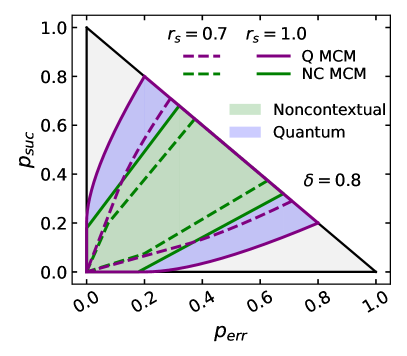
Figure 1: Space of probabilities corresponding to a two-state discrimination setting. Continuous lines denote maximum confidence measurements in both quantum (purple) and noncontextual (green) models. Even with a bounded value of noise ($r_{s}=0.7$), the MCM line according to the quantum model falls outside the noncontextual region.

Noncontextual model—. We now outline a non-contextual ontological model for the prepare-and-measure scenario [10, 50, 18]. The system is associated with an ontic state space $\Omega$ in which each point $\lambda$ completely defines all physical properties, i.e. the outcomes of all possible measurements. Each state preparation $x$ samples the ontic state space according to a probability distribution $\mu_{x}(\lambda)$, referred to as the epistemic state. Each measurement is defined by a set of response functions, that is, non-negative functions $\xi_{b}(\lambda)$ over the ontic space, such that $\sum_{b}\xi_{b}(\lambda)=1$ for all $\lambda\in\Omega$. The probability of obtaining the outcome $b$ when state $\mu_{x}$ was prepared is then

$$p(b|x)=\int_{\Omega}d\lambda\ \mu_{x}(\lambda)\xi_{b}(\lambda).$$ (10)

While distinct ontic states can be perfectly discriminated, epistemic states with overlapping distributions cannot. Distinguishability can be quantified in terms of the confusability between two epistemic states $\mu_{x}$ and $\mu_{y}$:

$$c_{xy}:=\int_{\text{supp}\left[\mu_{x}(\lambda)\right]}d\lambda\ \mu_{y}(\lambda)$$ (11)

It is the discrimination of epistemic states which we compare against quantum state discrimination.

Furthermore, we require the ontological model to be preparation-noncontextual. Two preparations are said to be operationally equivalent if they cannot be distinguished by any measurement, and an ontological model is said to be preparation-noncontextual if all operationally equivalent preparations are assigned to the same epistemic state. To impose noncontextuality on the ontological model, we assume the existence of a particular pair of pure states $S:=\left\{\mu_{0},\mu_{1}\right\}$ and complementary states $S^{\perp}:=\left\{\mu_{0}^{\perp},\mu_{1}^{\perp}\right\}$, i.e. $\mu_{x}$ and $\mu_{x}^{\perp}$ have non-overlapping supports $\mu_{x}(\lambda)\mu_{x}^{\perp}(\lambda)=0\,\,\forall\,\lambda$. The pairwise confusability $c_{01}$ of $\mu_{0}$ and $\mu_{1}$ is the same as for $\mu_{0}^{\perp}$ and $\mu_{1}^{\perp}$. Preparation noncontextuality implies that preparing $\mu_{x}$ and $\mu_{x}^{\perp}$ with equal probability for $x=0$ or $x=1$ must be equivalent [18, 10], that is $\frac{1}{2}\mu_{0}+\frac{1}{2}\mu_{0}^{\perp}=\frac{1}{2}\mu_{1}+\frac{1}{2}\mu_{1}^{\perp}$. This statement implies that any pair from the set of states $\{\mu_{0},\mu_{1},\mu_{0}^{\perp},\mu_{1}^{\perp}\}$ are equal on their overlap, i.e.

$$\mu_{0}(\lambda)=\mu_{1}(\lambda)\ \forall\lambda\in\text{supp}\left[\mu_{0}(\lambda)\right]\cup\text{supp}\left[\mu_{1}(\lambda)\right]\,\forall\,\lambda,$$ (12)

and similarly for the other pairs. This, in turn, results in symmetric confusabilities, $c_{01}=c_{10}:=c$. Quantum and noncontextual models can be then compared through $\delta^{2}=c$. The noncontextual model we use in this work can be understood as an attempt to describe quantum theory, and in general it will reproduce some quantum correlations but not all, as we explore below.

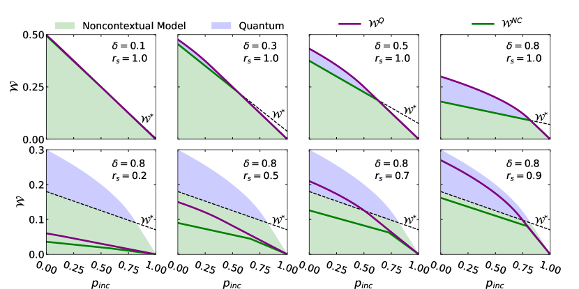
Figure 2: Bounds on the witness $\mathcal{W}$ according to quantum and noncontextual models. On the first row we show noiseless cases with different overlaps. Below, on the second row, we fix a particular overlap and show the effects of depolarising noise on the preparation. The green area denotes the feasible values according to quantum and noncontextual models and the blue region solely for the quantum model. The black-dashed line shows the contextuality witness $\mathcal{W}^{\ast}$ in Eq. (19). Any behavior above $\mathcal{W}^{\ast}$ is an evidence of contextuality.

We now present the main problem in a noncontextual model. The two preparations are represented by the following epistemic states affected by depolarising noise

$$\tilde{\mu}_{0}(\lambda) =r_{s}\mu_{0}(\lambda)+(1-r_{s})\mu_{\mathds{1}/2}(\lambda)$$ (13)

$$\tilde{\mu}_{1}(\lambda) =r_{s}\mu_{1}(\lambda)+(1-r_{s})\mu_{\mathds{1}/2}(\lambda)$$

These can be characterised by the confusability of the noiseless epistemic states $c:=c_{10}$ from Eq. (11). We also consider a single measurement with two conclusive outcomes $b=0,1$ and an inconclusive result $b=ø$, represented by the response functions $\xi_{b}(\lambda)$. Let us define the analogous observable to Eq. (5)

$$\Delta_{x}^{\text{NC}}(\lambda):=\frac{(-1)^{x}}{2}\left(\xi_{0}(\lambda)-\xi_{1}(\lambda)\right)\ .$$ (14)

Then, we can rewrite the problem as a maximisation

$$\mathcal{W}^{\text{NC}}:= \max\frac{1}{2}\left(p^{\text{NC}}_{\text{suc}}-p^{\text{NC}}_{\text{err}}\right)$$ (15)

$$= \max\sum_{x}\int_{\Omega}d\lambda\ \tilde{\mu}_{x}(\lambda)\Delta_{x}^{\text{NC}}(\lambda)\ ,$$

subject to $\xi_{b}(\lambda)$ being valid response functions, $\xi_{b}(\lambda)\geq 0$ and $\sum_{b}\xi_{b}(\lambda)=1$, $\forall\lambda$, and a given rate of inconclusive events $p_{\text{inc}}=\frac{1}{2}\int d\lambda\left(\tilde{\mu}_{0}(\lambda)+\tilde{\mu}_{1}(\lambda)\right)\xi_{ø}(\lambda)$. In [45] we show how this maximisation can be rendered as a simple linear problem, for which we are able to find an analytical solution

$$\mathcal{W}^{\text{NC}} =r_{s}\left(1-c\right)\left(1-\frac{p_{\text{inc}}}{1+r_{s}c}\right)\quad\text{for}\ p_{\text{inc}}\leq(1+r_{s}c)/2$$

$$\mathcal{W}^{\text{NC}} =(1-p_{\text{inc}})\frac{r_{s}(1-c)}{1-r_{s}c}\quad\text{for}\ p_{\text{inc}}\geq(1+r_{s}c)/2\ .$$ (16)

This results in the following success and error probabilities. For $p_{\text{inc}}\leq(1+r_{s}c)/2$

$$p^{\text{NC}}_{\text{suc}} =\frac{1+r_{s}}{2}\left(1-\frac{p_{\text{inc}}}{1+r_{s}c}\right)-\frac{r_{s}c}{2}\ ,$$ (17)

and for $p_{\text{inc}}\geq(1+r_{s}c)/2$

$$p^{\text{NC}}_{\text{suc}} =\frac{1}{2}\left(1+\mathcal{W}^{\text{NC}}-p_{\text{inc}}\right)\ ,$$ (18)

and $p_{\text{err}}^{\text{NC}}=1-p_{\text{suc}}^{\text{NC}}-p_{\text{inc}}$.

Results—. Fig. 1 shows the achievable probabilities in quantum and noncontectual models. The white region delimited by the black contour shows the feasible space in the case of fully distinguishable preparations. That is, when states can be directly identified with ontic states $\lambda$. The area shaded in blue shows the feasible space according to quantum theory. In its contour we find $p_{\text{suc}}^{\text{Q}}$ from Eq. (8), for $r_{s}=1$. The region reproducible by the noncontextual model (green area) is contained in the quantum set. Similarly, we find $p_{\text{suc}}^{\text{NC}}$, from Eq. (17), in its contour, also for $r_{s}=1$. Both the quantum and noncontextual feasible space shrink with increasing overlap $\delta=\sqrt{c}$. We see that the quantum predictions depart from classical (noncontextual) interpretations.

Moreover, we can identify some extremes of the quantum region with the bounds found in each state discrimination protocol. The diagonal line that delimits the upper-right part of the feasible regions covers the state discrimination scenarios with zero inconclusive rates. The vertices of the quantum region on that line reproduce the Helstrom bound [51, 46, 52] obtained in MESD. The same applies for the vertices corresponding to the noncontextual line, which reproduce the maximal success probabilities in MESD obtained in [18]. Also, the maximal $p_{\text{err}}$ and $p_{\text{suc}}$ on the flat part of the bottom and left-most boundary, respectively, reproduce the maximal unambiguous error and success rates for quantum [35] and noncontextual [19] models, obtained in USD. Finally, the entire quantum boundary (purple line) corresponds to a maximum confidence measurement (MCM)[39, 53] for the ensemble of qubit states (i.e. maximising the average confidence). MCM thus provides optimal success probability in any (qubit-)state discrimination scenario. Similarly, the noncontextual boundary is obtained by a noncontextual MCM. We can see, by writing $C=p_{\text{suc}}/(p_{\text{suc}}+p_{\text{err}})$, that the confidence coincides with the bounds found in the literature [39, 40, 38, 53, 19].

When depolarizing is included, the bounds on all protocols depart from the borders of the quantum region. The Helstrom bound from both quantum and noncontextual MESD comes closer to the center of the probability space as noise increases. Also, when noise is taken into account, USD is not possible as here we can see that the bottom and left-most borders are not reachable. The space enclosed by the MCM lines also narrows. For a given noisy ensemble, the points on the quantum region outside the MCM lines are not accessible.

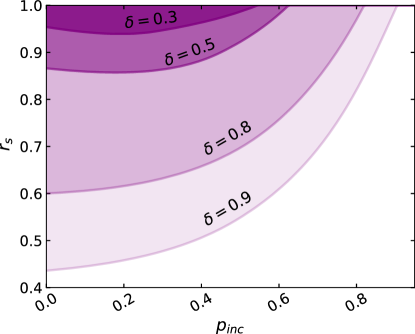
Figure 3: Tolerable amount of depolarising noise for which our witness can detect quantum contextuality as function of inconclusive rate $p_{\text{inc}}$ for different overlaps $\delta$. Contextuality is witnessed in the shaded regions above the solid lines (larger $r_{s}$ means less noise).

A different perspective is plotted in Fig. 2. Contextual behavior is manifested in the blue shaded region above the dashed black line, which corresponds to the inequality

$$\mathcal{W}\leq\mathcal{W}^{*}=\left.\mathcal{W}^{\text{NC}}\right|_{r_{s}=1}=\frac{1-\delta^{2}}{2}\left(1-\frac{p_{\text{inc}}}{1+\delta^{2}}\right)$$ (19)

for noiseless preparations with distinguishability bounded by overlap $\delta$ (quantum) or confusability $\delta^{2}$ (noncontextual). Here, $\mathcal{W}^{*}$ is the noncontextual bound without noise. Note that it is sufficient to lower-bound the confusability (or equivalently the overlap) because our bounds on $\mathcal{W}$ decrease as preparations become less distinguishable. Also, note that the witness places no assumptions on the measurement, which is completely uncharacterised. We see, from the two lower-right plots in Fig. 2 that noncontextuality can be witnessed in the presence of noise.

We finally look at the amount of depolarising noise that our witness can tolerate while still being able to detect contextuality. Depolarising noise in the preparation is parameterized through $r_{s}$ (see above Eq. (5)). In Fig. 3 we show the minimum tolerable $r_{s}$ for which contextuality can be witnessed, i.e. for which $\mathcal{W}^{\rm Q}\geq\mathcal{W}^{*}$. Two noiseless preparations with confusability $c=\delta^{2}$ in a noncontextual model can reproduce all quantum correlations from a two-state discrimination scenario with fixed $p_{\rm inc}$, as long as $r_{s}$ is below the plotted lines. Noise tolerance is higher for larger confusabilities. The cases with null inconclusive outcomes are covered in Refs.[18, 54]. Remarkably, observe that in some cases, the appearance of inconclusive events strengthens robustness, as is e.g. the case for $\delta=0.3$ or $\delta=0.5$ in Fig. 3.

Conclusion.— We presented a witness of contextuality in two-state discrimination scenarios. We started by formulating the problem of finding the optimal measurement in two-state discrimination settings allowing for inconclusive events and found that maximum-confidence meaurements are optimal in both quantum and noncontextual models. That led to the definition of the witness $\mathcal{W}$ in Eq. (4) and the inequality Eq. (19). This inequality allows for a flexible rate of inconclusive events (e.g. due to losses) and is robust against depolarising noise.

We gratefully acknowledge support from the Danish National Research Foundation, Center for Macroscopic Quantum States (bigQ, DNRF142), VILLUM FONDEN (research grant 40864), the Carlsberg Foundation CF19-0313, and a DTU-KAIST Alliance Stipend.

Appendix A Supplemental material: Optimal measurements

In this part of the supplemental material, we derive the optimal measurements for both the quantum and noncontextual models considered in the main text. We call a measurement optimal when it maximises the probability success whilst the error probability is kept at minimum.

A.1 Quantum model

Let us start by writing the semi-definite program that finds the optimal measurement according to the quantum theory. We express the difference we aim to maximise as

$$\mathcal{W}^{\text{Q}}=\frac{1}{2}\left(p_{\text{suc}}^{\text{Q}}-p_{\text{err}}^{\text{Q}}\right) =\frac{1}{2}\left(\operatorname{Tr}\left[\rho_{0}\hat{\pi}_{0}\right]+\operatorname{Tr}\left[\rho_{1}\hat{\pi}_{1}\right]\right)-\frac{1}{2}\left(\operatorname{Tr}\left[\rho_{0}\hat{\pi}_{1}\right]+\operatorname{Tr}\left[\rho_{1}\hat{\pi}_{0}\right]\right)$$

$$=\frac{1}{2}\operatorname{Tr}\left[(\rho_{0}-\rho_{1})(\hat{\pi}_{0}-\hat{\pi}_{1})\right]=\sum_{x=0}^{1}\operatorname{Tr}\left[\rho_{x}\hat{\Delta}_{x}\right]\ ,$$ (20)

where we included the operator $\hat{\Delta}_{x}$ introduced in the main text. One can write down the problem in the following SDP form:

$$\underset{\left\{\hat{\pi}_{b}\right\}}{\text{maximise}} \quad\frac{1}{2}\operatorname{Tr}\left[\rho_{x}\hat{\Delta}_{x}\right]$$

subject  to: $$\quad\hat{\pi}_{b}\geq 0\quad\sum_{b}\hat{\pi}_{b}=\mathds{1}$$ (21)

$$\quad\frac{1}{2}\operatorname{Tr}\left[(\rho_{0}+\rho_{1})\hat{\pi}_{ø}\right]=p_{\text{inc}}$$

We begin by analysing the optimality conditions of the POVM $\hat{\pi}_{b}$. The corresponding Lagrangian is given by

$$\mathcal{L} =\frac{1}{2}\operatorname{Tr}\left[(\rho_{0}-\rho_{1})(\hat{\pi}_{0}-\hat{\pi}_{1})\right]+\sum_{b}r_{b}\operatorname{Tr}\left[\hat{\pi}_{b}\sigma_{b}\right]+\operatorname{Tr}\left[K\left(\mathds{1}-\sum_{b}\hat{\pi}_{b}\right)\right]+s\left(p_{\text{inc}}-\frac{1}{2}\operatorname{Tr}\left[(\rho_{0}+\rho_{1})\hat{\pi}_{ø}\right]\right)\ ,$$ (22)

where we introduced the following dual variables: $r_{b}\sigma_{b}$ for the PSD constraint, $K$ accounting for the normalisation constraint and $s$ for the constraint fixing the inconclusive rate. The dual problem can be straight formulated through the supremum of the Lagrangian

$$\mathcal{S}=\underset{\hat{\pi}_{b}}{\text{supp}}\ \operatorname{Tr}\left[K\right]+sp_{\text{inc}}+\sum_{b}\operatorname{Tr}\left[\hat{\pi}_{b}G_{b}\right]\ ,$$ (23)

where we defined

$$G_{b} =\frac{1}{2}\operatorname{Tr}\left[\left(\rho_{0}-\rho_{1}\right)\left(\delta_{b,0}-\delta_{b,1}\right)\right]+r_{b}\sigma_{b}-\frac{1}{2}\left(\rho_{0}+\rho_{1}\right)\delta_{b,ø}-K\ .$$ (24)

The supremum in Eq. (23) will diverge unless $G_{b}=0$. This leads to the Lagrange Stability optimality condition. Complementary slackness reads $r_{b}\operatorname{Tr}\left[\sigma_{b}\hat{\pi}_{b}\right]=0$, which in a qubit space means that $\pi_{b}$ must be rank-1. With all that, we are ready to derive the form of the optimal POVM. We consider a pair of pure states $\rho_{x}$ oriented symmetrically with respect to the $Z$ pole in the Bloch sphere. That means

$$\rho_{0}=\frac{1}{2}\left[\mathds{1}+r\sqrt{1-\delta^{2}}X+r_{s}\delta Z\right]\quad,\qquad\rho_{1}=\frac{1}{2}\left[\mathds{1}-r_{s}\sqrt{1-\delta^{2}}X+r\delta Z\right]\ .$$ (25)

By fixing the orientation of the states in that way, the problem acquires a symmetry with respect to the states. This is very convenient since we can directly find the analytical form of $\hat{\pi}_{ø}$ through the last constraint in Eq. (A.1): $\hat{\pi}_{ø}=\frac{p_{\text{inc}}}{1+r_{s}\delta}\left[\mathds{1}+Z\right]$. The other two POVM elements ($\hat{\pi}_{0}$ and $\hat{\pi}_{1}$) can be also directly found noting that the maximum in Eq. (A.1) is reached when $\hat{\pi}_{0}-\hat{\pi}_{1}$ is proportional to $\rho_{0}-\rho_{1}=r_{s}\sqrt{1-\delta^{2}}X$ (according to Eq. (25)). At the end of the day, this leaves us with the following optimal POVM:

$$\hat{\pi}_{0}= \frac{1}{2}\left(1-\frac{p_{\text{inc}}}{1+r_{s}\delta}\right)\left[\mathds{1}+\frac{1+r_{s}\delta}{r_{s}\sqrt{1-\delta^{2}}}\frac{\mathcal{W}^{\text{Q}}}{1+r_{s}\delta-p_{\text{inc}}}X-\frac{p_{\text{inc}}}{1+r_{s}\delta-p_{\text{inc}}}Z\right]$$ (26)

$$\hat{\pi}_{1}= \frac{1}{2}\left(1-\frac{p_{\text{inc}}}{1+r_{s}\delta}\right)\left[\mathds{1}-\frac{1+r_{s}\delta}{r\sqrt{1-\delta^{2}}}\frac{\mathcal{W}^{\text{Q}}}{1+r_{s}\delta-p_{\text{inc}}}X-\frac{p_{\text{inc}}}{1+r_{s}\delta-p_{\text{inc}}}Z\right]$$ (27)

$$\hat{\pi}_{ø}= \frac{2Q}{1+r_{s}\delta}\frac{1}{2}\left[\mathds{1}+Z\right]\ ,$$ (28)

for $p_{\text{inc}}\leq r_{s}\delta$, and

$$\hat{\pi}_{0}= \frac{1}{2}\frac{1-p_{\text{inc}}}{1-r_{s}^{2}\delta^{2}}\left[\mathds{1}+\sqrt{1-r_{s}^{2}\delta^{2}}X-r_{s}\delta Z\right]$$ (29)

$$\hat{\pi}_{1}= \frac{1}{2}\frac{1-p_{\text{inc}}}{1-r_{s}^{2}\delta^{2}}\left[\mathds{1}-\sqrt{1-r_{s}^{2}\delta^{2}}X-r_{s}\delta Z\right]$$ (30)

$$\hat{\pi}_{ø}= \frac{2(p_{\text{inc}}-r_{s}^{2}\delta^{2})}{1-r_{s}^{2}\delta^{2}}\frac{1}{2}\left[\mathds{1}+\frac{1-p_{\text{inc}}}{p_{\text{inc}}-r_{s}^{2}\delta^{2}}Z\right]\ ,$$ (31)

for $p_{\text{inc}}\geq r_{s}\delta$. That POVM yields the optimal measurement that maximises the difference between success and error probabilities for a fixed rate of inconclusive events.

A.2 Noncontextual model

In a noncontextual model we can write the problem in the following maximisation form:

$$\underset{\xi_{b}(\lambda)}{\text{maximise}} \quad\frac{1}{2}\int d\lambda\left(\tilde{\mu}_{0}(\lambda)-\tilde{\mu}_{1}(\lambda)\right)\left(\xi_{0}(\lambda)-\xi_{1}(\lambda)\right)$$ (32)

subject to: $$\quad\xi_{b}(\lambda)\geq 0,\ \sum_{b}\xi_{b}(\lambda)=1\ \forall\lambda$$

$$\quad p_{\text{inc}}=\frac{1}{2}\int d\lambda\left(\tilde{\mu}_{0}(\lambda)+\tilde{\mu}_{1}(\lambda)\right)\xi_{ø}(\lambda)\ .$$

We consider a pair of noisy epistemic states affected by depolarising noise:

$$\tilde{\mu}_{0}(\lambda)=r_{s}\mu_{0}(\lambda)+(1-r_{s})\mu_{\mathds{1}/2}(\lambda)\quad,\qquad\tilde{\mu}_{1}(\lambda)=r_{s}\mu_{1}(\lambda)+(1-r_{s})\mu_{\mathds{1}/2}(\lambda)\ .$$ (33)

These are characterised by the confusability of the noiseless states given by

$$c_{10}=\int_{\text{supp}\left[\mu_{0}(\lambda)\right]}d\lambda\mu_{1}(\lambda)\ .$$ (34)

For low enough rates of inconclusive events, the optimal response functions are those which unambiguously discriminate the noiseless epistemic states. These are of the following form

$$\xi_{0}(\lambda)=\begin{cases}q&\mbox{if }\lambda\in{\rm supp}[\overline{\mu}_{1}(\lambda)]\\ 0&\mbox{otherwise }\ .\end{cases}\quad\xi_{1}(\lambda)=\begin{cases}q&\mbox{if }\lambda\in{\rm supp}[\overline{\mu}_{0}(\lambda)]\\ 0&\mbox{otherwise }\ .\end{cases}$$ (35)

One can determine the value of $q$ in terms of the rate of inconclusive events and obtain

$$q=\frac{1-p_{\text{inc}}}{1-r_{s}c_{10}}$$ (36)

leaving the following extremal success and error probabilities:

$$p_{\text{suc}}^{\text{NC}}=\frac{1-p_{\text{inc}}}{2}\left(1+\frac{r_{s}(1-c_{10})}{1-r_{s}c_{10}}\right)\quad p_{\text{err}}^{\text{NC}}=\frac{1-r_{s}}{2}\frac{1-p_{\text{inc}}}{1-r_{s}c_{10}}\ .$$ (37)

Normalisation implies in Eq. (36) that $p_{\text{inc}}\geq(1+r_{s}c_{10})/2$. In the noiseless case, that is the lower bound on the rate of inconclusive events in USD. Also, note that the confidence can be written as $C=p_{\text{suc}}/(1-p_{\text{inc}})$, which according to Eq. (37) one recovers the maximum confidence in [19] according to a noncontextual model.

For smaller rates $p_{\text{inc}}$, the support of the response functions corresponding to conclusive outcomes will shift to the support of the oposite states. In other words, we can write down these response functions as follows

$$\xi_{0}(\lambda)=\begin{cases}a&\mbox{if }\lambda\in{\rm supp}[\mu_{0}(\lambda)]\cup{\rm supp}[\overline{\mu}_{1}(\lambda)]\\ b&\mbox{if }\lambda\in{\rm supp}[\overline{\mu}_{0}(\lambda)]\cup{\rm supp}[\overline{\mu}_{1}(\lambda)]\\ a-b&\mbox{if }\lambda\in{\rm supp}[\mu_{0}(\lambda)]\cup{\rm supp}[\mu_{1}(\lambda)]\\ 0&\text{otherwise}\end{cases}$$ (38)

$$\xi_{1}(\lambda)=\begin{cases}a&\mbox{if }\lambda\in{\rm supp}[\overline{\mu}_{0}(\lambda)]\cup{\rm supp}[\mu_{1}(\lambda)]\\ b&\mbox{if }\lambda\in{\rm supp}[\overline{\mu}_{0}(\lambda)]\cup{\rm supp}[\overline{\mu}_{1}(\lambda)]\\ a-b&\mbox{if }\lambda\in{\rm supp}[\mu_{0}(\lambda)]\cup{\rm supp}[\mu_{1}(\lambda)]\\ 0&\text{otherwise}\end{cases}\ .$$ (39)

Note that if $a=b$ we recover the response functions in Eq. (35). This allows us to rewrite the initial optimisation problem Eq. (32) in the following form

$$\underset{a,b}{\text{maximise}} \quad\frac{1}{2}ar_{s}(1-c_{10})$$ (40)

subject to $$\quad a-b\leq 2\ ,\quad b\leq\frac{1}{2}$$ (41)

$$\quad p_{\text{inc}}=1-a(1+r_{s}c_{10})+2br_{s}c_{10}\ .$$ (42)

The optimal values of the parameters $a$ and $b$ are

$$a=1-\frac{p_{\text{inc}}}{1+r_{s}c_{10}}\quad b=\frac{1}{2}\ .$$ (43)

Then, one can write the success and error probabilities directly as follows:

$$p_{\text{suc}}^{\text{NC}} =\frac{1+r_{s}}{2}\left(1-\frac{p_{\text{inc}}}{1+r_{s}c_{10}}\right)-\frac{r_{s}c_{10}}{2}$$ (44)

$$p_{\text{err}}^{\text{NC}} =\left(r_{s}c_{10}+\frac{1-r_{s}}{2}\right)\left(1-\frac{p_{\text{inc}}}{1+r_{s}c_{10}}\right)-\frac{r_{s}c_{10}}{2}\ .$$ (45)

One can use this result to obtain the maximum confidence for smaller inconclusive rates (i.e. for $p_{\text{inc}}\leq(1+rc_{10})/2$), which yields

$$\max C^{\text{NC}}=\frac{1}{2(1-p_{\text{inc}})}\left((1+r_{s})\left(1-\frac{p_{\text{inc}}}{1+r_{s}c_{10}}\right)-rc_{10}\right)$$ (46)

We can claim that this is the maximum confidence since it is also achieved by a measurement that simultaneously minimizes the error and maximises the success.

References

- Kochen and Specker [1968] S. Kochen and E. Specker, The problem of hidden variables in quantum mechanics, Indiana Univ. Math. J. 17, 59 (1968).
- Bell [1966] J. S. Bell, On the problem of hidden variables in quantum mechanics, Rev. Mod. Phys. 38, 447 (1966).
- Howard et al. [2014] M. Howard, J. Wallman, V. Veitch, and J. Emerson, Contextuality supplies the ‘magic’for quantum computation, Nature 510, 351 (2014).
- Bechmann-Pasquinucci and Peres [2000] H. Bechmann-Pasquinucci and A. Peres, Quantum cryptography with 3-state systems, Phys. Rev. Lett. 85, 3313 (2000).
- Horodecki et al. [2010] K. Horodecki, M. Horodecki, P. Horodecki, R. Horodecki, M. Pawlowski, and M. Bourennane, Contextuality offers device-independent security (2010), arXiv:1006.0468 [quant-ph] .
- Abbott et al. [2012] A. A. Abbott, C. S. Calude, J. Conder, and K. Svozil, Strong kochen-specker theorem and incomputability of quantum randomness, Phys. Rev. A 86, 062109 (2012).
- Chailloux et al. [2016] A. Chailloux, I. Kerenidis, S. Kundu, and J. Sikora, Optimal bounds for parity-oblivious random access codes, New Journal of Physics 18, 045003 (2016).
- Klyachko et al. [2008] A. A. Klyachko, M. A. Can, S. Binicioğlu, and A. S. Shumovsky, Simple test for hidden variables in spin-1 systems, Phys. Rev. Lett. 101, 020403 (2008).
- Cabello et al. [2013] A. Cabello, P. Badzia¸g, M. Terra Cunha, and M. Bourennane, Simple hardy-like proof of quantum contextuality, Phys. Rev. Lett. 111, 180404 (2013).
- Spekkens [2005] R. W. Spekkens, Contextuality for preparations, transformations, and unsharp measurements, Phys. Rev. A 71, 052108 (2005).
- Spekkens et al. [2009] R. W. Spekkens, D. H. Buzacott, A. J. Keehn, B. Toner, and G. J. Pryde, Preparation contextuality powers parity-oblivious multiplexing, Phys. Rev. Lett. 102, 010401 (2009).
- Ghorai and Pan [2018] S. Ghorai and A. K. Pan, Optimal quantum preparation contextuality in an -bit parity-oblivious multiplexing task, Phys. Rev. A 98, 032110 (2018).
- Ambainis et al. [2019] A. Ambainis, M. Banik, A. Chaturvedi, D. Kravchenko, and A. Rai, Parity oblivious d-level random access codes and class of noncontextuality inequalities, Quantum Information Processing 18, 111 (2019).
- Roch i Carceller et al. [2022] C. Roch i Carceller, K. Flatt, H. Lee, J. Bae, and J. B. Brask, Quantum vs noncontextual semi-device-independent randomness certification, Phys. Rev. Lett. 129, 050501 (2022).
- Hameedi et al. [2017] A. Hameedi, A. Tavakoli, B. Marques, and M. Bourennane, Communication games reveal preparation contextuality, Phys. Rev. Lett. 119, 220402 (2017).
- Saha et al. [2019] D. Saha, P. Horodecki, and M. Pawłowski, State independent contextuality advances one-way communication, New Journal of Physics 21, 093057 (2019).
- Saha and Chaturvedi [2019] D. Saha and A. Chaturvedi, Preparation contextuality as an essential feature underlying quantum communication advantage, Phys. Rev. A 100, 022108 (2019).
- Schmid and Spekkens [2018] D. Schmid and R. W. Spekkens, Contextual advantage for state discrimination, Phys. Rev. X 8, 011015 (2018).
- Flatt et al. [2022] K. Flatt, H. Lee, C. Roch i Carceller, J. B. Brask, and J. Bae, Contextual advantages and certification for maximum-confidence discrimination, PRX Quantum 3, 030337 (2022).
- Banik et al. [2015] M. Banik, S. S. Bhattacharya, A. Mukherjee, A. Roy, A. Ambainis, and A. Rai, Limited preparation contextuality in quantum theory and its relation to the cirel’son bound, Phys. Rev. A 92, 030103 (2015).
- Krishna et al. [2017] A. Krishna, R. W. Spekkens, and E. Wolfe, Deriving robust noncontextuality inequalities from algebraic proofs of the kochen–specker theorem: the peres–mermin square, New Journal of Physics 19, 123031 (2017).
- Kunjwal and Spekkens [2015] R. Kunjwal and R. W. Spekkens, From the kochen-specker theorem to noncontextuality inequalities without assuming determinism, Phys. Rev. Lett. 115, 110403 (2015).
- Kunjwal and Spekkens [2018] R. Kunjwal and R. W. Spekkens, From statistical proofs of the kochen-specker theorem to noise-robust noncontextuality inequalities, Phys. Rev. A 97, 052110 (2018).
- Mazurek et al. [2016] M. D. Mazurek, M. F. Pusey, R. Kunjwal, K. J. Resch, and R. W. Spekkens, An experimental test of noncontextuality without unphysical idealizations, Nature Communications 7, ncomms11780 (2016).
- Pusey [2018] M. F. Pusey, Robust preparation noncontextuality inequalities in the simplest scenario, Phys. Rev. A 98, 022112 (2018).
- Schmid et al. [2018] D. Schmid, R. W. Spekkens, and E. Wolfe, All the noncontextuality inequalities for arbitrary prepare-and-measure experiments with respect to any fixed set of operational equivalences, Phys. Rev. A 97, 062103 (2018).
- Bae et al. [2016] J. Bae, D.-G. Kim, and L.-C. Kwek, Structure of optimal state discrimination in generalized probabilistic theories, Entropy 18, 10.3390/e18020039 (2016).
- Kimura et al. [2009] G. Kimura, T. Miyadera, and H. Imai, Optimal state discrimination in general probabilistic theories, Phys. Rev. A 79, 062306 (2009).
- Barnett and Croke [2009] S. M. Barnett and S. Croke, Quantum state discrimination, Adv. Opt. Photon. 1, 238 (2009).
- Bae and Kwek [2015] J. Bae and L.-C. Kwek, Quantum state discrimination and its applications, Journal of Physics A: Mathematical and Theoretical 48, 083001 (2015).
- Bergou [2007] J. A. Bergou, Quantum state discrimination and selected applications, Journal of Physics: Conference Series 84, 012001 (2007).
- Loubenets [2022] E. R. Loubenets, General lower and upper bounds under minimum-error quantum state discrimination, Phys. Rev. A 105, 032410 (2022).
- Bae [2013] J. Bae, Structure of minimum-error quantum state discrimination, New Journal of Physics 15, 073037 (2013).
- Herzog [2004] U. Herzog, Minimum-error discrimination between a pure and a mixed two-qubit state, Journal of Optics B: Quantum and Semiclassical Optics 6, S24 (2004).
- Ivanovic [1987] I. D. Ivanovic, How to differentiate between non-orthogonal states, Physics Letters A 123, 257 (1987).
- Dieks [1988] D. Dieks, Overlap and distinguishability of quantum states, Physics Letters A 126, 303 (1988).
- Peres [1988] A. Peres, How to differentiate between non-orthogonal states, Physics Letters A 128, 19 (1988).
- Jiménez et al. [2011] O. Jiménez, M. A. Solís-Prosser, A. Delgado, and L. Neves, Maximum-confidence discrimination among symmetric qudit states, Phys. Rev. A 84, 062315 (2011).
- Croke et al. [2006] S. Croke, E. Andersson, S. M. Barnett, C. R. Gilson, and J. Jeffers, Maximum confidence quantum measurements, Phys. Rev. Lett. 96, 070401 (2006).
- Herzog [2009] U. Herzog, Discrimination of two mixed quantum states with maximum confidence and minimum probability of inconclusive results, Phys. Rev. A 79, 032323 (2009).
- Herzog [2012] U. Herzog, Optimized maximum-confidence discrimination of mixed quantum states and application to symmetric states, Phys. Rev. A 85, 032312 (2012).
- Herzog [2015] U. Herzog, Optimal measurements for the discrimination of quantum states with a fixed rate of inconclusive results, Phys. Rev. A 91, 042338 (2015).
- Bagan et al. [2012] E. Bagan, R. Muñoz Tapia, G. A. Olivares-Rentería, and J. A. Bergou, Optimal discrimination of quantum states with a fixed rate of inconclusive outcomes, Phys. Rev. A 86, 040303 (2012).
- Vandenberghe and Boyd [1996] L. Vandenberghe and S. Boyd, Semidefinite programming, SIAM Review 38, 49 (1996), https://doi.org/10.1137/1038003 .
- i Carceller and Brask [2023] C. R. i Carceller and J. B. Brask, Supplemental material for: A contextuality witness inspired by optimal state discrimination, (2023).
- Helstrom [1968] C. W. Helstrom, Detection theory and quantum mechanics (ii), Information and Control 13, 156 (1968).
- Qiu [2008] D. Qiu, Minimum-error discrimination between mixed quantum states, Phys. Rev. A 77, 012328 (2008).
- Kleinmann et al. [2010] M. Kleinmann, H. Kampermann, and D. Bruß, Unambiguous discrimination of mixed quantum states: Optimal solution and case study, Phys. Rev. A 81, 020304 (2010).
- Salazar and Delgado [2012] R. Salazar and A. Delgado, Quantum tomography via unambiguous state discrimination, Phys. Rev. A 86, 012118 (2012).
- Spekkens [2008] R. W. Spekkens, Negativity and contextuality are equivalent notions of nonclassicality, Phys. Rev. Lett. 101, 020401 (2008).
- Helstrom [1967] C. W. Helstrom, Detection theory and quantum mechanics, Information and Control 10, 254 (1967).
- Helstrom [1969] C. W. Helstrom, Quantum detection and estimation theory, Journal of Statistical Physics 1, 231 (1969).
- Lee et al. [2022] H. Lee, K. Flatt, C. Roch i Carceller, J. B. Brask, and J. Bae, Maximum-confidence measurement for qubit states, Phys. Rev. A 106, 032422 (2022).
- Rossi et al. [2023] V. P. Rossi, D. Schmid, J. H. Selby, and A. B. Sainz, Contextuality with vanishing coherence and maximal robustness to dephasing (2023), arXiv:2212.06856 [quant-ph] .