CatNorth: An Improved Gaia DR3 Quasar Candidate Catalog with Pan-STARRS1 and CatWISE

Abstract

A complete and pure sample of quasars with accurate redshifts is crucial for quasar studies and cosmology. In this paper, we present CatNorth, an improved Gaia DR3 quasar candidate catalog with more than 1.5 million sources in the 3$\pi$ sky built with data from Gaia, Pan-STARRS1, and CatWISE2020. The XGBoost algorithm is used to reclassify the original Gaia DR3 quasar candidates as stars, galaxies, and quasars. To construct training/validation datasets for the classification, we carefully built two different master stellar samples in addition to the spectroscopic galaxy and quasar samples. An ensemble classification model is obtained by averaging two XGBoost classifiers trained with different master stellar samples. Using a probability threshold of $p_{\mathrm{QSO\_mean}}>0.95$ in our ensemble classification model and an additional cut on the logarithmic probability density of zero proper motion, we retrieved 1,545,514 reliable quasar candidates from the parent Gaia DR3 quasar candidate catalog. We provide photometric redshifts for all candidates with an ensemble regression model. For a subset of 89,100 candidates, accurate spectroscopic redshifts are estimated with the Convolutional Neural Network from the Gaia BP/RP spectra. The CatNorth catalog has a high purity of $\sim 90\%$ while maintaining high completeness, which is an ideal sample to understand the quasar population and its statistical properties. The CatNorth catalog is used as the main source of input catalog for the LAMOST phase III quasar survey, which is expected to build a highly complete sample of bright quasars with $i<19.5$.

1 Introduction

Quasars are luminous Active Galactic Nuclei (AGNs) with supermassive black holes at their centers that release huge amounts of energy through accreting surrounding gaseous materials. Found from the nearby to the distant universe, quasars are important in various aspects of astronomy. With especially massive black holes of up to $\sim 10$ billion solar masses at high redshifts (see e.g. Wu et al., 2015; Bañados et al., 2018; Fan et al., 2023), quasars are key to understanding the formation and evolution of supermassive black holes, and the association between black holes and host galaxies (e.g. Di Matteo et al., 2005; Kormendy & Ho, 2013). The absorption lines of quasars can trace the interstellar and intergalactic medium at different redshifts (e.g. Weymann et al., 1981; Rees, 1986; Trump et al., 2006). A large sample of quasars can reveal the large-scale structure of the Universe (e.g. Eisenstein et al., 2011; Dawson et al., 2013; Blanton et al., 2017). Furthermore, quasars are ideal objects for defining celestial reference frames, because they are distant point sources with small parallaxes and proper motions (e.g. Ma et al., 2009; Mignard et al., 2016; Gaia Collaboration et al., 2018, 2022).

Recently, bright quasars have also shown the potential to determine the expansion history of the Universe with the Sandage test (Sandage, 1962; Liske et al., 2008; Cristiani et al., 2023). In addition, quasars that are bright in the UV and X-ray can also serve as high-redshift standard candles to constrain the cosmological models using the $L_{\rm X}-L_{\rm UV}$ relation (e.g. Risaliti & Lusso, 2015, 2019).

The sixteenth data release of the Sloan Digital Sky Survey Quasar Catalog (SDSS DR16Q; Lyke et al., 2020) is the largest quasar catalog to date, which contains data for 750,414 quasars that are spectroscopically identified from SDSS-I to SDSS-IV. Parallel to the SDSS quasar survey, the LAMOST quasar survey has observed 56,175 quasars in the first nine years of the regular survey, of which 31,866 were independently discovered by LAMOST (Ai et al., 2016; Dong et al., 2018; Yao et al., 2019; Jin et al., 2023).

Recently, Gaia DR3 (GDR3; Gaia Collaboration et al., 2023a) announced a sample of 6.6 million candidate quasars (the qso_candidates table, hereafter the GDR3 QSO candidate catalog; Gaia Collaboration et al., 2023b), of which 162,686 have publicly available low-resolution BP/RP spectra. The GDR3 QSO candidate catalog has high completeness thanks to the combination of several different classification modules, including the Discrete Source Classifier (DSC), the Quasar Classifier (QSOC), the variability classification module, the surface brightness profile module, and the Gaia DR3 Celestial Reference Frame source table. Nevertheless, the GDR3 QSO candidate catalog has a low purity of quasars (52%) and a large scatter of redshift estimates, which may limit the application of the sample in quasar and cosmological studies.

To obtain purer subsamples from the GDR3 QSO candidate catalog, some recipes have been suggested by Gaia Collaboration et al. (2023b) and works that use external data such as UnWISE (Storey-Fisher et al., 2023). Storey-Fisher et al. (2023) obtained the “Quaia” catalog with 1,295,502 sources at $G<20.5$ by applying cuts on colors and proper motions to remove non-quasar contaminants (stars and galaxies). Although a model of Quaia’s selection function on sky positions is given by Storey-Fisher et al. (2023), the selection effects introduced by the color cuts are not quantified. While simple color cuts can get high completeness and purity of $\sim 96\%$ for quasar selection at the bright end (e.g. $\mathrm{W1-W2>0.2}$ mag at $G_{\mathrm{BP}}<17$ mag; Onken et al., 2023), they are inadequate to disentangle different classes of objects that overlap with each other in two-dimensional color spaces at fainter magnitudes such as $G=20.5$ or the Gaia magnitude limit of 21 mag. Also, color cuts reduce the sample completeness because they inherit selection biases from the labeled samples (e.g. SDSS quasars).

The original redshift estimates of GDR3 QSO candidates are derived by matching the BP/RP spectra with a set of template spectra of quasars. Although pretty precise for sources with good BP/RP spectra, the Gaia redshift has a large outlier fraction due to the misidentification of emission lines (De Angeli et al., 2023). To improve the overall accuracy of redshift estimates of the GDR3 QSO candidates, Storey-Fisher et al. (2023) trained a $k$-Nearest Neighbors ($k$-NN) model on a subset of Quaia with SDSS redshifts. The $k$-NN model takes photometric data from Gaia and UnWISE, and the redshift estimates from Gaia BP/RP spectra as input features.

The Gaia BP/RP spectra have also speeded up the spectroscopic confirmation of bright quasars. For example, Cristiani et al. (2023) obtained secure redshifts for 1,672 confidently classified quasar candidates with $z\gtrsim 2.5$ by fitting their spectral energy distributions (SEDs) with both multiband photometric data and the Gaia DR3 BP/RP spectra. The Cristiani et al. (2023) SED fitting method yields a typical uncertainty of $\sigma_{\mathrm{NMAD}}=0.02$ on 938 quasars with spectroscopic redshifts of $2.5\lesssim z\lesssim 4.0$.

In this work, to select quasars to $G=21$ mag, we choose the machine learning method, which can characterize celestial objects in high-dimensional feature/color spaces. For instance, Nakoneczny et al. (2021) have reported that machine learning methods such as XGBoost can achieve purity of 97% and completeness of 94% at $r<22$ for quasar selection. In a previous paper on finding quasars behind the Galactic plane (Fu et al., 2021), we have also shown the successful application of the machine learning method in selecting quasars with optical data from Pan-STARRS1 and mid-IR data from AllWISE. In addition, we have introduced a cut in the logarithmic probability density of zero proper motion ($\log(f_{\mathrm{PM0}})$) derived from Gaia DR2 data, to further exclude stellar contaminants while retaining more than 99% of the quasars.

With more recent releases of the CatWISE2020 catalog (Marocco et al., 2021) and Gaia DR3, we are now able to build a better classification model with photometric data from Gaia, Pan-STARRS1, and CatWISE, and obtain more accurate $\log(f_{\mathrm{PM0}})$ values with Gaia DR3. In addition, we propose to achieve better quasar redshift measurements in comparison to the original GDR3 QSO candidate catalog and Quaia, with machine learning methods and both multiband photometry and Gaia BP/RP spectra.

The structure of this paper is described below. Section 2 introduces the data sets used in this study. Section 3 discusses feature selection and characterizes different classes of objects in the feature space. Section 4 describes the procedure to build the XGBoost ensemble classification model. Section 5 explores further purification of the quasar candidates using the proper motion data from Gaia DR3. Section 6 describes redshift estimation using machine learning with photometric data and Gaia BP/RP spectra. Section 7 presents the contents and statistical properties of the final CatNorth catalog. The study is summarized in Section 8. Throughout this paper, we adopt a flat $\Lambda$CDM cosmology with $\Omega_{\Lambda}=0.7$, $\Omega_{M}=0.3$ and $H_{0}=70\,\mathrm{km\,s^{-1}\,Mpc^{-1}}$.

2 Data

The input data of this work is the Gaia DR3 quasar candidate catalog (the qso_candidates table) from Gaia Collaboration et al. (2023b) . We combine optical and infrared photometric data from Gaia DR3, Pan-STARRS1 and CatWISE2020, and astrometric data from Gaia DR3 to improve both purity and redshift estimation of the GDR3 QSO candidate catalog. We also retrieve samples of spectroscopically identified extragalactic objects from SDSS and stellar samples from a variety of catalogs to build well-defined training/validation samples.

2.1 Astrometric and photometric data

2.1.1 Gaia DR3 astrometric and astrophysical data

Gaia DR3 (Gaia Collaboration et al., 2023a) contains the same source list, celestial positions, proper motions, parallaxes, and broadband photometry in the G, $G_{\mathrm{BP}}$ (330–680 nm), and $G_{\mathrm{RP}}$ (630–1050 nm) passbands for 1.8 billion sources brighter than magnitude 21 already present in the Early Third Data Release (Gaia EDR3; Gaia Collaboration et al., 2021). Furthermore, the Gaia DR3 catalog incorporates a much expanded radial velocity survey and a very extensive astrophysical characterization of Gaia sources, including about 1 million mean spectra from the radial velocity spectrometer, and about 220 million low-resolution blue and red prism photometer BP/RP mean spectra. The results of the analysis of epoch photometry are provided for about 10 million sources across 24 variability types. Gaia DR3 includes astrophysical parameters and source class probabilities for about 470 million and 1,500 million sources, respectively, including stars, galaxies, and quasars. For a large fraction of the objects, the catalog lists astrophysical parameters (APs) determined from parallaxes, broadband photometry, and the mean Radial Velocity Spectrometer (RVS) or mean BP/RP spectra.

With the new definition of Gaia (E)DR3 passbands (Riello et al., 2021), we calculate the extinction coefficients of $G_{\mathrm{BP}}$, G, and $G_{\mathrm{RP}}$ as $R_{G_{\mathrm{BP}}},R_{G},R_{G_{\mathrm{RP}}}=3.4751,2.8582,1.8755$. These coefficients are calculated using $R_{\lambda}=A_{\lambda}/A_{V}\times R_{V}$, where $A_{\lambda}/A_{V}$ is the relative extinction value for a passband $\lambda$ given by the optical to mid-IR extinction law from Wang & Chen (2019), and $R_{V}=3.1$.

2.1.2 Pan-STARRS1 DR1 photometry

Pan-STARRS1 (PS1; Chambers et al., 2016; STScI, 2022) has carried out a set of synoptic imaging sky surveys including the 3$\pi$ Steradian Survey and the Medium Deep Survey in 5 bands $(grizy_{\mathrm{P1}})$. The mean 5$\sigma$ point source limiting sensitivities in the stacked 3$\pi$ Steradian Survey in $(grizy_{\mathrm{P1}})$ are (23.3, 23.2, 23.1, 22.3, 21.4) and the single epoch 5$\sigma$ depths in $(grizy_{\mathrm{P1}})$ are (22.0, 21.8, 21.5, 20.9, 19.7). The mean coordinates from the PS1 MeanObject table are used for better astrometry. The mean point spread function (PSF) magnitudes are used for all bands $(grizy_{\mathrm{P1}})$. The Galactic extinction coefficients for $(grizy_{\mathrm{P1}})$ are $R_{g},R_{r},R_{i},R_{z},R_{y}=3.5805,2.6133,1.9468,1.5097,1.2245$. These coefficients are also calculated with relative extinction $A_{\lambda}/A_{V}$ values from Wang & Chen (2019).

For simplification, we use ($g,r,i,z,y$) to represent the PSF magnitudes of PS1 bands ($grizy_{\mathrm{P1}}$). The $z_{\mathrm{P1}}$ PSF magnitude does not appear alone and will not be confused with the redshift symbol $z$. We set some constraints on the PS1 data to ensure the quality of the data. All sources should be: (i) significantly detected in the PS1 $i$ band ($i>0$, and $i\_err<0.2171$, equivalent to the S/N ratio of the $i_{\mathrm{P1}}$ band greater than 5); and (ii) not too bright in $i$ to avoid possible saturation ($i>14$). The magnitude limit of sources that meet these constraints is $i\approx 21.5$.

2.1.3 CatWISE2020 catalog

The CatWISE2020 Catalog (Marocco et al., 2021, 2020) consists of 1,890,715,640 sources over the entire sky selected from Wide-field Infrared Survey Explorer (WISE; Wright et al., 2010) and NEOWISE (Mainzer et al., 2011) post-cryogenic survey data at 3.4 and 4.6 $\mu$m (W1 and W2) collected from 2010 January 7 to 2018 December 13. The 90% completeness depth for the CatWISE2020 Catalog is at $\rm W1=17.7$ mag and $\rm W2=17.5$ mag. The Galactic extinction coefficients for W1, and W2 used in this study are $R_{\mathrm{W1}},R_{\mathrm{W2}}=0.1209,0.0806$. These coefficients are also calculated with relative extinction $A_{\lambda}/A_{V}$ values from Wang & Chen (2019).

We cross-match the Gaia DR3 coordinates with CatWISE2020 using a radius of $1^{\prime\prime}$. We also set some constraints on the CatWISE2020 data. All sources should be: (i) not too bright to avoid possible saturation (w1mpro_pm>7 & w2mpro_pm>7); (ii) significantly detected in W1 and W2 bands (w1snr_pm>5 & w2snr_pm>5).

2.2 Stellar samples

In this paper, the selection of quasar candidates is performed through a machine learning classification approach, which requires well-defined samples of different classes of objects, namely quasars, galaxies, and stars. SDSS (York et al., 2000) has provided a rich database of spectroscopically identified quasars and galaxies, which can be representative of extragalactic sources within the detection limit of Gaia ($G\approx 21$) in a considerably large sky area.

While many spectroscopic surveys have also identified a vast number of stars, the build-up of a good stellar sample for machine learning is nontrivial due to the heterogeneity among different stellar subsamples. These subsamples vary in completeness and uncertainty levels of stellar parameters because (i) the samples are selected with different methods, and (ii) their spectra are often fitted with different stellar models.

In order to increase the diversity of the stars and ensure the accuracy of the source labels, we construct two master stellar samples by combining many different catalogs. The first master stellar sample ‘LVAC_PLUS’ is mainly built from two LAMOST value-added catalogs, with an extra sample of MLT dwarfs, white dwarfs, and carbon stars described in Section 2.2.3. The other master stellar sample ‘GDR3_PLUS’ is built primarily from Gaia DR3 data, with the same extra stellar sample as in Section 2.2.3. The subsequent training process will produce two classification models by swapping the two master stellar samples.

The selection criteria for the stellar samples are described as follows.

2.2.1 OBAFGK Stars from LAMOST Value-Added Catalogs

The Large Sky Area Multi-Object Fiber Spectroscopic Telescope (LAMOST, also known as the Guoshoujing Telescope; Wang et al., 1996; Su & Cui, 2004; Cui et al., 2012) is a special reflecting Schmidt telescope with both a large effective aperture (3.6 m – 4.9 m) and a wide field of view ($5^{\circ}$). The LAMOST spectral survey (Zhao et al., 2012; Luo et al., 2012, 2015) has been started since 2012, which is composed of two main components: the LAMOST Experiment for Galactic Understanding and Exploration (LEGUE; Deng et al., 2012), and the LAMOST ExtraGAlactic Survey (LEGAS). LEGUE observes stars with $r\lesssim 18$ mag in various sky regions, including the Galactic halo ($|b|>30^{\circ}$), the Galactic anti-center ($150^{\circ}\leq l\leq 210^{\circ}$ and $|b|<30^{\circ}$; Yuan et al., 2015) and the Galactic disk ($|b|\leq 20^{\circ}$). LEGAS mainly identifies galaxies and quasars that are not included in the SDSS spectroscopic samples, in both high Galactic latitude (e.g. Shen et al., 2016; Yao et al., 2019; Jin et al., 2023) and the Galactic plane ($|b|\leq 20^{\circ}$; Huo et al. 2023, in prep). By the end of 2022, the LAMOST spectral survey had obtained $\sim 20$ million spectra for more than 10 million stars, which constitute the largest stellar spectra sample to date.

We select stars with spectral types from ‘O’ to ‘K’ from two bona fide LAMOST Value-Added Catalogs (VACs): (i) the stellar parameter catalog of about 330,000 hot stars (OBA stars) of LAMOST DR6 from Xiang et al. (2022), and (ii) the LAMOST DR5 Abundance Catalog of 6 million stars (mainly FGK stars) from Xiang et al. (2019). These two catalogs are cross-matched with the Gaia DR3 source table and the PS1 catalog. In addition to the PS1 photometric filtering ($i>14$ and $i_{\mathrm{err}}<0.2171$), the OBA catalog is filtered with parallax_over_error>10, and the FGK catalog is filtered with parallax_over_error>15. The parallax_over_error filtering to the LAMOST VACs was implemented to ensure good data quality, thereby accurately characterizing the sample. The resulting sample contains $\sim 46,000$ OBA stars and $\sim 1.1$ million FGK stars.

2.2.2 OBAFGKM Stars from Gaia DR3

Gaia DR3 has provided a golden sample of astrophysical parameters (Gaia Collaboration et al., 2023c), which includes 3,023,388 young OBA stars and 3,273,041 FGKM stars. While both the OBA sample and the FGKM sample are large, the union of the two sets does not represent a random subset of stars observed by Gaia, in which we expect a much higher FGKM-to-OBA class ratio.

As has been suggested by Gaia Collaboration et al. (2023c), the OBA sample can be further filtered using kinematics by excluding sources with tangential velocity ($v_{\mathrm{tan}}$) higher than $180\ \mathrm{km\ s^{-1}}$. Also, the three-step selections for the FGKM stars by Gaia Collaboration et al. (2023c) are so strict that the final FGKM sample shows a narrow distribution on the HR diagram (see Fig. 9 therein). Therefore, we perform additional selections on the Gaia OBA golden sample and re-select an FGKM sample with higher completeness. The full ADQL queries of the selections in the Gaia archive are shown in Appendix 9. As compared to the Gaia FGKM golden sample, the newly selected FGKM sample has a broader main sequence, higher diversity, and a better representation of the contaminants for quasar identifications. Because we also limit the PS1 magnitude of the FGKM sample to be $i_{\mathrm{P1}}>14$, many of the bright M-type stars identified with Gaia astronomical parameters are rejected. This issue is solved by adding extra very low-mass stars, which is described in Section 2.2.3.

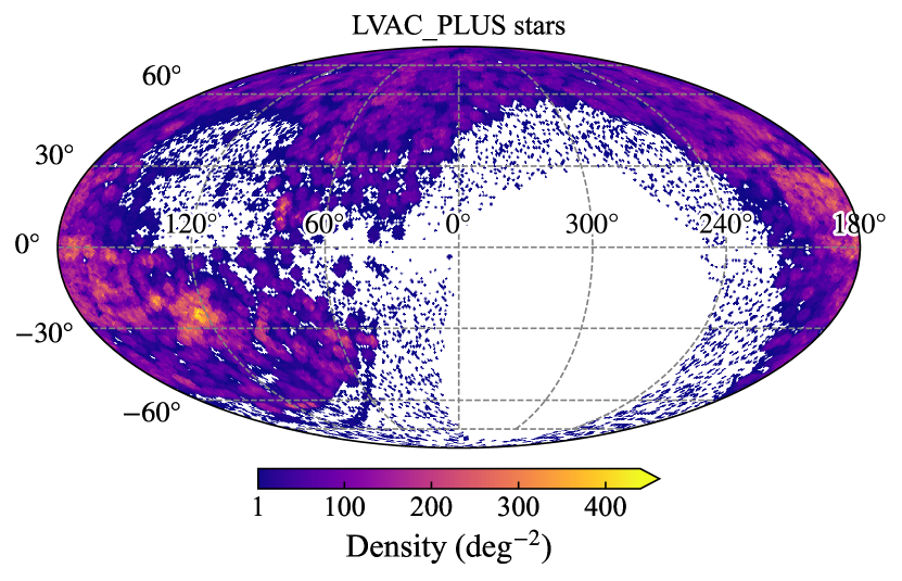
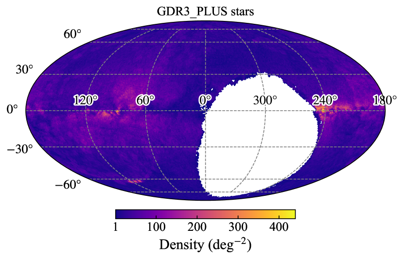
Figure 1: HEALPix (Górski et al., 2005) sky density maps of the ‘LVAC_PLUS’ stellar sample (left) and the ‘GDR3_PLUS’ stellar sample (right). The maps are plotted in Galactic coordinates, with parameter $N_{\mathrm{side}}=64$ and an area of 0.839 $\mathrm{deg}^{2}$ per pixel.

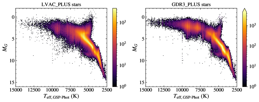
Figure 2: Hertzsprung–Russell (HR) diagrams of the ‘LVAC_PLUS’ stellar sample (left) and the ‘GDR3_PLUS’ stellar sample (right). The effective temperatures are from column teff_gspphot of the Gaia DR3 source table, which are estimated with the General Stellar Parametrizer from Photometry module (GSP-Phot; Andrae et al., 2023; Creevey et al., 2023; Bailer-Jones, 2011). The absolute G-band magnitude is calculated as $M_{G}=G-5\log(1000/\varpi)+5$, where $\varpi$ is the Gaia DR3 parallax in unit of mas. The HR diagrams are color-coded with source number counts in the pixels, the values of which are indicated in the colorbars.

2.2.3 Very low-mass stars, white dwarfs, and carbon stars

Although Gaia DR3 and LAMOST have provided large samples of normal O-to-K-type stars, additional samples of less usual stars are needed to characterize the contaminants in quasar selection. Those unusual stars include M/L/T dwarfs and subdwarfs (also known as very low-mass stars, VLMS), white dwarfs, and carbon stars.

M/L/T dwarfs and subdwarfs are stellar or substellar objects with low masses and low surface temperatures. Because such VLMS emit most of their light in the infrared wavelengths, they can be easily confused with high-redshift or intrinsically red quasars (e.g. Hawley et al., 2002; Richards et al., 2002).

Typical white dwarfs have a blue continuum from optical to near-IR wavelengths, and absorption lines from Hydrogen or Helium, which are very different from typical quasar SEDs. However, central white dwarfs of planetary nebulae (PNe) may show prominent Hydrogen emission lines in addition to the blue continuum, contaminating the quasar candidates (see Figure C1 of Fu et al., 2022, for an example). Some white dwarfs, e.g. the Carbon-rich (DQ) subtype (Pelletier et al., 1986), show wide and deep absorption troughs resulting from Swan bands of the $\rm C_{2}$ molecules, as well as the blue continuum at longer wavelengths. Such white dwarfs are substantial contaminants for broad absorption line (BAL) quasars, and the so-called “3,000 Å break quasars” (Meusinger et al., 2016).

Carbon stars have spectra that are dominated by carbon molecular bands, including the CN, CH, or the Swan bands of C2. The red SEDs of carbon stars are similar to those of high-redshift quasars. Therefore, carbon stars should also be included in the master stellar samples.

We compile a sample of M/L/T dwarfs and subdwarfs, white dwarfs, and carbon stars from a variety of origins, which are listed in Table 1. Cross-matching these additional stars to databases described in Section 2.1 yields a list of stars to be added to the LAMOST and Gaia stellar samples (hereafter “add-on stellar sample”). We build the first master stellar sample LVAC_PLUS by merging the LAMOST stellar sample in Section 2.2.1 and the add-on stellar sample, and build the other master stellar sample GDR3_PLUS by merging the Gaia DR3 stellar sample in Section 2.2.2 and the add-on stellar sample. Figure 1 shows the sky distributions of both LVAC_PLUS and GDR3_PLUS. Both of the two master stellar samples cover a moderately large parameter space of effective temperature and luminosity, as can be seen from their HR diagrams (Figure 2).

Table 1: Additional samples of very low-mass stars, white dwarfs, and carbon stars.

Samples of very low-mass stars (MLT dwarfs & subdwarfs)	Source number	References
Stellar parameter catalog of LAMOST DR6 M dwarf stars	243,231	Li et al. (2021b)
SDSS DR7 spectroscopic M dwarf catalog	70,841	West et al. (2011)
J-PLUS DR2 ultracool dwarf candidates	9,810	Mas-Buitrago et al. (2022)
SVO archive of M dwarfs in VVV	7,925	Cruz et al. (2023)
Ultracool dwarfs in Gaia DR3	7,630	Sarro et al. (2023)
M subdwarfs from LAMOST DR10	3,251	Zhang et al. (2019, 2021)
Photometric brown-dwarf (L/T dwarf) classification	1,361	Skrzypek et al. (2016)
Late-type MLT dwarfs	853	Faherty et al. (2009)
LAMOST DR7 spectroscopic ultracool dwarfs	734	Wang et al. (2022)
L0-T8 dwarfs out to 25 pc	369	Best et al. (2021)
The SVO late-type subdwarf archive	202	Lodieu et al. (2017)
Spectroscopically confirmed L subdwarfs	66	Zhang et al. (2018)
Samples of white dwarfs	Source number	References
The Montreal White Dwarf Database as of 2023/05/18	72,983	Dufour et al. (2017)
SDSS DR7 white dwarf catalog	20,407	Kleinman et al. (2013)
LAMOST DR10 v1.0 white dwarf catalog	17,140	Kong et al. (2018)
White dwarfs within 100 pc with Gaia DR3 and VO	12,718	Jiménez-Esteban et al. (2023)
DB white dwarfs with SDSS and Gaia data	1,915	Genest-Beaulieu & Bergeron (2019)
DB white dwarfs in SDSS DR10 and DR12	1,107	Koester & Kepler (2015)
Samples of carbon stars	Source number	References
General Catalog of Galactic Carbon Stars (3rd edition)	6,891	Alksnis et al. (2001)
Carbon Stars from LAMOST DR4	2,651	Li et al. (2018)
Carbon stars from SDSS	1,211	Green (2013)
Carbon Stars from LAMOST DR2	894	Ji et al. (2016)
High-latitude carbon stars from the Hamburg/ESO survey	403	Christlieb et al. (2001)
Initial catalog of faint high-latitude carbon stars from SDSS	251	Downes et al. (2004)
Carbon stars from the LAMOST pilot survey	183	Si et al. (2015)

2.3 Extragalactic catalogs

2.3.1 SDSS Quasar Catalog: the 16th data release

SDSS (York et al., 2000) has mapped the high Galactic latitude northern sky and obtained imaging as well as spectroscopy data for millions of objects including stars, galaxies, and quasars. The 16th data release of the SDSS Quasar Catalog (SDSS DR16Q; Lyke et al., 2020) contains 750,414 quasars, including 225,082 new quasars appearing in an SDSS data release for the first time, as well as known quasars from SDSS-I/II/III. We cross-match the DR16Q catalog with PS1 and CatWISE2020 both with a radius of $1^{\prime\prime}$.

To ensure data quality, we use the same constraints as in Section 2.1.2 and Section 2.1.3 to retrieve a subset of DR16Q. Because DR16Q contains 421,281 sources whose spectra are not visually inspected, some misidentifications may exist in the sample. We remove 82 false positive sources (non-quasars) mentioned by Flesch (2021). In addition, Wu & Shen (2022) (hereafter WS22) have reported the systemic redshifts ($z_{\mathrm{sys}}$) of DR16Q, which are measured from a comprehensive list of emission lines and are considered superior to the DR16Q redshifts ($z_{\mathrm{DR16Q}}$). We use the two criteria below to select the training/validation sample of 463,497 quasars for the classification model:

1. The spectra should have valid (positive) DR16Q redshifts, and have no known problems in redshift measurements: Z_DR16Q > 0 AND (ZWARNING == 0 OR
ZWARNING == -1), where ‘ZWARNING == -1’ is labeled for visually confirmed quasars prior to DR16Q.

2. The spectra should have valid systemic redshifts ($z_{\mathrm{sys}}$), and are not too noisy or featureless to have line peaks reliably measured (see Section 4.2 of Wu & Shen, 2022): Z_SYS > 0 AND Z_SYS_ERR != -1 AND Z_SYS_ERR != -2.

Nevertheless, for the training/validation sample of the redshift regression models, we apply additional constraints on the uncertainty levels of spectral redshifts. The relative uncertainties in $z_{\mathrm{sys}}$, and the relative differences between $z_{\mathrm{sys}}$ and $z_{\mathrm{DR16Q}}$ are below 0.002:

    Z_SYS_ERR/(1+Z_SYS) < 0.002 AND
    ABS(Z_SYS-Z_DR16Q)/(1+Z_SYS) < 0.002.

The resulted DR16Q subsample for redshift regressions (hereafter the DR16Q redshift subsample) contains 421,959 sources, among which 32,543 sources have Gaia DR3 BP/RP spectra.

2.3.2 SDSS spectroscopically identified galaxies

A sample of galaxies is extracted from SpecPhotoAll table of SDSS Data Release 17 (Abdurro’uf et al., 2022) using the following criteria:

1. The objects are spectroscopically classified as galaxies without broad emission lines detected ($\sigma_{\mathrm{line}}>200\ \mathrm{km\ s^{-1}}$ at the 5-sigma level): CLASS == ‘GALAXY’ AND
SUBCLASS NOT LIKE ‘BROADLINE’.

2. The spectra are primary detections with good observational conditions and high S/N, and no issues are found in fitting the redshifts: SPECPRIMARY == 1 AND PLATEQUALITY == ‘good’ AND
SN_MEDIAN_ALL > 5 AND ZWARNING == 0.

We cross-match the galaxy sample with PS1 and CatWISE2020 with a radius of $1^{\prime\prime}$. We also apply quality constraints in Section 2.1.2 and Section 2.1.3 to select a galaxy subset with good photometry for later use. The resulted subset of galaxies has 485,429 sources.

2.3.3 The Million Quasars (Milliquas) Catalog

The Million Quasars Catalog (Milliquas v8; Flesch, 2023) is a compilation of quasars and quasar candidates from the literature up to 30 June 2023. Milliquas includes 907,144 type 1 QSOs and AGN, 66,026 high-confidence (pQSO=99%) photometric quasar candidates, 2,814 BL Lac objects, and 45,816 type 2 objects.

We use the Milliquas catalog to supplement the training/validation samples at $z<0.5$ or $z>2.5$ for both photometric and BP/RP spectral redshift estimation (Section 6), because the DR16Q redshift subsample (Section 2.3.1) lacks quasars at these low and high redshift ends.

For the photometric redshift regression model, we select 41,410 quasars and type-1 AGNs (labeled as ‘Q’ or ‘A’ in the ‘TYPE’ column of Milliquas) at $0<z<0.5$ or $z>2.5$ from Milliquas using the same constraints of Gaia  PS1, and CatWISE data as in Section 2.1. The 41,410 Milliquas quasars are combined with the DR16Q redshift subsample to form the training/validation sample of 453,977 unique sources.

For the BP/RP spectral redshift model, we select 10,033 quasars and type-1 AGNs that have BP/RP spectra at $z<0.5$ or $z>2.5$ from Milliquas. The union of this Milliquas subsample with 10,033 sources and the DR16Q redshift subsample with BP/RP spectra has 37,992 sources, which serves as the parent sample of training/validation in Section 6.2.

3 Feature selection and characterization

As has been proposed and tested by many previous studies (e.g. Khramtsov et al., 2019; Jin et al., 2019), color indices (or flux ratios) constructed from multiband photometric catalogs are effective features for classifying and predicting photometric redshifts of quasars. In addition, morphological features such as the difference of the PSF and aperture/Kron magnitude have been used either in the machine learning selection of quasars (e.g. Fu et al., 2021), or in the removal of extended sources (galaxies) beforehand (e.g. Richards et al., 2009; Wenzl et al., 2021).

Another useful indicator of source extent is the BP and RP excess factor (phot_bp_rp_excess_factor) from Gaia, which is defined as the ratio of the sum of the integrated BP and RP fluxes to the flux in the G band: $C=(I_{\mathrm{BP}}+I_{\mathrm{RP}})/I_{G}$. Because the detection windows (apertures) of BP and RP bands are wider than that of the G band, extended sources tend to have larger flux excess factors than the point sources do (see e.g. Liu et al., 2020). However, a strong dependence on the $G_{\mathrm{BP}}-G_{\mathrm{RP}}$ color is observed in the flux excess factor $C$, which increases with redder colors and flattens out at the blue end (Riello et al., 2021). To better constrain the actual source extent from the flux excess, we adopt the corrected BP-RP flux excess factor $C^{*}$ following the recipe of Riello et al. (2021) , which removes the dependence of $C$ on $G_{\mathrm{BP}}-G_{\mathrm{RP}}$ by fitting and subtracting three polynominals.

Using PSF magnitudes ($grizy_{\mathrm{P1}}$, hereafter $grizy$ for simplicity) from PS1, profile-fit photometry including motion from CatWISE2020 (w1mpro_pm and w2mpro_pm, hereafter W1 and W2), and broadband photometry from Gaia DR3, we computed a list of features for source classification: $g-r$, $r-i$, $i-z$, $z-y$, $g-\mathrm{W1}$, $r-\mathrm{W1}$, $i-\mathrm{W1}$, $z-\mathrm{W1}$, $y-\mathrm{W1}$, $\mathrm{W1}-\mathrm{W2}$, $G_{\mathrm{BP}}-G_{\mathrm{RP}}$, $G_{\mathrm{BP}}-G$, $G-G_{\mathrm{RP}}$, and $C^{*}$.

A few color features of quasars, galaxies, and stars are shown as color-color diagrams in Figure 3. Quasars and galaxies are typically clustered around regions with the highest densities in the two-dimensional color spaces, which results in smooth contours in the diagrams. On the contrary, stars are largely distributed on narrow stripes in color-color diagrams, which are referred to as stellar loci.

In general, quasars are bluer than galaxies and stars in optical bands because quasars have power-law continua and broad emission lines in the rest-frame UV to optical wavelengths. Nevertheless, the quasar loci overlap heavily with those of galaxies and stars in the color-color diagrams built from the four PS1 colors ($g-r$, $r-i$, $i-z$, and $z-y$).

At longer wavelengths, quasars show larger infrared excesses in comparison to stars due to the power-law emission from the accretion disk and the existence of cold to hot dust around quasars. Quasars can therefore be separated from most stars in color-color diagrams that involve near-infrared and mid-infrared bands ($y$, W1, and W2). However, the infrared selections of quasars are still contaminated by red stars including M/L/T dwarfs or subdwarfs, AGB stars, and young stellar objects (YSOs).

Figure 4 shows the corrected flux excess factor $C^{*}$ versus $G_{\mathrm{BP}}-G_{\mathrm{RP}}$ for quasars, galaxies, and stars. The $C^{*}$ factors of stars remain nearly zero despite the change in $G_{\mathrm{BP}}-G_{\mathrm{RP}}$ colors, as defined in Riello et al. (2021). The $C^{*}$ factors of quasars are also close to zero, although they have a larger scatter than those of stars. The $C^{*}$ factors of galaxies are much larger than those of stars and quasars, making $C^{*}$ a good indicator of the extent of the source.

Figure 3: Color-color diagrams of 200,000 quasars (blue contours), 200,000 galaxies (green contours), and 400,000 stars (red-shaded density plots) using photometric data from PS1, CatWISE and Gaia DR3. The quasar and galaxy samples are random subsets of the quasar and galaxy samples described in Section 2.3.1 and 2.3.2. The star sample is randomly selected from the union of LVAC_PLUS and GDR3_PLUS. The density plots of stars are color-coded with density, with higher density being darker, and lower density being lighter. All magnitudes are in the AB system.

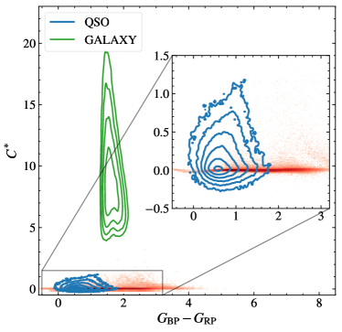
Figure 4: Corrected flux excess factor $C^{*}$ versus $G_{\mathrm{BP}}-G_{\mathrm{RP}}$ color for stars (red-shaded density plots), quasars (blue contours), and galaxies (green contours). An inset of zoom-in plot for stars and quasars is displayed on the upper-right corner.

4 Source classification with the XGBoost algorithm

We use XGBoost (Chen & Guestrin, 2016), a gradient boosting decision tree algorithm to train the machine learning classification model, and reclassify the input Gaia DR3 quasar candidates as quasars, stars, and galaxies. By keeping the extragalactic samples fixed and alternating between two master samples of stars (LVAC_PLUS and GDR3_PLUS), we compose two sets of training/validation data using the 14 photometric features selected in Section 3. Such configuration is helpful for obtaining two classification models that can be later combined. We use “CLF_LVAC” to denote the classifier trained with LAMOST stars, and “CLF_GDR3” to denote the classifier trained with Gaia stars.

In order to obtain the optimal models, we use optuna (Akiba et al., 2019), a hyperparameter optimization framework to tune the learning hyperparameters. The multi-class log loss $L_{\log}(Y,P)$ (also known as logistic regression loss, or cross-entropy loss) is used as the objective function to be minimized during model training and hyperparameter optimization. For a classification task with $K$ classes and $N$ samples, let the true label of sample $i$ be encoded as a binary indicator $y_{i,k}\in\{0,1\}$, then $y_{i,k}=1$ when sample $i$ has label $k$. A probability estimate is defined as $p_{i,k}=\operatorname{Pr}(y_{i,k}=1)$. Let $P$ be the matrix of probability estimates and $Y$ be the matrix of encoded labels, then the log loss of the whole set is the negative log-likelihood of the classifier given the true labels:

$$\begin{split}L_{\log}(Y,P)&=-\ln\operatorname{Pr}(Y|P)\\ &=-\frac{1}{N}\sum_{i=0}^{N-1}\sum_{k=0}^{K-1}y_{i,k}\ln p_{i,k}.\end{split}$$ (1)

The log loss is a statistical measure of the distance between the empirical distribution of the data and the predicted distribution.

Another few metrics are used to evaluate the model performance: balanced accuracy, precision, recall, $F_{1}$, and Matthews correlation coefficient (MCC). For binary classification problems, with true positive denoted as TP, true negative as TN, false positive as FP, and false negative as FN, the five metrics are defined as:

$$\rm balanced\ accuracy=\frac{1}{2}\left(\frac{TP}{TP+FN}+\frac{TN}{TN+FP}\right)$$ (2)

$$\rm precision=\frac{TP}{TP+FP}$$ (3)

$$\rm recall=\frac{TP}{TP+FN}$$ (4)

$$F_{1}=\rm 2\times\frac{precision\times recall}{precision+recall}$$ (5)

$$\rm MCC=\frac{TP\times TN-FP\times FN}{\sqrt{(TP+FP)(TP+FN)(TN+FP)(TN+FN)}}.$$ (6)

In the case of a multiclass problem, the classification task is treated as a collection of binary classification problems, one for each class. The five metrics above can be calculated for each binary classification problem (each class). The metrics of the multiclass problem is the average metrics of all classes. We adopt functions balanced_accuracy_score, precision_score, recall_score, f1_score, and matthews_corrcoef of the sklearn.metrics module of scikit-learn (Pedregosa et al., 2011) to calculate the metrics for the three-class classification problem in this work. When calculating precision, recall, and $F_{1}$, the ‘weighted’ strategy is used, in which the score of each class is weighted by its fraction in the true data sample.

We first apply five-fold cross validations with optuna (Akiba et al., 2019) to find the optimal setting of hyperparameters that minimizes the log loss among 500 trials. Then we randomly split the whole input data into training set and validation set according to a $4:1$ ratio and calculate scores of the five metrics with the validation set. This $4:1$ split ratio is consistent with that of the five-fold cross validations. The large sample size of input data also ensures both training and validation sets have enough samples.

Some fixed parameters in our programs are: objective=multi:softprob; booster=gbtree; tree_method=hist. For hyperparameters that are tuned, the default values, optimal values found by the cross validations, and corresponding metric scores of these parameters are listed in Table 2. In the tuning process, the number of boosting rounds (num_boost_round, a.k.a. n_estimators in scikit-learn API of XGBoost) is fixed to 100 and eta (a.k.a. learning_rate) is fixed to 0.1. In the training process, we need to lower the learning rate eta and increase the num_boost_round to reduce the generalization error. Both CLF_LVAC and CLF_GDR3 are trained using $\mathtt{eta}=0.01$, $\mathtt{num\_boost\_round}=5000$ with other optimal parameters obtained with optuna.

Table 2: Default and optimal hyperparameter settings for CLF_LVAC and CLF_GDR3 ($\mathtt{eta}=0.1$, $\mathtt{num\_boost\_round}=100$).

Hyperparameter	CLF_LVAC		CLF_GDR3
	Default	Optimal	Default	Optimal
lambda	1	1.18	1	1.32
alpha	0	1.61	0	0.33
max_depth	6	9	6	9
gamma	0	0.71	0	0.18
grow_policy	depthwise	lossguide	depthwise	lossguide
min_child_weight	1	3	1	4
subsample	1	0.87	1	0.70
colsample_bytree	1	0.61	1	0.74
max_delta_step	0	5	0	8
Balanced accuracy	0.9972	0.9977	0.9973	0.9979
Precision (weighted)	0.9981	0.9985	0.9982	0.9985
Recall (weighted)	0.9981	0.9985	0.9982	0.9985
$F_{1}$ (weighted)	0.9981	0.9985	0.9982	0.9985
MCC	0.9967	0.9973	0.9968	0.9975

With CLF_LVAC and CLF_GDR3, we predict the probabilities of the input sources for being quasars, stars, and galaxies. We average the predictions of the two classifiers and obtain the mean probabilities ($p_{\mathrm{QSO\_mean}}$, $p_{\mathrm{star\_mean}}$, and $p_{\mathrm{galaxy\_mean}}$). Sources with $p_{\mathrm{QSO\_mean}}>0.95$ are kept as reliable quasar candidates.

5 Additional filtering with Gaia proper motions

In order to remove stellar contaminants such as white dwarfs, M/L/T dwarfs, YSOs, and AGB stars from quasar candidates, we apply an additional cut based on Gaia proper motion, because the proper motion distribution of quasars is different from that of Milky Way stars. Although quasars should have negligible transverse motions, non-zero proper motions of them are measured by Gaia due to various effects, such as photocenter variability of quasars (see Bachchan et al., 2016, and references therein), and double/multiple sources (Makarov & Secrest, 2022). In addition, proper motions with large uncertainties are not reliable. Therefore we need a probabilistic cut instead of a cut on the total proper motion. In Fu et al. (2021), we defined the probability density of zero proper motion ($f_{\mathrm{PM0}}$) of a source, based on the bivariate normal distribution of proper motion measurements of the source as:

$$f_{\mathrm{PM0}}=\frac{1}{2\pi\sigma_{x}\sigma_{y}\sqrt{1-\rho^{2}}}\times\\ \mathrm{exp}\left\{-\frac{1}{2(1-\rho^{2})}\left[\left(\frac{x}{\sigma_{x}}\right)^{2}-\frac{2\rho xy}{\sigma_{x}\sigma_{y}}+\left(\frac{y}{\sigma_{y}}\right)^{2}\right]\right\},$$ (7)

where $x=\mathrm{pmra}$, $y=\mathrm{pmdec}$, $\rho=\mathrm{pmra\_pmdec\_corr}$ (correlation coefficient between pmra and pmdec), $\sigma_{x}$ and $\sigma_{y}$ are the proper motion uncertainties. Under the same uncertainty level, sources with smaller proper motions will have higher $f_{\mathrm{PM0}}$ by definition.

We take the logarithm of $f_{\mathrm{PM0}}$ for better comparison between samples. Figure 5 shows distributions of $\log(f_{\mathrm{PM0}})$ of stars, galaxies and quasars used in this study. We choose a $\log(f_{\mathrm{PM0}})\geq-4$ cut that excludes more than 99.9% of both LVAC_PLUS and GDR3_PLUS stars, while retaining more than 99.8% of the quasars. Nevertheless, faint stars can be major contaminants even with such strict cut on $\log(f_{\mathrm{PM0}})$.

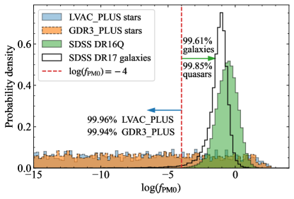
Figure 5: Histograms of $\log(f_{\mathrm{PM0}})$ of the master stellar samples ‘LVAC_PLUS’ (blue) and ‘GDR3_PLUS’ (yellow), quasars from SDSS DR16Q (green), and galaxies from SDSS DR17 (white). Because $f_{\mathrm{PM0}}$ is the probability density which can be greater than 1 (the integral of the probability density function over the entire space is equal to 1), $\log(f_{\mathrm{PM0}})$ can have positive values.

6 Photometric and spectroscopic redshifts with machine learning

Accurate redshift estimation is essential to both cosmology and follow-up studies with the quasar candidates. For all sources of our quasar candidate sample, photometric redshifts are derived from photometric data from Gaia DR3, PS1, and CatWISE using an ensemble machine learning regression model. For a subset of 89,100 quasar candidates with BP/RP spectra, spectroscopic redshifts are also measured using a convolutional neural network (CNN) regression model.

For both regression models, we adopt the root mean square error (RMSE), the normalized median absolute deviation of errors ($\sigma_{\mathrm{NMAD}}$), and the catastrophic outlier fraction ($f_{\mathrm{c}}$) as evaluation metrics for the estimation of the redshift in the training/validation sets. These metrics are defined as follows:

$$\mathrm{RMSE}=\sqrt{{\frac{1}{n}}\sum_{i=1}^{n}\left(z_{i}-{\hat{z_{i}}}\right)^{2}}$$ (8)

$$\sigma_{\mathrm{NMAD}}=1.48\times\mathrm{median}\left(\left|\frac{\Delta z-\mathrm{median}(\Delta z)}{1+z}\right|\right)$$ (9)

$$f_{\mathrm{c}}=\frac{1}{n}\times\mathrm{count}\left(\left|\frac{\Delta z}{1+z}\right|>0.15\right),$$ (10)

where $z$ is the true redshift, $\hat{z}$ is the predicted redshift, $\Delta z=z-\hat{z}$, and $n$ is the total number of sources. The RMSE is widely used in regression analysis to quantify the difference between the true and predicted values. The $\sigma_{\mathrm{NMAD}}$ measures the statistical dispersion of the normalized errors $\Delta z^{\prime}=\Delta z/(1+z)$. When $\Delta z^{\prime}$ follows a Gaussian distribution, this $\sigma_{\mathrm{NMAD}}$ is equivalent to the standard deviation of $\Delta z^{\prime}$. In real-world cases, $\sigma_{\mathrm{NMAD}}$ is less sensitive to outliers than the original definition of standard deviation (Ilbert et al., 2006; Brammer et al., 2008). The $f_{\mathrm{c}}$ represents the percentage of objects for which the redshift estimate deviates significantly from the true redshift.

In addition to the evaluation metrics, a loss function (or objective function) must be defined when training the redshift regression models. By minimizing the value of the loss function, the regression model learns the best fit to the training data. When training photometric redshift regression models, we choose the loss functions from the built-in functions provided by the software packages. Because our BP/RP spectroscopic redshift regression model is more flexible than the photometric ones, we adopt a custom loss function, the mean normalized square error (MNSE), which is defined as:

$$\mathrm{MNSE}={\frac{1}{n}}\sum_{i=1}^{n}\left(\frac{z_{i}-{\hat{z_{i}}}}{1+z_{i}}\right)^{2}.$$ (11)

While the definition of MNSE is similar to that of the commonly used mean square error (MSE; that is, the square of the RMSE), MNSE makes the squared errors comparable across different redshifts by dividing each error $z_{i}-{\hat{z_{i}}}$ by a factor of $1+z_{i}$. Minimizing MNSE is also very helpful to build an optimal model with low $\sigma_{\mathrm{NMAD}}$ and $f_{c}$ values.

6.1 An ensemble photometric redshift model with XGBoost, TabNet, and FT-Transformer

The photo-z estimation problem can be well described as a regression problem on tabular data in machine learning. While traditionally tree ensemble models (e.g. XGBoost) are widely applied to such problems, some deep learning models have also been shown to be highly efficient in regression problems of tabular data, including TabNet (Arik & Pfister, 2021) and FT-Transformer (Gorishniy et al., 2021). Here, we adopt XGBoost, TabNet and FT-Transformer to train three separate machine learning models to estimate redshifts from multiband photometry. We optimize the models independently and combine their results. By averaging the predictions of the three models, we obtain the ensemble photometric redshift model, which improves the predictive performance of a single model (Sagi & Rokach, 2018).

To mitigate the influence of undersampling of quasars at both low ($z<0.5$) and high ($z>2.5$) redshifts in SDSS DR16Q (subset for redshift regression described in Section 2.3.1), we add 41,410 additional quasars and type-1 AGNs at $z<0.5$ or $z>2.5$ from the Milliquas v8 catalog (Flesch, 2023) to build the training/validation sample of 453,977 unique quasars. We randomly split the sample with a ratio of $4:1$ into the training set and validation set. The training and validation sets and our application set (the CatNorth sample) are all dereddened with the two-dimensional dust map from Planck Collaboration et al. (2016) and the extinction law from Wang & Chen (2019).

The redshift estimates of the GDR3 QSO candidates (redshift_qsoc, hereafter $z_{\mathrm{Gaia}}$) are determined using a chi-square approach, whereby the BP and RP spectra are compared to a composite quasar spectrum at various trial redshifts in the range of $0\lesssim z\lesssim 6$ (Gaia Collaboration et al., 2023b; Delchambre et al., 2023). The composite quasar spectrum is built upon a semi-empirical library of quasars from the SDSS DR12Q sample (Pâris et al., 2017). Although $z_{\mathrm{Gaia}}$ can have higher precision than photometric redshifts, $z_{\mathrm{Gaia}}$ has a high catastrophic outlier fraction due to emission line misidentification (aliasing) in the chi-square fitting process. Storey-Fisher et al. (2023) demonstrated that the outlier fraction of redshifts can be significantly reduced by using both $z_{\mathrm{Gaia}}$ and photometric features in the machine learning process.

Similar to the redshift estimation approach of Storey-Fisher et al. (2023), we combine redshift information from the GDR3 QSO candidate catalog and a set of photometric features to train the photometric redshift models. Instead of using $z_{\mathrm{Gaia}}$ as a feature directly, we build two new features $\log(1+z_{\mathrm{low}})$ and $\log(1+z_{\mathrm{up}})$, where $z_{\mathrm{low}}$ (redshift_qsoc_lower) and $z_{\mathrm{up}}$ (redshift_qsoc_upper) are the lower and upper confidence intervals of $z_{\mathrm{Gaia}}$ taken at 0.15866 and 0.84134 quantiles, respectively. The logarithmic transformation on $1+z$ compresses the high redshift range with fewer training samples and large uncertainties, and produces a nearly Gaussian distribution of the new feature (see also Section 5.2.3 of Delchambre et al., 2023, on the normality of $\log(1+z)$).

A total of 15 features are chosen for the regression model: $g-r$, $r-i$, $i-z$, $z-y$, $g-\mathrm{W1}$, $r-\mathrm{W1}$, $i-\mathrm{W1}$, $z-\mathrm{W1}$, $y-\mathrm{W1}$, $\mathrm{W1}-\mathrm{W2}$, $G_{\mathrm{BP}}-G_{\mathrm{RP}}$, $G_{\mathrm{BP}}-G$, $G-G_{\mathrm{RP}}$, $\log(1+z_{\mathrm{low}})$, and $\log(1+z_{\mathrm{up}})$. Some features may contain missing values in the training/validation and final application (CatNorth) samples. We imput the missing values with the mean values of the training sample to ensure valid redshift estimation for all targets.

We choose the default RMSE as the loss function of the XGBoost model, and the smooth L1 loss as the loss function of both the TabNet and the FT-Transformer models. Using the same notation above, the smooth L1 loss of the $i$-th instance of the data is:

$$l_{i}=\begin{cases}0.5(z_{i}-\hat{z}_{i})^{2}&\text{if }|z_{i}-\hat{z}_{i}|<1\\ |z_{i}-\hat{z}_{i}|-0.5&\text{otherwise},\end{cases}$$ (12)

and the overall smooth L1 loss is then the mean value:

$$L_{1}={\frac{1}{n}}\sum_{i=1}^{n}l_{i}.$$ (13)

The smooth L1 loss is less sensitive to the outliers in the data in comparison to MSE (Girshick, 2015).

Each model is trained with its optimal hyperparameters found by optuna. The scores of the three regression models and the ensemble model on a validation set of 82,415 sources are listed in Table 3. Among the three base models, TabNet has the lowest RMSE (0.2685), $\sigma_{\mathrm{NMAD}}$ (0.0303) and $f_{\mathrm{c}}$ (9.04%). Averaging the three base models produces an ensemble model with even lower RMSE (0.2618) and $\sigma_{\mathrm{NMAD}}$ (0.0294), and a moderately low $f_{\mathrm{c}}$ (9.16%). Because ensemble models are less sensitive to over-fitting than other models, we expect the ensemble model to be more robust than the individual base models.

6.2 BP/RP spectroscopic redshift model with the Convolutional Neural Network

The Gaia DR3 BP/RP spectra provide valuable spectral information, offering a unique opportunity to infer the redshifts of distant quasars. Here, we adopt a CNN-based regression model (hereafter RegNet) to extract redshifts of quasars encoded in the BP/RP spectra. The parent sample of 37,992 quasars that have BP/RP spectra is described in Section 2.3.3. A $4:1$ ratio is used to randomly divide the BP/RP spectral sample into training and validation sets. For both training/validation sample and the final application sample, we obtain the original continuous BP/RP spectra (coefficients) with the astroquery.gaia module. We then use the GaiaXPy package (Ruz-Mieres, 2023) to sample the spectra to $\mathrm{[4000\AA,10000\AA)}$ with a 20Å interval, and calibrate the spectra to absolute fluxes.

The RegNet architecture consists of four convolutional layers followed by two fully connected linear layers, culminating in a 1D output for redshift estimation. Each input spectrum contains 300 data points (neurons) and is scaled to $[0,1]$ with its minimum and maximum values. Each convolutional layer has 8 channels and a kernel size of 3, the output of which goes through a ReLU activation function and a MaxPool function with a kernel size of 2. The first fully connected layer (FC1) connects all neurons from the last convolutional layer (Conv4) to 128 neurons and applies a ReLU activation function to the output. The last fully connected layer (FC2) connects the 128 neurons to a single neuron, and uses a SoftPlus activation function to ensure the final output is always positive. A schematic diagram of the RegNet architecture is shown in Figure 6.

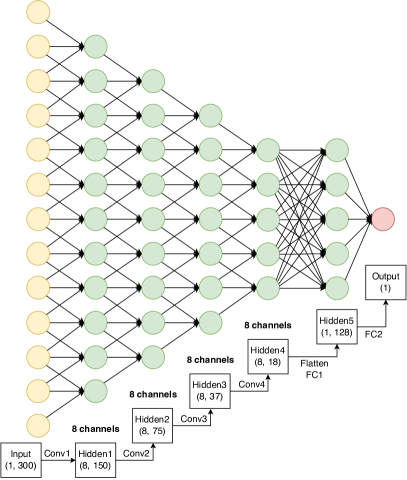
Figure 6: Schematic diagram of the CNN-based RegNet architecture, which is designed to extract redshifts from Gaia DR3 BP/RP spectra. This diagram shows the process of a single spectrum with 300 points passing through the network and yielding the redshift value. For simplicity, only a small fraction of the input and hidden neurons are plotted.

The RegNet model is trained in shuffled batches, each of which contains 1024 spectra. With the default parameters of the Adam optimizer (torch.optim.Adam), we train the RegNet model for 1,000 epochs. The MNSE losses for all epochs of training and validation data are shown in Figure 7. The optimal model is from the epoch with the lowest validation loss, that is, the 1,000th epoch with $\mathrm{MNSE_{val}}=0.00403$. On the validation set of 7,599 quasars at $0<z\lesssim 4.0$, the RegNet model achieves $\mathrm{RMSE}=0.1427$, $\sigma_{\mathrm{NMAD}}=0.0304$, and $f_{\mathrm{c}}=2.46\%$. The uncertainty $\sigma_{\mathrm{NMAD}}=0.0304$ of our model is close to that of Cristiani et al. (2023), which is 0.02 and was measured with 934 quasars at $2.5\lesssim z\lesssim 4.0$.

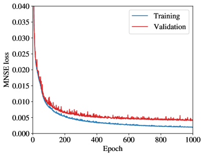
Figure 7: The MNSE losses in 1,000 epochs of our RegNet model on the training sample (blue curve) and validation sample (red curve). As the model is trained iteratively, the training loss steadily decreases, signifying the network’s ability to fit the training set. Meanwhile, the validation loss from an independent validation set demonstrates the generalization performance of the model.

Table 3: Scores of all photometric redshift regression models (XGBoost, TabNet, FT-Transformer, and the ensemble model), and the spectroscopic redshift regression model (RegNet) on the validation sets.

	Photo-$z$ models				Gaia BP/RP spec-$z$ model
Model	XGBoost	TabNet	FT-Transformer	Ensemble	RegNet
	RMSE	Smooth L1	Smooth L1		MNSE
RMSE	0.2734	0.2685	0.2723	0.2618	0.1427
$\sigma_{\mathrm{NMAD}}$	0.0351	0.0303	0.0307	0.0294	0.0304
$f_{\mathrm{c}}$	10.65%	9.04%	9.21%	9.16%	2.46%

6.3 Performance of the photometric and spectroscopic redshifts

The precision of the RegNet spectroscopic redshift model is about twice those of the photometric redshift models as measured with RMSE (see Table 3). The $\sigma_{\mathrm{NMAD}}$ of RegNet and the photometric redshift models are close because the Gaia redshift information is used in the photometric redshift models. The outlier fraction of RegNet is about only 1/4 of those of the photo-$z$ models. Such good performance of RegNet indicates the feasibility of identifying quasars and studying their properties with the Gaia BP/RP low-res spectra.

With the ensemble photometric redshift regression model and the RegNet model, we derive photometric redshifts for all quasar candidates in our work, and spectroscopic redshifts for a subset of 89,100 sources with Gaia DR3 BP/RP spectra. In Figure 8, we show the performance of the redshift regression models on the validation sets, and the comparisons between our redshift estimates and those from the GDR3 QSO candidate catalog and the Quaia catalog.

The ensemble photometric redshift $z_{\mathrm{ph}}$ is highly consistent with the RegNet spectroscopic redshift $z_{\mathrm{xp\_nn}}$ (Figure 8 (c)), which proves the reliability of both redshift estimates because $z_{\mathrm{ph}}$ and $z_{\mathrm{xp\_nn}}$ are obtained with entirely different methods. The original Gaia DR3 redshift $z_{\mathrm{Gaia}}$ presents large deviations from $z_{\mathrm{SDSS}}$, and $z_{\mathrm{ph}}$ and $z_{\mathrm{xp\_nn}}$ in this work (Figure 8 (d, e & f)), which is mainly because only the Gaia data were used to derive $z_{\mathrm{Gaia}}$ (Gaia Collaboration et al., 2023b). The distribution of the outliers on $z_{\mathrm{ph}}-z_{\mathrm{Gaia}}$ plot (Figure 8 (e)) is similar to that of the $z_{\mathrm{SDSS}}-z_{\mathrm{Gaia}}$ plot (Figure 8 (d)), which indicates that the line misidentification in the GDR3 QSO candidate catalog is systematic, and that the CatNorth $z_{\mathrm{ph}}$ is consistent with $z_{\mathrm{SDSS}}$.

A much lower outlier fraction is seen in $z_{\mathrm{xp\_nn}}-z_{\mathrm{Gaia}}$ plot (Figure 8 (f)) in comparison to $z_{\mathrm{SDSS}}-z_{\mathrm{Gaia}}$ and $z_{\mathrm{ph}}-z_{\mathrm{Gaia}}$, because only a subsample with Gaia DR3 BP/RP spectra has available $z_{\mathrm{xp\_nn}}$. Nevertheless, the outliers around ($z_{\mathrm{Gaia}}\approx 0.5,z_{\mathrm{xp\_nn}}\approx 1.2$), ($z_{\mathrm{Gaia}}\approx 2.5,z_{\mathrm{xp\_nn}}\approx 1.3$), and ($z_{\mathrm{Gaia}}\approx 3.5,z_{\mathrm{xp\_nn}}\approx 1.0$) on $z_{\mathrm{xp\_nn}}-z_{\mathrm{Gaia}}$ plot match the high-density outlier regions in $z_{\mathrm{SDSS}}-z_{\mathrm{Gaia}}$ and $z_{\mathrm{ph}}-z_{\mathrm{Gaia}}$. Such outlier patterns also indicate that $z_{\mathrm{xp\_nn}}$ is more robust than $z_{\mathrm{Gaia}}$.

For sources with correct emission line identifications, $z_{\mathrm{Gaia}}$ has high precision because of the direct use of BP/RP spectra in the chi-square fitting process. Therefore $z_{\mathrm{Gaia}}$ has a lower $\sigma_{\mathrm{NMAD}}$ (0.0073) than CatNorth $z_{\mathrm{ph}}$ (0.0294) despite the high outlier fraction $f_{\mathrm{c}}=26.6\%$ of the former. The Quaia redshift also shows a low $\sigma_{\mathrm{NMAD}}$ (0.0078) because $z_{\mathrm{Quaia}}$ is replaced with $z_{\mathrm{Gaia}}$ when the two estimates are close to each other ($|\Delta z/(1+z)|<0.05$; see Storey-Fisher et al., 2023).

To evaluate the quality of redshift estimates of the GDR3 QSO candidates, De Angeli et al. (2023) defined the logarithmic redshift error between the redshift estimate $z_{\mathrm{pred}}$ and the literature redshift $z_{\mathrm{true}}$ as

$$\Delta Z=\log(1+z_{\mathrm{pred}})-\log(1+z_{\mathrm{true}}).$$ (14)

If an emission line with a rest-frame wavelength of $\lambda_{\mathrm{true}}$ is misidentified as another one with a rest-frame wavelength of $\lambda_{\mathrm{false}}$, the logarithmic redshift error is $\Delta Z=\log\lambda_{\mathrm{true}}-\log\lambda_{\mathrm{false}}$. Therefore the most frequent mismatches between emission lines can be identified through the distribution of $\Delta Z$.

We compare the distributions of $\Delta Z$ of $z_{\mathrm{Gaia}}$, $z_{\mathrm{Quaia}}$, and CatNorth $z_{\mathrm{ph}}$ for 286,107 SDSS DR16Q sources in common in Figure 9. While the Quaia redshift $z_{\mathrm{Quaia}}$ shows large improvement over $z_{\mathrm{Gaia}}$, $z_{\mathrm{Quaia}}$ inherits some line misidentifications from $z_{\mathrm{Gaia}}$. For example, the C iv emission line is often misidentified as Ly$\alpha$, which produces a peak at $\Delta Z=0.11$ in Figure 9, as well as the high-density region of $2.2\lesssim z_{\mathrm{Quaia}}\lesssim 3.2$ and $1.5\lesssim z_{\mathrm{SDSS}}\lesssim 2.2$ of Figure 8 (g). In less frequent cases, the C iv emission line is misidentified as C iii] ($\Delta Z=-0.09$), or the C iii] emission line is misidentified as Mg ii ($\Delta Z=-0.17$) or Ly$\alpha$ ($\Delta Z=0.2$). The logarithmic redshift error of CatNorth $z_{\mathrm{ph}}$ has a much smoother distribution and overall deviates less from zero than those of $z_{\mathrm{Gaia}}$ and $z_{\mathrm{Quaia}}$, showing the robustness of the $z_{\mathrm{ph}}$ estimates.

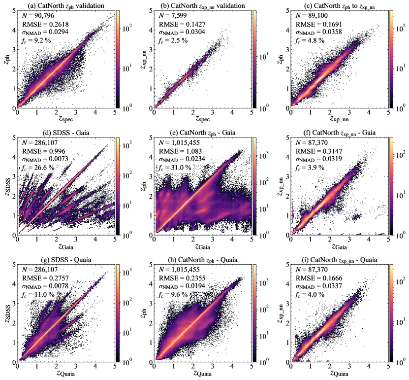
Figure 8: Top row: ensemble photometric redshift ($z_{\mathrm{ph}}$) against SDSS/Milliquas spectral redshift of the validation set with 90,796 quasars (a), RegNet redshift ($z_{\mathrm{xp\_nn}}$) against SDSS/Milliquas spectral redshift of the validation set with 7,599 quasars (b), and $z_{\mathrm{ph}}$ versus $z_{\mathrm{xp\_nn}}$ (c). Middle row: comparisons of redshift values between SDSS and Gaia (d), CatNorth $z_{\mathrm{ph}}$ and Gaia (e), and CatNorth $z_{\mathrm{xp\_nn}}$ and Gaia (f). Bottom row: comparisons of redshift values between SDSS and Quaia (g), CatNorth $z_{\mathrm{ph}}$ and Quaia (h), and CatNorth $z_{\mathrm{xp\_nn}}$ and Quaia (i). The plots are color-coded with two-dimensional densities (number counts in the pixels) of the samples, the values of which are indicated in the colorbars.

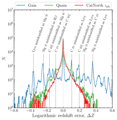
Figure 9: Histograms of the logarithmic redshift errors, $\Delta Z=\log(1+z)-\log(1+z_{\mathrm{SDSS}})$ of $z_{\mathrm{Gaia}}$ (blue), $z_{\mathrm{Quaia}}$ (green), and CatNorth $z_{\mathrm{ph}}$ (red), for 286,107 sources contained in the SDSS DR16Q catalog. A bin width of 0.0026 is used for all curves. Several prominent peaks due to emission line misidentifications are indicated with vertical dashed lines and texts.

For quasar candidates with Gaia DR3 BP/RP spectra, the redshift estimates can also be validated by visual inspections of the spectra. The Gaia DR3 BP/RP spectra that are calibrated with GaiaXPy of four CatNorth quasars are shown in Figure 10 along with the template quasar spectrum from Vanden Berk et al. (2001). The template quasar spectrum matches well to the BP/RP spectra after being shifted to $z_{\mathrm{xp\_nn}}$. However, because the spectral resolution of the BP/RP spectra is very low ($R\sim 50$), and the uncertainties in the sampled spectra (e.g. calibrated spectra in this work) are not well quantified (see De Angeli et al., 2023, for detailed discussions), the accuracy of $z_{\mathrm{xp\_nn}}$ is still lower than that of the SDSS spectral redshifts.

Figure 10: The Gaia DR3 BP/RP spectra that are calibrated with GaiaXPy of four CatNorth quasars (in black). For each quasar, a template quasar spectrum of Vanden Berk et al. (2001) is shown as a blue line in addition to the BP/RP spectrum. The template spectrum is shifted to the same redshift of $z_{\mathrm{xp\_nn}}$, and scaled to a similar flux level of the BP/RP spectrum. Some major emission lines of the template spectrum are marked with red dashed lines.

7 Results: The CatNorth Quasar Candidate Catalog

7.1 Description of the CatNorth quasar candidate catalog

We compile the CatNorth quasar candidate catalog based on the sample selected from Sections 4 and 5, with derived quantities from this work, and some selected columns from PS1 DR1, CatWISE2020, and Gaia DR3. The description for the CatNorth quasar candidate catalog is displayed in Table 4.

Table 4: Format of the CatNorth quasar candidate catalog.

Column	Name	Type	Unit	Description
1	source_id	long	…	Gaia DR3 unique source identifier
2	ra	double	deg	Gaia DR3 right ascension (ICRS) at Ep=2016.0
3	dec	double	deg	Gaia DR3 declination (ICRS) at Ep=2016.0
4	l	double	deg	Galactic longitude
5	b	double	deg	Galactic latitude
6	parallax	double	mas	Parallax
7	parallax_error	double	mas	Standard error of parallax
8	pmra	float	mas/yr	Proper motion in right ascension direction
9	pmra_error	float	mas/yr	Standard error of pmra
10	pmdec	float	mas/yr	Proper motion in declination direction
11	pmdec_error	float	mas/yr	Standard error of pmdec
12	pmra_pmdec_corr	float	…	Correlation between pmra and pmdec
13	phot_bp_mean_mag	float	mag	Integrated BP mean magnitude
14	phot_g_mean_mag	float	mag	G-band mean magnitude
15	phot_rp_mean_mag	float	mag	Integrated RP mean magnitude
16	bp_rp	float	mag	BP-RP color
17	phot_bp_rp_excess_factor	float	…	BP/RP excess factor
18	ps_id	long	…	PS1 unique object identifier
19	ra_ps	double	deg	PS1 R.A. in decimal degrees (J2000) (weighted mean) at mean epoch
20	dec_ps	double	deg	PS1 decl. in decimal degrees (J2000) (weighted mean) at mean epoch
21	gmag	float	mag	Mean PSF AB magnitude from PS1 g-filter detections
22	e_gmag	float	mag	Error in gmag
23	rmag	float	mag	Mean PSF AB magnitude from PS1 r-filter detections
24	e_rmag	float	mag	Error in rmag
25	imag	float	mag	Mean PSF AB magnitude from PS1 i-filter detections
26	e_imag	float	mag	Error in imag
27	zmag	float	mag	Mean PSF AB magnitude from PS1 z-filter detections
28	e_zmag	float	mag	Error in zmag
29	ymag	float	mag	Mean PSF AB magnitude from PS1 y-filter detections
30	e_ymag	float	mag	Error in ymag
31	catwise_id	string	…	CatWISE2020 source id
32	ra_cat	double	deg	CatWISE2020 right ascension (ICRS)
33	dec_cat	double	deg	CatWISE2020 declination (ICRS)
34	pmra_cat	float	arcsec/yr	CatWISE2020 proper motion in right ascension direction
35	pmdec_cat	float	arcsec/yr	CatWISE2020 proper motion in declination direction
36	e_pmra_cat	float	arcsec/yr	Uncertainty in pmra_cat
37	e_pmdec_cat	float	arcsec/yr	Uncertainty in pmdec_cat
38	snrw1pm	float	…	Flux S/N ratio in band-1 (W1)
39	snrw2pm	float	…	Flux S/N ratio in band-2 (W2)
40	w1mpropm	float	mag	WPRO magnitude in band-1
41	e_w1mpropm	float	mag	Uncertainty in w1mpropm
42	w2mpropm	float	mag	WPRO magnitude in band-2
43	e_w2mpropm	float	mag	Uncertainty in w2mpropm
44	chi2pmra_cat	float	…	Chi-square for pmra_cat difference
45	chi2pmdec_cat	float	…	Chi-square for pmdec_cat difference
46	phot_bp_rp_excess_factor_c	float	…	Corrected phot_bp_rp_excess_factor
47	fpm0	float	…	Probability density of zero proper motion ($f_{\mathrm{{PM0}}}$)
48	log_fpm0	float	…	Logarithm of fpm0 ($\log f_{\mathrm{{PM0}}}$)
49	p_gal_mean	float	…	Mean probability of the object being a galaxy
50	p_qso_mean	float	…	Mean probability of the object being a quasar
51	p_star_mean	float	…	Mean probability of the object being a star
52	z_gaia	float	…	Redshift estimate from Gaia DR3 QSO candidate table
53	z_ph_xgb	float	…	Photometric redshift predicted with XGBoost
54	z_ph_tab	float	…	Photometric redshift predicted with TabNet
55	z_ph_ftt	float	…	Photometric redshift predicted with FT-Transformer
56	z_ph	float	…	Ensemble photometric redshift (mean value of z_ph_xgb, z_ph_tab, and z_ph_ftt)
57	z_xp_nn	float	…	Spectral redshift predicted with RegNet using Gaia low-res spectroscopy
58	ps1_good	boolean	…	Indicator of PS1 photometry availability, set to True if $<2$ bands of ($griz$) have invalid values, set to False otherwise

Note. — This table is published in its entirety in the machine-readable format.

The CatNorth catalog contains 1,545,514 sources at $G<21$, and 1,148,821 sources at $G<20.5$. As a comparison, the Quaia catalog contains 1,020,271 sources at $G<20.5$ with PS1 and CatWISE data, missing 128,550 sources (12.6% of Quaia $\times$ PS1 $\times$ CatWISE2020) that are in CatNorth at the same magnitude range. CatNorth and Quaia have 1,015,455 sources in common. The apparent magnitude ($G$ and $i_{\mathrm{P1}}$) distributions of CatNorth and Quaia $\times$ PS1 $\times$ CatWISE2020 are shown in Figure 11. In addition to the incompleteness due to the magnitude cut of $G<20.5$ in Quaia, fewer quasar candidates are selected in Quaia than in CatNorth in $19<G<20.5$. Therefore, CatNorth has a higher completeness than Quaia especially in the faint end, while maintaining a similar purity of quasars.

The sky density maps of the CatNorth catalog and Quaia are shown in Figure 12. The highest sky density of CatNorth is 139.40 $\mathrm{deg}^{-2}$, and the median density is 61.96 $\mathrm{deg}^{-2}$. The region with $\delta\lesssim-30^{\circ}$ is blank because it is not covered by the PS1 $3\pi$ survey. In comparison to the CatNorth subsample with $G<20.5$ (Figure 12 (b)), Quaia $\times$ PS1 $\times$ CatWISE2020 (Figure 12 (d)) shows similar sky distribution except for the Galactic plane. The low sky density of Quaia in the low Galactic latitude is mainly caused by the strict color and proper motion cuts that are used to remove contamination in high-extinction regions.

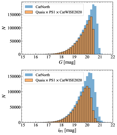
Figure 11: Upper panel: histograms of the apparent $G$ magnitudes of CatNorth (blue bars) and the Quaia subsample with PS1 and CatWISE2020 data (Quaia $\times$ PS1 $\times$ CatWISE2020; filled orange step plot). Lower panel: same as the upper panel, but for apparent $i_{\mathrm{P1}}$ magnitudes.

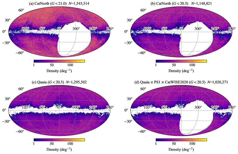
Figure 12: HEALPix (Górski et al., 2005) sky density maps of the CatNorth quasar candidate catalog (a), the CatNorth subsample with $G<20.5$ (b), the full Quaia catalog (c), and the Quaia subsample with PS1 and CatWISE2020 data (d). The maps are plotted in Galactic coordinates, with parameter $N_{\mathrm{side}}=64$ and an area of 0.839 $\mathrm{deg}^{2}$ per pixel.

7.2 Performance of the CatNorth catalog

To compare the intrinsic brightness of the CatNorth quasar candidates and the SDSS DR16Q sample, we calculate the SDSS $i$-band absolute magnitude $\mathrm{M}_{i}$ normalized at $z=2$ of the two samples. Because SDSS photometry is unavailable for most of the CatNorth sources, we first convert the $i_{\rm P1}$ magnitude to the $i_{\rm SDSS}$ magnitude with the transformations from Tonry et al. (2012). Then we correct for Galactic extinction for the converted $i_{\rm SDSS}$ with the two-dimensional dust map from Planck Collaboration et al. (2016) and the extinction law from Wang & Chen (2019). The absolute magnitudes $\mathrm{M}_{i}(z=2)$ are calculated with the $K$-correction (see e.g. Oke & Sandage, 1968; Hogg et al., 2002; Blanton & Roweis, 2007) values for the SDSS $i$ band from Richards et al. (2006).

The absolute magnitudes $\mathrm{M}_{i}(z=2)$ and redshift distributions of CatNorth and the DR16Q redshift subsample (421,959 sources, see Section 2.3.1) are shown in Figure 13, where photometric redshift values are used for CatNorth and spectroscopic redshifts from WS22 are used for DR16Q. In general, the CatNorth sources are brighter than the DR16Q sources, because the Gaia photometry is shallower than that of SDSS, and the target selections of SDSS quasars are biased towards fainter and higher-redshift ends than this work. Because we use the corrected flux excess factor $C^{*}$ to quantify the source extent in the classification model, instead of selecting only “point sources” using a single criterion (e.g. type=6 in the SDSS database; Richards et al., 2009), our quasar candidates are less biased in source extent than the SDSS quasars. Therefore we expect higher completeness in CatNorth than DR16Q in the bright end and low redshift (e.g. $z<0.5$).

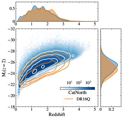
Figure 13: The absolute magnitudes $\mathrm{M}_{i}(z=2)$ and redshift distributions of the CatNorth catalog and the DR16Q subsample with good redshifts with 421,959 sources. In the main panel (lower left), the CatNorth sources are shown as the two-dimensional histogram (density plot), over which the white contour lines based on two-dimensional kernel density estimation (KDE) are plotted. The DR16Q sources are shown as orange KDE contours. In the top and right panels, the blue-shaded areas denote the KDE probability density functions of the CatNorth catalog, and the orange-shaded areas denote the probability densities of the DR16Q sample.

The color-magnitude or color-color properties of the CatNorth and DR16Q sources are shown in Figure 14. In general, CatNorth sources have color-color distributions that are well matched to those of DR16Q, except that CatNorth extends more into the red regimes than DR16Q. The consistency of the color distributions of the two samples implies a low level of contamination from stars and galaxies in CatNorth. The larger coverage of CatNorth in the red regimes compared to DR16Q may be due to the higher completeness of CatNorth, or a better sky coverage of Gaia in low Galactic latitude regions with large extinctions (see e.g. Fu et al., 2021).

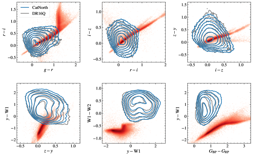
Figure 14: Color-color diagrams of sources from the CatNorth quasar candidate catalog (blue contours), 200,000 SDSS DR16Q quasars (gray contours), and 400,000 stars (red-shaded density plots) using photometric data from PS1, CatWISE2020 and Gaia DR3. The SDSS DR16Q subset and the star sample are the same as those in Figure 3. All magnitudes are in the AB system.

To further examine the reliability of the CatNorth quasar candidates, we used the 2-m HCT telescope of the Indian Astronomical Observatory to identify a random sample of CatNorth that is (i) not in the Quaia catalog, and (ii) not identified previously. The observation was made on Aug. 16, 2023. Ten candidates have been observed, which are randomly selected from a parent sample defined as:

    (ra>202.5 OR ra<60) AND log_fpm0<99 AND
    i_mean_psf_mag<17.5 AND dec>-10.

Out of the ten objects, eight are identified as quasars, one is identified as a star, and one is unknown (see Figure 15 for their spectra). The high success rate of 80% of the random observation proves the high purity of even the CatNorth sources that are missed by Quaia. We conclude that the CatNorth catalog has both high purity ($\sim 90\%$) and completeness, which is valuable for cosmological applications and follow-up identifications.

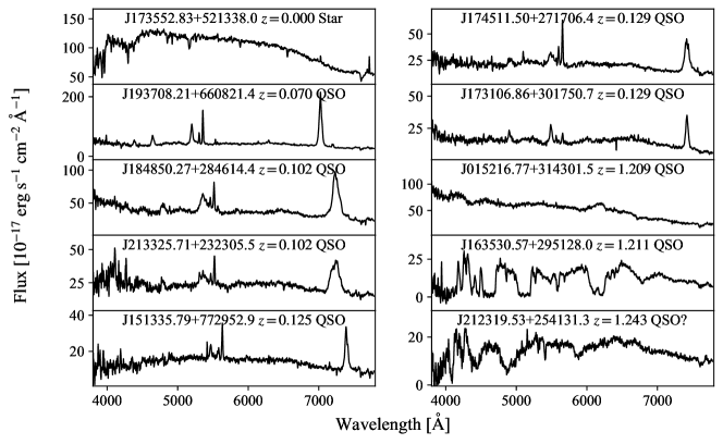
Figure 15: The HCT spectra of ten randomly selected CatNorth quasar candidates that are not in Quaia.

8 Summary and conclusions

In this paper, we present CatNorth, an improved Gaia DR3 quasar candidate catalog based on data from Gaia DR3, PS1, and CatWISE2020. We propose an ensemble machine learning classification approach to select quasar candidates, which are built on well-defined samples of quasars, galaxies, and two master stellar samples. The master stellar sample LVAC_PLUS is mainly based on the LAMOST value-added catalogs, while the other master stellar sample GDR3_PLUS is mainly based on the Gaia DR3 stellar samples. The two master stellar samples also include a mutual sample of very low-mass stars, white dwarfs, and carbon stars from the literature. By keeping the extragalactic samples fixed and alternating between two master samples of stars, we compose two sets of training/validation data using the 14 photometric features selected in Section 3. With the two training sets, two XGBoost classification models are trained using optimal hyperparameters given by the optuna software. An ensemble classification model is obtained by averaging the predicted probabilities of the two base classification models.

Using a probability threshold of $p_{\mathrm{QSO\_mean}}>0.95$ on our ensemble XGBoost classification model and an additional proper motion cut of $\log(f_{\mathrm{PM0}})\geq-4$, we retrieved 1,545,514 reliable quasar candidates (CatNorth catalog) from the parent sample of Gaia DR3 QSO candidates. We used XGBoost, TabNet and FT-Transformer to train an ensemble regression model to estimate photometric redshifts ($z_{\rm ph}$) from multi-band photometry and the lower and upper confidence intervals of Gaia redshifts. For candidates with Gaia BP/RP spectra, we also estimated their spectral redshifts ($z_{\rm xp\_nn}$) with the CNN-based RegNet model. As discussed in Section 6.3, $z_{\rm ph}$ and $z_{\rm xp\_nn}$ are highly consistent with each other, showing significant improvement over the original redshifts of Gaia.

The CatNorth catalog has limiting magnitudes of $G\lesssim 21$ and $i_{\mathrm{P1}}\lesssim 21.5$, and it shows color-color distributions that are well-matched to those of SDSS DR16Q. Nevertheless, the CatNorth sources are overall brighter than the DR16Q quasars because of the shallower depth of Gaia. The CatNorth catalog is also more complete in the low-redshift and red regimes in comparison to DR16Q. Compared to the Quaia catalog, the CatNorth catalog has similar purity ($\sim 90\%$) and higher completeness. This is proved by our latest spectroscopic identifications of eight new quasars from a random sample of ten candidates that are not in Quaia.

The CatNorth catalog is used as the main source of input catalog for the LAMOST phase III quasar survey, along with the candidate catalog of quasars behind the Galactic plane (Fu et al., 2021), the BASS DR3 quasar candidates (Li et al., 2021a), and the quasar candidates selected with PS1 variability (Hernitschek et al., 2016). By adding quasar candidates from different catalogs, LAMOST is expected to build a highly complete sample of bright quasars with $i<19.5$.

The next phase of this project involves the creation of an improved Gaia DR3 quasar candidate catalog covering the entire southern hemisphere. Accurate photometric and spectroscopic redshifts will also be provided for the southern quasar candidate sample. This project and surveys including LAMOST and the All-sky BRIght, Complete Quasar Survey (AllBRICQS; Onken et al., 2023) are of paramount importance in advancing cosmological studies, particularly concerning bright quasars.

9 ADQL queries for selecting Gaia DR3 stellar samples

9.1 The Gaia DR3 OBA sample

SELECT gs.source_id, gs.ra, gs.dec, l, b,
parallax, parallax_error, parallax_over_error,
pm, pmra, pmra_error, pmdec, pmdec_error,
pmra_pmdec_corr, phot_g_mean_mag,
phot_bp_mean_mag, phot_rp_mean_mag,
phot_bp_rp_excess_factor,
astrometric_excess_noise,
astrometric_excess_noise_sig,
astrometric_params_solved,
ruwe, ipd_gof_harmonic_amplitude,
s.vtan_flag, gs.distance_gspphot,
ap.teff_esphs, ap.teff_esphs_uncertainty,
ap.spectraltype_esphs, ap.flags_esphs,
ps.obj_id AS ps_id, ps.ra AS ra_ps,
ps.dec AS dec_ps, ps.epoch_mean AS ps_epoch_mean,
ps.g_mean_psf_mag, ps.g_mean_psf_mag_error,
ps.r_mean_psf_mag, ps.r_mean_psf_mag_error,
ps.i_mean_psf_mag, ps.i_mean_psf_mag_error,
ps.z_mean_psf_mag, ps.z_mean_psf_mag_error,
ps.y_mean_psf_mag, ps.y_mean_psf_mag_error,
ps.n_detections as ps_n_detections,
xmatch.number_of_mates, xmatch.angular_distance,
xmatch.clean_panstarrs1_oid,
xmatch.number_of_neighbours
FROM gaiadr3.gaia_source AS gs
INNER JOIN gaiadr3.gold_sample_oba_stars
  AS s USING (source_id)
INNER JOIN gaiadr3.astrophysical_parameters
  AS ap USING (source_id)
JOIN gaiadr3.panstarrs1_best_neighbour
  AS xmatch USING (source_id)
JOIN gaiadr2.panstarrs1_original_valid AS ps
  ON xmatch.original_ext_source_id = ps.obj_id
WHERE ruwe < 1.4
AND astrometric_params_solved = 31
AND parallax_over_error > 10
AND ipd_frac_multi_peak < 6
AND phot_bp_n_blended_transits < 10
AND ap.teff_esphs > 7000
AND gs.classprob_dsc_combmod_star > 0.9
AND ps.g_mean_psf_mag > 14
AND ps.r_mean_psf_mag > 14
AND ps.i_mean_psf_mag > 14
AND ps.z_mean_psf_mag > 14
AND ps.y_mean_psf_mag > 14
AND ps.i_mean_psf_mag_error < 0.2171
AND s.vtan_flag = 0

9.2 The Gaia DR3 FGKM sample

SELECT gs.source_id, gs.ra, gs.dec, l, b,
parallax, parallax_error, parallax_over_error,
pm, pmra, pmra_error, pmdec, pmdec_error,
pmra_pmdec_corr, phot_g_mean_mag,
phot_bp_mean_mag, phot_rp_mean_mag,
phot_bp_rp_excess_factor,
astrometric_excess_noise,
astrometric_excess_noise_sig,
astrometric_params_solved,
ruwe, ipd_gof_harmonic_amplitude,
gs.teff_gspphot, teff_gspphot_marcs,
teff_gspphot_phoenix,
ps.obj_id AS ps_id, ps.ra AS ra_ps,
ps.dec AS dec_ps, ps.epoch_mean AS ps_epoch_mean,
ps.g_mean_psf_mag, ps.g_mean_psf_mag_error,
ps.r_mean_psf_mag, ps.r_mean_psf_mag_error,
ps.i_mean_psf_mag, ps.i_mean_psf_mag_error,
ps.z_mean_psf_mag, ps.z_mean_psf_mag_error,
ps.y_mean_psf_mag, ps.y_mean_psf_mag_error,
ps.n_detections as ps_n_detections,
xmatch.number_of_mates, xmatch.angular_distance,
xmatch.clean_panstarrs1_oid,
xmatch.number_of_neighbours
FROM gaiadr3.gaia_source AS gs
INNER JOIN gaiadr3.astrophysical_parameters
  AS ap USING (source_id)
JOIN gaiadr3.panstarrs1_best_neighbour
  AS xmatch USING (source_id)
JOIN gaiadr2.panstarrs1_original_valid AS ps
  ON xmatch.original_ext_source_id = ps.obj_id
WHERE ruwe < 1.4
AND astrometric_params_solved = 31
AND parallax_over_error > 15
AND ipd_frac_multi_peak < 6
AND phot_bp_n_blended_transits < 10
AND gs.teff_gspphot > 2500
AND gs.teff_gspphot < 7500
AND gs.distance_gspphot <
  1000/(parallax-4*parallax_error)
AND gs.distance_gspphot >
  1000/(parallax+4*parallax_error)
AND (gs.libname_gspphot=’MARCS’
  OR gs.libname_gspphot=’PHOENIX’)
AND ap.logposterior_gspphot > -4000
AND gs.classprob_dsc_combmod_star > 0.9
AND gs.mh_gspphot > -0.8
AND ABS(teff_gspphot_marcs -
  teff_gspphot_phoenix + 65) < 150
AND radius_gspphot < 100
AND mg_gspphot < 12
AND phot_bp_n_obs > 19
AND phot_rp_n_obs > 19
AND phot_g_n_obs > 150
AND ps.i_mean_psf_mag > 14
AND ps.i_mean_psf_mag_error < 0.2171
AND random_index BETWEEN 0 AND 450000000

References

- Abdurro’uf et al. (2022) Abdurro’uf, Accetta, K., Aerts, C., et al. 2022, ApJS, 259, 35, doi: 10.3847/1538-4365/ac4414
- Ai et al. (2016) Ai, Y. L., Wu, X.-B., Yang, J., et al. 2016, AJ, 151, 24, doi: 10.3847/0004-6256/151/2/24
- Akiba et al. (2019) Akiba, T., Sano, S., Yanase, T., Ohta, T., & Koyama, M. 2019, in Proceedings of the 25th ACM SIGKDD International Conference on Knowledge Discovery & Data Mining, KDD ’19 (New York, NY, USA: Association for Computing Machinery), 2623–2631, doi: 10.1145/3292500.3330701
- Alksnis et al. (2001) Alksnis, A., Balklavs, A., Dzervitis, U., et al. 2001, Baltic Astronomy, 10, 1, doi: 10.1515/astro-2001-1-202
- Andrae et al. (2023) Andrae, R., Fouesneau, M., Sordo, R., et al. 2023, A&A, 674, A27, doi: 10.1051/0004-6361/202243462
- Arik & Pfister (2021) Arik, S. Ö., & Pfister, T. 2021, Proceedings of the AAAI Conference on Artificial Intelligence, 35, 6679, doi: 10.1609/aaai.v35i8.16826
- Astropy Collaboration et al. (2013) Astropy Collaboration, Robitaille, T. P., Tollerud, E. J., et al. 2013, A&A, 558, A33, doi: 10.1051/0004-6361/201322068
- Astropy Collaboration et al. (2018) Astropy Collaboration, Price-Whelan, A. M., Sipőcz, B. M., et al. 2018, AJ, 156, 123, doi: 10.3847/1538-3881/aabc4f
- Astropy Collaboration et al. (2022) Astropy Collaboration, Price-Whelan, A. M., Lim, P. L., et al. 2022, ApJ, 935, 167, doi: 10.3847/1538-4357/ac7c74
- Bañados et al. (2018) Bañados, E., Venemans, B. P., Mazzucchelli, C., et al. 2018, Nature, 553, 473, doi: 10.1038/nature25180
- Bachchan et al. (2016) Bachchan, R. K., Hobbs, D., & Lindegren, L. 2016, A&A, 589, A71, doi: 10.1051/0004-6361/201527935
- Bailer-Jones (2011) Bailer-Jones, C. A. L. 2011, MNRAS, 411, 435, doi: 10.1111/j.1365-2966.2010.17699.x
- Best et al. (2021) Best, W. M. J., Liu, M. C., Magnier, E. A., & Dupuy, T. J. 2021, AJ, 161, 42, doi: 10.3847/1538-3881/abc893
- Blanton & Roweis (2007) Blanton, M. R., & Roweis, S. 2007, AJ, 133, 734, doi: 10.1086/510127
- Blanton et al. (2017) Blanton, M. R., Bershady, M. A., Abolfathi, B., et al. 2017, AJ, 154, 28, doi: 10.3847/1538-3881/aa7567
- Brammer et al. (2008) Brammer, G. B., van Dokkum, P. G., & Coppi, P. 2008, ApJ, 686, 1503, doi: 10.1086/591786
- Chambers et al. (2016) Chambers, K. C., Magnier, E. A., Metcalfe, N., et al. 2016, arXiv e-prints, arXiv:1612.05560. https://arxiv.org/abs/1612.05560
- Chen & Guestrin (2016) Chen, T., & Guestrin, C. 2016, in Proceedings of the 22nd ACM SIGKDD International Conference on Knowledge Discovery and Data Mining, KDD ’16 (New York, NY, USA: Association for Computing Machinery), 785–794, doi: 10.1145/2939672.2939785
- Christlieb et al. (2001) Christlieb, N., Green, P. J., Wisotzki, L., & Reimers, D. 2001, A&A, 375, 366, doi: 10.1051/0004-6361:20010814
- Creevey et al. (2023) Creevey, O. L., Sordo, R., Pailler, F., et al. 2023, A&A, 674, A26, doi: 10.1051/0004-6361/202243688
- Cristiani et al. (2023) Cristiani, S., Porru, M., Guarneri, F., et al. 2023, MNRAS, 522, 2019, doi: 10.1093/mnras/stad1007
- Cruz et al. (2023) Cruz, P., Cortés-Contreras, M., Solano, E., et al. 2023, MNRAS, 520, 4730, doi: 10.1093/mnras/stad353
- Cui et al. (2012) Cui, X.-Q., Zhao, Y.-H., Chu, Y.-Q., et al. 2012, Research in Astronomy and Astrophysics, 12, 1197, doi: 10.1088/1674-4527/12/9/003
- Dawson et al. (2013) Dawson, K. S., Schlegel, D. J., Ahn, C. P., et al. 2013, AJ, 145, 10, doi: 10.1088/0004-6256/145/1/10
- De Angeli et al. (2023) De Angeli, F., Weiler, M., Montegriffo, P., et al. 2023, A&A, 674, A2, doi: 10.1051/0004-6361/202243680
- Delchambre et al. (2023) Delchambre, L., Bailer-Jones, C. A. L., Bellas-Velidis, I., et al. 2023, A&A, 674, A31, doi: 10.1051/0004-6361/202243423
- Deng et al. (2012) Deng, L.-C., Newberg, H. J., Liu, C., et al. 2012, Research in Astronomy and Astrophysics, 12, 735, doi: 10.1088/1674-4527/12/7/003
- Di Matteo et al. (2005) Di Matteo, T., Springel, V., & Hernquist, L. 2005, Nature, 433, 604, doi: 10.1038/nature03335
- Dong et al. (2018) Dong, X. Y., Wu, X.-B., Ai, Y. L., et al. 2018, AJ, 155, 189, doi: 10.3847/1538-3881/aab5ae
- Downes et al. (2004) Downes, R. A., Margon, B., Anderson, S. F., et al. 2004, AJ, 127, 2838, doi: 10.1086/383211
- Dufour et al. (2017) Dufour, P., Blouin, S., Coutu, S., et al. 2017, in Astronomical Society of the Pacific Conference Series, Vol. 509, 20th European White Dwarf Workshop, ed. P. E. Tremblay, B. Gaensicke, & T. Marsh, 3, doi: 10.48550/arXiv.1610.00986
- Eisenstein et al. (2011) Eisenstein, D. J., Weinberg, D. H., Agol, E., et al. 2011, AJ, 142, 72, doi: 10.1088/0004-6256/142/3/72
- Faherty et al. (2009) Faherty, J. K., Burgasser, A. J., Cruz, K. L., et al. 2009, AJ, 137, 1, doi: 10.1088/0004-6256/137/1/1
- Fan et al. (2023) Fan, X., Bañados, E., & Simcoe, R. A. 2023, ARA&A, 61, 373, doi: 10.1146/annurev-astro-052920-102455
- Flesch (2021) Flesch, E. W. 2021, MNRAS, 504, 621, doi: 10.1093/mnras/stab812
- Flesch (2023) —. 2023, The Open Journal of Astrophysics, 6, 49, doi: 10.21105/astro.2308.01505
- Foreman-Mackey (2016) Foreman-Mackey, D. 2016, The Journal of Open Source Software, 1, 24, doi: 10.21105/joss.00024
- Fu (2020) Fu, Y. 2020, PyFOSC: a pipeline toolbox for BFOSC/YFOSC long-slit spectroscopy data reduction, v1.0.1, Zenodo, doi: 10.5281/zenodo.3915021
- Fu et al. (2021) Fu, Y., Wu, X.-B., Yang, Q., et al. 2021, ApJS, 254, 6, doi: 10.3847/1538-4365/abe85e
- Fu et al. (2022) Fu, Y., Wu, X.-B., Jiang, L., et al. 2022, ApJS, 261, 32, doi: 10.3847/1538-4365/ac7f3e
- Gaia Collaboration et al. (2018) Gaia Collaboration, Mignard, F., Klioner, S. A., et al. 2018, A&A, 616, A14, doi: 10.1051/0004-6361/201832916
- Gaia Collaboration et al. (2021) Gaia Collaboration, Brown, A. G. A., Vallenari, A., et al. 2021, A&A, 649, A1, doi: 10.1051/0004-6361/202039657
- Gaia Collaboration et al. (2022) Gaia Collaboration, Klioner, S. A., Lindegren, L., et al. 2022, A&A, 667, A148, doi: 10.1051/0004-6361/202243483
- Gaia Collaboration et al. (2023a) Gaia Collaboration, Vallenari, A., Brown, A. G. A., et al. 2023a, A&A, 674, A1, doi: 10.1051/0004-6361/202243940
- Gaia Collaboration et al. (2023b) Gaia Collaboration, Bailer-Jones, C. A. L., Teyssier, D., et al. 2023b, A&A, 674, A41, doi: 10.1051/0004-6361/202243232
- Gaia Collaboration et al. (2023c) Gaia Collaboration, Creevey, O. L., Sarro, L. M., et al. 2023c, A&A, 674, A39, doi: 10.1051/0004-6361/202243800
- Genest-Beaulieu & Bergeron (2019) Genest-Beaulieu, C., & Bergeron, P. 2019, ApJ, 882, 106, doi: 10.3847/1538-4357/ab379e
- Ginsburg et al. (2019) Ginsburg, A., Sipőcz, B. M., Brasseur, C. E., et al. 2019, AJ, 157, 98, doi: 10.3847/1538-3881/aafc33
- Girshick (2015) Girshick, R. B. 2015, CoRR, abs/1504.08083
- Gorishniy et al. (2021) Gorishniy, Y., Rubachev, I., Khrulkov, V., & Babenko, A. 2021, Advances in Neural Information Processing Systems, 34, 18932
- Górski et al. (2005) Górski, K. M., Hivon, E., Banday, A. J., et al. 2005, ApJ, 622, 759, doi: 10.1086/427976
- Green (2018) Green, G. 2018, The Journal of Open Source Software, 3, 695, doi: 10.21105/joss.00695
- Green (2013) Green, P. 2013, ApJ, 765, 12, doi: 10.1088/0004-637X/765/1/12
- Hawley et al. (2002) Hawley, S. L., Covey, K. R., Knapp, G. R., et al. 2002, AJ, 123, 3409, doi: 10.1086/340697
- Hernitschek et al. (2016) Hernitschek, N., Schlafly, E. F., Sesar, B., et al. 2016, ApJ, 817, 73, doi: 10.3847/0004-637X/817/1/73
- Hogg et al. (2002) Hogg, D. W., Baldry, I. K., Blanton, M. R., & Eisenstein, D. J. 2002, arXiv e-prints, astro. https://arxiv.org/abs/astro-ph/0210394
- Ilbert et al. (2006) Ilbert, O., Arnouts, S., McCracken, H. J., et al. 2006, A&A, 457, 841, doi: 10.1051/0004-6361:20065138
- Ji et al. (2016) Ji, W., Cui, W., Liu, C., et al. 2016, ApJS, 226, 1, doi: 10.3847/0067-0049/226/1/1
- Jiménez-Esteban et al. (2023) Jiménez-Esteban, F. M., Torres, S., Rebassa-Mansergas, A., et al. 2023, MNRAS, 518, 5106, doi: 10.1093/mnras/stac3382
- Jin et al. (2023) Jin, J.-J., Wu, X.-B., Fu, Y., et al. 2023, ApJS, 265, 25, doi: 10.3847/1538-4365/acaf89
- Jin et al. (2019) Jin, X., Zhang, Y., Zhang, J., et al. 2019, MNRAS, 485, 4539, doi: 10.1093/mnras/stz680
- Khramtsov et al. (2019) Khramtsov, V., Sergeyev, A., Spiniello, C., et al. 2019, A&A, 632, A56, doi: 10.1051/0004-6361/201936006
- Kleinman et al. (2013) Kleinman, S. J., Kepler, S. O., Koester, D., et al. 2013, ApJS, 204, 5, doi: 10.1088/0067-0049/204/1/5
- Koester & Kepler (2015) Koester, D., & Kepler, S. O. 2015, A&A, 583, A86, doi: 10.1051/0004-6361/201527169
- Kong et al. (2018) Kong, X., Luo, A. L., Li, X.-R., et al. 2018, PASP, 130, 084203, doi: 10.1088/1538-3873/aac7a8
- Kormendy & Ho (2013) Kormendy, J., & Ho, L. C. 2013, ARA&A, 51, 511, doi: 10.1146/annurev-astro-082708-101811
- Li et al. (2021a) Li, C., Zhang, Y., Cui, C., et al. 2021a, MNRAS, 506, 1651, doi: 10.1093/mnras/stab1650
- Li et al. (2021b) Li, J., Liu, C., Zhang, B., et al. 2021b, ApJS, 253, 45, doi: 10.3847/1538-4365/abe1c1
- Li et al. (2018) Li, Y.-B., Luo, A. L., Du, C.-D., et al. 2018, ApJS, 234, 31, doi: 10.3847/1538-4365/aaa415
- Liske et al. (2008) Liske, J., Grazian, A., Vanzella, E., et al. 2008, MNRAS, 386, 1192, doi: 10.1111/j.1365-2966.2008.13090.x
- Liu et al. (2020) Liu, C., Côté, P., Peng, E. W., et al. 2020, ApJS, 250, 17, doi: 10.3847/1538-4365/abad91
- Lodieu et al. (2017) Lodieu, N., Espinoza Contreras, M., Zapatero Osorio, M. R., et al. 2017, A&A, 598, A92, doi: 10.1051/0004-6361/201629410
- Luo et al. (2012) Luo, A. L., Zhang, H.-T., Zhao, Y.-H., et al. 2012, Research in Astronomy and Astrophysics, 12, 1243, doi: 10.1088/1674-4527/12/9/004
- Luo et al. (2015) Luo, A. L., Zhao, Y.-H., Zhao, G., et al. 2015, Research in Astronomy and Astrophysics, 15, 1095, doi: 10.1088/1674-4527/15/8/002
- Lyke et al. (2020) Lyke, B. W., Higley, A. N., McLane, J. N., et al. 2020, ApJS, 250, 8, doi: 10.3847/1538-4365/aba623
- Ma et al. (2009) Ma, C., Arias, E. F., Bianco, G., et al. 2009, IERS Technical Note, 35, 1
- Mainzer et al. (2011) Mainzer, A., Bauer, J., Grav, T., et al. 2011, ApJ, 731, 53, doi: 10.1088/0004-637X/731/1/53
- Makarov & Secrest (2022) Makarov, V. V., & Secrest, N. J. 2022, ApJ, 933, 28, doi: 10.3847/1538-4357/ac7047
- Marocco et al. (2020) Marocco, F., Eisenhardt, P. R. M., Fowler, J. W., et al. 2020, CatWISE2020 Catalog, IPAC, doi: 10.26131/IRSA551
- Marocco et al. (2021) —. 2021, ApJS, 253, 8, doi: 10.3847/1538-4365/abd805
- Mas-Buitrago et al. (2022) Mas-Buitrago, P., Solano, E., González-Marcos, A., et al. 2022, A&A, 666, A147, doi: 10.1051/0004-6361/202243895
- Meusinger et al. (2016) Meusinger, H., Schalldach, P., Mirhosseini, A., & Pertermann, F. 2016, A&A, 587, A83, doi: 10.1051/0004-6361/201527277
- Mignard et al. (2016) Mignard, F., Klioner, S., Lindegren, L., et al. 2016, A&A, 595, A5, doi: 10.1051/0004-6361/201629534
- Nakoneczny et al. (2021) Nakoneczny, S. J., Bilicki, M., Pollo, A., et al. 2021, A&A, 649, A81, doi: 10.1051/0004-6361/202039684
- Odland (2018) Odland, T. 2018, tommyod/KDEpy: Kernel Density Estimation in Python, v0.9.10, Zenodo, doi: 10.5281/zenodo.2392268
- Oke & Sandage (1968) Oke, J. B., & Sandage, A. 1968, ApJ, 154, 21, doi: 10.1086/149737
- Onken et al. (2023) Onken, C. A., Wolf, C., Hon, W. J., et al. 2023, PASA, 40, e010, doi: 10.1017/pasa.2023.7
- Pâris et al. (2017) Pâris, I., Petitjean, P., Ross, N. P., et al. 2017, A&A, 597, A79, doi: 10.1051/0004-6361/201527999
- Pedregosa et al. (2011) Pedregosa, F., Varoquaux, G., Gramfort, A., et al. 2011, Journal of Machine Learning Research, 12, 2825. http://jmlr.org/papers/v12/pedregosa11a.html
- Pelletier et al. (1986) Pelletier, C., Fontaine, G., Wesemael, F., Michaud, G., & Wegner, G. 1986, ApJ, 307, 242, doi: 10.1086/164410
- Planck Collaboration et al. (2016) Planck Collaboration, Aghanim, N., Ashdown, M., et al. 2016, A&A, 596, A109, doi: 10.1051/0004-6361/201629022
- Rees (1986) Rees, M. J. 1986, MNRAS, 218, 25P, doi: 10.1093/mnras/218.1.25P
- Richards et al. (2002) Richards, G. T., Fan, X., Newberg, H. J., et al. 2002, AJ, 123, 2945, doi: 10.1086/340187
- Richards et al. (2006) Richards, G. T., Strauss, M. A., Fan, X., et al. 2006, AJ, 131, 2766, doi: 10.1086/503559
- Richards et al. (2009) Richards, G. T., Myers, A. D., Gray, A. G., et al. 2009, ApJS, 180, 67, doi: 10.1088/0067-0049/180/1/67
- Riello et al. (2021) Riello, M., De Angeli, F., Evans, D. W., et al. 2021, A&A, 649, A3, doi: 10.1051/0004-6361/202039587
- Risaliti & Lusso (2015) Risaliti, G., & Lusso, E. 2015, ApJ, 815, 33, doi: 10.1088/0004-637X/815/1/33
- Risaliti & Lusso (2019) —. 2019, Nature Astronomy, 3, 272, doi: 10.1038/s41550-018-0657-z
- Ruz-Mieres (2023) Ruz-Mieres, D. 2023, gaia-dpci/GaiaXPy: GaiaXPy 2.0.1, 2.0.1, Zenodo, doi: 10.5281/zenodo.7566303
- Sagi & Rokach (2018) Sagi, O., & Rokach, L. 2018, WIREs Data Mining and Knowledge Discovery, 8, e1249, doi: https://doi.org/10.1002/widm.1249
- Sandage (1962) Sandage, A. 1962, ApJ, 136, 319, doi: 10.1086/147385
- Sarro et al. (2023) Sarro, L. M., Berihuete, A., Smart, R. L., et al. 2023, A&A, 669, A139, doi: 10.1051/0004-6361/202244507
- Shen et al. (2016) Shen, S.-Y., Argudo-Fernández, M., Chen, L., et al. 2016, Research in Astronomy and Astrophysics, 16, 43, doi: 10.1088/1674-4527/16/3/043
- Si et al. (2015) Si, J.-M., Li, Y.-B., Luo, A. L., et al. 2015, Research in Astronomy and Astrophysics, 15, 1671, doi: 10.1088/1674-4527/15/10/005
- Skrzypek et al. (2016) Skrzypek, N., Warren, S. J., & Faherty, J. K. 2016, A&A, 589, A49, doi: 10.1051/0004-6361/201527359
- Storey-Fisher et al. (2023) Storey-Fisher, K., Hogg, D. W., Rix, H.-W., et al. 2023, arXiv e-prints, arXiv:2306.17749, doi: 10.48550/arXiv.2306.17749
- STScI (2022) STScI. 2022, Pan-STARRS1 DR1 Catalog, STScI/MAST, doi: 10.17909/55E7-5X63
- Su & Cui (2004) Su, D.-Q., & Cui, X.-Q. 2004, Chinese J. Astron. Astrophys., 4, 1, doi: 10.1088/1009-9271/4/1/1
- Tange (2018) Tange, O. 2018, GNU Parallel 2018 (Ole Tange), doi: 10.5281/zenodo.1146014
- Taylor (2005) Taylor, M. B. 2005, in Astronomical Society of the Pacific Conference Series, Vol. 347, Astronomical Data Analysis Software and Systems XIV, ed. P. Shopbell, M. Britton, & R. Ebert, 29
- The Pandas Development Team (2022) The Pandas Development Team. 2022, pandas-dev/pandas: Pandas, v1.5.0, Zenodo, Zenodo, doi: 10.5281/zenodo.7093122
- Tonry et al. (2012) Tonry, J. L., Stubbs, C. W., Lykke, K. R., et al. 2012, ApJ, 750, 99, doi: 10.1088/0004-637X/750/2/99
- Trump et al. (2006) Trump, J. R., Hall, P. B., Reichard, T. A., et al. 2006, ApJS, 165, 1, doi: 10.1086/503834
- Vanden Berk et al. (2001) Vanden Berk, D. E., Richards, G. T., Bauer, A., et al. 2001, AJ, 122, 549, doi: 10.1086/321167
- Wang & Chen (2019) Wang, S., & Chen, X. 2019, ApJ, 877, 116, doi: 10.3847/1538-4357/ab1c61
- Wang et al. (1996) Wang, S.-g., Su, D.-q., Chu, Y.-q., Cui, X., & Wang, Y.-n. 1996, Applied Optics, 35, 5155
- Wang et al. (2022) Wang, Y.-F., Luo, A. L., Chen, W.-P., et al. 2022, A&A, 660, A38, doi: 10.1051/0004-6361/202142009
- Wenzl et al. (2021) Wenzl, L., Schindler, J.-T., Fan, X., et al. 2021, AJ, 162, 72, doi: 10.3847/1538-3881/ac0254
- Wes McKinney (2010) Wes McKinney. 2010, in Proceedings of the 9th Python in Science Conference, ed. Stéfan van der Walt & Jarrod Millman, 56 – 61, doi: 10.25080/Majora-92bf1922-00a
- West et al. (2011) West, A. A., Morgan, D. P., Bochanski, J. J., et al. 2011, AJ, 141, 97, doi: 10.1088/0004-6256/141/3/97
- Weymann et al. (1981) Weymann, R. J., Carswell, R. F., & Smith, M. G. 1981, ARA&A, 19, 41, doi: 10.1146/annurev.aa.19.090181.000353
- Wright et al. (2010) Wright, E. L., Eisenhardt, P. R. M., Mainzer, A. K., et al. 2010, AJ, 140, 1868, doi: 10.1088/0004-6256/140/6/1868
- Wu & Shen (2022) Wu, Q., & Shen, Y. 2022, ApJS, 263, 42, doi: 10.3847/1538-4365/ac9ead
- Wu et al. (2015) Wu, X.-B., Wang, F., Fan, X., et al. 2015, Nature, 518, 512, doi: 10.1038/nature14241
- Xiang et al. (2019) Xiang, M., Ting, Y.-S., Rix, H.-W., et al. 2019, ApJS, 245, 34, doi: 10.3847/1538-4365/ab5364
- Xiang et al. (2022) Xiang, M., Rix, H.-W., Ting, Y.-S., et al. 2022, A&A, 662, A66, doi: 10.1051/0004-6361/202141570
- Yao et al. (2019) Yao, S., Wu, X.-B., Ai, Y. L., et al. 2019, ApJS, 240, 6, doi: 10.3847/1538-4365/aaef88
- York et al. (2000) York, D. G., Adelman, J., Anderson, John E., J., et al. 2000, AJ, 120, 1579, doi: 10.1086/301513
- Yuan et al. (2015) Yuan, H. B., Liu, X. W., Huo, Z. Y., et al. 2015, MNRAS, 448, 855, doi: 10.1093/mnras/stu2723
- Zhang et al. (2019) Zhang, S., Luo, A. L., Comte, G., et al. 2019, ApJS, 240, 31, doi: 10.3847/1538-4365/aafb32
- Zhang et al. (2021) —. 2021, ApJ, 908, 131, doi: 10.3847/1538-4357/abcfc5
- Zhang et al. (2018) Zhang, Z. H., Galvez-Ortiz, M. C., Pinfield, D. J., et al. 2018, MNRAS, 480, 5447, doi: 10.1093/mnras/sty2054
- Zhao et al. (2012) Zhao, G., Zhao, Y.-H., Chu, Y.-Q., Jing, Y.-P., & Deng, L.-C. 2012, Research in Astronomy and Astrophysics, 12, 723, doi: 10.1088/1674-4527/12/7/002
- Zonca et al. (2019) Zonca, A., Singer, L., Lenz, D., et al. 2019, The Journal of Open Source Software, 4, 1298, doi: 10.21105/joss.01298