Stable Recovery of Coefficients in an Inverse Fault Friction Problem

Abstract.

We consider the inverse fault friction problem of determining the friction coefficient in the Tresca friction model, which can be formulated as an inverse problem for differential inequalities. We show that the measurements of elastic waves during a rupture uniquely determine the friction coefficient at the rupture surface with explicit stability estimates.

1. Introduction

The study of earthquake physics remains highly challenging through its complex dynamics and multifaceted nature. Nearly all aspects of earthquake ruptures are controlled by the friction along a fault, where these commonly occur, that progressively increases with tectonic forcing. Indeed, in a recent Annual Review of Earth and Planetary Sciences, it was stated that “determining the friction during an earthquake is required to understand when and where earthquakes occur” (Brodsky et al. [1]). Some common approach has been developed retrieving the stress evolution at each point of the fault as dictated by the slip history obtained from the kinematic inverse rupture problem; we mention work by Ide and Takeo [12], who determined the spatiotemporal slip distribution on an assumed fault plane of the 1995 Kobe earthquake by “waveform inversion” and then numerically solved the elastodynamic equations to determine the stress distribution and constitutive relations on the fault plane. However, seismologists studying earthquake dynamics have reported that both stress and friction on a fault are still poorly known and difficult to constrain with observations (Causse, Dalguer and Mai [2]). Here, we address the question whether this is possible, in principle.

We study the recovery of a time- and space-dependent friction coefficient via the slip rate and normal and tangential stresses, using the Tresca model (see e.g. the book of Sofonea and Matei [17]), at a pre-existing fault from “near-surface” elastic-wave, that is, seismic displacement data. This dynamic inverse friction problem can be regarded as an inverse problem for differential inequalities, as the Tresca friction model can be formulated through variational inequalities as seen in many contact mechanics problems (e.g. [4, 17]). While inverse problems for differential equations have been widely studied, inverse problems for differential inequalities have not yet received much attention. Our approach is based on the quantitative unique continuation for the elastic wave equation established in our recent work [3], where we studied the kinematic inverse rupture problem of determining the friction force at the rupture surface from seismic displacement data. Itou and Kashiwabara [13] recently analyzed the Tresca model on a fault coupled to the elastic wave equation; we exploit their results in our study of the inverse problem. As a disclaimer, while we address the most fundamental question, we do ignore more complex physics such as thermo-mechanical effects.

We remark that in the past two decades, quite many studies have been devoted to the practical determination of fault frictional properties by analyzing slowly-evolving afterslip following large earthquakes. For very recent results, see Zhao and Yue [20]. Afterslip is the fault slip process in response to an instantaneous coseismic stress change, in which the slip velocity decrease corresponds to the stress releasing by itself. Its “self-driven” nature provides a framework to model the slip process with the fault frictional properties alone. For a review, see Yue et al. [19]. Afterslip is analyzed with quasi-static deformation, that is, with the elastostatic system of equations, typically using geodetic data.

Let $M$ be the solid Earth and $\Sigma_{{\rm f}}$ be a rupture surface. Consider the elastic wave equation

(1) $$\rho\partial_{t}^{2}\boldsymbol{u}-\mu\Delta\boldsymbol{u}-(\lambda+\mu)\nabla(\nabla\cdot\boldsymbol{u})=0\quad\textrm{in }\big{(}M\setminus\overline{{\Sigma}_{\mathrm{f}}}\big{)}\times(-T,T)\,,$$

with the Tresca friction condition (e.g. [4, 13, 14]) on the rupture surface $\Sigma_{{\rm f}}$:

(2) $$\left\{\begin{aligned} &\sigma_{n}=F_{n}\,\textrm{ is given},\\ &|\boldsymbol{\sigma}_{\tau}|<g\Longrightarrow{\,[\,\partial_{t}\boldsymbol{u}_{\tau}\,]_{-}^{+}}=0,\\ &|\boldsymbol{\sigma}_{\tau}|=g\Longrightarrow{\,[\,\partial_{t}\boldsymbol{u}_{\tau}\,]_{-}^{+}}\cdot\boldsymbol{\sigma}_{\tau}=g\,\big{|}{\,[\,\partial_{t}\boldsymbol{u}_{\tau}\,]_{-}^{+}}\big{|}\,.\end{aligned}\right.$$

Here $\sigma_{n}=(\boldsymbol{\sigma}(\boldsymbol{u}){\boldsymbol{n}})\cdot{\boldsymbol{n}}$ and $\boldsymbol{\sigma}_{\tau}=\boldsymbol{\sigma}(\boldsymbol{u}){\boldsymbol{n}}-\sigma_{n}{\boldsymbol{n}}$ are the normal and tangential components of the stress tensor $\boldsymbol{\sigma}(\boldsymbol{u})$, where ${\boldsymbol{n}}$ is the unit normal vector of the rupture surface $\Sigma_{{\rm f}}$. The stress tensor $\boldsymbol{\sigma}(\boldsymbol{u})$ is defined as

(3) $$\boldsymbol{\sigma}(\boldsymbol{u})=2\mu\boldsymbol{\varepsilon}(\boldsymbol{u})+\lambda\big{(}{\rm tr}\,\boldsymbol{\varepsilon}(\boldsymbol{u})\big{)}\boldsymbol{I},\quad\;\boldsymbol{\varepsilon}(\boldsymbol{u})=\frac{1}{2}\Big{(}\nabla\boldsymbol{u}+(\nabla\boldsymbol{u})^{T}\Big{)}.$$

The notation ${\,[\,\cdot\,]_{-}^{+}}$ stands for the jump across the rupture surface, more precisely,

(4) $${\,[\,\partial_{t}\boldsymbol{u}_{\tau}\,]_{-}^{+}}:=\partial_{t}(\boldsymbol{u}_{\tau}^{+}-\boldsymbol{u}_{\tau}^{-}),\quad\boldsymbol{u}_{\tau}^{\pm}:=\lim_{h\to 0^{\pm}}\boldsymbol{u}_{\tau}(z+h{\boldsymbol{n}},t),\quad z\in\Sigma_{{\rm f}},$$

where $\boldsymbol{u}_{\tau}$ is the tangential component of $\boldsymbol{u}$. The friction force $g$ at $\Sigma_{{\rm f}}$ is of the form

(5) $$g=\mathscr{F}|F_{n}|,$$

where $\mathscr{F}$ is the friction coefficient. Note that the friction force $g$ and the friction coefficient $\mathscr{F}$ may depend on time.

Regarding the direct problem for the Tresca friction model above, the weak formulation is understood in the variational sense (see e.g. [13, 4, 17]). Recall that with the Dirichlet condition on the boundary $\partial M$, the problem of finding $\boldsymbol{u}$ satisfying the Tresca friction model (1-2) is formulated as finding $\boldsymbol{u}$ such that for all $\boldsymbol{v}\in H^{1}(M\setminus\overline{{\Sigma}_{\mathrm{f}}})$ and all $t\in(0,T)$, the following variational inequality holds:

(6) $$\rho\int_{M\setminus\overline{{\Sigma}_{\mathrm{f}}}}(\boldsymbol{v}-\partial_{t}\boldsymbol{u})\partial_{t}^{2}\boldsymbol{u}\,dV+a\big{(}\boldsymbol{u},\boldsymbol{v}-\partial_{t}\boldsymbol{u}\big{)}$$

$$+\int_{{\Sigma}_{\mathrm{f}}}g\cdot\big{|}{\,[\,\boldsymbol{v}_{\tau}\,]_{-}^{+}}\big{|}\,dA-\int_{{\Sigma}_{\mathrm{f}}}g\cdot\big{|}{\,[\,\partial_{t}\boldsymbol{u}_{\tau}\,]_{-}^{+}}\big{|}\,dA+\int_{{\Sigma}_{\mathrm{f}}}F_{n}\cdot{\,[\,v_{n}\,]_{-}^{+}}\,dA\geq 0,$$

where $dV,\,dA$ stand for the volume and area element of $M$ and ${\Sigma}_{\mathrm{f}}$, respectively, and $a$ is a bilinear symmetric form defined by $a(\boldsymbol{v},\boldsymbol{w}):=\int_{M\setminus\overline{{\Sigma}_{\mathrm{f}}}}\textrm{tr}\big{(}\boldsymbol{\sigma}(\boldsymbol{v})^{T}\boldsymbol{\varepsilon}(\boldsymbol{w})\big{)}\,dV$. If one assumes

$$\boldsymbol{u}_{0}:=\boldsymbol{u}(\cdot,0)\in H^{1}(M\setminus\overline{{\Sigma}_{\mathrm{f}}}),\quad\partial_{t}\boldsymbol{u}(\cdot,0)\in H^{1}(M\setminus\overline{{\Sigma}_{\mathrm{f}}}),$$

$$F_{n}\in H^{2}(0,T;L^{2}({\Sigma}_{\mathrm{f}})),\quad g\in H^{2}(0,T;L^{2}({\Sigma}_{\mathrm{f}})),$$

and the compatibility conditions at $t=0$:

$$\left\{\begin{aligned} &\textrm{div}\,\boldsymbol{\sigma}(\boldsymbol{u}_{0})\in L^{2}(M\setminus\overline{{\Sigma}_{\mathrm{f}}}),\\ &\sigma_{n}(\boldsymbol{u}_{0}^{+})=\sigma_{n}(\boldsymbol{u}_{0}^{-})=F_{n}(\cdot,0)\quad&\textrm{ on }{\Sigma}_{\mathrm{f}},\\ &\boldsymbol{\sigma}_{\tau}(\boldsymbol{u}_{0}^{+})=\boldsymbol{\sigma}_{\tau}(\boldsymbol{u}_{0}^{-})=0,\;\;\partial_{t}\boldsymbol{u}_{\tau}(\cdot,0)=0\quad&\textrm{ on }{\Sigma}_{\mathrm{f}},\end{aligned}\right.$$

then the friction problem above has a unique solution [13],

(7) $$\boldsymbol{u}\in W^{1,\infty}\big{(}0,T;H^{1}(M\setminus\overline{{\Sigma}_{\mathrm{f}}})\big{)}\cap W^{2,\infty}\big{(}0,T;L^{2}(M\setminus\overline{{\Sigma}_{\mathrm{f}}})\big{)}.$$

In this paper, we consider the inverse problem of determining the friction coefficient $\mathscr{F}$ in the Tresca friction model above. For the sake of presentation, we consider the elastic wave equation (1) on the time interval $(-T,T)$. Denote the a priori bound for the norm of $\boldsymbol{u}$ in the space (7) by

(8) $$\|\boldsymbol{u}\|_{W^{1,\infty}(-T,T;H^{1})}+\|\boldsymbol{u}\|_{W^{2,\infty}(-T,T;L^{2})}\leq\Lambda_{0}.$$

We impose the following assumption on the regularity of the normal stress $F_{n}$ and the friction coefficient $\mathscr{F}$. Assume that $F_{n}\in H^{s}(\Sigma_{{\rm f}}\times[-T,T])$ for some $s\in(0,1]$ and $\mathscr{F}\in C^{0,1}(\Sigma_{{\rm f}}\times[-T,T])$, and

(9) $$0<c_{0}\leq F_{n}\leq C_{0},\quad\|F_{n}\|_{H^{s}(\Sigma_{{\rm f}}\times[-T,T])}\leq C_{0},\quad\|\mathscr{F}\|_{C^{0,1}(\Sigma_{{\rm f}}\times[-T,T])}\leq C_{0}.$$

In addition, assume that the parameters $\rho,\lambda,\mu$ in the elastic wave equation (1) to be smooth and time-independent on $M\setminus\overline{{\Sigma}_{\mathrm{f}}}$.

We prove the following result on the inverse fault friction problem during a rupture.

Theorem 1.

Let $M$ be the solid Earth with smooth boundary and $\Sigma_{{\rm f}}$ be a smooth rupture surface. Consider the elastic wave equation (1) with time-independent parameters and the Tresca friction condition (2). Assume the normal stress $F_{n}$ and the friction coefficient $\mathscr{F}$ satisfy (9) on $\Sigma_{{\rm f}}$. Assume ${\,[\,\partial_{t}\boldsymbol{u}_{\tau}\,]_{-}^{+}}\neq 0$ on $\Sigma_{{\rm f}}$ and a priori norm (8) for the elastic wave $\boldsymbol{u}$. Suppose we can measure the elastic wave $\boldsymbol{u}$ on an interior open set $U\subset M$ up to sufficiently large time $T$. Then we have the following conclusions.

1. The measurement of $\boldsymbol{u}$ on $U\times[-T,T]$ uniquely determines the friction coefficient $\mathscr{F}$ on $\Sigma_{{\rm f}}\times[-\frac{T}{2},\frac{T}{2}]$.

2. Suppose we have two systems with friction coefficients $\mathscr{F}_{1},\mathscr{F}_{2}$, and we can measure the corresponding elastic waves $\boldsymbol{u}_{1},\boldsymbol{u}_{2}$ on $U\times[-T,T]$. Then there exist constants $\widehat{\varepsilon_{0}},C,c$ such that for any $0<\varepsilon_{0}<\widehat{\varepsilon_{0}}$, if

   $$\|\boldsymbol{u}_{1}-\boldsymbol{u}_{2}\|_{H^{2}(U\times[-T,T])}\leq\varepsilon_{0},$$

   then the friction coefficients satisfy

   $$\|\mathscr{F}_{1}-\mathscr{F}_{2}\|_{L^{2}(\Sigma_{{\rm f}}\times[-\frac{T}{2},\frac{T}{2}])}\leq C(\log|\log\varepsilon_{0}|)^{-c},$$

   where the constants $\widehat{\varepsilon_{0}},C$ depend on $c_{0},C_{0},\Lambda_{0}$, parameters of the equation and geometric parameters of $M$, and $c$ depends only on $s$.

The proof of Theorem 1 is divided into two parts: the measurements of $\boldsymbol{u}$ on $U$ determine $\boldsymbol{u}$ near $\Sigma_{{\rm f}}$, and the latter determines $\mathscr{F}$ under the Tresca friction condition. The first part, also known as the kinematic inverse rupture problem [9], has mostly been done in our recent work [3]. Our method was based on the quantitative unique continuation for the elasticity system, motivated by [18, 6]. However, regularity issues remain: the actual regularity of waves is not enough for the quantitative unique continuation arguments to work on the whole domain, which is addressed in Section 2. The second part is discussed in Section 3.

2. Interior regularity

Let $M^{n}$ be a Riemannian manifold with boundary of dimension $n$. Let $\delta>0$ be small, and denote the interior by

(10) $$M_{\delta}:=\{x\in M:d(x,\partial M)\geq\delta\}.$$

Let $\boldsymbol{u}$ be an elastic wave satisfying the elastic wave equation (1). Recall [6, Lemma 5.1] that the elastic wave equation can be decomposed into a system of hyperbolic equations for $(\boldsymbol{u},\textrm{div}\,\boldsymbol{u},\textrm{curl}\,\boldsymbol{u})$. Let $U\subset M$ be a connected open subset. We choose $\delta$ sufficiently small such that $\overline{U}\subset M_{\delta}$.

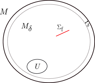
Figure 1. Setting of Lemma 2.1 and Proposition 2.2.

We apply Proposition 3.2 in [3] to $(\boldsymbol{u},\textrm{div}\,\boldsymbol{u},\textrm{curl}\,\boldsymbol{u})$ in $M_{\delta}$: for sufficiently small $h$ and sufficiently large $T$ (specified in [3, Proposition 3.2]), if

$$\|\boldsymbol{u}\|_{H^{2}(U\times[-T,T])}\leq\varepsilon_{0},$$

then

(11) $$\|\boldsymbol{u}\|_{L^{2}(M_{\delta}\times[-\frac{T}{2},\frac{T}{2}])}\leq C\exp(h^{-cn})\frac{\Lambda_{\delta}}{\Big{(}\log\big{(}1+h\frac{\Lambda_{\delta}}{\varepsilon_{0}}\big{)}\Big{)}^{\frac{1}{2}}}+C\Lambda_{0}h^{\frac{1}{n+1}},$$

where

(12) $$\Lambda_{\delta}:=\big{\|}(\boldsymbol{u},\textrm{div}\,\boldsymbol{u},\textrm{curl}\,\boldsymbol{u})\big{\|}_{H^{1}(M_{\delta}\times[-T,T])}.$$

Observe that $\Lambda_{\delta}$ essentially asks for $H^{2}$ regularity, while the solution of the direct problem (7) is only in $H^{1}$ in space. One way to resolve the issue is to use interior regularity estimate, and then use Sobolev embedding to get an immediate estimate for the boundary layer.

Lemma 2.1.

The following $H^{2}$ interior regularity estimate holds for the elastic wave equation (1):

$$\|\boldsymbol{u}\|_{H^{2}(M_{2\delta}\times[-T,T])}\leq C_{T}C_{M}\delta^{-4}\Big{(}\|\boldsymbol{u}\|_{W^{1,\infty}(-T,T;H^{1}(M))}+\|\boldsymbol{u}\|_{W^{2,\infty}(-T,T;L^{2}(M))}\Big{)},$$

which gives a bound

(13) $$\Lambda_{\delta}\leq C_{T}C_{M}\delta^{-4}\Lambda_{0},$$

where $C_{T}$ depends only on $T$, and $C_{M}$ depends only on geometric parameters of $M$.

Proof.

Suppose that $\varphi$ is a weak solution of the elliptic equation

$$\Delta\varphi=f,\quad\varphi\in H^{1}(M),\;f\in L^{2}(M).$$

Let $\chi$ be a cut-off function satisfying $\chi|_{M_{\delta}}=1$ and $\chi|_{\partial M}=0$. Then

$$\varphi_{0}:=\chi\varphi$$

satisfies

$$\left\{\begin{aligned} &\Delta\varphi_{0}=\chi\Delta\varphi+[\Delta,\chi]\varphi=:\widetilde{f},\\ &\varphi_{0}|_{\partial M}=0,\end{aligned}\right.$$

where

$$\|\widetilde{f}\|_{L^{2}(M)}\leq\delta^{-2}\Big{(}\|\varphi\|_{H^{1}(M)}+\|f\|_{L^{2}(M)}\Big{)}.$$

Hence $\varphi_{0}\in H^{2}(M)$ by boundary regularity for elliptic equations (e.g. [8, Theorem 4 in Chapter 6.3]). Then it follows that $\varphi|_{M_{\delta}}\in H^{2}(M_{\delta})$, and

(14) $$\|\varphi\|_{H^{2}(M_{\delta})}\leq\|\varphi_{0}\|_{H^{2}(M)}\leq C_{M}\delta^{-2}\Big{(}\|\varphi\|_{H^{1}(M)}+\|f\|_{L^{2}(M)}\Big{)}.$$

The constant $C_{M}$ depends on the first Dirichlet eigenvalue on $M$ which is uniformly bounded below by diameter and curvature bounds (e.g. [15, Theorem 8]). The same argument is valid for $\varphi\in L^{2}$ and $f\in H^{-1}$ with constant $C_{M}\delta^{-2}$.

Now we switch to the notations in our first paper

(15) $$(\boldsymbol{u},v,\boldsymbol{w}):=(\boldsymbol{u},\textrm{div}\,\boldsymbol{u},\textrm{curl}\,\boldsymbol{u}).$$

Recall that the elastic wave equation (1) can be decomposed into the following system ([6, Lemma 5.1] or [3, Lemma A.1]):

(16) $$\left\{\begin{aligned} &\frac{\rho}{\mu}\partial_{t}^{2}\boldsymbol{u}-\Delta\boldsymbol{u}+A_{1}(\boldsymbol{u},v)=0,\\ &\frac{\rho}{2\mu+\lambda}\partial_{t}^{2}v-\Delta v+A_{2}(\boldsymbol{u},v,\boldsymbol{w})=0,\\ &\frac{\rho}{\mu}\partial_{t}^{2}\boldsymbol{w}-\Delta\boldsymbol{w}+A_{3}(\boldsymbol{u},v,\boldsymbol{w})=0,\end{aligned}\right.$$

where $A_{i}$ are first order and has no time derivative.

Then consider the second equation. Since $\boldsymbol{u}\in W^{1,\infty}(-T,T;H^{1})$ from (7), then

$$v,\boldsymbol{w}\in W^{1,\infty}(-T,T;L^{2}),\quad A_{2}(\boldsymbol{u},v,\boldsymbol{w})\in W^{1,\infty}(-T,T;H^{-1}).$$

On the other hand, since $\boldsymbol{u}\in W^{2,\infty}(-T,T;L^{2})$ from (7), then

$$v\in W^{2,\infty}(-T,T;H^{-1}),\quad\partial_{t}^{2}v\in L^{\infty}(-T,T;H^{-1}).$$

Then using the second equation gives

$$\Delta v\in L^{\infty}(-T,T;H^{-1}).$$

Thus from the interior regularity argument (14) (for $L^{2}$-$H^{-1}$), we have

$$v|_{M_{\delta}}\in L^{\infty}(-T,T;H^{1})$$

with constant $C_{M}\delta^{-2}$ in the regularity estimate.

Next consider the first equation on $M_{\delta}$. Using the improved interior regularity for $v|_{M_{\delta}}$, we see that $A_{1}(\boldsymbol{u},v)|_{M_{\delta}}\in L^{\infty}(-T,T;L^{2})$. This gives

$$\Delta\boldsymbol{u}|_{M_{\delta}}\in L^{\infty}(-T,T;L^{2}),$$

considering that $\partial_{t}^{2}\boldsymbol{u}\in L^{\infty}(-T,T;L^{2})$. Thus by shrinking the domain by another $\delta$ and using (14), we obtain

$$\boldsymbol{u}|_{M_{2\delta}}\in L^{\infty}(-T,T;H^{2})$$

with constant $C_{M}\delta^{-4}$ in the regularity estimate, i.e.,

(17) $$\|\boldsymbol{u}\|_{L^{\infty}(-T,T;H^{2}(M_{2\delta}))}\leq C_{M}\delta^{-4}\Big{(}\|\boldsymbol{u}\|_{W^{1,\infty}(-T,T;H^{1}(M))}+\|\boldsymbol{u}\|_{W^{2,\infty}(-T,T;L^{2}(M))}\Big{)}.$$

Thus from (17) and (7), we obtain the estimate

$$\|\boldsymbol{u}\|_{H^{2}(M_{2\delta}\times[-T,T])} \leq C_{T}\Big{(}\|\boldsymbol{u}\|_{L^{\infty}(-T,T;H^{2}(M_{2\delta}))}+\|\boldsymbol{u}\|_{W^{1,\infty}(-T,T;H^{1}(M))}+\|\boldsymbol{u}\|_{W^{2,\infty}(-T,T;L^{2}(M))}\Big{)}$$

$$\leq C_{T}C_{M}\delta^{-4}\Big{(}\|\boldsymbol{u}\|_{W^{1,\infty}(-T,T;H^{1}(M))}+\|\boldsymbol{u}\|_{W^{2,\infty}(-T,T;L^{2}(M))}\Big{)}.$$

∎

Proposition 2.2.

Let $M$ be the solid Earth with smooth boundary and $U\subset M$ be a connected open set. Let $\boldsymbol{u}$ be an elastic wave with a priori norm (8). Then there exist constants $\widehat{\varepsilon_{0}},C,c$ such that for any $0<\varepsilon_{0}<\widehat{\varepsilon_{0}}$, if

$$\|\boldsymbol{u}\|_{H^{2}(U\times[-T,T])}\leq\varepsilon_{0},$$

then

$$\|\boldsymbol{u}\|_{L^{2}(M\times[-\frac{T}{2},\frac{T}{2}])}\leq C(\log|\log\varepsilon_{0}|)^{-c},$$

where the constants $\widehat{\varepsilon_{0}},C$ depend on $\Lambda_{0}$, parameters of the equation and geometric parameters of $M$, and $c$ is an absolute constant.

Proof.

From (11) and Lemma 2.1, using Sobolev embedding again to $M\setminus M_{\delta}$ gives

$$\|\boldsymbol{u}\|_{L^{2}(M\times[-\frac{T}{2},\frac{T}{2}])} \leq \|\boldsymbol{u}\|_{L^{2}(M_{\delta}\times[-\frac{T}{2},\frac{T}{2}])}+\|\boldsymbol{u}\|_{L^{2}((M\setminus M_{\delta})\times[-\frac{T}{2},\frac{T}{2}])}$$

$$\leq C\exp(h^{-cn})\frac{\delta^{-4}\Lambda_{0}}{\Big{(}\log\big{(}1+h\frac{\delta^{-4}\Lambda_{0}}{\varepsilon_{0}}\big{)}\Big{)}^{\frac{1}{2}}}+C\Lambda_{0}h^{\frac{1}{n+1}}+C\Lambda_{0}\delta^{\frac{1}{n+1}}.$$

From here, we need to balance the parameters $\delta,h,\varepsilon_{0}$. One can choose $\delta=h$ and $h=C(\log|\log\varepsilon_{0}|)^{-c}$, and then arrive at the desired formulation (see similar proof for [3, Corollary 1.2]). ∎

3. Inverse friction problem

Using Proposition 2.2, we consider the inverse problem of determining the friction coefficient $\mathscr{F}$ in the Tresca friction model.

Lemma 3.1.

Let $M$ be the solid Earth with smooth boundary, $\Sigma_{{\rm f}}$ be a smooth rupture surface, and $U\subset M$ be a connected open set. Let $\boldsymbol{u}$ be an elastic wave with a priori norm (8). If for sufficiently small $\varepsilon_{0}$,

$$\|\boldsymbol{u}\|_{H^{2}(U\times[-T,T])}\leq\varepsilon_{0},$$

then for any $\alpha\in(0,\frac{1}{2})$, we have

$$\big{\|}\boldsymbol{\sigma}(\boldsymbol{u})|_{\Sigma_{{\rm f}}}\big{\|}_{H^{-\frac{1}{2}-\alpha}(\Sigma_{{\rm f}}\times[-\frac{T}{2},\frac{T}{2}])}\leq C\Lambda_{0}^{1-\alpha}\varepsilon_{1}^{\alpha},$$

where $\varepsilon_{1}:=C(\log|\log\varepsilon_{0}|)^{-c}$. The same estimate also holds for the components $\sigma_{n},\boldsymbol{\sigma}_{\tau}$.

Proof.

Proposition 2.2 gives $\|\boldsymbol{u}\|_{L^{2}(M\times[-\frac{T}{2},\frac{T}{2}])}\leq\varepsilon_{1}$. We have a priori norm $\|\boldsymbol{u}\|_{H^{1}(M\times[-T,T])}\leq\Lambda_{0}$ by (8). By interpolation, we have

$$\|\boldsymbol{u}\|_{H^{1-\alpha}(M\times[-\frac{T}{2},\frac{T}{2}])}\leq\Lambda_{0}^{1-\alpha}\varepsilon_{1}^{\alpha}.$$

Recall the system (16) for $(\boldsymbol{u},v,\boldsymbol{w}):=(\boldsymbol{u},\textrm{div}\,\boldsymbol{u},\textrm{curl}\,\boldsymbol{u})$. Then

(18) $$\|v\|_{H^{-\alpha}(M\times[-\frac{T}{2},\frac{T}{2}])}+\|\boldsymbol{w}\|_{H^{-\alpha}(M\times[-\frac{T}{2},\frac{T}{2}])}\leq 2\Lambda_{0}^{1-\alpha}\varepsilon_{1}^{\alpha}.$$

To proceed further, we recall the $H_{(k,s)}$-norm in ${\mathbb{R}}^{n+1}$ (see [11, Definition B.1.10]) defined as

(19) $$\|u\|^{2}_{(k,s)}=\int_{{\mathbb{R}}^{n+1}}|\widehat{u}(\xi)|^{2}(1+|\xi|^{2})^{k}(1+|\xi^{\prime}|^{2})^{s}d\xi\,,$$

with respect to the coordinates $y=(x^{\prime},x^{n})\in{\mathbb{R}}^{n}\times{\mathbb{R}}$. Note that when $s=0$, the $H_{(k,0)}$-norm above is equivalent to the usual $H^{k}$-norm. The idea is using partial hypoellipticity (e.g. [11, Appendix B] or [7, Chapter 26.1]) to trade regularity between normal and tangential components.

Using the notation (19), since $v,\boldsymbol{w}\in H_{(-\alpha,0)}$ from (18) and thus $P_{2}v=-A_{2}(\boldsymbol{u},v,\boldsymbol{w})\in H_{(-1-\alpha,0)}$ where $P_{2}=\frac{\rho}{2\mu+\lambda}\partial_{t}^{2}-\Delta$ by the second equation in (16), then [11, Theorem B.2.9] gives $v\in H_{(1-\alpha,-1)}$ with norm estimate:

$$\|v\|_{(1-\alpha,-1)} \leq C\Big{(}\|v\|_{(-\alpha,0)}+\|P_{2}v\|_{(-1-\alpha,0)}\Big{)}$$

$$\leq C\Big{(}\|v\|_{(-\alpha,0)}+\|A_{2}(\boldsymbol{u},v,\boldsymbol{w})\|_{(-1-\alpha,0)}\Big{)}\leq C\Lambda_{0}^{1-\alpha}\varepsilon_{1}^{\alpha}.$$

One can refer to a similar argument for [3, Theorem 4.3].

Now using $\boldsymbol{u},v\in H_{(1-\alpha,-1)}$, we have $P_{1}\boldsymbol{u}=-A_{1}(\boldsymbol{u},v)\in H_{(-\alpha,-1)}$ where $P_{1}=\frac{\rho}{\mu}\partial_{t}^{2}-\Delta$ by the first equation in (16). Using [11, Theorem B.2.9] again and $\boldsymbol{u}\in H_{(1-\alpha,0)}$ gives $\boldsymbol{u}\in H_{(2-\alpha,-1)}$ with norm estimate

$$\|\boldsymbol{u}\|_{(2-\alpha,-1)} \leq C\Big{(}\|\boldsymbol{u}\|_{(1-\alpha,0)}+\|P_{1}\boldsymbol{u}\|_{(-\alpha,-1)}\Big{)}$$

$$\leq C\Big{(}\|\boldsymbol{u}\|_{(1-\alpha,0)}+\|A_{1}(\boldsymbol{u},v)\|_{(-\alpha,-1)}\Big{)}$$

$$\leq C\Big{(}\|\boldsymbol{u}\|_{(1-\alpha,0)}+\|\boldsymbol{u}\|_{(1-\alpha,-1)}+\|v\|_{(1-\alpha,-1)}\Big{)}\leq C\Lambda_{0}^{1-\alpha}\varepsilon_{1}^{\alpha}.$$

This gives $\boldsymbol{\sigma}(\boldsymbol{u})\in H_{(1-\alpha,-1)}$ by (3), and

$$\|\boldsymbol{\sigma}(\boldsymbol{u})\|_{(1-\alpha,-1)}\leq C\Lambda_{0}^{1-\alpha}\varepsilon_{1}^{\alpha}.$$

Choosing $\alpha<1/2$, the trace of $\boldsymbol{\sigma}(\boldsymbol{u})$ on $\Sigma_{{\rm f}}$ is well-defined in $H^{-\frac{1}{2}-\alpha}$ by [11, Theorem B.2.7] with norm estimate

$$\big{\|}\boldsymbol{\sigma}(\boldsymbol{u})|_{\Sigma_{{\rm f}}}\big{\|}_{H^{-\frac{1}{2}-\alpha}(\Sigma_{{\rm f}}\times[-\frac{T}{2},\frac{T}{2}])}\leq C_{\alpha}\|\boldsymbol{\sigma}(\boldsymbol{u})\|_{(1-\alpha,-1)}\leq C\Lambda_{0}^{1-\alpha}\varepsilon_{1}^{\alpha}.$$

Contracting the stress tensor $\boldsymbol{\sigma}(\boldsymbol{u})$ gives the same estimate for the components $\sigma_{n},\boldsymbol{\sigma}_{\tau}$. ∎

Now we prove Theorem 1.

Proof of Theorem 1.

When ${\,[\,\partial_{t}\boldsymbol{u}_{\tau}\,]_{-}^{+}}\neq 0$, i.e., the fault is slipping, we have

(20) $$g=|\boldsymbol{\sigma}_{\tau}|=\mathscr{F}|F_{n}|=\mathscr{F}|\sigma_{n}|.$$

Denote by $A_{\mathscr{F}}$ the multiplication operation by $\mathscr{F}$. Since $\mathscr{F}$ is assumed to be Lipschitz in (9), the operator $A_{\mathscr{F}}:L^{2}(\Sigma_{{\rm f}}\times[-T,T])\to L^{2}(\Sigma_{{\rm f}}\times[-T,T])$ and $A_{\mathscr{F}}:H^{1}(\Sigma_{{\rm f}}\times[-T,T])\to H^{1}(\Sigma_{{\rm f}}\times[-T,T])$ are bounded. Then

$$A_{\mathscr{F}}:H^{s}(\Sigma_{{\rm f}}\times[-T,T])\to H^{s}(\Sigma_{{\rm f}}\times[-T,T])$$

is a bounded operator for any $s\in(0,1)$ by [16, Theorem 5.1]. Thus from (9) and (20), we have $g=|\boldsymbol{\sigma}_{\tau}|\in H^{s}(\Sigma_{{\rm f}}\times[-T,T])$, and

(21) $$|\boldsymbol{\sigma}_{\tau}|\leq C_{0}^{2},\quad\|\boldsymbol{\sigma}_{\tau}\|_{H^{s}(\Sigma_{{\rm f}}\times[-T,T])}\leq C_{I}\|F_{n}\|_{H^{s}(\Sigma_{{\rm f}}\times[-T,T])}\leq C_{I}C_{0}.$$

Suppose we have two systems with friction coefficients $\mathscr{F}_{1},\mathscr{F}_{2}$ at $\Sigma_{{\rm f}}$, and measurements of elastic waves $\boldsymbol{u}_{1},\boldsymbol{u}_{2}$ that are close in the sense that

$$\|\boldsymbol{u}_{1}-\boldsymbol{u}_{2}\|_{H^{2}(U\times[-T,T])}\leq\varepsilon_{0}.$$

Denote

$$\boldsymbol{u}:=\boldsymbol{u}_{1}-\boldsymbol{u}_{2},$$

and by $\sigma_{n}^{(j)},\boldsymbol{\sigma}_{\tau}^{(j)}$ $(j=1,2)$ the components of the stress tensors corresponding to the two systems. Since the stress tensor $\boldsymbol{\sigma}(\boldsymbol{u})$ is linear in $\boldsymbol{u}$, applying Lemma 3.1 to $\boldsymbol{u}$ gives

$$\Big{\|}\boldsymbol{\sigma}_{\tau}^{(1)}-\boldsymbol{\sigma}_{\tau}^{(2)}\Big{\|}_{H^{-\frac{1}{2}-\alpha}(\Sigma_{{\rm f}}\times[-\frac{T}{2},\frac{T}{2}])}\leq C\Lambda_{0}^{1-\alpha}\varepsilon_{1}^{\alpha},$$

$$\Big{\|}\sigma_{n}^{(1)}-\sigma_{n}^{(2)}\Big{\|}_{H^{-\frac{1}{2}-\alpha}(\Sigma_{{\rm f}}\times[-\frac{T}{2},\frac{T}{2}])}\leq C\Lambda_{0}^{1-\alpha}\varepsilon_{1}^{\alpha}.$$

Then by interpolation with a priori $H^{s}(\Sigma_{{\rm f}}\times[-T,T])$ norms for some $s\in(0,1]$ and picking $\alpha=1/4$, we have

$$\Big{\|}\boldsymbol{\sigma}_{\tau}^{(1)}-\boldsymbol{\sigma}_{\tau}^{(2)}\Big{\|}_{L^{2}(\Sigma_{{\rm f}}\times[-\frac{T}{2},\frac{T}{2}])} \leq C(C_{0},\Lambda_{0},s)\varepsilon_{1}^{\frac{s}{4s+3}},$$

$$\Big{\|}\sigma_{n}^{(1)}-\sigma_{n}^{(2)}\Big{\|}_{L^{2}(\Sigma_{{\rm f}}\times[-\frac{T}{2},\frac{T}{2}])} \leq C(C_{0},\Lambda_{0},s)\varepsilon_{1}^{\frac{s}{4s+3}}.$$

Hence,

$$\|\mathscr{F}_{1}-\mathscr{F}_{2}\|_{L^{2}(\Sigma_{{\rm f}}\times[-\frac{T}{2},\frac{T}{2}])} = \Big{\|}\frac{|\boldsymbol{\sigma}_{\tau}^{(1)}|}{|\sigma_{n}^{(1)}|}-\frac{|\boldsymbol{\sigma}_{\tau}^{(2)}|}{|\sigma_{n}^{(2)}|}\Big{\|}_{L^{2}(\Sigma_{{\rm f}}\times[-\frac{T}{2},\frac{T}{2}])}$$

$$\leq c_{0}^{-2}\Big{\|}\Big{(}|\boldsymbol{\sigma}_{\tau}^{(1)}|-|\boldsymbol{\sigma}_{\tau}^{(2)}|\Big{)}|\sigma_{n}^{(2)}|-\Big{(}|\sigma_{n}^{(1)}|-|\sigma_{n}^{(2)}|\Big{)}|\boldsymbol{\sigma}_{\tau}^{(2)}|\Big{\|}_{L^{2}}$$

$$\leq c_{0}^{-2}C_{0}\Big{\|}|\boldsymbol{\sigma}_{\tau}^{(1)}|-|\boldsymbol{\sigma}_{\tau}^{(2)}|\Big{\|}_{L^{2}}+c_{0}^{-2}C_{0}^{2}\Big{\|}|\sigma_{n}^{(1)}|-|\sigma_{n}^{(2)}|\Big{\|}_{L^{2}}$$

$$\leq c_{0}^{-2}C_{0}\Big{\|}\boldsymbol{\sigma}_{\tau}^{(1)}-\boldsymbol{\sigma}_{\tau}^{(2)}\Big{\|}_{L^{2}(\Sigma_{{\rm f}}\times[-\frac{T}{2},\frac{T}{2}])}+c_{0}^{-2}C_{0}^{2}\Big{\|}\sigma_{n}^{(1)}-\sigma_{n}^{(2)}\Big{\|}_{L^{2}(\Sigma_{{\rm f}}\times[-\frac{T}{2},\frac{T}{2}])}$$

$$\leq C(c_{0},C_{0},\Lambda_{0},s)\varepsilon_{1}^{\frac{s}{4s+3}},$$

which proves the stability part (2). The uniqueness part (1) is a consequence of the stability when $\varepsilon_{0}\to 0$. ∎

References

• [1] E. Brodsky et al., The state of stress on the fault before, during, and after a major earthquake, Annual Review of Earth and Planetary Sciences 48 (2020), 49–74.
• [2] M. Causse, L.A. Dalguer, P. M. Mai, Variability of dynamic source parameters inferred from kinematic models of past earthquakes, Geophysical Journal International 196 (2013), 1754–1769.
• [3] M. de Hoop, M. Lassas, J. Lu, L. Oksanen, Quantitative unique continuation for the elasticity system with application to the kinematic inverse rupture problem, Comm. PDE. 48 (2023), 286–314.
• [4] G. Duvaut, J. L. Lions, Inequalities in mechanics and physics, Springer, 1976.
• [5] C. Eck, J. Jarusek, M. Krbec, Unilateral contact problems, variational methods and existence theorems, CRC Press, 2005.
• [6] M. Eller, V. Isakov, G. Nakamura, D. Tataru, Uniqueness and stability in the Cauchy problem for Maxwell and elasticity systems, Studies in Mathematics and its Applications 31 (2002), 329-349.
• [7] G. Eskin, Lectures on linear partial differential equations, AMS, 2011.
• [8] L. Evans, Partial differential equations, AMS, 1998.
• [9] W. Fan, P. Shearer, P. Gerstoft, Kinematic earthquake rupture inversion in the frequency domain, Geophys. J. Int. 199 (2014), 1138–1160.
• [10] S. Hirano, H. Itou, Parameter interdependence of dynamic self-similar crack with distance-weakening friction, Geophys. J. Int. 223 (2020), 1584–1596.
• [11] L. Hörmander, The analysis of linear partial differential operators III, Springer, 1985.
• [12] S. Ide, M. Takeo, Determination of constitutive relations of fault slip based on seismic waves analysis, J. geophys. Res. 102 (1997), 27379–27391.
• [13] H. Itou, T. Kashiwabara, Unique solvability of crack problem with time-dependent friction condition in linearized elastodynamic body, Mathematical notes of NEFU 28 (2021), 121–134.
• [14] T. Kashiwabara, H. Itou, Unique solvability of a crack problem with Signorini-type and Tresca friction conditions in a linearized elastodynamic body, Phil. Trans. R. Soc. A 380:20220225, 2022.
• [15] P. Li, S. T. Yau, Estimates of eigenvalues of a compact Riemannian manifold, Proceedings of Symposia in Pure Math. 36 (1980), 205–239.
• [16] J. L. Lions, E. Magenes, Non-homogeneous boundary value problems and applications Vol. I, Die Grundlehren der mathematischen Wissenschaften 181, Springer-Verlag, Berlin Heidelberg, 1972.
• [17] M. Sofonea, A. Matei, Mathematical models in contact mechanics, London Mathematical Soeciety Lecture Note Series 398, Cambridge Universty Press, 2012.
• [18] D. Tataru, Unique continuation for solutions to PDE’s; between Hörmander’s theorem and Holmgren’s theorem, Comm. PDE. 20 (1995), 855–884.
• [19] H. Yue, Y. Zhang, Z. Ge, T. Wang, L. Zhao, Resolving rupture processes of great earthquakes: reviews and perspective from fast response to joint inversion, Sci. China Earth Sci. 63 (2020), 492–511.
• [20] Z. Zhao, H. Yue, A two-step inversion for fault frictional properties using a temporally varying afterslip model and its application to the 2019 Ridgecrest earthquake, Earth and Planetary Science Letters 602 (2023), 117932.