Correcting phenomenological quantum noise via belief propagation
Abstract
Quantum stabilizer codes often face the challenge of syndrome errors due to error-prone measurements. To address this issue, multiple rounds of syndrome extraction are typically employed to obtain reliable error syndromes. In this paper, we consider phenomenological decoding problems, where data qubit errors may occur between two syndrome extractions, and each syndrome measurement can be faulty. To handle these diverse error sources, we define a generalized check matrix over mixed quaternary and binary alphabets to characterize their error syndromes. This generalized check matrix leads to the creation of a Tanner graph comprising quaternary and binary variable nodes, which facilitates the development of belief propagation (BP) decoding algorithms to tackle phenomenological errors. Importantly, our BP decoders are applicable to general sparse quantum codes. Through simulations of quantum memory protected by rotated toric codes, we demonstrates an error threshold of 3.3% in the phenomenological noise model. Additionally, we propose a method to construct effective redundant stabilizer checks for single-shot error correction. Simulations show that BP decoding performs exceptionally well, even when the syndrome error rate greatly exceeds the data error rate.
Index Terms:
belief propagation, data-syndrome codes, phenomenological noise, quantum memory, single-shot correction, error threshold.I Introduction
Quantum information has found applications beyond classical systems [1, 2, 3, 4, 5, 6, 7, 8, 9]. Nevertheless, quantum states are inherently fragile and require protection through quantum error correction (QEC) [10, 11, 12, 13]. Encoding quantum states into a larger quantum space, defined by a stabilizer group, enables the detection and correction of deviations from the allowed logical states due to quantum noise. Stabilizers are then measured, and their outcomes are employed to deduce the errors that have occurred [14, 15]. These outcomes, known as error syndromes, are pivotal in the QEC process. However, quantum operations are imperfect, which presents a challenge in achieving practical quantum computation in current techniques [16, 17, 18, 19, 20, 21]. Specifically, quantum measurement errors appear to be the predominant source of errors [16, 17]. This adds complexity to QEC because it necessitates the syndrome extraction through imperfect measurements in order to perform effective recovery operations.
The coding theory of QEC has been expanded to encompass scenarios involving both data qubit and syndrome extraction errors [22, 23, 24, 25, 26, 27]. In the framework of quantum data-syndrome (DS) codes [24], it is assumed that, in addition to errors affecting the data qubits initially, error syndromes can also be subject to measurement errors. To address this, redundant syndrome measurements are introduced to diagnose measurement errors. However, there is a limitation on the number of redundant syndrome measurements that can be included. In particular, it may not be feasible to measure all these redundant syndromes in parallel, which consequently requires multiple rounds of syndrome extraction. A more realistic error model accounts for the introduction of data errors between two syndrome extractions. This model, known as the phenomenological noise model [14, 28], extends beyond traditional quantum coding theory. It provides an abstract representation of errors, simplifying the complex circuit-level noise model, where every location in a quantum circuit could potentially be faulty.
In this paper, we extend the framework of DS codes to accommodate phenomenological errors. The error correction capabilities of a quantum code primarily rely on the check matrix. However, when multiple rounds of syndrome extraction are considered, data errors are introduced before each round of syndrome extraction, and the syndrome outcomes themselves can be noisy. To address these diverse sources of errors, we introduce a generalized check matrix that operates over mixed quaternary and binary alphabets. This matrix serves to represent the error syndromes associated with each of these error sources. Subsequently, we formulate decoding problems for the phenomenological noise model using this generalized check matrix. This allows us to employ established coding techniques for problem resolution. Specifically, the generalized check matrix gives rise to a Tanner graph comprising quaternary and binary variable nodes, along with conventional binary check nodes. We propose the use of belief propagation (BP) decoders to address the challenges posed by the phenomenological decoding problems.
Gallager’s sum-product algorithm (SPA), also understood as belief propagation (BP), has proven to be effective for classical low-density parity-check (LDPC) codes [29, 30, 31]. It is highly efficient with complexity almost linear in the code length. BP operates as an iterative message-passing algorithm running on the Tanner graph induced by the check matrix of a block code [32, 33, 34]. It has been extended to decode quantum stabilizer codes as well [15, 35, 36, 37, 38, 39, 40, 41, 42, 43]. In particular, the refined BP with additional memory effects (called MBP) has shown excellent performance even for highly-degenerate quantum codes [42, 43]. In this paper, we further extend MBP and its adaptive version, AMBP, to DS-(A)MBP for decoding in the phenomenological noise model. DS-(A)MBP performs a joint decoding of both quaternary data qubit errors and binary syndrome flip errors, using only scalar messages even with quaternary variable nodes. Our proposed decoding schemes are suitable in both single-shot and multiple-round QEC scenarios.
In particular, we study the lifetime of a quantum memory protected by quantum stabilizer codes in the phenomenological noise model [14, 44, 45, 46, 47]. General quantum codes based on sparse graphs [15, 48, 49, 50, 51, 38, 52] can be our candidates using DS-(A)MBP decoding. However, we specifically account for practical physical limitations, such as two-dimensional layouts or short-range interactions. Consequently, we focus on quantum memory protected by two-dimensional topological codes [53, 14, 54, 55, 56], including rotated toric codes.
Through computer simulations using DS-AMBP on rotated toric codes, we observe an error threshold of 3.3% in the phenomenological noise model. This threshold aligns with the optimal threshold estimated in [46], using a recovering random-plaquette gauge model (recovering RPGM) with correlations. Note that the recovering RPGM method is based on Monte Carlo sampling, which can be computationally intensive [46]. In contrast, DS-AMBP offers a complexity that is almost linear in the code length. Additionally, toric codes can be decoded by minimum-weight perfect matching (MWPM) [57] (see [44, 45, 58]) or renormalization group (RG) [59]. Both MWPM and RG can be extended to handle the errors in the phenomenological noise model [44, 45, 60]. However, when compared to MWPM and RG with error thresholds of 2.93% and 1.94%, respectively, DS-AMBP outperforms them in terms of error threshold and decoding complexity. This improved performance is likely attributed to DS-AMBP’s capacity to consider / correlations. Moreover, DS-AMBP is applicable to a wide range of quantum codes. Table I summarizes these results. (See more analyses in Sec. V).
-
MWPM with local matching can have a complexity of , although there may be a slight performance loss to consider. The decoding complexity in [46] is not specified but is based on Monte Carlo sampling, which is generally associated with high complexity.
In the context of single-shot QEC, it is possible to achieve excellent performance with only a single round of noisy syndrome extraction if redundant checks can be flexibly designed [22, 23, 24]. However, to align with realistic scenarios, it is essential to have a sparse DS check matrix with few redundant checks. Previous work has demonstrated that, for distance-3 codes, effective performance can be maintained even in the presence of syndrome errors without introducing excessive redundancy [25, 61].
In this paper, we propose a construction that introduces a limited number of redundant checks using random quasi-cyclic matrices. To demonstrate the effectiveness of DS-(A)MBP on our designed check matrices, we simulate a generalized bicycle (GB) code with a distance of eight for single-shot QEC. When the syndromes are perfect, our numerical results indicate that (A)MBP can correct most errors of weight up to 12, even though that the code guarantees to correct errors of weight up to three. When the syndrome and data error rates are equal, we observe that most errors of weight up to 12, encompassing both data and syndrome errors, can be corrected in a single shot. Furthermore, our decoding performance is robust, as most errors of weight up to four can be corrected, even when the syndrome error rate is ten times the data error rate.
The paper is structured as follows: In Sec.II, we provide an introduction to quantum stabilizer codes and quantum DS codes. Sec.III is dedicated to the definition of phenomenological decoding problems and the proposal for estimating the lifetime of a quantum memory. In Sec.IV, we provide the DS-(A)MBP decoding algorithms. The complexity analysis of DS-(A)MBP and the simulation results for quantum memory in rotated toric codes are presented in Sec.V. Sec.VI covers the design criteria and numerical results for single-shot QEC of a GB code. The conclusion can be found in Sec.VII.
II Preliminaries
II-A Basics of quantum stabilizer codes
Let be the Pauli matrices. The -fold Pauli group under multiplication is The weight of an operator , denoted , is the number of Pauli components of that are non-identity. We use or to represent a nontrivial Pauli matrix applied to qubit , while operating trivially on the other qubits. We will only consider quantum errors that are Pauli operators.
Any two Pauli operators either commute or anticommute. Let be an abelian subgroup of such that . Suppose that is generated by independent generators. Then the joint -eigenspace of
is called an stabilizer code, which encodes logical qubits into physical qubits. The group is called a stabilizer group and its elements are called stabilizers for . The stabilizers can be measured on a code state without perturbing its quantum information. A Pauli error can be detected by if anticommutes with any of the stabilizers in . Let
denote the set of elements in that commute with . As the errors in cannot be detected and may change logical states, errors in are called logical errors and the minimum distance of is
is called an stabilizer code. It is understood that any error of weight can be corrected by the code [62].
Because our examination of decoding problems is independent of the phase of a Pauli operator, we define a homomorphism as follows: for an -fold Pauli operator ,
is a row vector, regardless of the phase in . For , define
For , the product of and should be understood as
| (1) |
Throughout the context, we will almost work with vectors in .
We define a bilinear form on as follows: for ,
| (2) |
Assume that a Pauli error occurs on a codeword of . Suppose that stabilizers with corresponding vectors are perfectly measured and the binary outcomes are , where
The binary vector is called the error syndrome of .
Assume that . A check matrix for the stabilizer code is
| (3) |
so the -th row of is . For simplicity, let denote that for .
If two errors and are equal up to a stabilizer, they are equivalent on the codespace and thus are referred to as degenerate errors of each other. The presence of this degeneracy should be considered when addressing the decoding problem for a stabilizer code.
Definition 1.
(Stabilizer decoding problem) Given a check matrix and a syndrome of an error , output such that and . ∎
II-B Basics of quantum data-syndrome codes
In the context of quantum DS codes [22, 23, 24], the error model under consideration involves both data qubit errors and syndrome measurement errors.
Now, let us consider that in addition to an -fold depolarizing Pauli error occurring on the data qubits of a codeword, during the syndrome extraction of the stabilizers , each syndrome bit is subject to an independent bit-flip error . Thus we have error syndrome
| (4) |
This process can be expressed in the context of a code over joint alphabets and . Define a bilinear form for two vectors by
where for and we reuse the notation without ambiguity. Then a DS check matrix is defined as
| (5) |
where is an identity matrix. Then the relation between the error vector and its error syndrome in (4) can be written as
where is the -th row of . Similarly, let denote that for all .
Definition 2.
(DS decoding problem) Given a DS check matrix , where , and a syndrome of an error , output such that and . ∎
It is evident that the error correction capabilities on the data qubits of a DS code are affected by the presence of syndrome errors. However, it is possible to maintain the same level of error correction effectiveness on the data qubits by introducing additional syndrome measurements, as discussed in [23, 24].
A DS check matrix gives rise to a Tanner graph, which can be used for iterative decoding, as discussed in [61]. For an -qubit stabilizer code with stabilizers being measured, the Tanner graph consists of variable nodes, corresponding to an error vector , and check nodes, corresponding a syndrome vector . Edges connect variable node with check node if either the -th entry of , denoted as , satisfies for or for .
We remark that a DS code can be equivalently defined by various check matrices. However, the induced Tanner graphs will differ, and some of these graphs may be better suited for decoding purposes.
Example 1.
Consider a check matrix , which induces a DS check matrix . To enhance syndrome protection, we introduce one additional redundant stabilizer , resulting a modified DS check matrix . By applying certain row operations to , we obtain an alternative DS check matrix
The corresponding Tanner graphs of the DS matrices are depicted in Fig. 1. Both DS check matrices and define the same DS code. However, the third check in signifies that the modulo-2 sum of the three syndrome errors should equal the third syndrome of . This additional information may prove helpful in the decoding process. ∎
For DS codes of small distance, it is possible to design a BP decoder for DS codes, which can achieve strong performance without the need for numerous redundant syndrome measurements [61].
III Phenomenological noise model
In a more practical error model, especially when a substantial number of stabilizer measurements are conducted, there is a risk of data errors accumulating, especially if the quantum memory error rate is high. When a specific set of stabilizers is repeated multiple times to obtain reliable error syndromes, a phenomenological noise model assumes that data errors occur between rounds of measuring the same set of stabilizers, in addition to measurement errors.
Consider a quantum codeword from an stabilizer code , which is initially corrupted by an error . Subsequently, a set of stabilizers are repeatedly measured in rounds. Let denote the check matrix being measured at round . (Note that remains the same throughout; the superscript is for clarity. Our discussions can be readily extended to the scenario where varies for different rounds.) During the -th round of syndrome extraction, it can be assumed that the syndrome is first extracted by flawless quantum gates but the syndrome bits are subsequently subject to bit-flip errors . The observed syndrome outcomes are denoted as for . Additionally, after the -th round of syndrome extraction, the codeword experiences an error for .
III-A Phenomenological decoding problem
In this error model, data qubit errors accumulate and the syndrome extraction process reflects this accumulation. Let represent the accumulated data errors before the -th round of syndrome extraction with . Consequently, we have the following equations:
| (6) | ||||
| (7) |
for .
Definition 3.
(Phenomenological decoding problem) Given a check matrix and rounds of syndrome extraction outcomes of errors and for , output and for such that and . ∎
To solve this decoding problem using BP, one must establish a corresponding Tanner graph. It is evident that during each round of syndrome extraction, Eq. (7) takes on the same form as Eq. (4). Consequently, we can define a local Tanner graph based on the DS matrix of , where variable nodes correspond to and check nodes correspond to .
The challenge remains in connecting these local Tanner graphs in a logical manner. To address this, we introduce variable nodes corresponding to and check nodes that represent the relationships expressed by:
| (8) |
As a result, we create a Tanner graph for this decoding problem. Figure 2 depicts the Tanner graph for the check matrices with three rounds of syndrome extraction.
This Tanner graph presents two challenges that make BP decoding complex: Firstly, there is a high number of dangling variable nodes of degree one corresponding to and . Secondly, we lack a satisfactory strategy to initialize the variables for . To address these issues, we derive a decoding problem equivalent to the phenomenological decoding problem defined in Def. 3 in the sense that solutions to one problem are also solutions to the other.
Definition 4.
(Generalized DS decoding problem): Given a check matrix and rounds of syndrome extraction outcomes of errors and for , output and for such that
| (9) |
and , where
| (10) | ||||
| (11) | ||||
| (12) |
∎
Note that the empty entries in a matrix should be interpreted as identity Pauli matrices if they correspond to and as zeros if they correspond to .
Equation (12) can be compared to Eq. (5). If there is only a single round of syndrome extraction, a generalized DS decoding problem is equivalent to a DS decoding problem.
Proof.
Given a check matrix and rounds of syndrome extraction outcomes of errors and for such that , we can construct a check matrix
| (13) |
which satisfies the relation
This equation can be used to defines a Tanner graph without variable nodes corresponding to . However, the check matrix is dense.
Let Then
| (14) |
is sparser if is sparse. In addition, we have
which corresponds to the decoding problem in Def. 4. As is of full rank, finding a solution to this generalized DS decoding problem also yields a solution to the phenomenological decoding problem, and vice versa. ∎
The decoding problem defined in Def. 4 is a generalization of the DS decoding problem in Def. 2. This problem (Def. 4) is more suitable for BP decoding compared to a problem outlined in (6)–(7) (Def. 3). As an illustration, consider the example of for three rounds of syndrome extraction in Fig. 2. The modified Tanner graph is shown in Fig. 3, which is sparse and has no induced dangling nodes.
III-B Lifetime of a quantum memory
Next let us consider the lifetime of a quantum memory protected by a quantum stabilizer code against phenomenological errors. Suppose that a round of syndrome extraction consumes a unit of time. This assumption holds facilitate parallel syndrome measurements, allowing for syndrome measurement rounds to be completed in constant depth.
Definition 5.
The lifetime of a quantum memory protected by a stabilizer code is the average number of rounds of syndrome extraction completed before a logical error emerges on the data qubits during the readout of the quantum memory. ∎
We assume that the readouts of a quantum memory are logical bits encoded and they are produced using projective measurements in the computational basis followed by a classical decoder. This process is simpler compared to regular (non-destructive) syndrome extractions and we presume it is error free. This is equivalent to having a round of perfect syndrome extraction.
One can observe that in the DS check matrix in (12), the last columns corresponding to the syndrome errors are of the form which shows that the last syndrome bits do not benefit from repetitive syndrome measurements. Consequently, a final round of perfect syndrome extraction could greatly alleviate the error effects, making the decoding problem easier. Thus, the overall error correction capability can be improved.
Note that we consider the possibility of new data errors that may be introduced before the last round of perfect syndrome extraction. Figure 4 extends the Tanner graph in Fig. 3 with an additional round of perfect syndrome extraction.
Definition 6.
(Generalized DS decoding problem with readout): Given a check matrix and rounds of syndrome extraction outcomes for of errors for and for , output for and for such that
| (15) |
and , where
| (16) | |||
| (17) | |||
| (18) |
∎
Let and represent two QEC schemes for the generalized DS decoding problems in Defs. 4 and 6, respectively, one without readout and the other with readout, defined by a check matrix . Performing a QEC scheme or is referred to as a QEC cycle or simply a cycle.
A practical quantum memory operates as follows [14]: The memory is initialized in a noiseless state. It uses QEC by based on rounds of syndrome extraction continuously and applies QEC by only when necessary (e.g., readout). Each QEC cycle begins with potential residual errors from the previous cycle. We would like to estimate the duration for which this memory can be sustained. For example, if, on average, the memory survives for QEC cycles and is correct after readout, its lifetime is according to Def. 5, where the corresponds to the round of readout.
Next, we will discuss how to estimate the lifetime of a quantum memory using computer simulations. In practice, QEC cycles by are continuously applied, and we do not know whether the memory will last until readout. Thus, for each QEC cycle, we conduct two parallel QEC schemes by and , respectively. Here, represents the actual simulation, while checks whether the memory would survive if it were to be read out at that cycle. This process is repeated until the residual error of a QEC cycle by results in a logical error. The complete procedure is outlined in Algorithm 1. Finally, Algorithm 1 will be repeated multiple times, and the average of the outputs will be our estimate of the lifetime of the quantum memory.
In our simulations, the reciprocal of the lifetime will be referred to as the memory logical error rate.
Input: a check matrix of a stabilizer group and a positive integer .
Initialization: Let: . . .
-
1.
while ()
-
•
Generate a set of errors for and for .
-
•
Update: .
-
•
Generate the error syndromes for corresponding to the errors .
-
•
Run on input for and output for .
-
•
If ,
-
–
Run on input for and output for .
-
–
Update .
-
–
Update ;
Else, update .
-
–
-
•
-
2.
Output ROUND.
Input: An generalized check matrix , where each row of is in , a syndrome vector , an integer , a parameter , and initial LLRs and .
Initialization. For to and :
-
If , let .
-
Else, let .
Horizontal Step. For to and :
Vertical Step. For to :
-
If :
for . -
Else:
-
•
(Hard Decision)
-
–
Let , where
if for all , and , otherwise. -
–
Let , where
if , and , otherwise.
-
–
-
•
Judgment and Fixed Inhibition:
-
–
If , return “CONVERGE” and output ;
-
–
Else, if the maximum number of iterations is reached, halt and return “FAIL”;
-
–
(Fixed Inhibition) Else, for to and :
-
If :
-
Else:
-
-
–
Repeat from the horizontal step.
-
–
IV Belief propagation decoding
BP has proven its effectiveness in stabilizer decoding problems [42]. It has also been successfully extended to accommodate DS decoding problems in several examples [61]. In this section, we take a step further by expanding BP decoding to tackle coding problems defined over mixed alphabets, including and specifically addressing generalized DS decoding problems. Our algorithms are based on the MBP algorithms [42] and are presented in detail in Algorithms 2 and 3.
We consider error variables and . Each Pauli variable is independently generated with a depolarizing rate following the distribution . Each syndrome bit error is an independent bit-flip with rate and follows the probability distribution Thus the error vector occurs with probability
| (19) |
where is the Hamming weight of .
The initial log-likelihood ratio (LLR) distribution of is , where
Likewise, the initial LLR distribution of is
Suppose that we have a generalized check matrix of size where the first columns use the Pauli operators , and the remaining columns use a binary alphabet . This naturally induces a Tanner graph, as explained in the previous section.
Given a syndrome vector for , where
| (20) |
BP operates through iterative message-passing on the Tanner graph to continuously have the updated LLR distribution (for ) and (for ) for each and . It can be demonstrated that the calculations in Algorithm 2 provide an approximation of the conditional marginal distribution for each error node [41]. The details are provided in the Appendix.
At each iteration, we compute variable-to-check messages and check-to-variable messages . We make a hard decision on the error estimate at each iteration, and if the syndrome is matched, the process halts. If the syndrome is not matched, the iterative process may continue for a maximum of iterations before declaring a failure.
Let the set of neighboring nodes for a check node be denoted as Similarly, for a variable node , we have . Given Eq. (20) and the LLR distributions, which collectively indicate whether is more likely to commute or anticommute with an entry of , we only require a single LLR value. To achieve this, we use a function for each defined as
| (21) |
As a result, only scalar messages are transmitted on the Tanner graph induced by .
The check-node computation is performed using the operator defined by: for a set of real scalars ,
| (22) |
We will discuss and in Appendix.
Algorithm 2 is referred to as DS-MBP. The input parameter can be determined based on the average weight of the rows of the check matrix and the physical error rates, with preliminary simulations (see Appendix B.1 of the arXiv version of [42]). For improved performance, one can adaptively select an optimal . An adaptive scheme that extends DS-MBP is provided in Algorithm 3, which is referred to as DS-AMBP.
Input: An generalized check matrix , where each row of is in , a syndrome vector , an integer , a sequence of parameters , and initial LLRs and .
Initialization: Let .
-
•
DS-MBP Step: Run DS-MBP,
-
which returns “CONVERGE” or “FAIL” with .
-
-
•
Adaptive Check:
-
–
If “CONVERGE”, output and and return “SUCCESS”;
-
–
Else, if , update and repeat from the DS-MBP Step;
-
–
Else, return “FAIL”.
-
–
In the following subsections, we will discuss some techniques for generalized DS matrix design.
V Phenomenological quantum memory
In this section, we analyze two-dimensional topological quantum codes used in the context of phenomenological quantum memory. These codes are designed with stabilizers that are intentionally local and have low weight. Importantly, a full set of stabilizers can be measured in a single, simultaneous round of syndrome extraction. As a result, these codes are particularly well-suited to the phenomenological noise model.
V-A Complexity of DS-(A)MBP for topological codes
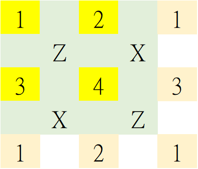
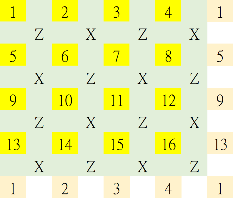
In the phenomenological noise model, achieving effective error correction with topological codes necessitates multiple rounds of syndrome extraction. In our simulations, we will focus on the family of rotated toric codes for even integers (as defined in [55, 56]). The lattices of the code for and are depicted in Fig. 5. Our experiments indicate that to achieve good decoding performance, up to rounds of syndrome extraction are required. Furthermore, the decoding performance starts to saturate even with more rounds of syndrome extraction, up to . We conjecture that this holds for general two-dimensional topological quantum codes.
We can reasonably assume that for a topological code with a minimum distance of , approximately rounds of repeated measurements are required. It is well-known that the minimum distance of a two-dimensional topological code grows as , where is the length of the code. Consequently, the generalized DS check matrix has error variables.
Similar to conventional BP, DS-(A)MBP has a worst-case time complexity of (cf. [41, 42]), where is the mean column weight of the check matrix, and is the maximum number of iterations, typically bounded by . In the case of a topological code, the mean column weight of its check matrix is roughly a constant, independent of the code length. Therefore, the complexity of DS-(A)MBP is .
We can compare the complexities of other decoders for reference. The RG decoder exhibits a complexity of as well. The MWPM has a complexity of , or when local matching is employed. These numbers are summarized in Table I.
V-B Simulations on toric codes
In this section, we conduct simulations on a quantum memory implemented with a code from a family of rotated toric codes for even integers . In this phenomenological noise model, we assume that the syndrome error rate and the data error rate are equal.
For BP decoding to be effective on the rotated toric codes, a non-parallel schedule and are required [42]. In the following, we will use the serial schedule (along variable nodes) for BP and set the maximum number of iterations . We will simulate DS-AMBP with .
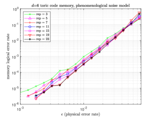
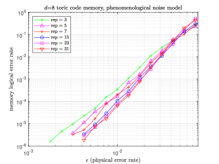
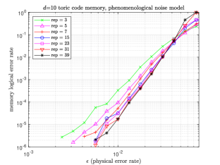
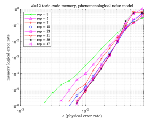
In Fig. 6, we show the performance of DS-AMBP in correcting quantum memories protected by the rotated toric codes with distances , respectively. The performance of each code is simulated for various rounds () of syndrome extractions, ranging up to . These are indicated by the term ‘rep’ in the legend for clarity.
As can be seen, under high physical error rates, smaller values of tend to yield better performance. This is because a high number of syndrome-extraction rounds can accumulate errors, potentially leading to uncorrectable logical errors. Conversely, when the physical error rate is sufficiently low, a larger number of rounds results in improved performance. As previously mentioned, it is suggested to perform approximately rounds of syndrome extraction. It is also evident that performance gains become less significant when exceeds . This reflects that, around , the error correction capabilities for syndrome errors and data errors begin to align.
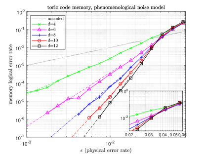
In Figure 7, performance curves are presented for the rotated toric codes with distances . Each curve for a code with distance is optimized across various rounds ranging from 3 to . To highlight the overall performance for each , one can utilize the lower envelope of the curves in each subfigure of Figure 6 as a representation of the optimized performance across different values.
Additionally, for each , a dashed curve is included as a reference curve, where , and is a scalar chosen to approximate the actual performance curve. The reference curves illustrate that the expected error correction capabilities for each specific are achieved using DS-AMBP.
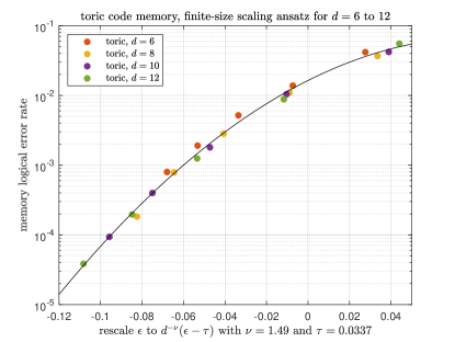
Next, we assess the error threshold for this family of phenomenological quantum memories using the finite-size scaling ansatz method [44]. To do so, we rescale to and replot Fig.7. We seek the optimal values of , with a precision of 0.1, and , with a precision of 0.0001, to fit a second-order curve with minimized mean squared error. The resulting values are and . The rescaled figure is presented in Fig. 8.
The value of provides an estimate of the error threshold for DS-AMBP on toric codes within the phenomenological noise model. The estimated error threshold is approximately 3.3%, which is close to the optimal threshold estimated in [46] (recovering RPGM), surpassing MWPM at 2.93% [44] and RG at 1.94% [60]. These results are summarized in Table I.
VI Single-shot quantum error correction
In this section, we focus on a special case of the phenomenological noise model involving only a single round of noisy syndrome extraction. This scenario is referred to as single-shot quantum error correction, and it becomes particularly important when the error rate of syndrome measurements is dominant over all other errors.
VI-A Design of low-overhead DS check matrix
In single-shot quantum error correction, it is common to measure redundant stabilizers to ensure that the syndromes are robust against measurement errors. By including an arbitrary number of stabilizers in the syndrome extraction, the impact of measurement errors can be minimized. However, since we are limited to a single round of syndrome extraction, it is reasonable to focus on a set of stabilizers that can be measured in parallel. Consequently, we assume only a small number of redundant stabilizers can be included in one round of syndrome extraction.
Let be a check matrix of a quantum code. Consider its DS check matrix
| (25) |
where and represents additional redundant stabilizers. After performing Gaussian elimination on this check matrix, we have
| (26) |
One may apply some row operations to and obtain a more general form by
| (27) |
where and may have .
For good BP decoding performance, Gallager suggested using a sparse check matrix with a mean column weight of at least 3 and a mean row weight of at least 4 [29]. In line with the idea of two-step decoding [22, 23], one might initially choose as an effective classical LDPC matrix such that has a mean column weight of 3. However, adhering to this design criterion could introduce an unnecessary surplus of redundant stabilizers.
Alternatively, we propose choosing to be a binary LDPC matrix with a mean column weight and a sufficiently large mean row weight so that . This is because we have a BP decoder for the whole check matrix, eliminating the need of a two-step decoding process. By choosing we conform to Gallager’s recommendation and minimize the number of additional redundant stabilizers in the matrix block . Moreover, the selection of an sufficiently large value of ensures a good classical distance [65, 29].
In the following proposition, we will demonstrate how to construct as a quasi-cyclic matrix, whose submatrices are circulant permutation matrices, derived from random permutations of the identity matrix [66]. This construction typically leads to an induced Tanner graph with sufficiently large girth (length of a shortest cycle), which, in turn, results in effective BP performance.
Proposition 1.
Consider the identity matrix , where is a chosen integer. Define matrix as
| (32) |
where each is a random circulant permutation matrix of . Then is a quasi-cyclic matrix with row weight and column weight . ∎
The parameters , , and can be chosen so that the number of additional redundant stabilizers is only a small fraction of .
VI-B Simulations on generalized bicycle codes
We consider the GB code in [38] with a check matrix. While this matrix already contains 28 redundant rows, it was not specifically designed for single-shot quantum error correction. Thus we remove 26 of these redundant rows, resulting in a quaternary check matrix over . In accordance with Proposition 1, we proceed to construct a quasi-cyclic matrix with parameters , , and . We perform this construction using heuristic random techniques and successfully create a matrix with a girth of 8. As a result, we obtain a DS check matrix with dimensions of in the form of Eq. (26).
Our error model assumes depolarizing errors with a rate of and syndrome bit flip errors with a rate of . To capture various scenarios, we will conduct simulations for the following cases:
(1) (perfect syndromes),
(2) ,
(3) , and
(4) .
This is reasonable because, in practical experiments, the measurement error rate can indeed be much worse than the other error gates [16, 17].
We perform simulations for these cases using DS-MBP with and DS-AMBP with . The maximum number of iterations is set to . The results are presented in Fig. 9. For comparison, we also include the bounded distance decoding (BDD) results for different combinations of and . The BDD decoding error rate is calculated using the formula:
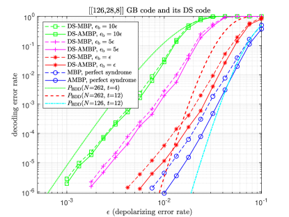
Since is assumed, the performance would be dominated by . Suppose that for and . Observing the DS-AMBP curves, we find that to achieve a decoding error rate below , the required physical error rate must be lower than 0.01, 0.0028, and 0.0014 for and respectively. These values are roughly proportional to .
Since the distance of the GB code is 8, there are some uncorrectable errors of weight four. We would like to have robust performance, particularly the ability to correct most errors of weight no larger than , even in scenarios with a high syndrome error rate, such as . This is achieved as shown in Fig. 9, where the DS-AMBP curve at falls below the BDD curve at .
Similarly, when , DS-(A)MBP can correct most errors of weight no larger than , and the performance relatively close to the case of perfect syndromes. In the case of , DS-(A)MBP still effectively corrects most errors with weight no larger than , demonstrating its robustness in scenarios with high syndrome errors during single-shot correction.
When the syndrome error rate is not dominant, such as in the cases of or , quantum degeneracy plays a significant role. An adaptive scheme like DS-AMBP or AMBP has an improved ability to identify degenerate errors on the data qubits, leading to enhanced performance [42].
For comparison, we created several examples by adding redundant stabilizers to the GB code, as follows:
-
•
Using Eq. (26) with , , and designed with , resulting in girth 8.
-
•
Using Eq. (27) with , , and designed with , resulting in girth 8.
-
•
Using Eq. (26) with , , and designed with , resulting in girth 6.
-
•
Using Eq. (27) with , , and designed with , resulting in girth 6.
We aimed to maximize the girth for each case. In our tests, the first case, which is our chosen approach, demonstrated the best performance. These results provide further support for our recommendation to construct a quasi-cyclic matrix with a mean column weight of
VII Conclusion
In this paper, we presented BP algorithms for decoding phenomenological errors with multiple rounds of syndrome extraction, extending the framework of DS codes. Our adaptive algorithm DS-AMBP demonstrated superior performance close to optimal threshold for phenomenological quantum memory protected by rotated toric codes compared to MWPM or RG decoders.
It is worth noting that there’s potential to reduce the required number of rounds for quantum memory through techniques like a sliding window [14].
In the phenomenological noise model, we made an interesting observation: the assumption of whether the final round of syndrome extraction is affected by data errors becomes less crucial, especially as the number of rounds increases.
We also delved into single-shot quantum error correction and proposed a DS check matrix construction with low overhead. Simulations showed the robust single-shot performance of DS-(A)MBP on the GB code, which we found to be applicable to many other codes as well.
As a future direction, we aim to generalize the techniques presented in this paper to address the circuit-level noise model, where each location in a quantum circuit might be faulty, and errors propagate through CNOT gates [67, 58]. This ongoing research will extend our understanding of quantum error correction.
Acknowledgment
KYK and CYL were supported by the National Science and Technology Council (NSTC) in Taiwan, under Grant 111-2628-E-A49-024-MY2, 112-2119-M-A49-007, and 112-2119-M-001-007.
References
- [1] C. H. Bennett and G. Brassard, “Quantum cryptography: Public key distribution and coin tossing,” in Proc. IEEE Int. Conf. Comput., Syst., Signal Process., 1984, pp. 175–179.
- [2] C. H. Bennett and S. J. Wiesner, “Communication via one- and two-particle operators on Einstein-Podolsky-Rosen states,” Phys. Rev. Lett., vol. 69, pp. 2881–2884, 1992.
- [3] C. H. Bennett, G. Brassard, C. Crepeau, R. Jozsa, A. Peres, and W. K. Wootters, “Teleporting an unknown quantum state via dual classical and Einstein-Podolsky-Rosen channels,” Phys. Rev. Lett., vol. 70, pp. 1895–1899, 1993.
- [4] P. W. Shor, “Algorithms for quantum computation: Discrete logarithms and factoring,” in Proc. Annu. Symp. Found. Comput. Sci. (FOCS), 1994, pp. 124–134.
- [5] L. K. Grover, “A fast quantum mechanical algorithm for database search,” in Proc. Annu. ACM Symp. Theory Comput. (STOC), 1996, pp. 212–219.
- [6] J. I. Cirac, P. Zoller, H. J. Kimble, and H. Mabuchi, “Quantum state transfer and entanglement distribution among distant nodes in a quantum network,” Phys. Rev. Lett., vol. 78, p. 3221, 1997.
- [7] H.-J. Briegel, W. Dür, J. I. Cirac, and P. Zoller, “Quantum repeaters: the role of imperfect local operations in quantum communication,” Phys. Rev. Lett., vol. 81, p. 5932, 1998.
- [8] E. Farhi, J. Goldstone, and S. Gutmann, “A quantum approximate optimization algorithm,” 2014, e-print at https://arxiv.org/abs/1411.4028.
- [9] A. Peruzzo, J. McClean, P. Shadbolt, M.-H. Yung, X.-Q. Zhou, P. J. Love, A. Aspuru-Guzik, and J. L. O’brien, “A variational eigenvalue solver on a photonic quantum processor,” Nat. Commun., vol. 5, pp. 1–7, 2014.
- [10] P. W. Shor, “Fault-tolerant quantum computation,” in Proc. Annu. Conf. Found. Comput. Sci. (FOCS), 1996, pp. 56–65.
- [11] D. Gottesman, “Stabilizer codes and quantum error correction,” Ph.D. dissertation, Caltech. e-print at https://doi.org/10.7907/rzr7-dt72, 1997.
- [12] A. R. Calderbank, E. M. Rains, P. W. Shor, and N. J. A. Sloane, “Quantum error correction via codes over GF(4),” IEEE Trans. Inf. Theory, vol. 44, pp. 1369–1387, 1998.
- [13] M. A. Nielsen and I. L. Chuang, Quantum Computation and Quantum Information. Cambridge University Press, 2000.
- [14] E. Dennis, A. Kitaev, A. Landahl, and J. Preskill, “Topological quantum memory,” J. Math. Phys., vol. 43, pp. 4452–4505, 2002.
- [15] D. J. C. MacKay, G. Mitchison, and P. L. McFadden, “Sparse-graph codes for quantum error correction,” IEEE Trans. Inf. Theory, vol. 50, pp. 2315–2330, 2004.
- [16] F. Arute, K. Arya, R. Babbush, D. Bacon, J. C. Bardin et al., “Quantum supremacy using a programmable superconducting processor,” Nature, vol. 574, pp. 505–510, 2019.
- [17] Y. Chen, M. Farahzad, S. Yoo, and T.-C. Wei, “Detector tomography on IBM quantum computers and mitigation of an imperfect measurement,” Phys. Rev. A, vol. 100, p. 052315, 2019.
- [18] C. Ryan-Anderson, J. G. Bohnet, K. Lee, D. Gresh, A. Hankin, J. Gaebler, D. Francois, A. Chernoguzov, D. Lucchetti, N. C. Brown et al., “Realization of real-time fault-tolerant quantum error correction,” Phys. Rev. X, vol. 11, p. 041058, 2021.
- [19] M. Abobeih, Y. Wang, J. Randall, S. Loenen, C. Bradley, M. Markham, D. Twitchen, B. Terhal, and T. Taminiau, “Fault-tolerant operation of a logical qubit in a diamond quantum processor,” Nature, vol. 606, pp. 884–889, 2022.
- [20] S. Krinner, N. Lacroix, A. Remm, A. Di Paolo, E. Genois, C. Leroux, C. Hellings, S. Lazar, F. Swiadek, J. Herrmann et al., “Realizing repeated quantum error correction in a distance-three surface code,” Nature, vol. 605, pp. 669–674, 2022.
- [21] Y. Kim, A. Eddins, S. Anand, K. X. Wei, E. van den Berg, S. Rosenblatt, H. Nayfeh, Y. Wu, M. Zaletel, K. Temme, and A. Kandala, “Evidence for the utility of quantum computing before fault tolerance,” Nature, vol. 618, pp. 500–505, 2023.
- [22] A. Ashikhmin, C.-Y. Lai, and T. A. Brun, “Robust quantum error syndrome extraction by classical coding,” in Proc. IEEE Int. Symp. Inf. Theory (ISIT), 2014, pp. 546–550.
- [23] ——, “Correction of data and syndrome errors by stabilizer codes,” in Proc. IEEE Int. Symp. Inf. Theory (ISIT), 2016, pp. 2274–2278.
- [24] ——, “Quantum data-syndrome codes,” IEEE J. Sel. Areas Commun., vol. 38, pp. 449–462, 2020.
- [25] Y. Fujiwara, “Ability of stabilizer quantum error correction to protect itself from its own imperfection,” Phys. Rev. A, vol. 90, p. 062304, 2014.
- [26] H. Bombín, “Single-shot fault-tolerant quantum error correction,” Phys. Rev. X, vol. 5, p. 031043, 2015.
- [27] E. T. Campbell, “A theory of single-shot error correction for adversarial noise,” Quantum Sci. Technol., vol. 4, p. 025006, 2019.
- [28] N. Delfosse, B. W. Reichardt, and K. M. Svore, “Beyond single-shot fault-tolerant quantum error correction,” IEEE Trans. Inf. Theory, vol. 68, pp. 287–301, 2022.
- [29] R. G. Gallager, Low-Density Parity-Check Codes, ser. no. 21 in Research Monograph Series. MIT Press, 1963.
- [30] D. J. C. MacKay and R. M. Neal, “Near Shannon limit performance of low density parity check codes,” Electronics Letters, vol. 32, pp. 1645–1646, 1996.
- [31] D. J. C. MacKay, “Good error-correcting codes based on very sparse matrices,” IEEE Trans. Inf. Theory, vol. 45, pp. 399–431, 1999.
- [32] R. Tanner, “A recursive approach to low complexity codes,” IEEE Trans. Inf. Theory, vol. 27, pp. 533–547, 1981.
- [33] J. Pearl, Probabilistic reasoning in intelligent systems: networks of plausible inference. Kaufmann, 1988.
- [34] F. R. Kschischang, B. J. Frey, and H.-A. Loeliger, “Factor graphs and the sum-product algorithm,” IEEE Trans. Inf. Theory, vol. 47, pp. 498–519, 2001.
- [35] D. Poulin and Y. Chung, “On the iterative decoding of sparse quantum codes,” Quantum Inf. Comput., vol. 8, pp. 987–1000, 2008.
- [36] Y.-J. Wang, B. C. Sanders, B.-M. Bai, and X.-M. Wang, “Enhanced feedback iterative decoding of sparse quantum codes,” IEEE Trans. Inf. Theory, vol. 58, pp. 1231–1241, 2012.
- [37] Z. Babar, P. Botsinis, D. Alanis, S. X. Ng, and L. Hanzo, “Fifteen years of quantum LDPC coding and improved decoding strategies,” IEEE Access, vol. 3, pp. 2492–2519, 2015.
- [38] P. Panteleev and G. Kalachev, “Degenerate quantum LDPC codes with good finite length performance,” Quantum, vol. 5, p. 585, 2021.
- [39] J. Roffe, D. R. White, S. Burton, and E. T. Campbell, “Decoding across the quantum LDPC code landscape,” Phys. Rev. Res., vol. 2, p. 043423, 2020.
- [40] K.-Y. Kuo and C.-Y. Lai, “Refined belief propagation decoding of sparse-graph quantum codes,” IEEE J. Sel. Areas Inf. Theory, vol. 1, pp. 487–498, 2020.
- [41] C.-Y. Lai and K.-Y. Kuo, “Log-domain decoding of quantum LDPC codes over binary finite fields,” IEEE Trans. Quantum Eng., vol. 2, 2021, article no. 2103615.
- [42] K.-Y. Kuo and C.-Y. Lai, “Exploiting degeneracy in belief propagation decoding of quantum codes,” npj Quantum Inf., vol. 8, 2022, article no. 111. (See a complete version at https://arxiv.org/abs/2104.13659).
- [43] ——, “Comparison of 2D topological codes and their decoding performances,” in Proc. IEEE Int. Symp. Inf. Theory (ISIT), 2022, pp. 186–191.
- [44] C. Wang, J. Harrington, and J. Preskill, “Confinement-Higgs transition in a disordered gauge theory and the accuracy threshold for quantum memory,” Ann. Phys., vol. 303, pp. 31–58, 2003.
- [45] J. W. Harrington, “Analysis of quantum error-correcting codes: symplectic lattice codes and toric codes,” Ph.D. dissertation, Caltech, 2004.
- [46] T. Ohno, G. Arakawa, I. Ichinose, and T. Matsui, “Phase structure of the random-plaquette gauge model: accuracy threshold for a toric quantum memory,” Nucl. Phys. B, vol. 697, pp. 462–480, 2004.
- [47] B. M. Terhal, “Quantum error correction for quantum memories,” Rev. Mod. Phys., vol. 87, p. 307, 2015.
- [48] J.-P. Tillich and G. Zémor, “Quantum LDPC codes with positive rate and minimum distance proportional to the square root of the blocklength,” IEEE Trans. Inf. Theory, vol. 60, pp. 1193–1202, 2014.
- [49] A. A. Kovalev and L. P. Pryadko, “Quantum Kronecker sum-product low-density parity-check codes with finite rate,” Phys. Rev. A, vol. 88, p. 012311, 2013.
- [50] S. Bravyi and M. B. Hastings, “Homological product codes,” in Proc. Annu. ACM Symp. Theory Comput. (STOC), 2014, pp. 273–282.
- [51] A. Leverrier, J.-P. Tillich, and G. Zémor, “Quantum expander codes,” in Proc. Annu. Symp. Found. Comput. Sci. (FOCS), 2015, pp. 810–824.
- [52] P. Panteleev and G. Kalachev, “Quantum LDPC codes with almost linear minimum distance,” IEEE Transactions on Information Theory, vol. 68, no. 1, pp. 213–229, 2022.
- [53] A. Y. Kitaev, “Fault-tolerant quantum computation by anyons,” Ann. Phys., vol. 303, pp. 2–30, 2003, arXiv preprint quant-ph/9707021.
- [54] H. Bombin and M. A. Martin-Delgado, “Topological quantum distillation,” Phys. Rev. Lett., vol. 97, p. 180501, 2006.
- [55] ——, “Optimal resources for topological two-dimensional stabilizer codes: Comparative study,” Phys. Rev. A, vol. 76, p. 012305, 2007.
- [56] C. Horsman, A. G. Fowler, S. Devitt, and R. Van Meter, “Surface code quantum computing by lattice surgery,” New J. Phys., vol. 14, p. 123011, 2012.
- [57] J. Edmonds, “Paths, trees, and flowers,” Can. J. Math., vol. 17, pp. 449–467, 1965.
- [58] D. S. Wang, A. G. Fowler, A. M. Stephens, and L. C. L. Hollenberg, “Threshold error rates for the toric and planar codes,” Quantum Inf. Comput., vol. 10, pp. 456–469, 2010.
- [59] G. Duclos-Cianci and D. Poulin, “Fast decoders for topological quantum codes,” Phys. Rev. Lett., vol. 104, p. 050504, 2010.
- [60] ——, “Fault-tolerant renormalization group decoder for abelian topological codes,” Quantum Inf. Comput., vol. 14, pp. 721–740, 2014.
- [61] K.-Y. Kuo, I.-C. Chern, and C.-Y. Lai, “Decoding of quantum data-syndrome codes via belief propagation,” in Proc. IEEE Int. Symp. Inf. Theory (ISIT), 2021, pp. 1552–1557.
- [62] E. Knill and R. Laflamme, “A theory of quantum error-correcting codes,” Phys. Rev. A, vol. 55, no. 2, pp. 900–911, 1997.
- [63] K.-Y. Kuo and C.-C. Lu, “On the hardnesses of several quantum decoding problems,” Quantum Inf. Process., vol. 19, pp. 1–17, 2020.
- [64] P. Iyer and D. Poulin, “Hardness of decoding quantum stabilizer codes,” IEEE Trans. Inf. Theory, vol. 61, pp. 5209–5223, 2015.
- [65] F. J. MacWilliams and N. J. A. Sloane, The Theory of Error-Correcting Codes. North-Holland Publishing Company, 1977.
- [66] M. P. C. Fossorier, “Quasi-cyclic low-density parity-check codes from circulant permutation matrices,” IEEE Trans. Inf. Theory, vol. 50, pp. 1788–1793, 2004.
- [67] R. Raussendorf, J. Harrington, and K. Goyal, “Topological fault-tolerance in cluster state quantum computation,” New J. Phys., vol. 9, p. 199, 2007.
We show that the calculations in Algorithm 2 with provide an approximation to the solution based on the given syndrome. We will provide a justification for the first iteration, and subsequent iterations will further improve the approximation as the beliefs are propagated throughout the Tanner graph.
The choice of the normalization parameter and the fixed inhibition is tailored to achieve good performance with degenerate codes. For a more in-depth discussion on this aspect, please refer to [42].
Consider a generalized check matrix of the form
where and .
Assume that we have an error vector , where ’s and ’s are independently draw according to the distributions for each and for each .
An approximation to the distribution of , conditioned on a given syndrome vector , is the product of the conditional marginal distributions of ’s and ’s. Thus we would like to approximately compute the following LLRs
| (33) | |||
| (34) |
We derive the update procedure for obtaining in the following. Obtaining would be similar.
We have the following initial LLRs according to the channel statistics:
| (35) | ||||
| (36) |
Recall that we have the sets of neighboring nodes for check node and for variable node . Note that is the support of row in . Let be the restriction of to , and let denote the -th row of . Then the error syndrome relations can be written as for . For a fixed , if it participates in check ,
| (37) |
where means to simplify the notation. For convenience, consider an event for some that satisfies the syndrome. Then (37) can be written as
| (38) |
if , or
| (39) |
if for . These two equations will be used later.
By Bayes rule,
| (40) |
The term can be computed as follows:
| (41) | ||||
| (42) | ||||
| (43) |
Since
we have
| (44) | ||||
| (45) |
where
| (46) |
The symbol represents a proportional approximation and this approximation is particularly effective when dealing with sparse check matrices.
A similar approach is applied to obtain a form similar to (45) for approximating by using equation (38).
To simplify the notation, we introduce a mixed-alphabet representation of the event:
| (47) |
where and . Then (46) can be written as
| (48) |
With , we define two conditions to be used later
| (49) | |||
| (50) |
When the Tanner graph is a tree, the proportional approximation in (45) becomes an equality after the beliefs are passed. As mentioned, this approximation typically holds well for sparse check matrices. As a result, we adopt the following update rule by substituting the outcomes from (44)–(48) back into (40):
| (51) |
where the summation term can be simplified as
| (52) |
Recall that if the alphabet is quaternary, we compute a scalar message using as in (21). Notice that
| (53) | |||
| (54) |
We extend this function to mixed alphabets:
| (55) |
where for and for . Then the update rule mentioned in (51)–(52) can be efficiently computed by using the operator in (22):
| (56) |
This can be proved by induction. The procedure is straightforward and similar to that in [41, Appendix A]. We omit this part for brevity.
For binary variables, can be computed similarly as
| (57) |