Weakly Supervised Learning for Breast Cancer Prediction on Mammograms in Realistic Settings

Abstract

Automatic methods for early detection of breast cancer on mammography can significantly decrease mortality. Broad uptake of those methods in hospitals is currently hindered because the methods have too many constraints. They assume annotations available for single images or even regions-of-interest (ROIs), and a fixed number of images per patient. Both assumptions do not hold in a general hospital setting. Relaxing those assumptions results in a weakly supervised learning setting, where labels are available per case, but not for individual images or ROIs. Not all images taken for a patient contain malignant regions and the malignant ROIs cover only a tiny part of an image, whereas most image regions represent benign tissue. In this work, we investigate a two-level multi-instance learning (MIL) approach for case-level breast cancer prediction on two public datasets (1.6k and 5k cases) and an in-house dataset of 21k cases. Observing that breast cancer is usually only present in one side, while images of both breasts are taken as a precaution, we propose a domain-specific MIL pooling variant. We show that two-level MIL can be applied in realistic clinical settings where only case labels, and a variable number of images per patient are available. Data in realistic settings scales with continuous patient intake, while manual annotation efforts do not. Hence, research should focus in particular on unsupervised ROI extraction, in order to improve breast cancer prediction for all patients.

Case-level breast cancer prediction, deep neural network, mammography images, multi-instance learning, weakly supervised learning.

1 Introduction

Breast cancer is the most common cancer with 2.26 million cases reported worldwide in 2020 causing 685k deaths [1]. Early detection of breast cancer using mammography as diagnostic test has led to a significant decrease in breast cancer mortality [2, 3]. Automatic breast cancer detection methods on mammography improve clinical tools and reduce radiologists’ workload [4, 5, 6]. Those automatic methods are usually trained in a fully supervised manner with labels available at the image-level [7, 8] or even at the region-of-interest (ROI) level [9, 4]. Such annotations, however, are not available in a standard clinical workflow, and their acquisition is not feasible due to high costs and time demands from clinicians. In a standard clinical workflow, groundtruth is only available for a mammography case, containing multiple images from both breast sides. That is, breast cancer prediction in a realistic setting is a weakly supervised learning task with three particular challenges:

1. Groundtruth is only available for a case, and not for individual images (cf. Table 3, Label in MGM).

2. ROIs are not annotated and abnormalities cover only 2% of the image regions [10].

3. A mammography examination can result in a variable number of images per case (cf. Table 3 Case Dist.).

Neither of the current approaches addresses all three challenges. Approaches that rely on annotated datasets with ROI [11, 4], image [12, 7] or side [13, 14] labels are not applicable to datasets with case-level labels (C1, C2). Assigning case labels to all images in a case [6, 14] creates noisy datasets since malignancies are not necessarily visible in all images (C1). Similarly, creating models that average image labels for case-level prediction [15] does not account for malignancies only visible in single images (C1), and might result in low performance for highly imbalanced cases. Approaches that concatenate feature representations over views to create a case-level representation [5, 16] or fix the number of views by excluding images [15, 5] can not handle a variable number of images per case (C3). Approaches that apply weakly supervised learning at the image-level for unsupervised extraction of ROIs [8, 17] address C2, but assume availability of image labels (C1). Further, approaches that use multiscale, multiresolution features of images for better detection of ROIs, assume ROI annotations [18] or breast side labels [13] for training (C1, C2).

Table 1: Comparison of our work to existing state-of-the-art in breast cancer prediction with mammography. Instances report the number of ROIs (R)/ images (I)/ cases (C) in the dataset, task shows the classification problem - malignant (M), benign (B), normal (N), abnormal (A = M+B). Views states the number of images the model takes as input, e.g. 4 indicates LCC, LMLO, RCC, RMLO. ROI annotation used in training (✓) vs not (✗). Level indicates the input level for training and prediction. ^∗AUC on CBIS taken from [7], ^†uses hand-crafted features, ^‡our reproduction. Works differ in data, reporting standard, label.

Paper	Year	Dataset	Instances	Task	Abnormality	Views	ROI	Level	AUC
Rampun et al. [9]	2018	CBIS	1,593 (R)	M/B	mass	1	✓	ROI	0.84
Tsochatzidis et al.[19]	2019	CBIS	1,697 (R)	M/B	mass	1	✓	ROI	0.80
Ragab et al. [20]	2021	CBIS	5,272 (R)	M/B	mass	1	✓	ROI	1.00
Khan et al.[21]	2019	MIAS-CBIS	3,890 (R)	M/B	mass, calc	4	✓	ROI-Case	0.77
Zhu et al. [12]	2017	CBIS	1,644 (C)	M/B	mass, calc.	1	✗	Image	0.79∗
Shen et al. [4]	2019	CBIS	2,478 (I)	M/B	mass, calc.	1	✓	Image	0.88
Shu et al. [7]	2020	CBIS	3,071 (I)	M/B	mass, calc.	1	✗	Image	0.84
Shen et al. [8]	2021	CBIS	1,644 (C)	M/B	mass, calc.	1	✗	Image	0.86
Wei et al. [22]	2022	CBIS	3,103 (I)	M/B	mass, calc.	1	✗	Image	0.83
Carneiro et al. [16]	2015	DDSM	680 (I)	M/B	mass, calc.	2	✓	Breast side	0.97
Akselrod et al.[14]	2019	Private	52,936 (I)	M/rest	all	4	✗	Breast side	0.91
Wu et al. [5]	2020	Private	229,426 (C)	M/B/N	all	4	✓	Breast side	0.89
Petrini et al. [23]	2022	CBIS	2,694 (I)	M/B	mass, calc.	2	✓	Breast side	0.85
Quellec et al. [24]	2016	DDSM	2,479 (C)	A/N	mass, calc.	4	✗	Case	0.80†
Kim et al. [15]	2018	Private	29,107 (C)	M/N	all	4	✗	Case	0.91
		CBIS	1,645 (I)	M/B	mass, calc.	Any	✗	Case	0.64‡
McKinney et al. [25]	2020	OPTIMAM	102,640 (C)	M/rest	all	4	✓	Case	0.89
This work	2023	CBIS	1,645 (C)	M/B	mass, calc.	Any	✗	Case	0.79
		VinDr	5,000 (C)	M/rest	all	Any	✗	Case	0.83
		Private	21,013 (C)	M/rest	all	Any	✗	Case	0.85

Multi-Instance Learning (MIL) [26] is promising for our weakly supervised learning task, as MIL learns from labelled bags of instances, without labels for individual instances. In our setting, the bag is the labelled case and images are the unlabelled instances. We pose breast cancer prediction in realistic settings as a MIL task on two levels: on image-level, not all images correspond to the bag label (C1) and on patch-level, most regions of the image do not correspond to the image label (C2). Most similar to our work, Quellec et al. [24] extract image regions, calculate hand-crafted features from the extracted regions and apply standard MIL approaches [27, 28, 26, 29] at the case-level. However, their hand-crafted features require heavy hyper-parameter tuning already at region extraction. Instead, we aim for end-to-end learning that is suitable for a variety of realistic breast cancer prediction settings on mammography cases. In particular, we aim for a method that assumes only case-level labels, accounts for malignancies present only in a subset of images per case and in small regions of those images, and is able to handle a variable number of images per case (C1, C2, C3).

The contributions of our paper are as follows:

1. We describe a realistic setting for breast cancer prediction on mammography through a hospital dataset with case labels and variable images across cases (cf. Table 3 MGM).

2. We present a case-level MIL model that is capable of handling a variable number of images, has unsupervised ROI extraction and a novel domain-specific side-wise MIL pooling at the image-level (cf. Fig. 1). We obtain competitive performance on the two benchmark datasets CBIS (AUC 0.81) and VinDr (AUC 0.83), and on our private dataset, MGM (AUC 0.85).

3. We show that MIL model trained on case labels only, achieves similar performance to models trained on image labels, suggesting that case labels are sufficient and image-level annotation is not necessary (Table 5).

For reproducibility, we publish our code and training details.

Terminology. A mammography is the diagnostic test, a mammogram (or image) refers to an X-ray image captured during mammography. A case refers to the set of images taken for a patient during mammography. A case consists of at most 1 image of type $side_{k}view_{i}$. A $view_{i}\in$ {craniocaudal (CC), mediolateral oblique (MLO), lateromedial (LM), mediolateral (ML), exaggerated craniocaudal (XCCL)} captures different angles of the breast $side_{k}\in$ {left (L), right (R)}. CC and MLO are the standard views taken during mammography, with other additional views taken to rule out or confirm abnormalities. Variable-images refer to the non-fixed number of images per case, including variable-views.

2 State of the Art and Reproducibility

In this section we review state-of-the-art (SoTA) models on breast cancer prediction and conduct experiments to identify the most promising feature extraction method.

2.1 Comparison of SoTA Models

Table 1 summarizes SoTA methods for breast cancer prediction using mammography. To highlight differences across methods, we report the dataset used, the number of instances and the abnormalities included in the dataset (e.g. mass, calcification, or all). We also report the classification task, number of views accepted as input, whether ROI annotations are used during training, the level at which the prediction is done (also same as the training label), e.g., ROI, image, breast side or case level and the AUC score.

We found that the reported scores cannot be compared, because datasets differ and not all papers use a publicly available dataset, e.g., CBIS-DDSM (CBIS) [30], DDSM [31], VinDr [32] or MIAS-CBIS, a combination of MIAS and CBIS. Even methods that report results on the same public datasets (e.g., CBIS) differ in i) their data, ii) the reporting standards of the result, and iii) the input level for training and prediction. Methods differ in data due to the addition of instances over time [7, 22], restriction to a specific abnormality [19, 9], increase in the training dataset by data augmentation [11, 20], and use of custom dataset split [4]. [22] reported a difference of 13% in AUC for [4] on official split (AUC 0.75) vs custom split (AUC 0.88) of CBIS. The reporting standards of results differ due to use of test time augmentation to report final scores (improves the performance by 1-2% [22]) and use of model ensembles [8, 22]. Further, methods differ in training label and prediction level, e.g., training with ROI labels for prediction at the ROI-level [11, 9, 19], image-level [4, 33, 34], side-level [5, 23], and case-level [25]; training with image labels for image-level predictions [12, 7, 8, 35]; training with breast side label for side-level predictions [5, 16, 14]. Some methods also use fine-grained labels that are hard to obtain in practice to train classifiers on detailed classes, e.g., abnormality type [4, 6]. We color coded the AUC scores to indicate how comparable the scores are to our result: lightgray indicates differences in the dataset or CBIS split, darkgray indicates results reported on the official CBIS split, but differ in reporting standards or training label used, black is fully comparable results on official CBIS split.

Based on our analysis, we shortlisted two unsupervised ROI extraction methods [7, 8] as image-level feature extractor for our MIL model. We also shortlisted the feature extractor of Kim et al. [15] as it is the strongest case-level baseline. We implemented and compared them to select the best feature extractor for our case-level MIL model.

2.2 Reproducibility and Choice of Feature Extractor

Since source code is not available for any of the selected candidates (except GMIC [8], which has only inference code available), we reproduced related work from the information given in the corresponding paper. We publish our implementation of these methods along with the training details.¹ We compared global feature learning models trained from scratch against pretrained models. Specifically, we compared DIB-MG [15], an adapted single channel ResNet model trained from scratch with a fine-tuned pretrained DenseNet169 with global average pooling (avgpool) or max pooling (maxpool) in the last layer before the classification head [7] and a pretrained Resnet34 with avgpool [8]. We also compared global feature learning models with unsupervised ROI candidates extraction methods, specifically a pretrained DenseNet169 with region-based group max pooling (RGP) and global group-max pooling (GGP) [7], and GMIC-ResNet18 [8]. We report performance (cf. Table 2) as stated in the original papers and from our reproduction on the official split of CBIS for image-level prediction, i.e., a model takes as input a mammogram image and is trained with the image label.

Similar to previous work [36], we observed that results reported by the original authors differ from our reproduction, i.e., we observe smaller performance values. We confirm previous findings that models with pretrained computer vision backbones (DenseNet169, Resnet34) outperform backbones trained from scratch (DIB-MG) [16, 11, 19]. The unsupervised ROI extraction model, GMIC-ResNet18, is on par with a standard Resnet34, and outperforms the other unsupervised ROI extraction methods RGP and GGP by $0.04$ points in F1 score. For our further experiments, we selected GMIC-ResNet18 as the feature extractor for our case-level models.

Table 2: Comparing feature-extractors for image-level prediction on official CBIS split. Batch size set to 10.

Model	F1${}^{\textit{Our}}$	AUC${}^{\textit{Our}}$	AUC${}^{\textit{Paper}}$
DIB-MG[15]	$0.54\pm 0.02$	$0.64\pm 0.00$	n.a.
DenseNet169 [7]
+ avgpool	$0.62\pm 0.03$	$0.76\pm 0.01$	$0.76\pm 0.00$
+ maxpool	$0.63\pm 0.01$	$0.74\pm 0.00$	$0.74\pm 0.00$
+ RGP (k=0.7)	$0.62\pm 0.01$	$0.76\pm 0.01$	${0.84}\pm 0.00$
+ GGP (k=0.7)	$0.62\pm 0.03$	$0.76\pm 0.02$	$0.82\pm 0.00$
Resnet34 [8]	$\textbf{0.66}\pm 0.02$	$0.78\pm 0.01$	$0.79\pm 0.01$
GMIC-ResNet18 [8]	$\textbf{0.66}\pm 0.02$	$\textbf{0.79}\pm 0.02$	$0.83\pm 0.00$

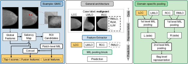
Figure 1: Model architecture. Center: overall architecture. An end-to-end trained feature extractor is applied to a variable number of input images (e.g. LCC, LMLO, RCC), returning a feature representation per image. Multi-instance learning (MIL) methods then aggregate these feature for a final decision. We compare different MIL pooling methods in our experiments. Left: An example feature extractor module, GMIC, capable of unsupervised ROI extraction. Right: Our domain-specific pooling block attending on single images and additionally incorporating features for each side (based on the assumption that single images of one side highly correlate in their cancerous state). Dashed lines indicate absent views. Best viewed in color.

3 Approach

Our task is to predict the classes malignant or benign given a mammogram case containing any number of views from breast sides (left, right). In the single-instance learning (SIL) setting, the model learns the class label $Y\in\{0,1\}$ ($0$: benign, $1$: malignant) based on one input instance, i.e., one image. In the MIL setting, classification is performed on a bag of instances, $X=\{x_{1},x_{2},..,x_{K}\}$ with a bag label $\in\{0,1\}$. The instances in the bag have no ordering and no relation among each other (i.e., the bag is a set of instances). Each instance in the bag has a label, $y_{k}$, which remains unknown while only the label of the bag is known. In binary MIL, a bag is considered positive if it contains at least one positive instance [26]. Similarly, if a mammogram case (bag) contains at least one malignant image (instance), the case is considered malignant, otherwise benign. The MIL model framework is shown in Fig. 1 center. Each mammogram image in a case is passed to a feature extractor module shared among all images. The feature representations are passed to the image-level MIL pooling block to generate the bag-level prediction. For image-level MIL pooling, we investigated pooling in instance and in embedded space. Our framework is feature extractor agnostic.

3.1 Feature Extractor

We use GMIC-ResNet18 (referred as GMIC) [8] as feature extractor (see Section 2.2 for a comparison of feature extractors). GMIC takes a mammogram image as input (cf. Fig. 1 left), learns global level features using ResNet18 [37], which are then passed through a 1$\times$1 convolution and sigmoid to generate a class-specific saliency map, encoding the malignant probability for all regions. The top $t$ scores from this saliency map are called Top-t features. The saliency map is then used to retrieve the top-k ROI candidates (patches) from the original image. Each patch is passed through another ResNet18 feature extractor and the last layer feature representation of all patches is aggregated with Gated Attention (patch-level MIL) [38], generating local features. The global features and local features are concatenated into fusion features.

3.2 MIL Pooling Block

Our image-level MIL task is to predict the label for a case without knowing the image labels. In MIL, image information can be aggregated on score (instance-space (IS)) [27] or feature (embedded-space (ES)) [39, 40] level using different aggregation strategies (MIL pooling). In IS MIL, the model outputs class scores for each instance, which are aggregated using MIL pooling to output a bag-level score. Different MIL pooling functions correspond to different assumptions in IS [41, 42]. Max pooling assumes that every positive bag has at least one positive instance, which is selected for the bag-level decision (standard multi-instance assumption). Mean pooling averages logits and assumes that every instance contributes equally to the bag-level decision (collective assumption), while attention pooling is used to weigh output scores if contribution of instances differ and have to be learned (weighted collective assumption). In ES MIL, the information is aggregated at the feature embedding level, and mapped to a bag-level feature vector using similar aggregation strategies.

We used the following four MIL pooling functions: mean, max [43], attention (Att), and gated-attention (GAtt) [38] defined as follows. Let $x_{k}$ be an input instance $k$ from bag $X$ containing $K$ instances, $f$ be the feature embedding function of a feature extractor and $g$ be the classification function. Further, let $m_{k}$ be the input to the MIL pooling function $\rho$. For IS, $m_{k}$ is the class logit $l_{k}$, for ES paradigm $m_{k}$ is the feature embedding $h_{k}$. Let $S$ be the bag-level logits for the classes. The MIL pooling operations for IS and ES can be written as:

IS: $$m_{k}=l_{k}=g(f(x_{k})),\> S=\rho(m_{k})$$

ES: $$m_{k}=h_{k}=f(x_{k}),\> S=g(\rho(m_{k}))$$

with the following pooling operations $\rho(m_{k})$:

$$\rho_{\text{Mean}}=\frac{1}{K}\sum_{k=1}^{K}m_{k},\;\rho_{\text{Max}}=\max_{k}m_{k},\;\rho_{\text{(G)Att}}=\sum_{k=1}^{K}a_{k}m_{k}$$

The attention weights $a_{k}$ definitions differ for Att and GAtt:

$$a_{k}^{\text{Att}} =\frac{\exp\{\mathbf{w}^{\top}\tanh(\mathbf{V}\mathbf{h}_{k}^{\top})\}}{\sum_{j=1}^{K}\exp\{\mathbf{w}^{\top}\tanh(\mathbf{V}\mathbf{h}_{j}^{\top})\}}$$

$$a_{k}^{\text{GAtt}} =\frac{\exp\{\mathbf{w}^{\top}(\tanh(\mathbf{V}\mathbf{h}_{k}^{\top})\odot\text{sigm}(\mathbf{U}\mathbf{h_{k}}^{\top}))\}}{\sum_{j=1}^{K}\exp\{\mathbf{w}^{\top}(\tanh(\mathbf{V}\mathbf{h}_{j}^{\top})\odot\text{sigm}(\mathbf{U}\mathbf{h_{j}}^{\top}))\}},$$

$\mathbf{w},\mathbf{V},\mathbf{U}$ are trainable parameters, $\tanh$, sigm (sigmoid) are activation functions, $\odot$ is element-wise multiplication.

For MIL pooling on GMIC features, we performed MIL pooling individually on the three types of features: top-t features, local features and fusion features (cf. Fig. 1). For IS, we mapped the three image-level features to three separate image-level scores and then applied MIL to obtain three case-level scores. For ES, we applied the MIL pooling separately on the three image-level feature embeddings to create three case-level features. For both IS and ES, top-t features were mapped to a score by averaging, whereas fusion features and local features were mapped to a score using a FC layer. The MIL pooling and the feature extractor module were trained together using the case labels as target.

3.3 Domain-specific MIL Pooling Block

In standard MIL, all instances of a bag are conceptually equal, resulting in image-wise aggregation of the feature embedding (image-wise pooling ^img). A mammography case, however, typically contains images of both breast sides (left and right). Malignancies can either not occur, occur on one side or on both sides. To find and weigh the condition of each side separately for creating the aggregated bag-level feature embedding, we propose a domain-specific pooling block for side-wise aggregation in embedded space (side-wise pooling ^side). Feature embeddings are combined separately per side with MIL pooling attention, and the resulting left and right feature embedding are combined by another MIL pooling attention operation (cf. Fig. 1, right). We used distinct attention modules for each level.

3.4 Variable-Image Handling in MIL Models

In a realistic scenario, a variable number of images is available per patient. MIL is inherently capable of handling variable bag sizes. However, it fails to be so due to the way pytorch implements keeping track of past updates for optimizers such as Adam [44]. Even if a component is not present in the forward pass and hence should not change, the parameters are still updated via the gradient history. This affects in particular the (gated) attention modules, which for example do not need to be updated when only a single image is present in the bag. We use a dynamic training approach for our MIL models to handle any number of input images without such undesired parameter updates. We group training batches by same combination of image types, e.g., LCC+LMLO in one batch, LCC+RCC+RMLO in another. After each mini-batch weight update, we reset the weights and the optimizer state of the unused components to the last state, where weights were updated directly from the input and gradient history and not from the gradient history alone.

4 Experimental Setup

In this section, we describe the datasets and their preprocessing, settings for model training, and evaluation. Our retrospective study was approved by the institutional review board of Hospital Group Twente (ZGT), The Netherlands.

4.1 Datasets

We evaluate our method on two public benchmarks - CBIS-DDSM (1.6k cases), VinDr (5k cases) and our in-house dataset MGM (21k cases). Table 3 shows an overview of all datasets.

CBIS-DDSM (CBIS) [30] is a public dataset comprising 3,103 mammograms from 1,566 patients including only CC and MLO views. It contains manually extracted ROI with groundtruth labels at ROI-level. We transferred the ROI-level labels to image-level by assigning malignant when any ROI (lesion) in the image has the label malignant, otherwise we label the image as benign (R$\rightarrow$I). Further, we created case-level labels inferred from the image labels with the groundtruth of a case as malignant if any image in a case is malignant, otherwise benign (I$\rightarrow$C). Here, a case is defined as all images taken for a patient for a specific abnormality (mass or calcification). The original dataset contains 753 calcification and 892 mass, resulting in 1,645 cases in CBIS.

VinDr-Mammo [32] is a public dataset from two hospitals in Vietnam, consisting of 5,000 4-image cases. Each image has a BI-RADS [45] category assigned, i.e., the radiologists’ assessment of probability of malignancy, ranging from 1 to 5 (most malignant) for VinDr. To assess case-level prediction performance, we assigned a case-level score by assigning the highest BI-RADS category from the images to the case (I$\rightarrow$C). Following [16, 12], we mapped the cases with BI-RADS 4, 5 to malignant, otherwise we label the case benign. This resulted in 4,519 benign and 481 malignant cases.

Table 3: Dataset Statistics

Stats.	CBIS	VinDr	MGM-FV / VV
Patients	1,566	n.a.	15,170 / 15,991
Cases	1,645	5,000†	19,614 / 21,013
Images	3,103	20,000	78,456 / 84,299
Bi-S	0 to 5	1 to 5	0 to 6
Label	R$\rightarrow$I$\rightarrow$C	R$\rightarrow$I$\rightarrow$C	C
CL$\neq$IL	21/774 (3%)	468/481 (97%)	n.a.
Class Dist.
Case Dist.

• Showing number of patients, cases and images, BI-RADS scores (Bi-S), available annotations on ROI (R), image (I) or case (C) level; number of malignant cases where the case label is not the same as the image label (CL$\neq$IL). Plots of class distribution (B - benign, M - malignant) and case distribution grouped by the number of images per case (Case Dist.); MGM-FV contains only the cases with 4 standard (4-std.) images (light green bar in Case Dist); ^†One of the cases of VinDr has two LCC images. We used one of these images for our MIL models and both images for SIL models.

Table 4: Performance of MIL pooling approaches. Batch sizes (bs) CBIS: bs=3, VinDr: bs=7, and MGM-FV: bs=5

	Model	CBIS		VinDr		MGM-FV
		F1	AUC	F1	AUC	F1	AUC
	DIB-MG [15]	$0.52\pm 0.03$	$0.64\pm 0.01$	$0.32\pm 0.03$	$0.68\pm 0.02$	$0.37\pm 0.01$	$0.71\pm 0.00$
	DMV-CNN [5]	n.a.	n.a.	$0.27\pm 0.01$	$0.75\pm 0.04$	$0.36\pm 0.00$	$0.68\pm 0.01$
GMIC-ResNet18	IS-Mean${}^{\text{img}}$	$0.65\pm 0.07$	$0.79\pm 0.03$	$0.45\pm 0.06$	$0.81\pm 0.01$	$0.55\pm 0.04$	$0.83\pm 0.01$
	IS-Max${}^{\text{img}}$	$0.66\pm 0.05$	$0.75\pm 0.05$	$0.46\pm 0.03$	$0.82\pm 0.04$	$0.53\pm 0.01$	$0.81\pm 0.01$
	IS-Att${}^{\text{img}}$	$0.60\pm 0.08$	$0.78\pm 0.04$	$0.43\pm 0.04$	$0.81\pm 0.03$	$0.56\pm 0.02$	$\textbf{0.85}\pm 0.01$
	IS-GAtt${}^{\text{img}}$	$\textbf{0.68}\pm 0.04$	$0.78\pm 0.03$	$0.40\pm 0.01$	$0.82\pm 0.02$	$0.53\pm 0.01$	$0.84\pm 0.00$
	ES-Mean${}^{\text{img}}$	$0.65\pm 0.04$	$0.76\pm 0.02$	$0.34\pm 0.04$	$0.80\pm 0.00$	$0.55\pm 0.02$	$0.83\pm 0.03$
	ES-Max${}^{\text{img}}$	$0.63\pm 0.04$	$0.76\pm 0.01$	$0.46\pm 0.06$	$0.80\pm 0.01$	$0.52\pm 0.03$	$0.82\pm 0.00$
	ES-Att${}^{\text{img}}$	$0.67\pm 0.06$	$\textbf{0.81}\pm 0.02$	$0.44\pm 0.04$	$0.81\pm 0.01$	$0.57\pm 0.03$	$0.84\pm 0.01$
	ES-GAtt${}^{\text{img}}$	$0.66\pm 0.06$	$0.78\pm 0.03$	$\textbf{0.48}\pm 0.04$	$0.82\pm 0.01$	$0.55\pm 0.04$	$0.83\pm 0.02$
	ES-Att${}^{\text{side}}$	$\textbf{0.68}\pm 0.06$	$0.79\pm 0.02$	$\textbf{0.48}\pm 0.03$	$\textbf{0.83}\pm 0.02$	$\textbf{0.60}\pm 0.00$	$\textbf{0.85}\pm 0.01$

Our in-house dataset, MGM collected from Hospital Group Twente (ZGT), The Netherlands contains 21,013 mammogram cases (17,229 benign and 3,784 malignant) from 15,991 patients. Cases were either referred from a national screening program, sent to the hospital by general practitioners, or in-house patients requiring a diagnostic mammogram in the hospital. To investigate the impact of variable number of views, we create two versions of our dataset. MGM-FV contains the cases with the 4 standard views [15, 5], i.e., CC and MLO from L(eft) and R(ight), MGM-VV contains cases with all views taken during mammography. Table 3 case dist. shows the histogram of images per case in our MGM dataset. Note that the group with 4 images in case dist. refer to cases with any 4 images, whereas, 4-std are the cases having at least 4 images of standard views (93% of cases in MGM-VV). The cases in our dataset are labeled as either malignant or benign, where benign includes normal cases with no tumor and cases with benign tumor. In a standard hospital care setting, the diagnosis for a breast cancer patient (malignant or benign) is assigned to the full diagnostic pathway. We extracted the pathways and assigned the label of the final diagnosis to each mammogram case. To obtain the final diagnosis, we used the financial code for a patient, because this is the most accurate information available in this hospital. Thus, our assigned groundtruth reflects the true diagnosis of the patient.

4.2 Data Preprocessing

We apply the same preprocessing to all datasets. We convert images from DICOM [46] format to PNG following [15, 4]. We save 16 bit images for CBIS, VinDr and 12 bit images for MGM following the bit depth of the image in DICOM format. To remove irrelevant information, such as burned-in annotations and excess background [7], we first find the contour mask covering the largest area, i.e., the region of the breast. This mask is then used to extract the breast region from the original image, automatically leading to the removal of surrounding burned-in annotations. We finally use a bounding box around the extracted portion to crop any excess background (example images and preprocessing code are available in the repository¹).

4.3 Training and Evaluation

For CBIS, we used the official train-test split for feature extractor selection in the SIL setting (Table 2), but for MIL models (Table 4) and MIL vs SIL (Table 5) we used a label-stratified split with 15% test set. For VinDr, we used the official train-test split for all models and for MGM, we used a label-stratified split with 15% test set. The training sets were further divided into 90-10% train-validation splits and all cases of a patient were exclusively contained in the same subset. For hyperparameter selection, we performed a random search over 20 hyperparameter combinations of learning rate, weight decay and regularization term $\beta$ for GMIC with $t=2\%$ for top-t features in the SIL setting on CBIS and selected the combination with the highest AUC on the validation set. We used these hyperparameters for all models. All models were trained using Adam, except DIB-MG, which used SGD. We set the batch size (bs) to the largest possible value for the GPU memory for each experiment (indicated in respective table captions). In SIL, batch size refers to the number of images and in MIL to the number of cases. We used dynamic training for all (G)Att MIL models for CBIS, VinDr and MGM-VV: For (G)Att^img MIL, we switched off update of attention modules, if only a single image was present. In Att^side, if a single image was present per side, we switched off the first level attention module and if images were present for one side, we switched of the second level attention module. In all models, we used a weighted cost function for training by upweighting the error of the malignant class by the ratio of benign to malignant cases. All images from the right side were flipped horizontally. For GMIC, we used the loss function from [8] for training and used only the fusion features for evaluation on the test set as in the original paper [8]. We used PyTorch 1.11.0, cuda 11.3 and ran all experiments on a single GPU (Nvidia A6000 and A100). For reproducible results, we fixed the random seeds of weight initialization, data loading and set CUDA to behave deterministically. We ran models with 2 (MGM) or 3 (other datasets) different random seeds for data splits and report mean and standard deviation. We report F1 score and AUC score. More details for reproducing our work (e.g., image size, hyperparameters used) can be found in our repository¹.

5 Experiments and Results

We designed the experiments along the following questions:

1. Which MIL pooling variant is most suitable for case-level prediction? (Sec. 5.1)

2. How do models trained on case labels compare to models trained on image labels? (Sec. 5.2)

3. To what extent can MIL find important (malignant) images in the malignant cases? (Sec. 5.3)

4. How well do models trained on the four images of standard views perform on cases with variable-images compared to models trained on variable-images? (Sec. 5.4)

5. How well can an unsupervised ROI extractor, e.g., GMIC, extract the ROIs from the images in a MIL model? (Sec. 5.5)

5.1 Comparison of MIL Variants

To analyse which MIL pooling operation in which setting (IS vs. ES) performs better for our task, we compared the following settings. In IS, we compared image-wise (^img) MIL pooling with Mean, Max, Att and GAtt. In ES, we additionally compared our domain specific pooling block Att^side (cf. Sec 3.3). Our MIL pooling attention consists of two fully connected (FC) layers. Further, we compared our MIL models to our reproduction of the state-of-the-art case-level models, DMV-CNN [5] and DIB-MG [15]. We used the view-wise feature concatenation version for DMV-CNN without any application of BI-RADS pretraining and ROI heatmap (due to their unavailability). DMV-CNN requires four fixed views and cannot be trained on CBIS, where cases with four images are the minority (“n.a.” in the result table).

Table 4 shows that all our MIL variants outperform DMV-CNN and DIB-MG for all datasets. Att, GAtt achieve better performance in embedded space (ES) than in instance space (IS), whereas Mean, Max achieve better in IS. Methods that learn variable attention scores for images, ES-Att${}^{\text{img}}$ and ES-Att${}^{\text{side}}$ outperform simple averaging (IS-Mean${}^{\text{img}}$). Our domain-specific MIL pooling block (ES-Att${}^{\text{side}}$) performs best overall (higher F1 score on MGM-FV, and on par with ES-GAtt${}^{\text{img}}$ and IS-GAtt${}^{\text{img}}$ on VinDr and CBIS, respectively), suggesting that side-wise MIL pooling improves over image-wise pooling. Inspection of the entropy of the attention weight distribution for malignant and benign cases shows that attention weights vary more for malignant than for benign cases on MGM-FV (cf. Fig. 2). This suggests that MIL models are learning to differentiate among the images in a malignant case.

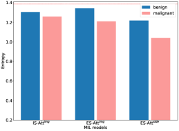
Figure 2: Entropy of attention weight distribution of attention-based models for malignant and benign class for MGM-FV. Red dashed line shows the entropy for uniform weights of all views, e.g., 0.25 for four views.

5.2 MIL vs SIL Performance

To analyse how models trained on case labels compare to models trained on image labels, we compared our best performing MIL model ES-Att${}^{\text{side}}$ to two SIL settings: SIL${}^{\text{IL}}$, where each image has its true label and SIL${}^{\text{CL}}$, where the case label is transferred to all images in that case. CBIS and VinDr contain both image and case labels, whereas MGM contains only the latter, thus SIL${}^{\text{IL}}$ results are not reported on MGM. All our model variants use GMIC as feature extractor and SIL models were trained on the same train-val-test splits as MIL.

Table 5 show that all models trained on case labels either outperform or are on par with models trained on image labels. This suggests that case labels are sufficient for predicting breast cancer and manual labelling of images is not required. The difference is less pronounced for CBIS, which only has 3% of malignant cases where the labels for cases and images do not match, while VinDr has 97% of such cases (cf. Table 3).

Table 5: SIL vs. MIL comparison (F1) on CBIS, VinDr, MGM-VV; SIL (bs=10). Prediction (P), n.a.: image labels are unavailable.

Model	P. Level	CBIS	VinDr	MGM-VV
SIL${}^{\text{IL}}$	Image	$0.66\pm 0.03$	$0.27\pm 0.01$	n.a.
SIL${}^{\text{IL}}$	Case	$\textbf{0.68}\pm 0.03$	$0.30\pm 0.00$	n.a.
SIL${}^{\text{CL}}$	Image	$0.65\pm 0.02$	$0.32\pm 0.05$	$0.44\pm 0.01$
SIL${}^{\text{CL}}$	Case	$0.67\pm 0.02$	$0.26\pm 0.05$	$0.44\pm 0.01$
ES-Att${}^{\text{side}}$	Case	$\textbf{0.68}\pm 0.06$	$\textbf{0.48}\pm 0.03$	$\textbf{0.58}\pm 0.01$

5.3 Analysing the Ability to Identify Relevant Images

To understand to which extent MIL models can identify important, i.e., malignant, images in malignant cases, we analysed the attention scores in MIL models as proxy for the importance given to each image by the MIL model. We converted the attention score to predicted image labels for all truly malignant cases as follows: image $k$ with attention score $a_{k}>0.25$ was assigned malignant, otherwise benign. Then, we calculated the F1 score with respect to the true image-level labels. We performed this evaluation only for malignant cases as all images in a benign case have the same groundtruth. We performed this analysis on VinDr, as this is the largest dataset with known image labels in our paper and has the highest percentage of cases with mixed image labels (Table 3 CL$\neq$IL).

Fig. 3 shows that our domain-specific MIL pooling (ES-Att${}^{\text{side}}$) has the best capability to find the malignant images in malignant cases (F1$=0.82$). All MIL attention models outperform the baseline model, IS-Mean${}^{\text{img}}$ (F1$=0.52$), where all images have equal importance. This shows that case label trained MIL attention models are capable of identifying the malignant images within a malignant case.

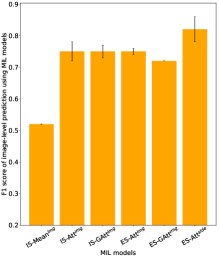
Figure 3: Agreement of images identified as relevant, i.e., malignant (attention score $>0.25$), for truly malignant cases on VinDr.

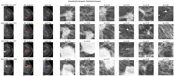
Figure 4: Visualization of a malignant mammogram case from MGM dataset: the case contains 4 images - CC and MLO view from both left and right breast. Each row shows the original mammogram image, the saliency map from the GMIC Global Network (important regions shown in red), extracted ROIs marked on the image (blue) and then the 6 candidate ROIs extracted by our model ES-Att${}^{\text{img}}$. The associated scores of the images and patches are the attention weights assigned by the model. Views from right breast are flipped horizontally for input to the model.

5.4 Variable-image Training

To analyse the impact of variable-image training, we compared ES-Att${}^{\text{img}}$ trained on the dataset with variable views MGM-VV and on its counterpart with only the four standard views MGM-FV, both trained for max. 30 epochs with early stopping (patience epoch 10).

Fig. 5 compares the performance of ES-Att${}^{\text{img}}$ when trained on MGM-FV and tested on MGM-VV (light bars), and trained and tested on MGM-VV (dark bars). We observe that the models trained on variable views, MGM-VV (F1 $=0.59$) slightly outperform the models trained on fixed views, MGM-FV (F1 $=0.58$) overall (group All) and for most groups. Cases with only standard views (std.) have a slightly higher performance than cases with mixed (mix) views, containing both standard and non-standard views. The standard deviation of the F1 score seems to be negatively correlated with the number of cases in each group. We conclude that it is not necessary to train with variable-image cases to obtain a reasonable performance on variable-image cases (including unseen views) during prediction. However, variable-image training slightly improves performance.

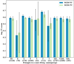
Figure 5: Variable-view performance (F1 score) of ES-Att${}^{\text{img}}$ on MGM. Showing mean and standard deviation (error bar), grouped by the number of images per cases (in brackets).

5.5 Quality of Unsupervised ROI Extraction

We investigate the quality of the unsupervised ROI extractor GMIC [8] both, quantitatively and qualitatively.

For the quantitative assessment, we calculated the intersection over union (IoU) and dice similarity coefficient (DSC) of the extracted ROI candidates with the ROI groundtruth annotations available in the two public datasets CBIS and VinDr. We calculated scores in the MIL setting (ES-Att${}^{\text{side}}$) and its SIL counterpart. In the multi-instance model (ES-Att${}^{\text{side}}$), the IoU is $0.04$ and $0.23$ on CBIS and VinDr, respectively. DSC shows a similar pattern, with $0.05$ and $0.34$ on CBIS and VinDr. In the single-instance model (SIL${}^{\text{IL}}$), both measures show similar ranges to the multi-instance model: IoU $0.04$ and $0.18$, and DSC $0.07$ and $0.28$ on CBIS and VinDr, respectively. The difference in score between the two datasets might be due to the differing image quality.

Additionally, we qualitatively evaluated the ROI candidates for 61 cases from the MGM test set through a semi-structured interview with two radiologists. We divided the cases into four groups: true positive (malignant detected as malignant), false positive (benign detected as malignant), true negative (benign detected as benign) and false negative (malignant detected as benign) cases. Fig. 4 shows an example true positive case from MGM with extracted ROIs. We asked the following questions during the interview. For true positives and false negative cases: “Do you see any relevant ROI among the extracted ROI candidates?” and “Does the relevant ROI have the highest attention score?”. For true negative cases we asked “What kind of patches do you see?” For misclassifications, we asked the radiologists to describe which kind of mistakes were made. Clinicians found the extracted ROIs to be relevant, and confirmed that the patches with abnormalities were extracted for the malignant cases. Anecdotally, radiologists were surprised that the model found the mass abnormality for one of the cases with high breast density, which is usually rather hard to detect for humans. While important ROIs were correctly extracted, they were not always associated with the highest attention score. On the image level, the important images for the decision were more often correctly associated with the highest attention scores. For benign cases, extracted ROIs usually showed normal tissues. For the malignant and benign misclassifications, the radiologists commented that the ROIs correctly identified abnormal tissue, but that the decision on malignant or benign would require additional diagnostic tests.

In summary, the qualitative assessment showed satisfying quality of extracted ROIs for MGM, while the quantitative measures indicate that improving ROI extraction could be a key factor for improving overall model performance.

6 Discussion

Our results show case-level models are on par with image-level models, eliminating the need for manual annotation of images. The comparison to state-of-the-art models on the public benchmark CBIS at image-level shows that our case-level model (ES-Att${}^{\text{img}}$; AUC $=0.81$ custom split, AUC $=0.79$ official split) performs similarly to models trained on image labels [22] (AUC 0.80 official split, without ensemble and test time augmentation). Our end-to-end deep learning based model achieves similar performance to a case-level MIL model trained on hand-crafted features from DDSM [24] and also generalizes across 3 datasets. While Quellec et al. [24] consider abnormalities that are not visible in both views as false alarms, our domain-specific MIL pooling can learn to select the important view for the task. Our overlap score (DSC 0.34 VinDr) between ROIs extracted by the model and the groundtruth ROIs is in the same range as related work [8] (DSC 0.33) and [17] (DSC 0.39) on a private dataset. More investigation is needed for unsupervised ROI extraction such that breast cancer prediction can be made more reliable.

We also observe differences in performance across datasets. Overall, the performance varies from F1 $=0.68$ on CBIS, F1 $=0.60$ on MGM to F1 $=0.48$ on VinDr. Aside from varying data quantity and quality, the difficulty of the classification task can also impact performance. Khan et al. found normal vs. abnormal (benign and malignant) to be easier to classify (AUC $=0.93$) than malignant vs. benign (AUC $=0.84$) on MIAS-CBIS [21]. Similarly, the benign class of CBIS has only benign cases (including benign abnormalities), whereas in MGM it additionally contains normal cases. Classes can also be defined based on BI-RADS score [16] (as followed in VinDr), but this may not reflect the true class of the cases (with a higher chance of some benign cases getting the groundtruth of malignant). This might explain our low performance on VinDr.

Reproducibility and replicability are important aspects of scientific research to achieve scientific progress [47]. We found a gap of 0.03-0.08 in AUC on CBIS while reproducing related work [7, 8]. We call for transparency on hyperparameter settings and the preprocessing details to support reproducibility. We have made our hyperparameters, preprocessing, and training code public¹ to promote reproducibility and to set our work as a benchmark.

The main factors for high performance of case-level breast cancer prediction models are pretraining, unsupervised ROI extraction, choice of MIL pooling, and hyperparameter tuning. First, we found that pretrained models (trained on ImageNet) increase the performance by at least 10%. We have not experimentally verified the claim of achieving higher performance by pretraining models on BI-RADS scores [5, 8], because BI-RADS scores are not readily available in hospital databases. The performance range of our models pretrained on ImageNet (AUC 0.85 MGM) is similar to models pretrained on BI-RADS (AUC 0.82 view-wise model [5] on private dataset), showing that both types of pretraining are beneficial. Second, unsupervised ROI extraction improves performance over global feature extractors for some datasets (we observed a 3% higher AUC for GMIC vs Resnet34 for ES-Att${}^{\text{side}}$ on VinDr). Third, the choice of MIL pooling can impact the F1 score by up to 8% (MGM-FV). Fourth, we found hyperparameter tuning to be important to get good performance. For instance, the AUC score varied from 0.78 to 0.82 for GMIC on official CBIS split among the top-5 settings for model hyperparameters in SIL.

7 Conclusion and Future Work

We propose a foundational framework for case-level breast cancer prediction using mammography that addresses the 3 challenges of realistic clinical settings - groundtruth only available at the case-level, no ROI annotation available and variable number of images per case. Our case-level model achieves similar performance to image-level models, suggesting that time-consuming manual annotation of images is not required. Our domain-specific MIL pooling method is competitive to other MIL pooling methods across 3 datasets and outperforms the other methods in identifying the malignant images in a malignant case. Thus, our MIL model can reliably point out the malignant breast side and image view, which is important for uptake in a clinical workflow. As unsupervised ROI extraction methods cannot yet perfectly detect ROIs, we call to focus on unsupervised ROI extraction, in order to improve breast cancer prediction in realistic settings and hence for the benefit of all patients. In this work, we assume no dependencies among instances. However, an abnormality visible in one view of one breast may also be visible in the other views of that breast. In future work, we aim to incorporate self-attention based methods, which compute the attention weights of a bag by relating instances to each other.

References

- [1] World Health Organization, “Cancer,” https://www.who.int/news-room/fact-sheets/detail/cancer, 2022, accessed: 15/06/2023.
- [2] L. Tabár, B. Vitak, H.-H. T. Chen, M.-F. Yen, S. W. Duffy, and R. A. Smith, “Beyond randomized controlled trials: organized mammographic screening substantially reduces breast carcinoma mortality,” Cancer: Interdisciplinary International Journal of the American Cancer Society, vol. 91, no. 9, pp. 1724–1731, 2001.
- [3] L. Tabár, B. Vitak, T. H.-H. Chen, A. M.-F. Yen, A. Cohen, T. Tot, S. Y.-H. Chiu, S. L.-S. Chen, J. C.-Y. Fann, J. Rosell et al., “Swedish two-county trial: impact of mammographic screening on breast cancer mortality during 3 decades,” Radiology-Radiological Society of North America, vol. 260, no. 3, p. 658, 2011.
- [4] L. Shen, L. R. Margolies, J. H. Rothstein, E. Fluder, R. McBride, and W. Sieh, “Deep learning to improve breast cancer detection on screening mammography,” Scientific reports, vol. 9, no. 1, pp. 1–12, 2019.
- [5] N. Wu, J. Phang, J. Park, Y. Shen, Z. Huang, M. Zorin, S. Jastrzebski, T. Févry, J. Katsnelson, E. Kim, S. Wolfson, U. Parikh, S. Gaddam, L. L. Y. Lin, K. Ho, J. D. Weinstein, B. Reig, Y. Gao, H. Toth, K. Pysarenko, A. Lewin, J. Lee, K. Airola, E. Mema, S. Chung, E. Hwang, N. Samreen, S. G. Kim, L. Heacock, L. Moy, K. Cho, and K. J. Geras, “Deep neural networks improve radiologists’ performance in breast cancer screening,” IEEE Transactions on Medical Imaging, vol. 39, no. 4, p. 1184–1194, Apr 2020.
- [6] T. Kyono, F. J. Gilbert, and M. van der Schaar, “Improving workflow efficiency for mammography using machine learning,” Journal of the American College of Radiology, vol. 17, no. 1, pp. 56–63, 2020.
- [7] X. Shu, L. Zhang, Z. Wang, Q. Lv, and Z. Yi, “Deep neural networks with region-based pooling structures for mammographic image classification,” IEEE transactions on medical imaging, vol. 39, no. 6, pp. 2246–2255, 2020.
- [8] Y. Shen, N. Wu, J. Phang, J. Park, K. Liu, S. Tyagi, L. Heacock, S. G. Kim, L. Moy, K. Cho et al., “An interpretable classifier for high-resolution breast cancer screening images utilizing weakly supervised localization,” Medical image analysis, vol. 68, p. 101908, 2021.
- [9] A. Rampun, B. W. Scotney, P. J. Morrow, and H. Wang, “Breast mass classification in mammograms using ensemble convolutional neural networks,” in 2018 IEEE 20th International Conference on e-Health Networking, Applications and Services (Healthcom). IEEE, 2018, pp. 1–6.
- [10] Z. Wang, L. Zhang, X. Shu, Q. Lv, and Z. Yi, “An end-to-end mammogram diagnosis: A new multi-instance and multiscale method based on single-image feature,” IEEE Transactions on Cognitive and Developmental Systems, vol. 13, no. 3, p. 535–545, Sep 2021.
- [11] D. Lévy and A. Jain, “Breast mass classification from mammograms using deep convolutional neural networks,” arXiv:1612.00542 [cs], Dec 2016, arXiv: 1612.00542.
- [12] W. Zhu, Q. Lou, Y. S. Vang, and X. Xie, “Deep multi-instance networks with sparse label assignment for whole mammogram classification,” in International conference on medical image computing and computer-assisted intervention. Springer, 2017, pp. 603–611.
- [13] C. Zhang, J. Zhao, J. Niu, and D. Li, “New convolutional neural network model for screening and diagnosis of mammograms,” PLoS One, vol. 15, no. 8, p. e0237674, 2020.
- [14] A. Akselrod-Ballin, M. Chorev, Y. Shoshan, A. Spiro, A. Hazan, R. Melamed, E. Barkan, E. Herzel, S. Naor, E. Karavani et al., “Predicting breast cancer by applying deep learning to linked health records and mammograms,” Radiology, vol. 292, no. 2, pp. 331–342, 2019.
- [15] E.-K. Kim, H.-E. Kim, K. Han, B. J. Kang, Y.-M. Sohn, O. H. Woo, and C. W. Lee, “Applying data-driven imaging biomarker in mammography for breast cancer screening: preliminary study,” Scientific reports, vol. 8, no. 1, pp. 1–8, 2018.
- [16] G. Carneiro, J. Nascimento, and A. P. Bradley, “Unregistered multiview mammogram analysis with pre-trained deep learning models,” in International Conference on Medical Image Computing and Computer-Assisted Intervention. Springer, 2015, pp. 652–660.
- [17] K. Liu, Y. Shen, N. Wu, J. Chłędowski, C. Fernandez-Granda, and K. J. Geras, “Weakly-supervised high-resolution segmentation of mammography images for breast cancer diagnosis,” Proceedings of machine learning research, vol. 143, p. 268, 2021.
- [18] K. Rangarajan, A. Gupta, S. Dasgupta, U. Marri, A. K. Gupta, S. Hari, S. Banerjee, and C. Arora, “Ultra-high resolution, multi-scale, context-aware approach for detection of small cancers on mammography,” Scientific Reports, vol. 12, no. 1, p. 11622, 2022.
- [19] L. Tsochatzidis, L. Costaridou, and I. Pratikakis, “Deep learning for breast cancer diagnosis from mammograms—a comparative study,” Journal of Imaging, vol. 5, no. 33, p. 37, Mar 2019.
- [20] D. A. Ragab, O. Attallah, M. Sharkas, J. Ren, and S. Marshall, “A framework for breast cancer classification using multi-dcnns,” Computers in Biology and Medicine, vol. 131, p. 104245, 2021.
- [21] H. N. Khan, A. R. Shahid, B. Raza, A. H. Dar, and H. Alquhayz, “Multi-view feature fusion based four views model for mammogram classification using convolutional neural network,” IEEE Access, vol. 7, pp. 165 724–165 733, 2019.
- [22] T. Wei, A. I. Aviles-Rivero, S. Wang, Y. Huang, F. J. Gilbert, C.-B. Schönlieb, and C. W. Chen, “Beyond fine-tuning: Classifying high resolution mammograms using function-preserving transformations,” Medical Image Analysis, vol. 82, p. 102618, 2022.
- [23] D. G. Petrini, C. Shimizu, R. A. Roela, G. V. Valente, M. A. A. K. Folgueira, and H. Y. Kim, “Breast cancer diagnosis in two-view mammography using end-to-end trained efficientnet-based convolutional network,” Ieee Access, vol. 10, pp. 77 723–77 731, 2022.
- [24] G. Quellec, M. Lamard, M. Cozic, G. Coatrieux, and G. Cazuguel, “Multiple-instance learning for anomaly detection in digital mammography,” Ieee transactions on medical imaging, vol. 35, no. 7, pp. 1604–1614, 2016.
- [25] S. M. McKinney, M. Sieniek, V. Godbole, J. Godwin, N. Antropova, H. Ashrafian, T. Back, M. Chesus, G. S. Corrado, A. Darzi et al., “International evaluation of an ai system for breast cancer screening,” Nature, vol. 577, no. 7788, pp. 89–94, 2020.
- [26] T. G. Dietterich, R. H. Lathrop, and T. Lozano-Pérez, “Solving the multiple instance problem with axis-parallel rectangles,” Artificial intelligence, vol. 89, no. 1-2, pp. 31–71, 1997.
- [27] O. Maron and T. Lozano-Pérez, “A framework for multiple-instance learning,” Advances in neural information processing systems, vol. 10, 1997.
- [28] S. Andrews, I. Tsochantaridis, and T. Hofmann, “Support vector machines for multiple-instance learning,” Advances in neural information processing systems, vol. 15, 2002.
- [29] C. Zhang, J. Platt, and P. Viola, “Multiple instance boosting for object detection,” Advances in neural information processing systems, vol. 18, 2005.
- [30] R. Sawyer-Lee, F. Gimenez, A. Hoogi, and D. Rubin, “Curated breast imaging subset of digital database for screening mammography (cbis-ddsm) (version 1) [data set],” 2016, accessed: 28/04/2022. [Online]. Available: https://doi.org/10.7937/K9/TCIA.2016.7O02S9CY
- [31] M. Heath, K. Bowyer, D. Kopans, P. Kegelmeyer Jr, R. Moore, K. Chang, and S. Munishkumaran, “Current status of the digital database for screening mammography,” in Digital Mammography: Nijmegen, 1998. Springer, 1998, pp. 457–460.
- [32] H. T. Nguyen, H. Q. Nguyen, H. H. Pham, K. Lam, L. T. Le, M. Dao, and V. Vu, “Vindr-mammo: A large-scale benchmark dataset for computer-aided diagnosis in full-field digital mammography,” medRxiv, 2022.
- [33] D. Ribli, A. Horváth, Z. Unger, P. Pollner, and I. Csabai, “Detecting and classifying lesions in mammograms with deep learning,” Scientific reports, vol. 8, no. 1, p. 4165, 2018.
- [34] R. Agarwal, O. Diaz, X. Lladó, M. H. Yap, and R. Martí, “Automatic mass detection in mammograms using deep convolutional neural networks,” Journal of Medical Imaging, vol. 6, no. 3, pp. 031 409–031 409, 2019.
- [35] T. Hu, L. Zhang, L. Xie, and Z. Yi, “A multi-instance networks with multiple views for classification of mammograms,” Neurocomputing, vol. 443, pp. 320–328, 2021.
- [36] E. Raff, “A step toward quantifying independently reproducible machine learning research,” Advances in Neural Information Processing Systems, vol. 32, 2019.
- [37] K. He, X. Zhang, S. Ren, and J. Sun, “Deep residual learning for image recognition,” CoRR, vol. abs/1512.03385, 2015.
- [38] M. Ilse, J. Tomczak, and M. Welling, “Attention-based deep multiple instance learning,” in International conference on machine learning. PMLR, 2018, pp. 2127–2136.
- [39] Y. Chen, J. Bi, and J. Z. Wang, “Miles: Multiple-instance learning via embedded instance selection,” IEEE Transactions on Pattern Analysis and Machine Intelligence, vol. 28, no. 12, pp. 1931–1947, 2006.
- [40] X.-S. Wei, J. Wu, and Z.-H. Zhou, “Scalable algorithms for multi-instance learning,” IEEE transactions on neural networks and learning systems, vol. 28, no. 4, pp. 975–987, 2016.
- [41] J. Foulds and E. Frank, “A review of multi-instance learning assumptions,” The Knowledge Engineering Review, vol. 25, no. 1, p. 1–25, Mar 2010.
- [42] J. Amores, “Multiple instance classification: Review, taxonomy and comparative study,” Artificial intelligence, vol. 201, pp. 81–105, 2013.
- [43] X. Wang, Y. Yan, P. Tang, X. Bai, and W. Liu, “Revisiting multiple instance neural networks,” Pattern Recognition, vol. 74, pp. 15–24, 2018.
- [44] D. P. Kingma and J. Ba, “Adam: A method for stochastic optimization,” 2017.
- [45] E. A. Sickles, C. J. D’Orsi, L. W. Bassett, C. M. Appleton, W. A. Berg, E. S. Burnside et al., “Acr bi-rads® mammography,” ACR BI-RADS® atlas, breast imaging reporting and data system, vol. 5, p. 2013, 2013.
- [46] O. S. Pianykh, Digital Imaging and Communications in Medicine (DICOM): A Practical Introduction and Survival Guide, 1st ed. Springer Publishing Company, Incorporated, 2010.
- [47] D. Ulmer, E. Bassignana, M. Müller-Eberstein, D. Varab, M. Zhang, R. van der Goot, C. Hardmeier, and B. Plank, “Experimental standards for deep learning in natural language processing research,” in Findings of the Association for Computational Linguistics: EMNLP 2022. Association for Computational Linguistics, Dec 2022, p. 2673–2692.