Inverse Renormalization Group of Disordered Systems

Abstract

We propose inverse renormalization group transformations to construct approximate configurations for lattice volumes that have not yet been accessed by supercomputers or large-scale simulations in the study of spin glasses. Specifically, starting from lattices of volume $V=8^{3}$ in the case of the three-dimensional Edwards-Anderson model we employ machine learning algorithms to construct rescaled lattices up to $V^{\prime}=128^{3}$, which we utilize to extract two critical exponents. We conclude by discussing how to incorporate numerical exactness within inverse renormalization group approaches of disordered systems, thus opening up the opportunity to explore a sustainable and energy-efficient generation of exact configurations for increasing lattice volumes without the use of dedicated supercomputers.

Introduction.—

The spin glass [1, 2, 3] has posed some of the greatest challenges to the community of statistical mechanics and to computational physicists. Direct Monte Carlo simulations of spin glasses with the Metropolis algorithm fail to thermalize in sufficient computational time as one approaches the spin glass phase. One must then shift to methods which rely on the exchange of configurations between a large number of simulations: these limit the computational resources available to study spin glasses. To exacerbate the above problems, calculations of expectation values for spin glasses require an additional averaging over a large number of realizations of disorder, further limiting the computational power which can be employed to gain insights into the physical behavior of these systems.

Nevertheless, the spin glass is an intrinsically interesting topic. To study spin glasses, and more generally disordered systems, one must investigate the behavior of a system which manifests some form of inconsistency or imperfection in its construction. Spin glasses have a direct connection with the experimental aspect of science. Disorder, more generally, emerges in all subfields of physics. It is of interest that the above concepts extend beyond physical problems and are relevant for topics such as combinatorial optimization, neural networks, or multi-agent systems [1]. Given the broad impact of spin glasses in the mathematical and physical sciences, it is of vital importance that we extend the framework of statistical physics in order to accelerate the computational studies of these systems [4].

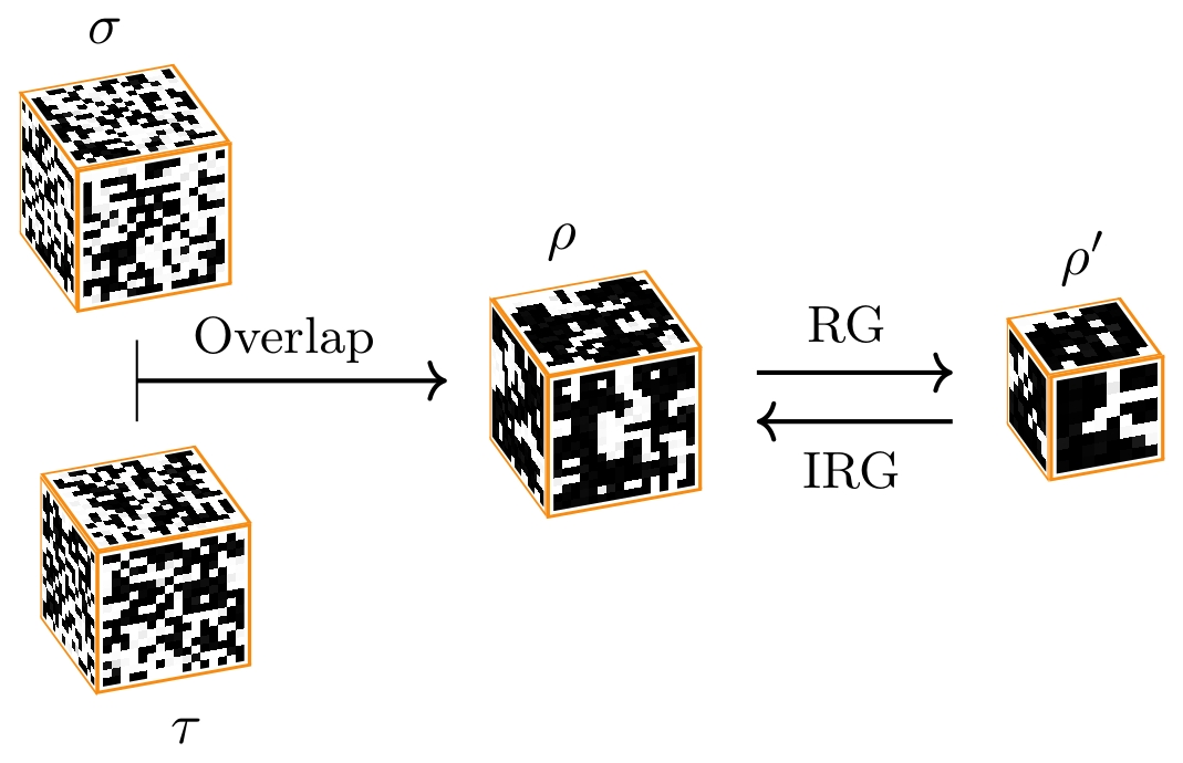
Figure 1: The inversion of a standard renormalization group transformation with the use of machine learning. Two replicas $\sigma$, $\tau$ are mapped to an overlap configuration $\rho$ which is renormalized (RG) via the majority rule to obtain $\rho^{\prime}$. The standard renormalization group is then inverted (IRG) with the use of convolutions to reproduce $\rho$ from $\rho^{\prime}$.

In this manuscript we introduce inverse renormalization group transformations to spin glasses. Starting from lattices of volume $V=8^{3}$ in the case of the three-dimensional Edwards-Anderson model we apply a set of inverse transformations to construct lattices of volume $V^{\prime}=128^{3}$. The method is implemented on an effective Hamiltonian which comprises overlap degrees of freedom [5, 6, 7, 8], and approximates the inversion of a standard renormalization group transformation, suitable for the study of disordered systems [9, 10, 11], with machine learning algorithms. We additionally explore if the method is capable of producing approximate configurations for lattice volumes that have not yet been accessed by supercomputers and large-scale simulations in the study of spin glasses [12, 13].

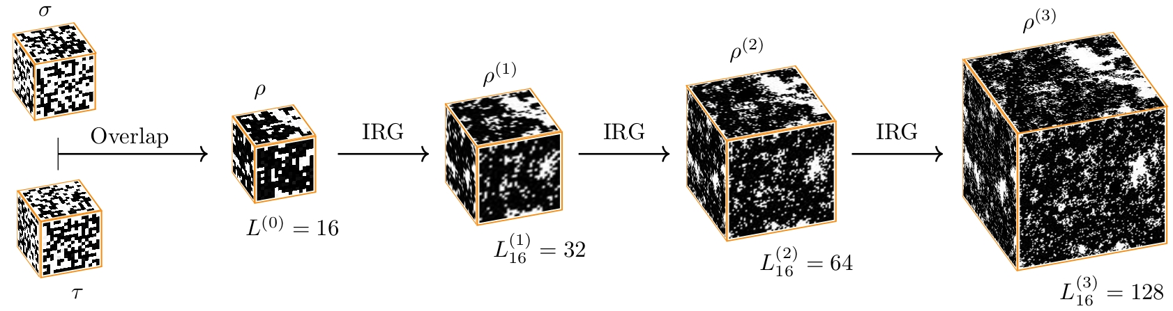
Figure 2: Application of the inverse renormalization group. Two replicas $\sigma$, $\tau$ are mapped to an overlap configuration $\rho$. Inverse renormalization group transformations are applied iteratively to construct equilibrated configurations $\rho^{(1)}$, $\rho^{(2)}$ and $\rho^{(3)}$ up to lattice volumes $V=128^{3}$ without requiring additional Monte Carlo simulations on the larger lattices.

Inverse renormalization group methods have been implemented before in statistical physics or quantum field theory [14, 15, 16, 17, 18, 19] but, to our knowledge, this manuscript documents the first use of the inverse renormalization group to study a disordered system. Previous implementations, which in principle enable the iterative generation of configurations for increasing lattice size, are limited to applications on exactly-solvable models or systems for which the critical fixed point is known to high numerical accuracy: examples are the Ising model [14, 16, 18] and the $\phi^{4}$ theory [15]. In comparison to spin glasses, the aforementioned systems can be easily simulated, in high dimensions and to large lattice volumes. Consequently, we explore if, by generating approximate configurations for lattice volumes that are not accessible by supercomputers and large-scale simulations, this manuscript documents the first implemenentation of the inverse renormalization group to obtain a result that is, at the time of writing, inaccessible by other computational means.

To establish the method, we additionally extend the two-lattice matching renormalization group approach [20, 21, 22, 10, 23] to the inverse case and we extract two critical exponents. We conclude by outlining how to incorporate numerical exactness within inverse renormalization group methods of disordered systems, thus opening up the opportunity to explore a sustainable and energy-efficient generation of exact configurations for increasing lattice volumes without the use of dedicated supercomputers.

Transitioning to overlap configurations.—

We consider the three-dimensional Edwards-Anderson model with helical boundary conditions and two replicas $\sigma$, $\tau$ which comprise spins $s$, $t$. The system is described by the two-replica Hamiltonian:

$$E_{\sigma,\tau}=E_{\sigma}+E_{\tau}=-\sum_{\langle ij\rangle}J_{ij}(s_{i}s_{j}+t_{i}t_{j}),$$ (1)

where $s,t=\pm 1$, $\langle ij\rangle$ corresponds to nearest-neighbors $i$ and $j$, $J_{ij}$ is a random coupling sampled with equal probability as $J_{ij}=\pm 1$, and the set $\{J_{ij}\}$ defines a given realization of disorder for the system.

The Boltzmann probability distribution $p_{\sigma_{i},\tau_{j}}$ of sampling two configurations $\sigma_{i}$, $\tau_{j}$ at inverse temperature $\beta$ is:

$$p_{\sigma_{i},\tau_{j}}=\frac{\exp[-\beta(E_{\sigma_{i}}+E_{\tau_{j}})]}{\sum_{\sigma}\sum_{\tau}\exp[-\beta(E_{\sigma}+E_{\tau})]},$$ (2)

where $Z^{2}=\sum_{\sigma}\sum_{\tau}\exp[-\beta(E_{\sigma}+E_{\tau})]$ is the partition function and the sums are over all possible configurations $\sigma$, $\tau$.

The spin glass phase transition of the system is characterized by an overlap order parameter [24, 25, 26, 27] which is defined over two replicas $\sigma$, $\tau$:

$$q_{\sigma\tau}=\frac{1}{V}\sum_{i}s_{i}t_{i},$$ (3)

where $V=L^{3}$ is the volume of the system and $L$ the lattice size in each dimension. Another quantity of interest is the overlap susceptibility $\chi$:

$$\chi=\beta V(\langle q^{2}\rangle-\langle q\rangle^{2})=\beta V\langle q^{2}\rangle,$$ (4)

where $\langle q\rangle=0$.

We are now interested in mapping the two-replica Edwards-Anderson model with configurations $\sigma$, $\tau$ to an effective system, with configuration $\rho$, which comprises overlap degrees of freedom $\varrho_{i}=s_{i}t_{i}$. This mapping, introduced by Haake-Lewenstein-Wilkens [5], defines an effective Hamiltonian $E^{\textrm{eff}}_{\rho}$, partition function $Z^{\textrm{eff}}_{\rho}$, and Boltzmann probability distribution $P_{\rho_{i}}$ which is averaged over disorder:

$$P_{\rho_{i}}=2^{V}\Bigg{[}\frac{\exp\big{[}\beta\sum_{\langle ij\rangle}J_{ij}(1+\varrho_{i}\varrho_{j})\big{]}}{Z^{2}[\{J_{ij}\}]}\Bigg{]}_{J_{ij}}.$$ (5)

We observe that the emergence of the overlap order parameter $q$ in the two-replica Hamiltonian is equivalent to the emergence of a magnetization $m$, summed over the overlap degrees of freedom, in the effective system:

$$m_{\rho}=\frac{1}{V}\sum_{i}\varrho_{i}=\frac{1}{V}\sum_{i}s_{i}t_{i}=q_{\sigma\tau}.$$ (6)

Equivalently, the spin glass phase transition of the two-replica Edwards-Anderson model is mapped to a phase transition which resembles ferromagnetic ordering in the effective system. Our aim is to approximate the inversion of standard renormalization group implementations [9, 10, 11] on the overlap degrees of freedom.

Inverse renormalization group.—

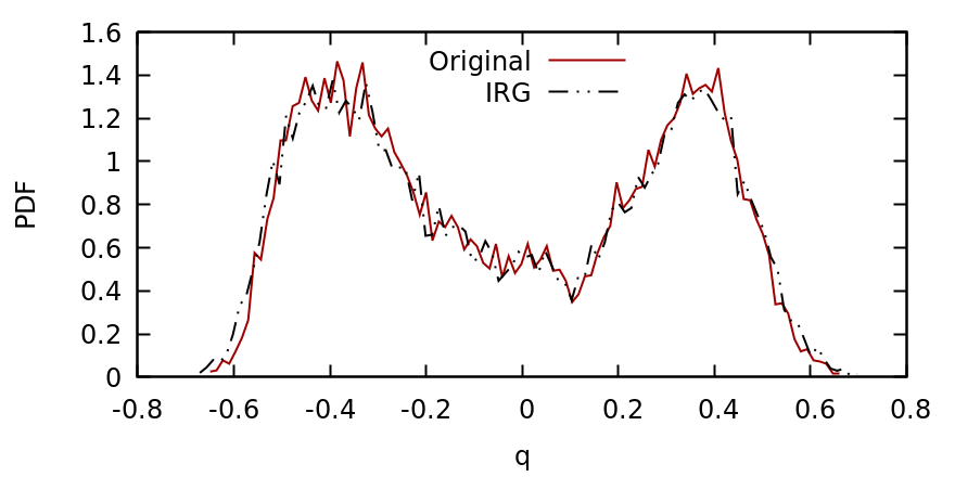
Figure 3: The probability density function of the overlap order parameter $q$ for $\beta=0.9$ and a given realization of disorder $\{J_{ij}\}$. The results are obtained based on original configurations of lattice size $L=16$ and configurations obtained by applying and then inverting a standard renormalization group transformation.

We define a standard renormalization group transformation on the effective probability distribution of the overlap configurations as:

$$P^{\prime}_{\rho^{\prime}}=\sum_{\rho}T(\rho^{\prime},\rho)P_{\rho},$$ (7)

where $T(\rho^{\prime},\rho)$ is a kernel which, in this manuscript, corresponds to the majority rule. A standard renormalization group transformation reduces, in terms of lattice units, the lattice size $L$ and the correlation length $\xi$ of the original system by a rescaling factor of $b$, as $L^{\prime}={L}/{b},$ $\xi^{\prime}={\xi}/{b}$.

We approximate the inversion of this standard transformation via the use of machine learning algorithms. Explicitly, we are interested in learning a kernel $\mathcal{T}(\rho,\rho^{\prime},\{{w}\})$, where $\{w\}$ is a set of variational parameters, to approximately reproduce the original effective probability distribution based on the renormalized one:

$$P_{\rho}=\sum_{\rho^{\prime}}\mathcal{T}(\rho,\rho^{\prime},\{w\})P^{\prime}_{\rho^{\prime}},$$ (8)

The use of machine learning simply concerns the learning of the most accurate values of $\{w\}$ which are able to successfully approximate the inversion of the standard transformation. Equivalently, we aim to learn the most accurate values of $\{w\}$ such that $\mathcal{T}\approx T^{-1}$. Starting from a renormalized configuration $\rho^{\prime}$ with lattice size $L^{\prime}$ and correlation length $\xi^{\prime}$ we use the inverse renormalization group to reconstruct the original configuration $\rho$ with lattice size $L=bL^{\prime}$ and correlation length $\xi=b\xi^{\prime}$. The training process is summarized in Fig. 1.

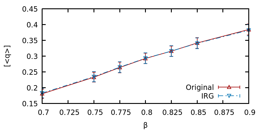
Figure 4: Absolute value of the overlap order parameter $q$, calculated under a thermal and disorder average, versus the inverse temperature $\beta$. The results are obtained based on original configurations of lattice size $L=16$ and model configurations obtained by applying and then inverting a standard renormalization group transformation.

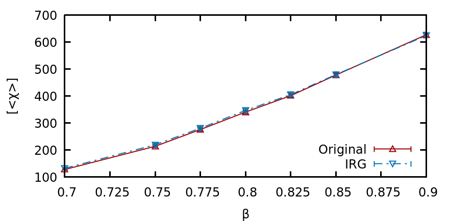
Figure 5: Overlap susceptibility $\chi$, calculated under a thermal and disorder average, versus the inverse temperature $\beta$. The results are obtained based on original configurations of lattice size $L=16$ and model configurations obtained by applying and then inverting a standard renormalization group transformation.

There exist two advantages in this method. The first is that one can verify, a priori, that a standard renormalization group transformation can be implemented successfully to study the phase transition of the system before one decides to proceed with the inversion. As a result, one is able to establish that, via the machine learning approach, one obtains an inverse transformation which will be equally successful in studying the phase transition as the standard transformation. It is already established that the majority rule is a suitable standard transformation for the effective spin glass system [10, 11]. The second advantage of the method is that if one employs a machine learning algorithm, such as a set of convolutions, which can be applied irrespective of a given lattice size then one is able to iteratively increase, in principle for an arbitrary number of times, the lattice size and the correlation length of the system by a factor of $b$. Formally:

$$P^{(n+1)}_{\rho^{(n+1)}}=\sum_{\rho^{(n)}}\mathcal{T}(\rho^{(n+1)},\rho^{(n)},\{w\})P^{(n)}_{\rho^{(n)}},$$ (9)

where $n\geq 0$ is the number of iterative renormalization group transformations and $P^{0}\equiv P$ is the probability distribution of an original system with overlap configurations $\rho^{0}\equiv\rho$. In this manuscript, we consider a rescaling factor of $b=2$. This process, of iteratively increasing the lattice size by a factor of two, is illustrated in Fig. 2.

To train the machine learning algorithm we sample a set of configurations for lattice size $L=16$ with the parallel tempering technique [28] and apply the majority rule on the overlap degrees of freedom to obtain configurations of $L^{\prime}=8$. We then minimize a binary cross-entropy function by presenting the overlap configurations from $L^{\prime}=8$ as input to the machine learning algorithm and the overlap configurations of $L=16$ as the desired output. The data used to train the machine learning algorithm are then discarded. The output of the machine learning algorithm corresponds to the probability that each rescaled degree of freedom $\rho_{i}^{\prime}$ is assigned the value of $1$. We sample probabilistically the rescaled degrees of freedom, thus verifying that all possible configurations for all possible realizations of disorder have a non-zero probability of appearing. Details about the machine learning implementation [29, 30] and the data analysis are discussed in the Supplemental Material .

After the training is completed, the machine learning algorithm has learned how to approximate the inversion of a standard renormalization group transformation. To verify that the inverse renormalization group is successful we start by sampling a set of configurations for lattice size $L=16$ and apply the standard renormalization group transformation $T$ on the overlap degrees of freedom to produce overlap configurations of lattice size $L^{\prime}=8$. The inverse renormalization group $\mathcal{T}$ is then applied on the overlap configurations of $L^{\prime}=8$ to obtain model configurations of lattice size $L=16$. We calculate $q$ and $\chi$ on the original and the model configurations of $L=16$. We anticipate that, if the inverse renormalization group implementation is successful, the observables should agree within errors.

The results, obtained by applying and then inverting the standard renormalization group transformation, are depicted in Figs. 3, 4, and 5. We observe in Fig. 3 that, for a given realization of disorder $\{J_{ij}\}$, the inverse renormalization group reproduces accurately the probability density function of the overlap order parameter $q$. We then observe in Figs. 4 and 5 that the overlap order parameter $q$ and the overlap susceptibility $\chi$, which are calculated under a thermal $\langle\rangle$ and disorder $[]$ average for original and model configurations, are in agreement within statistical errors. These observations verify that the machine learning algorithm has learned how to approximate the inversion of a standard renormalization group transformation which implements the majority rule.

The critical exponents.—

Via the inverse renormalization group we are able to directly construct approximate configurations of increasing lattice size and correlation length. This implies that it is not necessary to implement Monte Carlo simulations on larger systems to obtain configurations. We now employ the inverse renormalization group transformations to extract multiple critical exponents for the spin glass phase transition of the three-dimensional Edwards-Anderson model.

To establish the validity of inverse renormalization group methods in disordered systems we extend the two lattice matching renormalization group method [20, 21, 22, 10, 23] to the inverse case. Specifically we conduct comparisons for observables of two renormalized systems with identical lattice sizes $L^{(n+1)}$ and $L^{(n)}$ where $n$ is the number of inverse renormalization group transformations. To clarify, we consider systems with lattice sizes $L=8$ and $L=16$ and apply $n$ iterative inverse transformations. We then compare correlation functions for systems with $L^{(2)}_{8}=L^{(1)}_{16}=32$, $L^{(3)}_{8}=L^{(2)}_{16}=64$, and $L^{(4)}_{8}=L^{(3)}_{16}=128$. A similar technique [15], applied to inverse renormalization group methods for quantum field theories, concerns the comparison of observables for a renormalized and an original system: the two methods are not equivalent.

Figure 6: Absolute value of the overlap order parameter $q$, calculated under a thermal and disorder average, versus the inverse temperature $\beta$. The notation $L^{(n)}_{L_{0}}$ denotes a rescaled lattice which is obtained from $L_{0}$ after $n$ iterative inverse renormalization group transformations.

The results, obtained by extending the two lattice matching renormalization group to the inverse case, are depicted in Fig. 6. The figure depicts the overlap order parameter $q$ for systems with lattice sizes $L^{(4)}_{8}=L^{(3)}_{16}=128$. We observe that the intersection of observables indicates the presence of a critical fixed point $\beta_{c}$. In addition, we observe inverse renormalization group flows in parameter space. Specifically, when $\beta<\beta_{c}$, $|q^{(n+1)}|>|q^{(n)}|$. Conversely, when $\beta>\beta_{c}$, $|q^{(n+1)}|<|q^{(n)}|$. This is the anticipated behavior: the renormalized system of $n+1$ inverse transformations has larger correlation length, both below and above the fixed point, when compared with the system of $n$ inverse transformations. Consequently, the renormalized system of $n+1$ iterative inverse transformations resides closer to the fixed point [15]. We remark that the above statements, pertinent to the renormalization group flows, are established in a one-dimensional parameter space. This is achieved under the approximation that the renormalized Hamiltonian is an accurate representation of the original system at a different inverse temperature $\beta$.

We now proceed to calculate numerically the critical exponents $\beta_{q}/\nu$, $\gamma/\nu$ of the overlap order parameter $q$ and the overlap susceptibility $\chi$ via [15]:

$$\frac{\beta_{q}}{\nu}=-\frac{\log\frac{dq_{n+1}}{dq_{n}}}{\ln b},\ \frac{\gamma}{\nu}=\frac{\log\frac{d\chi_{n+1}}{d\chi_{n}}}{\ln b}.$$ (10)

To conduct the calculations we use the absolute value of the overlap order parameter.

The results are summarized in Table  1. We remark that, via the use of scaling relations, the calculations of the two exponents, conducted up to lattice volume $V=128^{3}$, are in agreement with prior standard renormalization group implementations [10, 11]. In addition, the values of the critical exponents agree with large-scale simulations and calculations obtained via supercomputers [12, 13], which simulate lattices up to $V=24^{3}$ and $V=40^{3}$. By employing the inverse renormalization group to construct lattices up to volumes of $V=128^{3}$ which are, at the time of writing, inaccessible by supercomputers and large-scale simulations, we are able to significantly reduce finite-size effects and reduce pertinent systematic errors in the calculations of critical exponents. We remark that the value of the critical fixed point is dependent on the choice of the transformation and is therefore unphysical [32]: it is only the values of the critical exponents that should be attributed any physical significance.

$L=8$	$16/8$	$32/16$	$64/32$	$128/64$
$\beta_{q}/\nu$	$0.28(6)$	$0.29(5)$	$0.30(5)$	$0.30(5)$
$\gamma/\nu$	$2.28(3)$	$2.29(3)$	$2.34(3)$	$2.39(4)$
$L=16$	-	$32/16$	$64/32$	$128/64$
$\beta_{q}/\nu$	-	$0.26(3)$	$0.29(2)$	$0.30(2)$
$\gamma/\nu$	-	$2.35(2)$	$2.33(3)$	$2.38(3)$

Table 1: Calculations of the critical exponents $\beta_{q}/\nu$ and $\gamma/\nu$. The results are obtained from two independent implementations of the inverse renormalization group, one starting from an original lattice of $L=8$ and another from $L=16$.

Conclusions.—

We have introduced inverse renormalization group methods to spin glasses and to disordered systems. Specifically, starting from lattices of volume $V=8^{3}$ in the case of the three-dimensional Edwards-Anderson model we employed a set of inverse transformations to construct approximate configurations for lattices of volume $V=128^{3}$. In addition, we extended the two-lattice matching renormalization group to the inverse case and extracted two critical exponents for the phase transition of the three-dimensional Edwards-Anderson model.

Inverse renormalization group methods overcome the critical slowing down effect [14, 15, 19]. By explicitly constructing approximate configurations of increasing lattice size, and without requiring additional Monte Carlo simulations, the inverse renormalization group evades the need for replica exchange methods in the larger system. Since the method enables the generation of approximate configurations which have not yet been accessed by supercomputers or large-scale simulations it can be implemented to predict, under a significant reduction of finite-size effects, the physical behavior of a system before it becomes known via first-principles calculations.

There exist three impediments to be overcome in order to recast the inverse renormalization group of disordered systems as a numerically exact method and produce exact configurations of the inversely renormalized system. These are the determination of the random couplings which describe the effective system of Eq. 5, the conception of an inverse transformation for the overlap degrees of freedom, and the proposal of an inverse renormalization for the effective realization of disorder. The determination of the random couplings of the effective system is already solved by Wang and Swendsen [33]. The current manuscript proposes a solution to the conception of an inverse transformation for the overlap degrees of freedom. Consequently, the remaining requirement in order to establish numerical exactness is to devise an inverse renormalization for the effective random couplings. Once this is achieved one can introduce the configurations as proposed moves within a Monte Carlo setting. Another approach concerns the introduction of reweighting as a correction step between probability distributions [34, 35] in order to obtain corrected expectation values of observables.

By incorporating numerical exactness, the inverse renormalization group has the potential to achieve a sustainable and energy-efficient generation of exact configurations for lattice sizes that are inaccessible by supercomputers or large-scale simulations, thus providing substantial computational benefits in comparison to conventional Monte Carlo simulations within one of the most numerically challenging research fields of physics, namely the theory of disordered systems.

The author thanks Giulio Biroli for interesting discussions and acknowledges support from the CFM-ENS Data Science Chair and PRAIRIE (the PaRis Artificial Intelligence Research InstitutE).

Supplemental Material

In the application of a standard renormalization group transformation we associate to a block of original degrees of freedom $\{\rho_{1},\ldots,\rho_{b^{3}}\}$ a rescaled degree of freedom $\rho^{\prime}$ in the reduced lattice size $L^{\prime}=L/b$. In contrast, in the inverse renormalization group, we associate to each original degree of freedom $\rho$ a rescaled block of spins $\{\rho_{1}^{\prime},\ldots,\rho_{b^{3}}^{\prime}\}$ in the larger lattice size $L^{\prime}=bL$. Initially, we consider that each of the rescaled degrees of freedom $\{\rho_{1}^{\prime},\ldots,\rho_{b^{3}}^{\prime}\}$, which will be subsequently processed by a set of convolutions, has an identical value as the original degree of freedom $\rho$.

The machine learning algorithm implements three sets of three-dimensional convolutions with $8$ filters, a filter size of $3\times 3\times 3$, a stride of $1$, and a rectified linear unit function $g(x)=\max(0,x)$. These are then followed by another three-dimensional convolution with $1$ filter, a filter size of $2\times 2\times 2$, a stride of $1$, and a sigmoid function $sig(x)=1/(1+\exp[-x])$. To train the machine learning algorithm we first map the values of the degrees of freedom $\{-1,1\}$ to $\{0,1\}$ before presenting them as input. The loss function to be minimized is a binary cross-entropy function. We implement the adaptive moment estimation optimization algorithm with a learning rate of $10^{-5}$, a batch size of $10$ and early stopping. We interpret the output of the machine learning algorithm , which is bound between $[0,1]$, as the probability $p(\rho_{i}^{\prime}=1)$ that the value $\rho^{\prime}_{i}$ in each lattice site $i$ has a value of $1$. We then sample a random number $X$ from a uniform probability distribution $X\sim U[0,1)$. If $p(\rho_{i}^{\prime}=1)\geq X$ we select $\rho_{i}^{\prime}=1$ or if $p(\rho_{i}^{\prime}=1)<X$ we select the rescaled degree of freedom as $\rho_{i}^{\prime}=-1$.

To obtain configurations of the three-dimensional Edwards-Anderson model we use the parallel tempering technique on a set of $19$ inverse temperatures $\beta\in[0.55,1.15]$. For the data depicted in the manuscript we consider $15$ and $30$ realizations of disorder $\{J_{ij}\}$ for lattice sizes $L=16$ and $L=8$, respectively. We create a training dataset by combining configurations from each $\beta\in[0.55,1.15]$ and for three distinct realizations of disorder. The configurations selected are minimally correlated: the machine learning algorithm therefore avoids learning the correlations of the data as a meaningful feature. For the training process, we sample configurations for lattice size $L=16$ and apply the majority rule on the overlap degrees of freedom to obtain configurations of $L^{\prime}=8$. We then present the configurations from $L^{\prime}=8$ as input and the configurations of $L=16$ as the desired output. After the training is completed, we discard all the data and use novel configurations which are obtained from different realizations of disorder than the ones employed to construct the training dataset.

References

- Mézard et al. [1987] M. Mézard, G. Parisi, and M. A. Virasoro, Spin Glass Theory and Beyond: An Introduction to the Replica Method and Its Applications (World Scientific, Singapore, 1987).
- Binder and Young [1986] K. Binder and A. P. Young, Spin glasses: Experimental facts, theoretical concepts, and open questions, Rev. Mod. Phys. 58, 801 (1986).
- Young [1998] A. Young, Spin Glasses and Random Fields, Directions in condensed matter physics (World Scientific, 1998).
- Bhatt and Young [1985] R. N. Bhatt and A. P. Young, Search for a transition in the three-dimensional j ising spin-glass, Phys. Rev. Lett. 54, 924 (1985).
- Haake et al. [1985] F. Haake, M. Lewenstein, and M. Wilkens, Relation of random and competing nonrandom couplings for spin-glasses, Phys. Rev. Lett. 55, 2606 (1985).
- Biroli et al. [2014] G. Biroli, C. Cammarota, G. Tarjus, and M. Tarzia, Random-field-like criticality in glass-forming liquids, Phys. Rev. Lett. 112, 175701 (2014).
- Biroli et al. [2018a] G. Biroli, C. Cammarota, G. Tarjus, and M. Tarzia, Random-field ising-like effective theory of the glass transition. i. mean-field models, Phys. Rev. B 98, 174205 (2018a).
- Biroli et al. [2018b] G. Biroli, C. Cammarota, G. Tarjus, and M. Tarzia, Random field ising-like effective theory of the glass transition. ii. finite-dimensional models, Phys. Rev. B 98, 174206 (2018b).
- Southern and Young [1977] B. W. Southern and A. P. Young, Real space rescaling study of spin glass behaviour in three dimensions, Journal of Physics C: Solid State Physics 10, 2179 (1977).
- Wang and Swendsen [1988a] J.-S. Wang and R. H. Swendsen, Monte carlo renormalization-group study of ising spin glasses, Phys. Rev. B 37, 7745 (1988a).
- Bachtis [2023] D. Bachtis, Overlap renormalization group transformations for disordered systems 10.48550/arxiv.2302.08459 (2023).
- Katzgraber et al. [2006] H. G. Katzgraber, M. Körner, and A. P. Young, Universality in three-dimensional ising spin glasses: A monte carlo study, Phys. Rev. B 73, 224432 (2006).
- Baity-Jesi et al. [2013] M. Baity-Jesi, R. A. Baños, A. Cruz, L. A. Fernandez, J. M. Gil-Narvion, A. Gordillo-Guerrero, D. Iñiguez, A. Maiorano, F. Mantovani, E. Marinari, V. Martin-Mayor, J. Monforte-Garcia, A. M. n. Sudupe, D. Navarro, G. Parisi, S. Perez-Gaviro, M. Pivanti, F. Ricci-Tersenghi, J. J. Ruiz-Lorenzo, S. F. Schifano, B. Seoane, A. Tarancon, R. Tripiccione, and D. Yllanes (Janus Collaboration), Critical parameters of the three-dimensional ising spin glass, Phys. Rev. B 88, 224416 (2013).
- Ron et al. [2002] D. Ron, R. H. Swendsen, and A. Brandt, Inverse monte carlo renormalization group transformations for critical phenomena, Phys. Rev. Lett. 89, 275701 (2002).
- Bachtis et al. [2022] D. Bachtis, G. Aarts, F. Di Renzo, and B. Lucini, Inverse renormalization group in quantum field theory, Phys. Rev. Lett. 128, 081603 (2022).
- Efthymiou et al. [2019] S. Efthymiou, M. J. S. Beach, and R. G. Melko, Super-resolving the ising model with convolutional neural networks, Phys. Rev. B 99, 075113 (2019).
- Li and Wang [2018] S.-H. Li and L. Wang, Neural network renormalization group, Phys. Rev. Lett. 121, 260601 (2018).
- Shiina et al. [2021] K. Shiina, H. Mori, Y. Tomita, H. K. Lee, and Y. Okabe, Inverse renormalization group based on image super-resolution using deep convolutional networks, Scientific Reports 11, 9617 (2021).
- Marchand et al. [2022] T. Marchand, M. Ozawa, G. Biroli, and S. Mallat, Wavelet conditional renormalization group (2022).
- Swendsen [1982] R. H. Swendsen, Phase transitions : Cargese 1980 / edited by Maurice Levy and Jean-Claude Le Guillou and Jean Zinn-Justin (Plenum Press : NATO Scientific Affairs Division New York, 1982).
- Wilson [1980] K. G. Wilson, in Recent Developments in Gauge Theories, edited by G. Hooft, C. Itzykson, A. Jaffe, H. Lehmann, P. K. Mitter, I. M. Singer, and R. Stora (Springer New York, New York, 1980).
- Pawley et al. [1984] G. S. Pawley, R. H. Swendsen, D. J. Wallace, and K. G. Wilson, Monte Carlo renormalization-group calculations of critical behavior in the simple-cubic Ising model, Phys. Rev. B 29, 4030 (1984).
- Bachtis [2022] D. Bachtis, Reducing finite-size effects in quantum field theories with the renormalization group 10.48550/arxiv.2205.08156 (2022).
- Parisi [1979] G. Parisi, Infinite number of order parameters for spin-glasses, Phys. Rev. Lett. 43, 1754 (1979).
- Parisi [1983] G. Parisi, Order parameter for spin-glasses, Phys. Rev. Lett. 50, 1946 (1983).
- Mézard et al. [1984] M. Mézard, G. Parisi, N. Sourlas, G. Toulouse, and M. Virasoro, Nature of the spin-glass phase, Phys. Rev. Lett. 52, 1156 (1984).
- Edwards and Anderson [1975] S. F. Edwards and P. W. Anderson, Theory of spin glasses, Journal of Physics F: Metal Physics 5, 965 (1975).
- Hukushima and Nemoto [1996] K. Hukushima and K. Nemoto, Exchange monte carlo method and application to spin glass simulations, Journal of the Physical Society of Japan 65, 1604 (1996), https://doi.org/10.1143/JPSJ.65.1604 .
- Goodfellow et al. [2016] I. J. Goodfellow, Y. Bengio, and A. Courville, Deep Learning (MIT Press, Cambridge, MA, USA, 2016) http://www.deeplearningbook.org.
- Dumoulin and Visin [2018] V. Dumoulin and F. Visin, A guide to convolution arithmetic for deep learning (2018), arXiv:1603.07285 [stat.ML] .
- Note [1] See Supplemental Material at [URL will be inserted by publisher] for details about the machine learning architecture and the data analysis.
- Swendsen [1979] R. H. Swendsen, Monte carlo renormalization group, Phys. Rev. Lett. 42, 859 (1979).
- Wang and Swendsen [1988b] J.-S. Wang and R. H. Swendsen, Monte carlo and high-temperature-expansion calculations of a spin-glass effective hamiltonian, Phys. Rev. B 38, 9086 (1988b).
- Ferrenberg and Swendsen [1988] A. M. Ferrenberg and R. H. Swendsen, New monte carlo technique for studying phase transitions, Phys. Rev. Lett. 61, 2635 (1988).
- Ytreberg and Zuckerman [2008] F. M. Ytreberg and D. M. Zuckerman, A black-box re-weighting analysis can correct flawed simulation data, Proceedings of the National Academy of Sciences 105, 7982 (2008).