Translation-Invariant Gibbs measures for the Hard Core model with a countable set of spin values

Abstract.

In this paper, we study the Hard Core (HC) model with a countable set $\mathbb{Z}$ of spin values on a Cayley tree of order $k=2$. This model is defined by a countable set of parameters (that is, the activity function $\lambda_{i}>0$, $i\in\mathbb{Z}$). A functional equation is obtained that provides the consistency condition for finite-dimensional Gibbs distributions. Analyzing this equation, the following results are obtained:

• Let $k\geq 2$ and $\Lambda=\sum_{i}\lambda_{i}$. For $\Lambda=+\infty$ there is no translation-invariant Gibbs measure (TIGM);

• Let $k=2$ and $\Lambda<+\infty$. For the model under constraint such that at $G$-admissible graph the loops are imposed at two vertices of the graph, the uniqueness of TIGM is proved;

• Let $k=2$ and $\Lambda<+\infty$. For the model under constraint such that at $G$-admissible graph the loops are imposed at three vertices of the graph, the uniqueness and non-uniqueness conditions of TIGMs are found.

Mathematics Subject Classifications (2010). 82B26 (primary); 60K35 (secondary)

Key words. HC model, configuration, Cayley tree, Gibbs measure, boundary law.

1. Introduction

The theory of Gibbs measures is well developed in many classical models from physics (for example, the Ising model, the Potts model, the HC model), when the set of spin values is a finite set. It is known that each limiting Gibbs measure for the lattice models corresponds to a certain phase of a physical system. A phase transition problem, or a change in the physical system’s state when temperature varies, is one of the most difficult topics in the theory of Gibbs measures. When the Gibbs measure is not unique, the phase transition occurs [6].

There are papers devoted to the study of (gradient) Gibbs measures for models with an infinite set of spin values. For gradient Gibbs measures of gradient potentials on Cayley tree see [7], [8], [19] and references therein. In [4] the uniqueness of the translation-invariant Gibbs measure for the antiferromagnetic Potts model with a countable set of spin values and a nonzero external field was shown. In [5] for this Potts model the Poisson measures, which are Gibbs measures, were described.

We consider a HC model on Cayley trees. The use of the Cayley tree is motivated (see [14, page 18] and references therein) by the applications, such as information flows and reconstruction algorithms on networks, evolution of genetic data and phylogenetics, DNA strands and Holliday junctions, or computational complexity on graphs.

Many papers are devoted to the study of limit Gibbs measures for Hard Core models with a finite set of spin values (see, for example, [9], [12],[16] and the references therein).

In this paper, we study HC model with a countable set of spin values. Our motivation is that there are biological and physical systems configurations (states) of which defined by spins with a countable set of values. The main examples of such spin systems are harmonic oscillators. Another example is the Ginzburg-Landau interface model; which is obtained from the anharmonic oscillators (see [3], [5], [17]). In [10], the HC model with a countable set of spin values was studied for the first time and conditions for the existence of Gibbs measures are found. Moreover, the exact value $\Lambda_{\rm cr}$ of the parameter $\Lambda$ is found, (where $\Lambda$ is the sum of the series obtained from the sequence of parameters $\{\lambda_{j}\}_{j\in\mathbb{Z}}$), such that for $\Lambda\leq\Lambda_{\rm cr}$ there is exactly one periodic Gibbs measure which is translation-invariant, and for $\Lambda>\Lambda_{\rm cr}$ there are exactly three periodic Gibbs measures, one of which is translation-invariant.

In this paper, we prove the existence of TIGMs for the HC model with a countable set of spin values on a Cayley tree of order two under some conditions, and also find the conditions of the uniqueness and non-uniqueness of such measures.

2. Preliminaries

The Cayley tree $\Im^{k}$ of order $k\geq 1$ is an infinite tree, i.e. graph without cycles, each vertex of which has exactly $k+1$ edges, where $V$ is the set of vertices $\Im^{k}$, $L$ is the set of edges. If $l\in L$ an edge with endpoints $x,y\in V$ then we write $l=\langle x,y\rangle$ and the endpoints are called nearest neighbors.

For fixed $x^{0}\in V$

$$W_{n}=\{x\in V\,|\,d(x,x^{0})=n\},\qquad V_{n}=\{x\in V\,|\,d(x,x^{0})\leq n\},$$

where $d(x,y)$ is the distance between the vertices $x$ and $y$ on the Cayley tree.

Write $x\prec y$ if the path from $x^{0}$ to $y$ goes through $x$. A vertex $y$ is called a direct successor of a vertex $x$ if $y\succ x$ and $x,y$ are nearest neighbors. The set of direct successors of the vertex $x$ will be denoted by $S(x)$.

We consider the Hard Core (HC) model with a countable set of spin values in which the spin variables take values in the set of integers $\mathbb{Z}$, and are located at the tree vertices. A configuration $\sigma=\{\sigma(x)\,|\,x\in V\}$ is then defined as a function $\sigma=\{\sigma(x)\in\mathbb{Z}:x\in V\}$.

We consider the set $\mathbb{Z}$ as the set of vertices of a graph $G$. We use the graph $G$ to define a $G$-admissible configuration as follows. A configuration $\sigma$ is called a $G$-admissible configuration on the Cayley tree (in a subset $A\subset V$), if $\{\sigma(x),\,\sigma(y)\}$ is one edge of the graph $G$ for any pair of nearest neighbors $x,y$ in $V$ (in $A$). We let $\Omega^{G}$ ($\Omega_{A}^{G}$) denote the set of $G$-admissible configurations $\sigma$ (resp. $\sigma_{A}$).

The activity set [2] for a graph $G$ is the bounded function $\lambda:G\to R_{+}$ from the vertices of $G$ to the set of positive real numbers. The value $\lambda_{i}$ of the function $\lambda$ at the vertex $i\in\mathbb{Z}$ is called the vertex activity.

For given $G$ and $\lambda$ we define the Hamiltonian of the $G-$HC model as

$$H^{\lambda}_{G}(\sigma)=\left\{\begin{array}[]{ll}\sum\limits_{x\in{V}}{\ln\lambda_{\sigma(x)},}\ \mbox{if}\ \sigma\in\Omega^{G},\\ +\infty,\ \ \ \ \ \ \ \ \ \ \ \mbox{if}\ \sigma\ \notin\Omega^{G}.\\ \end{array}\right.$$ (2.1)

For nearest-neighboring interaction potential $\Phi=(\Phi_{b})_{b}$, where $b=\langle x,y\rangle$ is an edge, define symmetric transfer matrices $Q_{b}$ by

$$Q_{b}(\omega_{b})=e^{-\big{(}\Phi_{b}(\omega_{b})+|\partial x|^{-1}\Phi_{\{x\}}(\omega(x))+|\partial y|^{-1}\Phi_{\{y\}}(\omega(y))\big{)}},$$ (2.2)

where $\partial x$ is the set of all nearest-neighbors of $x$ and $|S|$ denotes the number of elements of the set $S$. Note that for the Cayley tree of order $k\geq 1$ we have $|\partial x|=|\partial y|=k+1$.

To introduce the notion of translations on the Cayley tree $\Gamma^{k}$, one uses its group representation $G_{k}$ which is free group with generators $a_{1},\dots,\allowbreak a_{k+1}$ of order $2$ each (i.e., $a_{i}^{-1}=a_{i}$). It is known (see, for example, [13, Section 2.2]) that the vertices of the Cayley tree is in a one-to-one correspondence with the elements of the group $G_{k}$. Consider the family of left shifts $T_{g}\colon G_{k}\to G_{k}$ ($g\in G_{k}$) defined by $T_{g}(a):=ga$, $a\in G_{k}$.

This group is used to define translation-invariance of functions defined on the vertices of the Cayley tree. In particular, the following definition is used

Definition 1.

The potential $\Phi=(\Phi_{b})_{b}$ is called invariant under a subgroup $\hat{G}_{k}\subset G_{k}$ of translations if for any $g\in\hat{G}_{k}$ and $b=\langle x,y\rangle$ one has $\Phi_{gb}(g\omega_{b})=\Phi_{b}(\omega_{b})$, where $gb=\langle gx,gy\rangle$ and $g\omega$ is defined by $g\omega(x)=\omega(g^{-1}x)$, $x\in G_{k}$.

In the case $\hat{G}_{k}=G_{k}$ the potential is called translation-invariant.

Similarly one can define translation-invariant Gibbs measures (see [1, Section 2.3.1]).

Define the Markov (Gibbsian) specification as

$$\gamma_{\Lambda}^{\Phi}(\sigma_{\Lambda}=\omega_{\Lambda}|\omega)=(Z_{\Lambda}^{\Phi})(\omega)^{-1}\prod_{b\cap\Lambda\neq\emptyset}Q_{b}(\omega_{b}).$$

Let $L(G)$ be the set of edges of a graph $G$. We let $A\equiv A^{G}=\big{(}a_{ij}\big{)}_{i,j=0,1,2}$ denote the adjacency matrix of the graph $G$, i.e.,

$$a_{ij}=a_{ij}^{G}=\begin{cases}1\ \ \mbox{if}\ \ \{i,j\}\in L(G),\\ 0\ \ \mbox{if}\ \ \{i,j\}\notin L(G).\end{cases}$$

Definition 2.

(See [6, Chapter 12], [8])

• A family of vectors $l=\{l_{xy}\}_{\langle x,y\rangle\in L}$ with $l_{xy}=\{l_{xy}(i):i\in\mathbb{Z}\}\in(0,\infty)^{\mathbb{Z}}$ is called the boundary law for the Hamiltonian (2.1) if for each $\langle x,y\rangle\in L$ there exists a constant $c_{xy}>0$ such that the consistency equation

  $$l_{xy}(i)=c_{xy}\lambda_{i}\prod_{z\in\partial x\setminus\{y\}}\sum_{j\in\mathbb{Z}}a_{ij}l_{zx}(j)$$ (2.3)

  holds for every $i\in\mathbb{Z}$, where $\partial x-$ the set of nearest neighbors of a vertex $x$.

• A boundary law $l$ is said to be normalisable if and only if

  $$\sum_{i\in\mathbb{Z}}\Big{(}\lambda_{i}\prod_{z\in\partial x}\sum_{j\in\mathbb{Z}}a_{ij}l_{zx}(j)\Big{)}<\infty$$ (2.4)

  at any $x\in V$.

• A boundary law is called $q$-height-periodic (or $q$-periodic) if $l_{xy}(i+q)=l_{xy}(i)$ for every oriented edge $\langle x,y\rangle$ and each $i\in\mathbb{Z}$.

• A boundary law is called translation-invariant if it does not depend on edges of the tree, i.e., $l_{xy}(i)=l(i)$ for every oriented edge $\langle x,y\rangle$ and each $i\in\mathbb{Z}$.

Assume $l_{xy}(0)=1$, for each $\langle x,y\rangle\in L$ (normalization at $0$), then dividing (2.3) to the equality obtained for $i=0$ we get

$$l_{xy}(i)={\lambda_{i}\over\lambda_{0}}\prod_{z\in\partial x\setminus\{y\}}{a_{i0}+\sum_{j\in\mathbb{Z}_{0}}a_{ij}l_{zx}(j)\over a_{00}+\sum_{j\in\mathbb{Z}_{0}}a_{0j}l_{zx}(j)}.$$ (2.5)

Remark 1.

We note that

• There is an one-to-one correspondence between boundary laws and Gibbs measures (i.e., tree-indexed Markov chains) if the boundary laws are normalisable [18] (see [7, Theorem 3.5.]).

• In [7] it is shown that a translation-invariant boundary law $z\in\mathbb{R}_{+}^{\infty}$ satisfies the condition of normalisability, if $z\in l^{\frac{k+1}{k}}$.

In this paper we consider the nearest-neighboring interaction potential $\Phi=(\Phi_{b})_{b}$, which corresponds to the HC model (2.1), i.e., for $G$-admissible configuration $\sigma$ and $A\subset V$:

$$\Phi_{A}(\sigma_{A})=\begin{cases}\lambda_{\sigma(x)},\ \ \mbox{if}\ \ A=\{x\},\\ 0,\ \ \ \ \ \ \ \mbox{if}\ \ |A|\geq 2,\end{cases}$$

and will study Gibbs measures of this model. By Remark 1 each normalisable boundary law $l$ defines a Gibbs measure. In this paper our aim is to find $1$-height-periodic boundary laws for the HC model for a specially chosen graph $G$ (see below). We show that these boundary laws will be normalisable and therefore define Gibbs measures.

We consider the graph $G$ with $a_{i0}=1$ for any $i\in\mathbb{Z}$, $a_{11}=1$ and $a_{im}=0$ otherwise (see Fig.1).

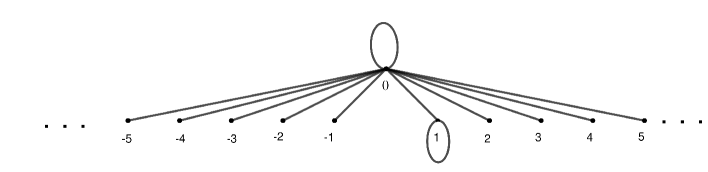
Figure 1. Countable graph $G$ with vertex set $\mathbb{Z}$ such that the loops are imposed at two vertices of the graph.

For $x\in S(y)$, $y\in V$, introduce new variables as $z_{i,x}=l_{xy}(i)$, then in case of $G$ (given in Fig.1), from (2.5) (see [6] and [1]) we obtain

$$\begin{cases}z_{1,x}=\lambda_{1}\prod_{y\in S(x)}{1+z_{1,y}\over 1+\sum_{j\in\mathbb{Z}_{0}}z_{j,y}},\\ z_{i,x}=\lambda_{i}\prod_{y\in S(x)}{1\over 1+\sum_{j\in\mathbb{Z}_{0}}z_{j,y}},\ \ i\in\mathbb{Z}_{0}\setminus\{1\}.\end{cases}$$ (2.6)

Remark 2.

Note that if we change the loop at vertex 1 to another arbitrary vertex (except vertex 0), we obtain a system of equations similar to (2.6), but in this case the notations may be slightly different. Therefore, it is sufficient to consider the case where there is a loop at vertex 1.

3. Translation-invariant measures for the model with two loops

The problem of the finding of the general form of solutions of the equation (2.6) seems to be very difficult. In this subsection, we consider translation-invariant solutions, i.e., $z_{x}=z=(z_{i})_{i\in\mathbb{Z}_{0}}$, with $z_{i}\in\mathbb{R}_{+}.$ In this case the equation (2.6) has the following form

$$\begin{cases}z_{1}=\lambda_{1}\left({1+z_{1}\over 1+\sum_{j\in\mathbb{Z}_{0}}z_{j}}\right)^{k},\\ z_{i}=\lambda_{i}\left({1\over 1+\sum_{j\in\mathbb{Z}_{0}}z_{j}}\right)^{k},\ \ i\in\mathbb{Z}_{0}\setminus\{1\}.\end{cases}$$ (3.1)

Here $\lambda_{i}>0,\ z_{i}>0$.

Lemma 1.

Let $k\geq 2$. If there is a positive solution $\{z_{j}\}_{j\in\mathbb{Z}_{0}}$ of the system of equations (3.1) for some sequence of parameters $\{\lambda_{j}\}_{j\in\mathbb{Z}_{0}}$ then series $\sum_{j\in\mathbb{Z}_{0}}z_{j}$ and $\sum_{j\in\mathbb{Z}_{0}}\lambda_{j}$ obtained respectively from $\{z_{i}\}_{i\in\mathbb{Z}_{0}}$ and $\{\lambda_{j}\}_{j\in\mathbb{Z}_{0}}$ converge.

Proof.

Let $\{z_{j}\}_{j\in\mathbb{Z}_{0}}$ be a solution of the system of equations (3.1). We assume that the series $\sum_{j\in\mathbb{Z}_{0}}z_{j}$ diverges. Then, since $z_{j}>0$, it is obvious that $\sum_{j\in\mathbb{Z}_{0}}z_{j}=+\infty$. Hence due to (3.1) we get $z_{i}=0,\ i\in\mathbb{Z}_{0}$, i.e., $\sum_{i\in\mathbb{Z}_{0}}z_{i}<+\infty.$ This is a contradiction. Therefore, under the conditions of lemma the series $\sum_{j\in\mathbb{Z}_{0}}z_{j}$ converges.

Let $\sum_{j\in\mathbb{Z}_{0}}z_{j}=A$. Then from (3.1) we obtain $A\left({1+A}\right)^{k}=\sum_{i\in\mathbb{Z}_{0}}\lambda_{i}+\lambda_{1}\left(\sum_{l=1}^{k}C_{k}^{l}z_{1}^{l}\right)$. Thus, $\sum_{i\in\mathbb{Z}_{0}}\lambda_{i}=A(1+A)^{k}-\lambda_{1}\left(\sum_{l=1}^{k}C_{k}^{l}z_{1}^{l}\right)$, i.e., the series $\sum_{i\in\mathbb{Z}_{0}}\lambda_{i}$ converges. Lemma is proved. ∎

By Lemma 1 it follows that there is no positive solution of the system of equations (3.1) for which the series $\sum_{j\in\mathbb{Z}_{0}}z_{j}$ and $\sum_{j\in\mathbb{Z}_{0}}\lambda_{j}$ diverge, i.e., these conditions are necessary for the existence of a solution (3.1).

Proposition 1.

Let $k=2$. If the series $\sum_{j\in\mathbb{Z}_{0}}\lambda_{j}$ obtained from a sequence of parameters $\{\lambda_{j}\}_{j\in\mathbb{Z}_{0}}$ converges then for the sequence $\{\lambda_{j}\}_{j\in\mathbb{Z}_{0}}$ there exists a unique positive solution $\{z_{j}\}_{j\in\mathbb{Z}_{0}}$ of the system of equations (3.1).

Proof.

Let the series $\sum_{j\in\mathbb{Z}_{0}}\lambda_{j}$ converge and its sum be $\sum_{j\in\mathbb{Z}_{0}}\lambda_{j}=\Lambda$. We will prove that for the sequence $\{\lambda_{j}\}_{j\in\mathbb{Z}_{0}}$ there is a unique solution of the system of equations (3.3). By Lemma 1 it follows that for the existence of a solution $\{z_{j}\}_{j\in\mathbb{Z}_{0}}$ of the system of equations (3.3) the convergence of the series $\sum_{j\in\mathbb{Z}_{0}}z_{j}$ is necessary.

Let $\sum_{j\in\mathbb{Z}_{0}}z_{j}=A$. Then due to (3.1) we get

$$\sum_{j\in\mathbb{Z}_{0}}z_{j}=\frac{\sum_{j\in\mathbb{Z}_{0}}\lambda_{j}+\lambda_{t}\left(2z_{t}+z_{t}^{2}\right)}{(1+A)^{2}}.$$

Hence

$$A(1+A)^{2}=\Lambda+\lambda_{1}\left(2z_{1}+z_{1}^{2}\right),\ A>0.$$ (3.2)

The first part of the system of equations (3.1) can be rewritten:

$$z_{1}(1+A)^{2}=\lambda_{1}\left(1+2z_{1}+z_{1}^{2}\right),$$ (3.3)

Solving (3.3) with respect to $z_{1}$, we have:

$$z_{1}^{(1,2)}=\frac{(1+A)^{2}-2\lambda_{1}\pm(1+A)\sqrt{(1+A)^{2}-4\lambda_{1}}}{2\lambda_{1}}$$

It is easy to see that if $(1+A)^{2}>4\lambda_{1}$ then $D>0$, $z_{1}^{(1,2)}>0$ and $z_{1}^{(1)}=1/z_{1}^{(2)}$.

On substituting $z_{1}=z_{1}^{(1)}$ in (3.2), we get

$$A(1+A)^{2}-\Lambda=\frac{(1+A)^{2}-2\lambda_{1}+(1+A)\sqrt{(1+A)^{2}-4\lambda_{1}}}{2}\cdot\frac{(1+A)^{2}+2\lambda_{1}+(1+A)\sqrt{(1+A)^{2}-4\lambda_{1}}}{2\lambda_{1}}$$

$$\Rightarrow\ \ A(1+A)^{2}-\Lambda=\frac{\left((1+A)^{2}+(1+A)\sqrt{(1+A)^{2}-4\lambda_{1}}\right)^{2}-4\lambda_{t}^{2}}{4\lambda_{1}}$$

$$\Rightarrow\ \ (1+A)^{4}+(1+A)^{3}\Big{(}\sqrt{(1+A)^{2}-4\lambda_{1}}-2\lambda_{1}\Big{)}+2\lambda_{1}(\Lambda-\lambda_{1})=0$$ (3.4)

Define

$$f(\lambda)=f(\lambda,x):=x^{4}+x^{3}\Big{(}\sqrt{x^{2}-4\lambda}-2\lambda\Big{)}+2\lambda(\Lambda-\lambda),\ \ \ \lambda\in\left(0,\frac{x^{2}}{4}\right].$$

In this case, the equation (3.4) can be written

$$f(\lambda,1+A)=0.$$ (3.5)

We calculate the first and second derivatives of the function $f(\lambda)$ with respect to $\lambda$:

$$f^{\prime}(\lambda)=\frac{-2x^{3}}{\sqrt{x^{2}-4\lambda}}+2\Lambda-2x^{3}-4\lambda\quad\ \ \ f^{\prime\prime}(\lambda)=-\frac{4x^{3}}{\sqrt{(x^{2}-4\lambda)^{3}}}-4<0.$$

It is easy to see that $f(\lambda)$ is a convex function, the derivative of $f^{\prime}(\lambda)$ exists in the interval $\lambda\in\left(0,\frac{x^{2}}{4}\right)$ and $f(0)=2x^{4}$. It follows that the function $f(\lambda)$ takes values smaller than $2x^{4}$ at most once. It means that the number of the solution of the equation $f(\lambda)=0$ is at most one.

On substituting $z_{1}=z_{1}^{(2)}$ in (3.2), we obtain

$$A(1+A)^{2}-\Lambda=\frac{(1+A)^{2}-2\lambda_{1}-(1+A)\sqrt{(1+A)^{2}-4\lambda_{1}}}{2}\cdot\frac{(1+A)^{2}+2\lambda_{1}-(1+A)\sqrt{(1+A)^{2}-4\lambda_{1}}}{2\lambda_{1}}$$

$$\Rightarrow\ \ A(1+A)^{2}-\Lambda=\frac{\left((1+A)^{2}-(1+A)\sqrt{(1+A)^{2}-4\lambda_{1}}\right)^{2}-4\lambda_{1}^{2}}{4\lambda_{1}}$$

$$\Rightarrow\ \ (1+A)^{4}-(1+A)^{3}\Big{(}\sqrt{(1+A)^{2}-4\lambda_{1}}+2\lambda_{1}\Big{)}+2\lambda_{1}(\Lambda-\lambda_{1})=0.$$ (3.6)

We introduce a new function

$$g(\lambda)=g(\lambda,x):=x^{4}-x^{3}\Big{(}\sqrt{x^{2}-4\lambda}+2\lambda\Big{)}+2\lambda(\Lambda-\lambda),\ \ \ \lambda\in\left(0,\frac{x^{2}}{4}\right].$$

In this case, the equation (3.6) can be written

$$g(\lambda,1+A)=0.$$ (3.7)

We calculate the first and second derivatives of the function $g(\lambda)$ with respect to $\lambda$:

$$g^{\prime}(\lambda)=\frac{-2x^{3}}{\sqrt{x^{2}-4\lambda}}+2\Lambda-2x^{3}-4\lambda\quad\ \ \ g^{\prime\prime}(\lambda)=\frac{4x^{3}}{\sqrt{(x^{2}-4\lambda)^{3}}}-4>0.$$

It is obvious that $g(\lambda)$ is a concave function, derivative $g^{\prime}(\lambda)$ exists in the interval $\lambda\in\left(0,\frac{x^{2}}{4}\right)$ and $g(0)=0$. It follows that the number of the positive solutions of the equation $g(\lambda)=0$ is at most one.

On the other hand, the function

$$\phi(\lambda):=f(\lambda)-g(\lambda)=2x^{3}\sqrt{x^{2}-4\lambda}$$

is decreasing with respect to $\lambda$ and $\phi(\frac{x^{2}}{4})=0$, i.e., $f(\frac{x^{2}}{4})=g(\frac{x^{2}}{4})$. As a result, the graph of the functions $f(\lambda)$ and $g(\lambda)$ together with the interval $[0;2x^{4}]$ of the $OY$ axis forms a closed line (see Fig.2).

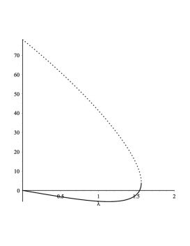
Figure 2. Graph functions $f(\lambda)$ (dotted line) and $g(\lambda)$ (solid line) for $x=2.5$ and $\Lambda=6$.

Then only one of the equations $f(\lambda)=0$ and $g(\lambda)=0$ would have a positive solution. If $f(\frac{x^{2}}{4})>0$ then the equation $g(\lambda)=0$ has a positive solution, if $f(\frac{x^{2}}{4})<0$ then the equation $f(\lambda)=0$ has a positive solution. Hence, there is a unique $x_{0}$ corresponding to each $\lambda$. Accordingly, there is a unique $A_{0}$ corresponding to each $\lambda$.

Therefore, the unique positive solution of the system of equations (3.1) is determined as follows:

If $f(\lambda)=0$ has a solution, then we take $z_{1}=z_{1}^{(1)}$ as a solution, if $g(\lambda)=0$ has a solution, then we take $z_{1}=z_{1}^{(2)}$ as a solution. The remaining coordinates are found as follows:

$$z_{i}={\lambda_{i}\over\left(1+A_{0}\right)^{2}},\ \ i\in\mathbb{Z}_{0}\setminus\{1\}.$$

∎

Remark 3.

We note that the solution $\{z_{j}\}_{j\in\mathbb{Z}_{0}}$ in Proposition 1 is normalisable because the convergence of series $\sum_{j\in\mathbb{Z}_{0}}z_{j}^{\frac{k+1}{k}}$ follows from the convergence of $\sum_{j\in\mathbb{Z}_{0}}z_{j}$. Then by Remark 1 the Gibbs measure (denoted by $\mu_{0}$) corresponding to this solution exists.

4. Markov chain corresponding to the obtained TIGM in Section 3

Below for the Gibbs measure $\mu_{0}$, we define a matrix $\mathbb{P}$ of transition probabilities. We will check the existence of a stationary distribution of the Markov chain corresponding to the measure $\mu_{0}$.

Consider the matrix $\mathbb{P}$ of transition probabilities corresponding to the measure $\mu_{0}$:

$$\mathbb{P}=\begin{pmatrix}\cdots&\vdots&\vdots&\vdots&\vdots&\vdots&\cdots\\ \cdots&p_{-2-2}&p_{-2-1}&p_{-20}&p_{-21}&p_{-22}&\cdots\\ \cdots&p_{-1-2}&p_{-1-1}&p_{-10}&p_{-11}&p_{-12}&\cdots\\ \cdots&p_{0-2}&p_{0-1}&p_{00}&p_{01}&p_{02}&\cdots\\ \cdots&p_{1-2}&p_{1-1}&p_{10}&p_{11}&p_{12}&\cdots\\ \cdots&p_{2-2}&p_{2-1}&p_{20}&p_{21}&p_{22}&\cdots\\ \cdots&\vdots&\vdots&\vdots&\vdots&\vdots&\cdots\end{pmatrix}.$$

Here (depending on solution $z=(z_{i})_{i\in\mathbb{Z}_{0}}$)

$$p_{\sigma(x)\sigma(y)}=\frac{a_{\sigma(x)\sigma(y)}\lambda_{\sigma{(y)}}z_{\sigma(y)}}{\sum_{\sigma(y)\in\Omega^{G}}{a_{\sigma(x)\sigma(y)}\lambda_{\sigma{(y)}}z_{\sigma(y)}}}\ \ \Rightarrow\ \ p_{ij}=\frac{a_{ij}\lambda_{j}z_{j}}{\sum_{l\in\mathbb{Z}}{a_{il}\lambda_{l}z_{l}}}.$$

For the considered model, $a_{11}=1$, $a_{i0}=1$, $a_{0j}=1$ and $a_{ij}=0$ for $i\in\mathbb{Z}_{0}$ and $j\in\mathbb{Z}_{0}$. Hence

$$p_{00}=\frac{\lambda_{0}z_{0}}{\lambda_{0}z_{0}+\sum_{l\in\mathbb{Z}_{0}}{\lambda_{l}z_{l}}}=\frac{1}{1+\sum_{l\in\mathbb{Z}_{0}}{\lambda^{\prime}_{l}z^{\prime}_{l}}},\ \ p_{11}=\frac{\lambda_{1}z_{1}}{\lambda_{0}z_{0}+\sum_{l\in\mathbb{Z}_{0}}{a_{1l}\lambda_{l}z_{l}}}=\frac{\lambda^{\prime}_{1}z^{\prime}_{1}}{1+\lambda^{\prime}_{1}z^{\prime}_{1}}$$

$$p_{01}=\frac{\lambda_{1}z_{1}}{\lambda_{0}z_{0}+\sum_{l\in\mathbb{Z}_{0}}{\lambda_{l}z_{l}}}=\frac{\lambda^{\prime}_{1}z^{\prime}_{1}}{1+\sum_{l\in\mathbb{Z}_{0}}{\lambda^{\prime}_{l}z^{\prime}_{l}}},\ \ p_{0i}=\frac{\lambda_{i}z^{\prime}_{i}}{1+\sum_{l\in\mathbb{Z}_{0}}{\lambda_{l}z^{\prime}_{l}}},$$

$$p_{10}=\frac{\lambda_{0}z_{0}}{\lambda_{0}z_{0}+\sum_{l\in\mathbb{Z}_{0}}{a_{1l}\lambda_{l}z_{l}}}=\frac{1}{1+\lambda^{\prime}_{1}z^{\prime}_{1}},\ \ p_{i0}=\frac{\lambda_{0}z_{0}}{\lambda_{0}z_{0}+\sum_{l\in\mathbb{Z}_{0}}{a_{il}\lambda_{l}z_{l}}}=1.$$

Therefore $\mathbb{P}$ has the following form (for $z_{0}=1$):

$$\mathbb{P}=\begin{pmatrix}\cdots&\vdots&\vdots&\vdots&\vdots&\vdots&\cdots\\ \cdots&0&0&1&0&0&\cdots\\ \cdots&0&0&1&0&0&\cdots\\ \cdots&\frac{\lambda_{-2}z_{-2}}{1+\sum_{l\in\mathbb{Z}_{0}}{\lambda_{l}z_{l}}}&\frac{\lambda_{-1}z_{-1}}{1+\sum_{l\in\mathbb{Z}_{0}}{\lambda_{l}z_{l}}}&\frac{1}{1+\sum_{l\in\mathbb{Z}_{0}}{\lambda_{l}z_{l}}}&\frac{\lambda_{1}z_{1}}{1+\sum_{l\in\mathbb{Z}_{0}}{\lambda_{l}z_{l}}}&\frac{\lambda_{2}z_{2}}{1+\sum_{l\in\mathbb{Z}_{0}}{\lambda_{l}z_{l}}}&\cdots\\ \cdots&0&0&\frac{1}{1+\lambda_{1}z_{1}}&\frac{\lambda_{1}z_{1}}{1+\lambda_{1}z_{1}}&0&\cdots\\ \cdots&0&0&1&0&0&\cdots\\ \cdots&\vdots&\vdots&\vdots&\vdots&\vdots&\cdots\end{pmatrix}$$

We consider the vector $X=(\cdots,x_{-2},x_{-1},x_{0},x_{1},x_{2},\cdots),\ \sum_{j\in\mathbb{Z}}{x_{j}}=1.$ If the system of equations $X\cdot\mathbb{P}=X$ has a solution then there exists a stationary distribution of the Markov chain corresponding to the measure $\mu_{0}$. So we solve the equation $X\cdot\mathbb{P}=X$. We have

$$X\cdot\mathbb{P}=\left(\cdots,\frac{x_{0}\lambda_{-2}z_{-2}}{1+\sum_{l\in\mathbb{Z}_{0}}{\lambda_{l}z_{l}}},\frac{x_{0}\lambda_{-1}z_{-1}}{1+\sum_{l\in\mathbb{Z}_{0}}{\lambda_{l}z_{l}}},p_{00},\frac{x_{0}\lambda_{1}z_{1}}{1+\sum_{l\in\mathbb{Z}_{0}}{\lambda_{l}z_{l}}}+\frac{x_{1}\lambda_{1}z_{1}}{1+\lambda_{1}z_{1}},\frac{x_{0}\lambda_{2}z_{2}}{1+\sum_{l\in\mathbb{Z}_{0}}{\lambda_{l}z_{l}}},\cdots\right),$$

where

$$p_{00}=1-\frac{x_{0}\sum_{l\in\mathbb{Z}_{0}}{\lambda_{l}z_{l}}}{1+\sum_{l\in\mathbb{Z}_{0}}{\lambda_{l}z_{l}}}-\frac{x_{1}\lambda_{1}z_{1}}{1+\lambda_{1}z_{1}}.$$

From the equality $X\cdot\mathbb{P}=X$ we get

$$x_{0}=1-\frac{x_{0}\sum_{l\in\mathbb{Z}_{0}}{\lambda_{l}z_{l}}}{1+\sum_{l\in\mathbb{Z}_{0}}{\lambda_{l}z_{l}}}-\frac{x_{1}\lambda_{1}z_{1}}{1+\lambda_{1}z_{1}},\ x_{1}=\ \frac{x_{0}\lambda_{1}z_{1}}{1+\sum_{l\in\mathbb{Z}_{0}}{\lambda_{l}z_{l}}}+\frac{x_{1}\lambda_{1}z_{1}}{1+\lambda_{1}z_{1}},\ \ x_{j}=\frac{x_{0}\lambda_{j}z_{j}}{1+\sum_{l\in\mathbb{Z}_{0}}{\lambda_{l}z_{l}}},$$ (4.1)

where $j\in\mathbb{Z}_{0}\setminus\{1\}.$

From the equality of (4.1) we find $x_{0}$ and $x_{1}$:

$$x_{0}=\frac{1+\sum_{l\in\mathbb{Z}_{0}}\lambda_{l}z_{l}}{1+\lambda_{1}^{2}z_{1}^{2}+2\sum_{l\in\mathbb{Z}_{0}}\lambda_{l}z_{l}},\ \ x_{1}=\frac{\lambda_{1}^{2}z_{1}^{2}+\lambda_{1}z_{1}}{1+\lambda_{1}^{2}z_{1}^{2}+2\sum_{l\in\mathbb{Z}_{0}}\lambda_{l}z_{l}}.$$

Using the expression for $x_{0}$ from the third equality of (4.1) we find $x_{j}$, $j\in\mathbb{Z}_{0}\setminus\{1\}$:

$$x_{j}=\frac{\lambda_{j}z_{j}}{1+\lambda_{1}^{2}z_{1}^{2}+2\sum_{l\in\mathbb{Z}_{0}}\lambda_{l}z_{l}}.$$

It is easy to see that the obtained vector is stochastic:

$$\sum_{j\in\mathbb{Z}}{x_{j}}=\frac{1+\sum_{l\in\mathbb{Z}_{0}}\lambda_{l}z_{l}}{1+\lambda_{1}^{2}z_{1}^{2}+2\sum_{l\in\mathbb{Z}_{0}}\lambda_{l}z_{l}}+\frac{\lambda_{1}^{2}z_{1}^{2}+\lambda_{1}z_{1}}{1+\lambda_{1}^{2}z_{1}^{2}+2\sum_{l\in\mathbb{Z}_{0}}\lambda_{l}z_{l}}+\frac{\sum_{l\in\mathbb{Z}_{0}\setminus\{1\}}\lambda_{l}z_{l}}{1+\lambda_{1}^{2}z_{1}^{2}+2\sum_{l\in\mathbb{Z}_{0}}\lambda_{l}z_{l}}=1.$$

Hence there exists a stationary distribution of the Markov chain corresponding to the measure $\mu_{0}$.

Due to the uniqueness of the stationary distribution from Theorem 2 in [15], (p.612) we get

Corollary 1.

In the set of states $\mathbb{Z}$ of a Markov chain with the transition probabilities matrix $\mathbb{P}$, there is exactly one positive recurrent class of essential communicating states (for definitions, see Chapter VIII in [15]).

Summarizing, we have

Theorem 1.

Let $k=2$. Then for the HC model with a countable set of states (corresponding to the graph plotted in Fig.1) the following statements are true:

• If the series $\sum_{j\in\mathbb{Z}_{0}}\lambda_{j}$ obtained from a sequence of parameters $\{\lambda_{j}\}_{j\in\mathbb{Z}_{0}}$ converges then there exists a unique translation-invariant Gibbs measure.

• If the series $\sum_{j\in\mathbb{Z}_{0}}\lambda_{j}$ diverges there is no translation-invariant Gibbs measure.

5. Translation-invariant measures for the model with three loops

We consider the graph $G$ with $a_{i0}=1$ for any $i\in\mathbb{Z}$, $a_{11}=1$, $a_{22}=1$ and $a_{im}=0$ otherwise (see Fig.3).

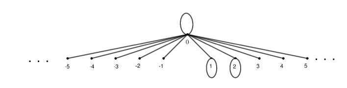
Figure 3. Countable graph $G$ with vertex set $\mathbb{Z}$ such that the loops are imposed at three vertices of the graph.

For $x\in S(y)$, $y\in V$, introduce new variables as $z_{i,x}=l_{xy}(i)$, then in case of $G$ (given in Fig.3), from (2.5) we obtain

$$\begin{cases}z_{1,x}=\lambda_{1}\prod_{y\in S(x)}{1+z_{1,y}\over 1+\sum_{j\in\mathbb{Z}_{0}}z_{j,y}},\\ z_{2,x}=\lambda_{2}\prod_{y\in S(x)}{1+z_{2,y}\over 1+\sum_{j\in\mathbb{Z}_{0}}z_{j,y}},\\ z_{i,x}=\lambda_{i}\prod_{y\in S(x)}{1\over 1+\sum_{j\in\mathbb{Z}_{0}}z_{j,y}},\ \ i\in\mathbb{Z}_{0}\setminus\{1,2\}.\end{cases}$$ (5.1)

Remark 4.

As mentioned in Remark 2, in general, the location of the loops in the vertices (except vertex 0) of the graph does not matter.

In this section, we consider translation invariant solutions of (5.1), i.e., $z_{x}=z=(z_{i})_{i\in\mathbb{Z}_{0}}$, with $z_{i}\in\mathbb{R}_{+}.$ In this case the equation (5.1) has the following form

$$\begin{cases}z_{1}=\lambda_{1}\left({1+z_{1}\over 1+\sum_{j\in\mathbb{Z}_{0}}z_{j}}\right)^{k},\\ z_{2}=\lambda_{2}\left({1+z_{2}\over 1+\sum_{j\in\mathbb{Z}_{0}}z_{j}}\right)^{k},\\ z_{i}=\lambda_{i}\left({1\over 1+\sum_{j\in\mathbb{Z}_{0}}z_{j}}\right)^{k},\ \ i\in\mathbb{Z}_{0}\setminus\{1,2\}.\end{cases}$$ (5.2)

Here $\lambda_{i}>0,\ z_{i}>0$.

Lemma 2.

Let $k\geq 1$. If there is a positive solution $\{z_{j}\}_{j\in\mathbb{Z}_{0}}$ of the system of equations (5.2) for some sequence of parameters $\{\lambda_{j}\}_{j\in\mathbb{Z}_{0}}$ then series $\sum_{j\in\mathbb{Z}_{0}}z_{j}$ and $\sum_{j\in\mathbb{Z}_{0}}\lambda_{j}$ obtained respectively from $\{z_{i}\}_{i\in\mathbb{Z}_{0}}$ and $\{\lambda_{j}\}_{j\in\mathbb{Z}_{0}}$ converge.

Proof.

The proof runs applying the very similar arguments as in Lemma 1. In this case, we have $\sum_{i\in\mathbb{Z}_{0}}\lambda_{i}=A(1+A)^{k}-\lambda_{1}\left(\sum_{l=1}^{k}C_{k}^{l}z_{1}^{l}\right)-\lambda_{2}\left(\sum_{l=1}^{k}C_{k}^{l}z_{2}^{l}\right)$. ∎

By Lemma 2 it follows that there is no positive solution of the system of equations (5.2) for which the series $\sum_{j\in\mathbb{Z}_{0}}z_{j}$ and $\sum_{j\in\mathbb{Z}_{0}}\lambda_{j}$ diverge, i.e., these conditions are necessary for the existence of a solution (5.2).

First, let us consider the first and second parts of the system of equations (5.2):

$$\begin{cases}z_{1}=\lambda_{1}\left({1+z_{1}\over 1+\sum_{j\in\mathbb{Z}_{0}}z_{j}}\right)^{k},\\ z_{2}=\lambda_{2}\left({1+z_{2}\over 1+\sum_{j\in\mathbb{Z}_{0}}z_{j}}\right)^{k},\\ \end{cases}$$ (5.3)

In our further studies, it is very difficult to analyze the system of equations (5.3) in the general case. Therefore, in (5.3) we assume $\lambda=\lambda_{1}=\lambda_{2}$ and write the system of equations (5.3) as follows:

$$\begin{cases}z_{1}=\lambda\left({1+z_{1}\over 1+\sum_{j\in\mathbb{Z}_{0}}z_{j}}\right)^{k},\\ z_{2}=\lambda\left({1+z_{2}\over 1+\sum_{j\in\mathbb{Z}_{0}}z_{j}}\right)^{k}.\\ \end{cases}$$ (5.4)

Let $\Lambda_{1}=\frac{2\lambda^{2}+36\lambda-81}{\lambda}$ and $\Lambda_{2}=\frac{1}{1024}\left((18\lambda^{2}+64\lambda)\sqrt{9\lambda^{2}+32\lambda}+54\lambda^{3}+288\lambda^{2}+2304\lambda\right)$.

Proposition 2.

Let $k=2$ and the series $\sum_{j\in\mathbb{Z}_{0}}\lambda_{j}$ obtained from the sequence of parameters $\{\lambda_{j}\}_{j\in\mathbb{Z}_{0}}$ converge and its sum $\Lambda=\sum_{j\in\mathbb{Z}_{0}}\lambda_{j}$. Then the system of equations (5.2):

1) For $\lambda\leq\frac{49}{9}$ and $\Lambda\geq\Lambda_{1}$ has a unique solution;

2) For $\lambda\leq\frac{49}{9}$ and $\Lambda<\Lambda_{1}$ has three solutions;

3) For $\lambda>\frac{49}{9}$ and $\Lambda\leq\Lambda_{1}$ has three solutions;

4) For $\lambda>\frac{49}{9}$ and $\Lambda_{1}<\Lambda<\Lambda_{2}$ has five solutions;

5) For $\lambda>\frac{49}{9}$ and $\Lambda=\Lambda_{2}$ has three solutions;

6) For $\lambda>\frac{49}{9}$ and $\Lambda>\Lambda_{2}$ has a unique solution

Proof.

The proof will be given for the cases $z_{1}=z_{2}$ and $z_{1}\neq z_{2}$, separately.

Case $z_{1}=z_{2}$. Let the series $\sum_{j\in\mathbb{Z}_{0}}\lambda_{j}$ converge and its sum be $\sum_{j\in\mathbb{Z}_{0}}\lambda_{j}=\Lambda$. It follows from Lemma 2 that for the existence of a solution $\{z_{j}\}_{j\in\mathbb{Z}_{0}}$ of the system of equations (5.2), the series $\sum_{j\in\mathbb{Z}_{0}}z_{j}$ converges .

Let $\sum_{j\in\mathbb{Z}_{0}}z_{j}=A$. Then due to (5.2) we get

$$\sum_{j\in\mathbb{Z}_{0}}z_{j}=\frac{\sum_{j\in\mathbb{Z}_{0}}\lambda_{j}+2\lambda\left(2z_{1}+z_{1}^{2}\right)}{(1+A)^{2}},$$

i.e.,

$$A(1+A)^{2}=\Lambda+2\lambda z_{1}\left(2+z_{1}\right),\ A>0.$$ (5.5)

From the first and second parts of the system of equations (5.2), the following can be rewritten:

$$z_{1}(1+A)^{2}=\lambda\left(1+2z_{1}+z_{1}^{2}\right),\ \ \$$ (5.6)

Solving (5.6) with respect to $z_{1}$, we have:

$$z_{1}^{(1,2)}=\frac{(1+A)^{2}-2\lambda\pm(1+A)\sqrt{(1+A)^{2}-4\lambda}}{2\lambda}$$

It is easy to see that if $(1+A)^{2}>4\lambda$ then $D>0$, $z_{1}^{(1,2)}>0$ and $z_{1}^{(1)}=1/z_{1}^{(2)}$.

On substituting $z_{1}=z_{2}=z_{1}^{(1)}$ into (5.5), we get:

$$A(1+A)^{2}-\Lambda=\left((1+A)^{2}-2\lambda+(1+A)\sqrt{(1+A)^{2}-4\lambda}\right)\cdot\frac{(1+A)^{2}+2\lambda+(1+A)\sqrt{(1+A)^{2}-4\lambda}}{2\lambda}$$

$$\Rightarrow\ \ (1+A)^{4}+(1+A)^{3}\sqrt{(1+A)^{2}-4\lambda}-\lambda(1+A)^{2}(2+A)+\lambda(\Lambda-2\lambda)=0$$ (5.7)

Consider the following function:

$$h(\lambda)=h(\lambda,x):=(1+x)^{4}+(1+x)^{3}\sqrt{(1+x)^{2}-4\lambda}-\lambda(1+x)^{2}(2+x)+\lambda(\Lambda-2\lambda),\ \ \ \lambda\in\left(0,\frac{(1+x)^{2}}{4}\right].$$

In this case, the equation (5.7) can be written

$$h(\lambda,A)=0.$$ (5.8)

We calculate the first and second derivatives of the function $h(\lambda)$ with respect to $\lambda$:

$$h^{\prime}(\lambda)=-(x+1)^{2}(x+2)-\frac{2(x+1)^{3}}{\sqrt{(x+1)^{2}-4\lambda}}-4\lambda+\Lambda\quad\ \ \ h^{\prime\prime}(\lambda)=-\frac{4(x+1)^{3}}{\sqrt{((x+1)^{2}-4\lambda)^{3}}}-4<0$$

It is easy to see that $h(\lambda)$ is a convex function, $h^{\prime}(\lambda)$ exists in the interval $\lambda\in\left(0,\frac{(1+x)^{2}}{4}\right)$ and $h(0)=2(x+1)^{4}$. It follows that the function $h(\lambda)$ takes values smaller than $2(x+1)^{4}$ at most once. Therefore, the number of the solution of the equation $h(\lambda)=0$ is at most one.

Let us put $z_{1}=z_{2}=z_{1}^{(2)}$ in (5.5). In that case:

$$A(1+A)^{2}-\Lambda=\left((1+A)^{2}-2\lambda-(1+A)\sqrt{(1+A)^{2}-4\lambda}\right)\cdot\frac{(1+A)^{2}+2\lambda-(1+A)\sqrt{(1+A)^{2}-4\lambda}}{2\lambda}$$

$$\Rightarrow\ \ (1+A)^{4}-(1+A)^{3}\sqrt{(1+A)^{2}-4\lambda}-\lambda(1+A)^{2}(2+A)+\lambda(\Lambda-2\lambda)=0$$ (5.9)

Consider the following function:

$$\delta(\lambda)=(1+x)^{4}-(1+x)^{3}\sqrt{(1+x)^{2}-4\lambda}-\lambda(1+x)^{2}(2+x)+\lambda(\Lambda-2\lambda),\ \ \ \ \lambda\in\left(0,\frac{(1+x)^{2}}{4}\right].$$

In this case, the equation (5.9) can be written

$$\delta(\lambda,A)=0.$$ (5.10)

We calculate the first and second derivatives of the function $\delta(\lambda)$ with respect to $\lambda$:

$$\delta^{\prime}(\lambda)=-(x+1)^{2}(x+2)+\frac{2(x+1)^{3}}{\sqrt{(x+1)^{2}-4\lambda}}-4\lambda+\Lambda\quad\ \ \ \delta^{\prime\prime}(\lambda)=\frac{4(x+1)^{3}}{\sqrt{((x+1)^{2}-4\lambda)^{3}}}-4<0.$$

It is obvious that $\delta(\lambda)$ is a concave function, $\delta^{\prime}(\lambda)$ exists in $\lambda\in\left(0,\frac{(x+1)^{2}}{4}\right)$ and $\delta(0)=0$. Therefore, the equation $\delta(\lambda)=0$ has at most one positive solution.

On the other hand, the function

$$\psi(\lambda):=h(\lambda)-\delta(\lambda)=2(x+1)^{3}\sqrt{(x+1)^{2}-4\lambda}$$

is decreasing with respect to $\lambda$ and $\psi\Big{(}\frac{(x+1)^{2}}{4}\Big{)}=$0, i.e., $h\Big{(}\frac{(x+1)^{2}}{4}\Big{)}=\delta\Big{(}\frac{(x+1)^{2}}{4}\Big{)}$. As a result, the graph of the functions $h(\lambda)$ and $\delta(\lambda)$ together with the interval $[0;2(x+1)^{4}]$ of the $OY$ axis forms a closed line (see Fig.4 ). Then only one of the equations $h(\lambda)=0$ and $\delta(\lambda)=0$ would have a positive solution. If $h\Big{(}\frac{(x+1)^{2}}{4}\Big{)}>0$ then the equation $\delta(\lambda)=0$ has a positive solution, if $h\Big{(}\frac{(x+1)^{2}}{4}\Big{)}<0$ then the equation $h(\lambda)=0$ has a positive solution. Hence, there is a unique $x_{0}$ corresponding to each $\lambda$. Accordingly, there is a unique $A_{0}$ corresponding to each $\lambda$.

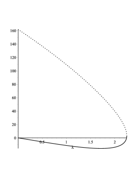
Figure 4. Graph functions $h(\lambda)$ (dotted line) and $\delta(\lambda)$ (solid line) for $x=2$ and $\Lambda=10$.

Then the unique positive solution of the system of equations (5.2) is determined as follows:

If the equation $h(\lambda)=0$ has a solution then we take $z_{1}=z_{2}=z_{1}^{(1)}$ as a solution, if the equation $\delta(\lambda)=0$ has a solution then we take $z_{1}=z_{2}=z_{1}^{(2)}$ as a solution. The remaining coordinates are found as follows:

$$z_{i}={\lambda_{i}\over\left(1+A_{0}\right)^{2}},\ \ i\in\mathbb{Z}_{0}\setminus\{1,2\}.$$

Case $z_{1}\neq z_{2}$. Let the series $\sum_{j\in\mathbb{Z}_{0}}\lambda_{j}$ converge and its sum be $\sum_{j\in\mathbb{Z}_{0}}\lambda_{j}=\Lambda$. It follows from Lemma 2 that for the existence of a solution $\{z_{j}\}_{j\in\mathbb{Z}_{0}}$ of the system of equations (5.2), the series $\sum_{j\in\mathbb{Z}_{0}}z_{j}$ converges .

Let $\sum_{j\in\mathbb{Z}_{0}}z_{j}=A$. Then due to (5.2) we get

$$\sum_{j\in\mathbb{Z}_{0}}z_{j}=\frac{\sum_{j\in\mathbb{Z}_{0}}\lambda_{j}+\lambda\left(2z_{1}+z_{1}^{2}+2z_{2}+z_{2}^{2}\right)}{(1+A)^{2}},$$

i.e.,

$$A(1+A)^{2}=\Lambda+\lambda\left(2z_{1}+z_{1}^{2}+2z_{2}+z_{2}^{2}\right),\ A>0.$$ (5.11)

The first and second parts of the system of equations (5.2) can be rewritten:

$$z_{1}(1+A)^{2}=\lambda\left(1+2z_{1}+z_{1}^{2}\right),\ \ \ z_{2}(1+A)^{2}=\lambda\left(1+2z_{2}+z_{2}^{2}\right).$$ (5.12)

Solving (5.12) with respect to $z_{1}$ (resp. $z_{2}$):

$$z^{(1,2)}=\frac{(1+A)^{2}-2\lambda\pm(1+A)\sqrt{(1+A)^{2}-4\lambda}}{2\lambda}$$

It is easy to see that if $(1+A)^{2}>4\lambda$ then $D>0$, $z_{t}^{(1,2)}>0$ and $z^{(1)}=1/z^{(2)}$.

On substituting $z_{1}=z^{(1)}$ and $z_{2}=z^{(2)}$ into (5.11), we obtain

$$A(1+A)^{2}=\Lambda+\frac{1}{\lambda}\Big{(}(1+A)^{4}-2\lambda(1+A)^{2}-2\lambda^{2}\Big{)}\ \ \ \Rightarrow$$

$$(1+A)^{4}-\lambda(A+2)(1+A)^{2}+\lambda\Lambda-2\lambda^{2}=0$$ (5.13)

Consider the following function:

$$q(x)=q(x,\lambda):=(1+x)^{4}-\lambda(x+2)(1+x)^{2}+\lambda\Lambda-2\lambda^{2}.$$

We calculate the first derivative of the function $q(x)$ with respect to $x$:

$$q^{\prime}(x)=4x^{3}+(12-3\lambda)x^{2}+(12-8\lambda)x+4-5\lambda.$$

The solutions of $q^{\prime}(x)=0$ are

$$x_{1}=-1,\ \ x_{2}=\frac{3\lambda-8-\sqrt{9\lambda^{2}+32\lambda}}{8},\ \ \ x_{3}=\frac{3\lambda-8+\sqrt{9\lambda^{2}+32\lambda}}{8}$$

Since $(A+1)^{2}>4\lambda$, it suffices to check the function $q(x)$ in the interval $x>2\sqrt{\lambda}-1$.

If $\lambda>0$ then $x_{2}<0$, and if $\lambda>\frac{49}{9}$, then $x_{3}>2\sqrt{\lambda}-1$. Therefore, if $\lambda>\frac{49}{9}$ the function $q(x)$ is increasing for $x>x_{3}$, and decreasing for $2\sqrt{\lambda}-1<x<x_{3}$.

$(i)$ Let $\lambda\leq\frac{49}{9}$. Then the function $q(x)$ is increasing for $x>2\sqrt{\lambda}-1$. It is easy to verify that if $\Lambda<\Lambda_{1}$ then the equation $q(x)=0$ has a unique positive solution for $x>2\sqrt{\lambda}-1$, i.e.,

$$q\left(2\sqrt{\lambda}-1\right)=\lambda\Lambda+10\lambda^{2}-8\lambda^{5/2}<0,\quad\Rightarrow\quad\Lambda<\Lambda_{1}=8\lambda^{3/2}-10\lambda.$$

If $\Lambda\geq\Lambda_{1}$ then the equation $q(x)=0$ does not have a positive solution in the interval $x>2\sqrt{\lambda}-1$, i.e.,

$$q\left(2\sqrt{\lambda}-1\right)=\lambda\Lambda+10\lambda^{2}-8\lambda^{5/2}\geq 0,\quad\Rightarrow\quad\Lambda\geq\Lambda_{1}=8\lambda^{3/2}-10\lambda.$$

$(ii)$ Let $\lambda>\frac{49}{9}$. Then the function $q(x)$ is increasing for $x>x_{3}$, and decreasing for $2\sqrt{\lambda}-1<x<x_{3}$.

At the point $x=x_{3}$, it reaches its local minimum in the interval $x>2\sqrt{\lambda}-1$, and

$$q(x_{3})=-\frac{\lambda}{512}\left((9\lambda^{2}+32\lambda)\sqrt{9\lambda^{2}+32\lambda}+27\lambda^{3}+144\lambda^{2}-512\Lambda+1152\lambda\right)$$

On the other hand,

$$q\left(2\sqrt{\lambda}-1\right)=\lambda\Lambda+10\lambda^{2}-8\lambda^{5/2},\ \ q(\infty)=\infty.$$

Assume that $\Lambda_{1}=8\lambda^{3/2}-10\lambda$ and $\Lambda_{2}=\frac{1}{512}\left((9\lambda^{2}+32\lambda)\sqrt{9\lambda^{2}+32\lambda}+27\lambda^{3}+144\lambda^{2}+1152\lambda\right)$ bo’lsin. Obviously, if $\lambda>\frac{49}{9}$, then $\Lambda_{1}<\Lambda_{2}$. Then we have the following assertions:

$(i)$ If $q\left(2\sqrt{\lambda}-1\right)\leq 0$ and $q(x_{3})<0$, i.e. $\Lambda\leq\Lambda_{1}$, then the equation $q(x)=0$ has a unique positive solution for $x>2\sqrt{\lambda}-1$;

$(ii)$ If $q\left(2\sqrt{\lambda}-1\right)>0$ and $q(x_{3})<0$, i.e. $\Lambda_{1}<\Lambda<\Lambda_{2}$, then the equation $q(x)=0$ has 2 positive solutions for $x>2\sqrt{\lambda}-1$;

$(iii)$ If $q\left(2\sqrt{\lambda}-1\right)>0$ and $q(x_{3})=0$, i.e. $\Lambda=\Lambda_{2}$, then $q(x)=0$ has a unique positive solution for $x>2\sqrt{\lambda}-1$.

$(iv)$ If $q\left(2\sqrt{\lambda}-1\right)>0$ and $q(x_{3})>0$, i.e. $\Lambda>\Lambda_{2}$, then the equation $q(x)=0$ does not have a positive solution for $x>2\sqrt{\lambda}-1$.

Suppose that the solutions of the equation $q(x)=0$ are $A_{1}$ and $A_{2}$. Then the solutions of the system of equations (5.2) are:

$$z_{1}=\frac{(1+A_{1})^{2}-2\lambda+(1+A_{1})\sqrt{(1+A_{1})^{2}-4\lambda}}{2\lambda},\ \ z_{2}=\frac{1}{z_{1}},\ \ z_{i}={\lambda_{i}\over\left(1+A_{1}\right)^{2}},\ \ i\in\mathbb{Z}_{0}\setminus\{1,2\}.$$

$$z_{1}=\frac{(1+A_{2})^{2}-2\lambda+(1+A_{2})\sqrt{(1+A_{2})^{2}-4\lambda}}{2\lambda},\ \ z_{2}=\frac{1}{z_{1}},\ \ z_{i}={\lambda_{i}\over\left(1+A_{2}\right)^{2}},\ \ i\in\mathbb{Z}_{0}\setminus\{1,2\}.$$

Applying above process to $z_{1}=z^{(2)}$ and $z_{2}=z^{(1)}$, respectively, we obtain:

suppose that the solutions of the equation $q(x)=0$ are $A_{1}$ and $A_{2}$. Then the solutions of the system of equations (5.2) are:

$$z_{1}=\frac{(1+A_{1})^{2}-2\lambda-(1+A_{1})\sqrt{(1+A_{1})^{2}-4\lambda}}{2\lambda},\ \ z_{2}=\frac{1}{z_{1}},\ \ z_{i}={\lambda_{i}\over\left(1+A_{1}\right)^{2}},\ \ i\in\mathbb{Z}_{0}\setminus\{1,2\}.$$

$$z_{1}=\frac{(1+A_{2})^{2}-2\lambda-(1+A_{2})\sqrt{(1+A_{2})^{2}-4\lambda}}{2\lambda},\ \ z_{2}=\frac{1}{z_{1}},\ \ z_{i}={\lambda_{i}\over\left(1+A_{2}\right)^{2}},\ \ i\in\mathbb{Z}_{0}\setminus\{1,2\}.$$

∎

Remark 5.

We note that the solution $\{z_{j}\}_{j\in\mathbb{Z}_{0}}$ in Proposition 2 is normalisable because the convergence of series $\sum_{j\in\mathbb{Z}_{0}}z_{j}^{\frac{k+1}{k}}$ follows from the convergence of $\sum_{j\in\mathbb{Z}_{0}}z_{j}$. Then by Remark 1 the Gibbs measure (denoted by $\mu_{i}$, $i=1...5$) corresponding to this solution exists.

6. Markov chain corresponding to the obtained TIGMs in Section 5

For the Gibbs measure $\mu_{i}$, $i=1...5$ we define a matrix $\mathbb{P}_{1}$ of transition probabilities. We construct the matrix $\mathbb{P}_{1}$ using the very similar arguments as in Section 4.

For the considered model, $a_{11}=1$, $a_{22}$=1, $a_{i0}=1$, $a_{0j}=1$ and $a_{ij}=0$ for $i\in\mathbb{Z}_{0}$ and $j\in\mathbb{Z}_{0}$. Hence

$$p_{00}=\frac{1}{1+\sum_{l\in\mathbb{Z}_{0}}{\lambda^{\prime}_{l}z^{\prime}_{l}}},\ \ p_{11}=\frac{\lambda^{\prime}_{1}z^{\prime}_{1}}{1+\lambda^{\prime}_{1}z^{\prime}_{1}},\ \ p_{22}=\frac{\lambda^{\prime}_{2}z^{\prime}_{2}}{1+\lambda^{\prime}_{2}z^{\prime}_{2}},\ \ p_{01}=\frac{\lambda^{\prime}_{1}z^{\prime}_{1}}{1+\sum_{l\in\mathbb{Z}_{0}}{\lambda^{\prime}_{l}z^{\prime}_{l}}},$$

$$p_{0i}=\frac{\lambda_{i}z^{\prime}_{i}}{1+\sum_{l\in\mathbb{Z}_{0}}{\lambda_{l}z^{\prime}_{l}}},\ \ p_{10}=\frac{1}{1+\lambda^{\prime}_{1}z^{\prime}_{1}},\ \ p_{20}=\frac{1}{1+\lambda^{\prime}_{2}z^{\prime}_{2}},\ \ p_{i0}=1.$$

Therefore $\mathbb{P}_{1}$ has the following form:

$$\mathbb{P}_{1}=\begin{pmatrix}\cdots&\vdots&\vdots&\vdots&\vdots&\vdots&\cdots\\ \cdots&0&0&1&0&0&\cdots\\ \cdots&0&0&1&0&0&\cdots\\ \cdots&\frac{\lambda_{-2}z_{-2}}{1+\sum_{l\in\mathbb{Z}_{0}}{\lambda_{l}z_{l}}}&\frac{\lambda_{-1}z_{-1}}{1+\sum_{l\in\mathbb{Z}_{0}}{\lambda_{l}z_{l}}}&\frac{1}{1+\sum_{l\in\mathbb{Z}_{0}}{\lambda_{l}z_{l}}}&\frac{\lambda_{1}z_{1}}{1+\sum_{l\in\mathbb{Z}_{0}}{\lambda_{l}z_{l}}}&\frac{\lambda_{2}z_{2}}{1+\sum_{l\in\mathbb{Z}_{0}}{\lambda_{l}z_{l}}}&\cdots\\ \cdots&0&0&\frac{1}{1+\lambda_{1}z_{1}}&\frac{\lambda_{1}z_{1}}{1+\lambda_{1}z_{1}}&0&\cdots\\ \cdots&0&0&\frac{1}{1+\lambda_{2}z_{2}}&0&\frac{\lambda_{2}z_{2}}{1+\lambda_{2}z_{2}}&\cdots\\ \cdots&0&0&1&0&0&\cdots\\ \cdots&\vdots&\vdots&\vdots&\vdots&\vdots&\cdots\end{pmatrix}$$

We consider the vector $X=(\cdots,x_{-2},x_{-1},x_{0},x_{1},x_{2},\cdots),\ \sum_{j\in\mathbb{Z}}{x_{j}}=1.$ We solve the equation $X\cdot\mathbb{P}_{1}=X$. We have

$$X\cdot\mathbb{P}_{1}=\left(\cdots,\frac{x_{0}\lambda_{-2}z_{-2}}{1+\sum_{l\in\mathbb{Z}_{0}}{\lambda_{l}z_{l}}},\frac{x_{0}\lambda_{-1}z_{-1}}{1+\sum_{l\in\mathbb{Z}_{0}}{\lambda_{l}z_{l}}},p_{0},p_{1},p_{2},\frac{x_{0}\lambda_{3}z_{3}}{1+\sum_{l\in\mathbb{Z}_{0}}{\lambda_{l}z_{l}}},\cdots\right),$$

where

$$p_{0}=1-\frac{x_{0}\sum_{l\in\mathbb{Z}_{0}}{\lambda_{l}z_{l}}}{1+\sum_{l\in\mathbb{Z}_{0}}{\lambda_{l}z_{l}}}-\frac{x_{1}\lambda_{1}z_{1}}{1+\lambda_{1}z_{1}}-\frac{x_{2}\lambda_{2}z_{2}}{1+\lambda_{2}z_{2}}$$

$$p_{1}=\frac{x_{0}\lambda_{1}z_{1}}{1+\sum_{l\in\mathbb{Z}_{0}}{\lambda_{l}z_{l}}}+\frac{x_{1}\lambda_{1}z_{1}}{1+\lambda_{1}z_{1}},\ \ \ p_{2}=\frac{x_{0}\lambda_{1}z_{1}}{1+\sum_{l\in\mathbb{Z}_{0}}{\lambda_{l}z_{l}}}+\frac{x_{2}\lambda_{2}z_{2}}{1+\lambda_{2}z_{2}}$$

From the equality $X\cdot\mathbb{P}_{1}=X$ we get

$$x_{0}=1-\frac{x_{0}\sum_{l\in\mathbb{Z}_{0}}{\lambda_{l}z_{l}}}{1+\sum_{l\in\mathbb{Z}_{0}}{\lambda_{l}z_{l}}}-\frac{x_{1}\lambda_{1}z_{1}}{1+\lambda_{1}z_{1}}-\frac{x_{2}\lambda_{2}z_{2}}{1+\lambda_{2}z_{2}},\ \ x_{1}=\frac{x_{0}\lambda_{1}z_{1}}{1+\sum_{l\in\mathbb{Z}_{0}}{\lambda_{l}z_{l}}}+\frac{x_{1}\lambda_{1}z_{1}}{1+\lambda_{1}z_{1}},$$

$$x_{2}=\frac{x_{0}\lambda_{1}z_{1}}{1+\sum_{l\in\mathbb{Z}_{0}}{\lambda_{l}z_{l}}}+\frac{x_{2}\lambda_{2}z_{2}}{1+\lambda_{2}z_{2}},\ \ x_{j}=\frac{x_{0}\lambda_{j}z_{j}}{1+\sum_{l\in\mathbb{Z}_{0}}{\lambda_{l}z_{l}}},$$ (6.1)

where $j\in\mathbb{Z}_{0}\setminus\{1,2\}.$

From the equality of (6.1) we find $x_{0}$, $x_{1}$ and $x_{2}$:

$$x_{0}=\frac{1+\sum_{l\in\mathbb{Z}_{0}}\lambda_{l}z_{l}}{1+\lambda_{1}^{2}z_{1}^{2}+\lambda_{2}^{2}z_{2}^{2}+2\sum_{l\in\mathbb{Z}_{0}}\lambda_{l}z_{l}},$$

$$x_{1}=\frac{\lambda_{1}^{2}z_{1}^{2}+\lambda_{1}z_{1}}{1+\lambda_{1}^{2}z_{1}^{2}+\lambda_{1}^{2}z_{1}^{2}+2\sum_{l\in\mathbb{Z}_{0}}\lambda_{l}z_{l}},\ x_{2}=\frac{\lambda_{2}^{2}z_{2}^{2}+\lambda_{2}z_{2}}{1+\lambda_{1}^{2}z_{1}^{2}+\lambda_{1}^{2}z_{1}^{2}+2\sum_{l\in\mathbb{Z}_{0}}\lambda_{l}z_{l}}$$

Using the expression for $x_{0}$ from the fourth equality of (6.1) we find $x_{j}$ $j\in\mathbb{Z}_{0}\setminus\{1,2\}$:

$$x_{j}=\frac{\lambda_{j}z_{j}}{1+\lambda_{1}^{2}z_{1}^{2}+\lambda_{2}^{2}z_{2}^{2}+2\sum_{l\in\mathbb{Z}_{0}}\lambda_{l}z_{l}}.$$

It is easy to see that the obtained vector is stochastic:

$$\sum_{j\in\mathbb{Z}}{x_{j}}=\frac{1+\sum_{l\in\mathbb{Z}_{0}}\lambda_{l}z_{l}}{1+\lambda_{1}^{2}z_{1}^{2}+\lambda_{2}^{2}z_{2}^{2}+2\sum_{l\in\mathbb{Z}_{0}}\lambda_{l}z_{l}}+\frac{\lambda_{1}^{2}z_{1}^{2}+\lambda_{1}z_{1}}{1+\lambda_{1}^{2}z_{1}^{2}+\lambda_{2}^{2}z_{2}^{2}+2\sum_{l\in\mathbb{Z}_{0}}\lambda_{l}z_{l}}+$$

$$+\frac{\lambda_{2}^{2}z_{2}^{2}+\lambda_{2}z_{2}}{1+\lambda_{1}^{2}z_{1}^{2}+\lambda_{2}^{2}z_{2}^{2}+2\sum_{l\in\mathbb{Z}_{0}}\lambda_{l}z_{l}}+\frac{\sum_{l\in\mathbb{Z}_{0}\setminus\{1,2\}}\lambda_{l}z_{l}}{1+\lambda_{1}^{2}z_{1}^{2}+\lambda_{2}^{2}z_{2}^{2}+2\sum_{l\in\mathbb{Z}_{0}}\lambda_{l}z_{l}}=1.$$

Hence there exists a stationary distribution of the Markov chain corresponding to the measure $\mu_{i}$, $i=1...5$.

Due to the uniqueness of the stationary distribution from Theorem 2 in [15], (p.612) we get

Corollary 2.

In the set of states $\mathbb{Z}$ of a Markov chain with the transition probabilities matrix $\mathbb{P}_{1}$, there is exactly one positive recurrent class of essential communicating states (for definitions, see Chapter VIII in [15]).

Summarizing, we have

Theorem 2.

Let $k=2$, $\Lambda_{2}=\frac{1}{1024}\left((18\lambda^{2}+64\lambda)\sqrt{9\lambda^{2}+32\lambda}+54\lambda^{3}+288\lambda^{2}+2304\lambda\right)$ and $\Lambda_{1}=8\lambda^{3/2}-10\lambda$. Then for the NN model with a countable number of states (corresponding to the graph from Fig. 3), the following statements are true:

1.If the series $\sum_{j\in\mathbb{Z}_{0}}\lambda_{j}$ obtained from the terms of the sequence of parameters $\{\lambda_{j}\}_{j\in\mathbb{Z}_{0}}$ converges and its sum $\sum_{j\in\mathbb{Z}_{0}}\lambda_{j}=\Lambda$, then

$(i)$ For $\lambda\leq\frac{49}{9}$ and $\Lambda<\Lambda_{1}$, there are exactly three TIGMs;

$(ii)$ For $\lambda\leq\frac{49}{9}$ and $\Lambda\geq\Lambda_{1}$, there is exactly one TIGM;

$(iii)$ For $\lambda>\frac{49}{9}$ and $\Lambda\leq\Lambda_{1}$, there are exactly three TIGMs;

$(iv)$ For $\lambda>\frac{49}{9}$ and $\Lambda_{1}<\Lambda<\Lambda_{2}$, there are exactly five TIGMs;

$(v)$ For $\lambda>\frac{49}{9}$ and $\Lambda=\Lambda_{2}$, there are exactly three TIGMs;

$(vi)$ For $\lambda>\frac{49}{9}$ and $\Lambda>\Lambda_{2}$ there is exactly one TIGM

2. If the series $\sum_{j\in\mathbb{Z}_{0}}\lambda_{j}$ diverges, then there is no TIGM.

Statements and Declarations

Conflict of interest statement: On behalf of all authors, the corresponding author states that there is no conflict of interest.

Data availability statements

The datasets generated during and/or analysed during the current study are available from the corresponding author on reasonable request.

References

- [1] L.V. Bogachev, U.A. Rozikov, On the uniqueness of Gibbs measure in the Potts model on a Cayley tree with external field. J. Stat. Mech. Theory Exp. 7 (2019), 073205, 76 pp.
- [2] G. Brightwell, P. Winkler, Graph homomorphisms and phase transitions J. Combin. Theory Ser.B. 77, (1999), 221-262.
- [3] T. Funaki, H. Spohn, Motion by mean curvature from the Ginzburg - Landau interface model. Commun. Math. Phys. 185(1), (1997), 1–36.
- [4] N.N. Ganikhodjaev, U.A. Rozikov, The Potts model with countable set of spin values on a Cayley Tree. Letters in Mathematical Physics. 75, (2006), 99–109.
- [5] N.N. Ganikhodjaev, Limiting Gibbs measures of Potts model with countable set of spin values. J. Math. Anal. Appl. 336 (2007), 693-703.
- [6] H.-O. Georgii, Gibbs Measures and Phase Transitions, (De Gruyter Stud. Math., Vol. 9), Walter de Gruyter, Berlin (1988).
- [7] F. Henning, C. Külske, A. Le Ny, U.A. Rozikov, Gradient gibbs measures for the SOS-model with countable values on a Cayley tree. Electron. J. Probab., 24, 2019. DOI: 10.1214/19-EJP364.
- [8] F. Henning, C. Külske, Coexistence of localized Gibbs measures and delocalized gradient Gibbs measures on trees. Ann. Appl. Probab. 31 (5), (2021), 2284-2310.
- [9] R.M. Khakimov, M.T. Makhammadaliev, Uniqueness and nonuniqueness conditions for weakly periodic Gibbs measures for the Hard-Core model. Theor. Math. Phys. 204(2) (2020), 1059-1078.
- [10] R.M. Khakimov, M.T. Makhammadaliev, U.A. Rozikov, Gibbs Measures for HC-Model with a Countable Set of Spin Values on a Cayley Tree. Math. Phy., Anal. and Geom. 29(9) (2023), 1059-1078.
- [11] C. J. Preston, Gibbs States on countable sets. Cambridge Tracts Math. 68. 1974.
- [12] U.A. Rozikov, R.M. Khakimov and M.T. Makhammadaliev, Periodic Gibbs measures for a two-state HC-Model on a Cayley Tree. Contemporary Mathematics. Fundam. Dir. 68(1) (2022), 95–109.
- [13] U.A. Rozikov, Gibbs measures on Cayley trees. World Scientific. 2013.
- [14] U. A. Rozikov: Gibbs measures in biology and physics: The Potts model. World Sci. Publ. Singapore. 2022, 368 pp.
- [15] A.N. Shiryayev, Probability [in Russian], Nauka, Moscow (1989).
- [16] Yu.M. Suhov, U.A. Rozikov, A hard-core model on a Cayley tree: an example of a loss network, Queueing Syst. 46(1/2) (2004), 197–212.
- [17] Y. Velenik, Localization and delocalization of random interfaces. Probab. Surv. 3, (2006), 112–169.
- [18] S. Zachary, Countable state space Markov random fields and Markov chains on trees. Ann. Probab. 11(4) (1983), 894–903.
- [19] Ye. Zichun, Models of gradient type with sub-quadratic actions. J. Math. Phys. 60, 073304 (2019) doi: 10.1063/1.5046860.