Modeling the ferroelectric phase transition in barium titanate with DFT accuracy and converged sampling
Supplemental Material

I $\text{r}^{2}\text{SCAN}$ ML potential

We construct the $\text{r}^{2}\text{SCAN}$ ML potential using the well-established SOAP-GAP approach Bartók et al. (2010) to fit energies $E$ and atomic force components $\{\bf f_{l}\}_{l=1}^{N}$ for the $N$ atoms in our system by means of Kernel Ridge Regression. In other words, we write the target properties as a sum of local, atom-centered, contributions:

$$E=\sum_{i\in A}E_{i}(A_{i}) =\sum_{i\in A}\sum_{j\in S}w_{j}K(A_{i},S_{j})$$ (1)

$$\bf{f_{l}} =-\gradient_{l}E$$ (2)

In this equation, $A_{i}$ represents the environment surrounding atom $i$ and $E_{i}(A_{i})$ the energy associated with it. Each of these local energies is then expanded as a sum of kernel contributions $K(A_{i},S_{j})$ that measure the correlation between the environment $A_{i}$ and a set of representative environments $S_{j}$, the so-called sparse set $S$. The definition of the sparse set from the original training set is a necessary step in the ML regression procedure as it controls the computational cost of calculating energies and forces and sets a boundary to the number of kernel contributions that need to be computed at the fitting step. The kernel $K(A_{i},S_{j})$ needs to be computed using a set of structural fingerprints and an explicit form for the kernel function $K$. In this paper, we use the SOAP power spectrum features $\bf{p}$ as described in Bartók et al. Bartók et al. (2010) and $K$ is a polynomial kernel:

$$K(A_{i},S_{j})=(\bf{p}_{i}\cdot\bf{p}_{j})^{\zeta}$$ (3)

where $\zeta=4$. Finally, the weights $w_{j}$ related to each atomic environment are determined by ridge regression. Further details on how to appropriately construct MLPs with the SOAP-GAP method can be found in Ref. Deringer et al. (2021).

The ML model is obtained using librascal Musil et al. (2021) with the hyperparameters shown in Table 1. In addition, the atomic environment is defined by a smooth cutoff function with a long-algebraic decay of the form:

$$u(r)=\frac{c}{c+(r/r_{0})^{m}}$$ (4)

with $c=1$, $r_{0}=3.5~{}$Å  and $m=4$. The ML models are constructed with both feature sparsification and sample sparsification computed using the Farthest Point Sampling implemented in skmatter Goscinski et al. (2023). The models use a total of 600 sparse features and 1000 sparse environments.

interaction cutoff	$5~{}$Å
$n_{max}$	$8$
$l_{max}$	$6$
Gaussian smearing	$0.5$ Å
radial basis	Gaussian Type Orbitals

Table 1: Parameters of the SOAP-GAP fits used in librascal Musil et al. (2021)

II DFT calculations

	$\text{r}^{2}\text{SCAN}$	PBEsol	PBE0-QE	PBE0-VASP	SCAN
pseudopotentials	PAW	ultrasoft RRKJ	ONCVPSP	PAW	PAW
k-point Monkhorst-Pack mesh	14x14x14	4x4x4	4x4x4	4x4x4	20x20x20
wavefunction energy cutoff	600 eV	60 Ry	130 Ry	600 eV	600 eV
charge density energy cutoff		600 Ry	520 Ry

Table 2: Parameters used for the DFT self-consistent calculations of this work.

The reference DFT calculations with the $\text{r}^{2}\text{SCAN}$ and SCAN functionals that were required for this work were all carried out with the VASP package Kresse and Furthmüller (1996). Quantum Espresso Giannozzi et al. (2009) was only used to compute some of the dipole rotation barriers described in Sec. II A of the main paper. In particular, dipole rotation barriers were computed using Quantum Espresso for the PBEsol functional. Furthermore, dipole rotations barriers for the PBE0 functional were computed using both VASP and Quantum Espresso to verify that the result was the same with both codes.

The hyperparameters and pseudopotentials used to achieve converged self-consistency in the computed energies and atomic forces are reported for each functional in Table 2. All DFT calculations of this work are performed on 2x2x2 BaTiO3 supercells and are converged within a scf energy tolerance of $10^{-6}$ eV, which is well below the ML errors shown in Sec. IIB in the main paper.

III A collective variable for BaTiO3 with atom-centered density features

In order to limit the computational cost of the calculations of the local order parameters $\mathbf{p}_{i}^{n}$ defined in Eq. 3 in the main paper, we chose a relatively small cutoff distance ($r_{\textrm{cut}}=3.0\AA$) around each Ti-environment. The small cutoff ensures that we only need to consider one species channel (the oxygen projections) as the Barium atoms are always more than 3 Å distant from the Ti atoms. Furthermore, the neighbouring Ti atoms are also more than 3 Å from the central Ti so only the central atom contributes to the density. Consequently, the Ti density is spherically symmetric and only the $c_{n00}^{i,\textrm{Ti}}$ coefficients are non zero.

CV	$\absolutevalue{\mu_{T}-\mu_{C}}/\sqrt{\sigma_{T}^{2}+\sigma_{C}^{2}}$
$n=1$	5.26
$n=2$	2.87
$n=3$	5.27
$n=4$	5.00
$n=5$	5.35
$n=6$	5.47
q	3.25

Table 3: Signal-to-noise ratios calculated for the collective variables $P_{n}$ of (5) and q of (6) on a dataset consisting of tetragonal and cubic structures taken from Ref. Gigli et al. (2022).

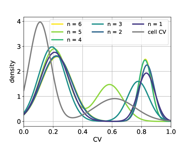
Figure 1: Bimodal fits of the histogram as a function of various different CVs that were computed from a set of trajectories from reference Gigli et al. (2022). here are multiple transitions between the tetragonal and cubic configurations in these trajectories. The two peaks in these distributions thus correspond to these two structures.

All $c_{nlm}^{i,a}$ coefficients, and the local polarizations $\mathbf{p}_{i}^{n}$ thereof, depend on the radial channel $n$. To determine which of the coefficients for the oxygen components is best at distinguishing the cubic and tetragonal phases we used all of them to analyse a series of trajectories in which multiple transitions between the tetragonal and cubic phases were observed. We also define a global, n-dependent, polarization for each BaTiO3 structure, as follows:

$$P_{n}=\sqrt{(C_{n1-1}^{O})^{2}+(C_{n10}^{O})^{2}+(C_{n1+1}^{O})^{2}}$$ (5)

where:

$$C_{nlm}^{a}=\sum_{i}c_{nlm}^{i,a}$$

and the sum runs over all central Ti atoms.

To generate figure 1 we constructed histograms for the trajectories as a function of $P_{n}$. As each histogram is bimodal a pair of Gaussians was then used to fit each of them. This analysis was performed for all 6 possible $n$ values as well as the following symmetrized combination of the cell parameters that we used in our previous work Gigli et al. (2022):

$$q=\frac{\sqrt{(a^{2}+b^{2}+c^{2})/3-(a+b+c)^{2}/9}}{\sqrt{a^{2}+b^{2}+c^{2}}}.$$ (6)

Four parameters must be determined when fitting the bimodal distribution: $\mu_{T}$ and $\mu_{C}$ are the centers of peaks that correspond to the cubic and tetragonal phases, while $\sigma_{T}$ and $\sigma_{C}$ are the corresponding standard deviations. Table 3 shows signal-to-noise ratios that calculated from these parameters for each of the CV choices shown in figure 1. By this measure, $q$ only outperforms the CV that is computed from the $C_{n1m}^{O}$ coefficients when $n=2$. This new set of CVs is thus better at distinguishing between the tetragonal and cubic phases.

References

- Bartók et al. (2010) Albert P. Bartók, Mike C. Payne, Risi Kondor, and Gábor Csányi, “Gaussian Approximation Potentials: The Accuracy of Quantum Mechanics, without the Electrons,” Phys. Rev. Lett. 104, 136403 (2010).
- Deringer et al. (2021) Volker L. Deringer, Albert P. Bartók, Noam Bernstein, David M. Wilkins, Michele Ceriotti, and Gábor Csányi, “Gaussian Process Regression for Materials and Molecules,” Chemical Reviews 121, 10073–10141 (2021), publisher: American Chemical Society.
- Musil et al. (2021) Félix Musil, Max Veit, Alexander Goscinski, Guillaume Fraux, Michael J. Willatt, Markus Stricker, Till Junge, and Michele Ceriotti, “Efficient implementation of atom-density representations,” The Journal of Chemical Physics 154, 114109 (2021).
- Goscinski et al. (2023) A Goscinski, VP Principe, G Fraux, S Kliavinek, BA Helfrecht, P Loche, M Ceriotti, and RK Cersonsky, “scikit-matter : A suite of generalisable machine learning methods born out of chemistry and materials science [version 2; peer review: 1 approved, 1 approved with reservations],” Open Research Europe 3 (2023), 10.12688/openreseurope.15789.2.
- Kresse and Furthmüller (1996) G Kresse and J Furthmüller, “Efficient iterative schemes for ab initio total-energy calculations using a plane-wave basis set,” Phys. Rev. B 54, 11169–11186 (1996).
- Giannozzi et al. (2009) Paolo Giannozzi, Stefano Baroni, Nicola Bonini, Matteo Calandra, Roberto Car, Carlo Cavazzoni, Davide Ceresoli, Guido L. Chiarotti, Matteo Cococcioni, Ismaila Dabo, Andrea Dal Corso, Stefano de Gironcoli, Stefano Fabris, Guido Fratesi, Ralph Gebauer, Uwe Gerstmann, Christos Gougoussis, Anton Kokalj, Michele Lazzeri, Layla Martin-Samos, Nicola Marzari, Francesco Mauri, Riccardo Mazzarello, Stefano Paolini, Alfredo Pasquarello, Lorenzo Paulatto, Carlo Sbraccia, Sandro Scandolo, Gabriele Sclauzero, Ari P. Seitsonen, Alexander Smogunov, Paolo Umari, and Renata M. Wentzcovitch, “QUANTUM ESPRESSO: a modular and open-source software project for quantum simulations of materials,” Journal of Physics: Condensed Matter 21, 395502 (2009).
- Gigli et al. (2022) Lorenzo Gigli, Max Veit, Michele Kotiuga, Giovanni Pizzi, Nicola Marzari, and Michele Ceriotti, “Thermodynamics and dielectric response of BaTiO3 by data-driven modeling,” npj Computational Materials 8, 1–17 (2022), number: 1 Publisher: Nature Publishing Group.