Bulk-edge correspondence for nonlinear eigenvalue problems

Abstract

Although topological phenomena attract growing interest not only in linear systems but also in nonlinear systems, the bulk-edge correspondence under the nonlinearity of eigenvalues has not been established so far. We address this issue by introducing auxiliary eigenvalues. We reveal that the topological edge states of auxiliary eigenstates are topologically inherited as physical edge states when the nonlinearity is weak but finite (i.e., auxiliary eigenvalues are monotonic as for the physical one). This result leads to the bulk-edge correspondence with the nonlinearity of eigenvalues.

Introduction.—The topological phase of matter has attracted considerable interest due to its exotic nature. In particular, topological band theory has played a crucial role in unveiling various types of topological phases by combining the principles of band theory and topology C.L.Kane_E.J.Mele_PRL.2005 ; C.L.Kane_E.J.Mele_PRL.2005_Z2 ; L.Fu_C.L.Kane_PRL.2007 ; M.Z.Hasan_C.L.Kane_RevModPhys.2010 ; X.L.Qi_S.C.Zhang_RevModPhys.2011 ; Y.Ando_JPSJ_2013 ; B.A.Bernevevig_T.L.Huglhes_S.C.Zhang_Science_2006 ; M.Knig_Science_2007 ; L.Fu_C.L.Kane_PRB.2007 ; L.Fu_C.L.Kane_PRB.2006 ; D.J.Thouless_PRB.1983 ; Schnyder_PRB.2008 ; A.Y.Kitaev_AIP_Conf_2009 ; S.Ryu_A.P.Schnyder_A.Furusaki_New.J.Phys_2010 ; X.L.Qi_T.L.Hughes_S.C.Zhang_PRB_2008 ; A.M.Essen_J.E.Moore_D.Vanderbilt_PRL_2009 ; S.Murakami_IOP_2007 ; W.Xiang_PRB_2011 ; Yang_PRB_2011 ; A.Birkov_PRL_2011 ; Xu_PRL_2011 ; Kurebayashi_JPSJ_2014 ; N.Armitage_RevModPhys_2018 ; Koshino_PRB_2016 . One of the most intriguing phenomena of topological phases is the bulk-edge correspondence (BEC), which indicates the edge states induced by the bulk-topology Hatsugai_BEC_PRL(1993) ; Hatsugai_BEC_PRB(1993) . Such topological edge states emerge regardless of other details of systems and are sources of anomalous behaviors. For instance, the robust edge states in integer quantum Hall systems result in quantized Hall conductance with extreme accuracy Klitzing_IQHE_PRL(1980) ; Laughlin_IQHE_PRB(1981) ; TKNN_IQHE_PRL(1982) ; Kohmoto_IQHE_AoP(1985) ; Haldane_AIQHE_PRL(1988) . Notably, in these years, the notion of topological states and BEC has expanded to encompass a broad range of systems, Raghu_PhC_PRL(2008) ; Raghu_PhC_PRA(2008) ; MIT_PhChIns_PRL(2008) ; Lu_TopPhot_Nat(2014) ; Hu_TopPhot_PRL(2015) ; Takahashi_Optica(2017) ; Takahashi_JPSJ(2018) ; Ozawa_TopPhot_RMP19 ; OtaIwamoto_NatPhoto(2020) ; Moritake_NanoPh(2021) ; Kariyado_MechGraph_Nat(2015) ; Yang_TopAco_PRL(2015) ; Huber_TopMech_Nat(2016) ; Susstrunk_MechClass_PNAS(2016) ; Tomoda_AIP(2017) ; Kawaguchi_Nature(2017) ; Takahashi_Mech_PRB(2019) ; Liu_TopPhon_AFM(2020) ; Lee_TopCir_Nat(2018) ; Yoshida_Difus_Nat(2021) ; Makino_Difus_PRE(2022) ; Hu_ObsDifs_AM(2022) ; Knebel_GameTheor_PRL(2020) ; Yoshida_GameTheor_PRE(2021) . including interdisciplinary systems, such as meteorological systems Delplace_TopoMeteo_science(2017) .

Along with the above progress, generalizing topological band theory has also elucidated exotic phenomena. For instance, while topological band theory originally developed for systems with Hermitian eigenvalue problems, generalizing it to non-Hermitian systems has discovered the emergence of exceptional points Zhen_ERing_nature(2015) ; Kozii_nH_arXiv(2017) ; Shen_NHTopBand_PRL(2018) ; Yoshida_NHhevferm_PRB(2018) ; Zyuzin_NHWyle_PRB(2018) ; Takata_pSSH_PRL(2018) ; Budich_SPERs_PRB(2019) ; Yoshida_SPERs_PRB(2019) ; Yoshida_PTEP(2020) ; Yoshida_SPERsMech_PRB(2019) ; Okugawa_SPERs_PRB(2019) ; Zhou_SPERs_Optica(2019) ; Mandal_HighEP_PRL(2021) ; Delplace_EP3_PRL(2021) ; IYH_PRB(2021) ; IYH_Nanoph(2023) and skin effects T.E.Lee_PRA_2016 ; Shunyu_PRL(2018)_SkinEffect ; Flore_skin_PRL(2018) ; Yoshida_MSkinPRR20 ; Yokomizo_nbloch_PRL(2019) ; Borgina-Jan_PRL(2020) ; Okuma_skin_PRL(2020) ; CFang_skin_PRL(2020) which do not have Hermitian counterparts.

In this respect, generalizing the topological band theory to nonlinear systems also induces novel phenomena. Indeed, the interplay between topology and nonlinearity of the eigenvectors has recently been discussed in Refs. Bloch_TopoSoliton_PRL(2019) ; Ezawa_NLTopo_PRB(2022) ; Ezawa_NLTopo_PRB(2022) ; Ezawa_NLTopo_JPSJ(2022) ; Sone_TopoSync_PRR(2022) ; Bloch_TopoSoliton_Nature(2022) ; Jezequel-Delplace_PRB_(2022) ; Sato-Fukui_TopoTodaLatt_JPSJ(2023) ; Sone_NLTopo_arxiv(2023) , elucidating topological synchronization induced by interplay between the nonlinearity and the topology Sone_TopoSync_PRR(2022) . Despite the above extensive efforts, the interplay between the topology and nonlinearity of eigenvalues, another type of nonlinearity, has not been discussed so far. In particular, BEC, which plays a central role, has not been established in nonlinear systems of eigenvalues. The significance of this issue is further enhanced by the existence of relevant systems; some of photonic crystals and mechanical metamaterials are described by the nonlinear eigenvalue problem Kuzmiak_Metal-PhC_PRB(1994) ; Huang_Mass-in-Mass_IJES(2009) .

In this letter, we establish the BEC for nonlinear systems of eigenvalues. Our strategy is based on an auxiliary eigenvalue. Introducing the auxiliary eigenvalue allows us to analyze the auxiliary edge states induced by the bulk-topology. Among them, focusing on the physical edge states leads us to the BEC under the nonlinearity of eigenvalues. We demonstrate the emergence of edge states due to nonlinear BEC for two-dimensional insulators and three-dimensional semimetals. Our approach of the auxiliary eigenvalue is considered to be versatile; it can be extended to systems in other symmetry classes and dimensions.

Figure 1: Schematic picture of the auxiliary bands $\lambda(k,\omega)$ for two-dimensional cylindrical system. The system is periodic in $y$-direction and with boundaries for $x$-direction. Bulk states are illustrated in green, while edge states are represented in red for each omega. The eigenstates that cross the $\lambda=0$ plane are of particular interest in the context of physics. Physical bands of $\omega(k)$ for each $k$ is shown in the inset. The gapless edge states of the auxiliary bands $\lambda$ are inherited to the physical nonlinear bands of $\omega$. Namely, red, blue, green, and white dots on the gray plane of $\lambda=0$ respectively corresponds to the physical edge states. For example, they can be dots in the inset.

Auxiliary eigenvalue and nonlinear bulk-edge correspondence.—Here, we provides our strategy to discuss the nonlinear BEC, i.e., the BEC of the nonlinear eigenvalue problems [see Eq. (1)]. We introduce the auxiliary eigenvalues and discuss the BEC between the bulk topology of the auxiliary bands and the physical edge states.

We consider the following nonlinear equation.

$$H(\omega,\bm{k})\psi=\omega S(\omega,\bm{k})\psi,$$ (1)

which is a nonlinear eigenvalue problem footnoteSone . Here, $H$ ($S$) is the Hamiltonian (overlap) matrix, $\psi$ is the eigenvector, and $\bm{k}$ is the wave number vector. We allow the matrices $H$ and $S$ may depend on the eigenvalue $\omega$ footnote1 ; footnote2 .

Now, we discuss BEC of nonlinear eigenvalue problems. As a first step, we consider the matrix pencil $P(\omega,\bm{k})$ Ikramov_MatPencil(1993) ,

$$P(\omega,\bm{k})=H(\omega,\bm{k})-\omega S(\omega,\bm{k}),$$ (2)

where the solution of $P(\omega,\bm{k})\psi=0$ is equivalent to Eq. (1). In order to discuss the BEC of Eq. (1), we introduce the auxiliary eigenvalue $\lambda$ and analyze its eigenvalue problems footnote3 ; footnoteLambda ,

$$P(\omega,\bm{k})\psi=\lambda\psi.$$ (3)

Here, $\lambda$ is auxiliary and does not have physical meaning except $\lambda=0$. The physical eigenvalue $\omega$ is a free parameter.

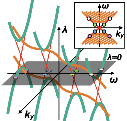
Next, we analyze Eq. (3) and discuss the BEC in the auxiliary bands of $\lambda$. Here, we need to assume $\lambda=0$ exists in the band gap of auxiliary eigenvalues. We note that the eigenstates only on $\lambda=0$ emerge in physics because auxiliary eigenvectors with finite $\lambda$ do not satisfy Eq. (1). When the bulk bands of $\lambda$ are topological, they possess gapless edge states under the open boundary condition. Since the edge states are gapless, those edge states cross $\lambda=0$ inevitably (see Fig. 1). Therefore, those edge states can be expected to emerge in physics.

Here, a comment is in order about the range of validity of the above discussion. The above discussion is valid when nonlinearity is weak in the vicinity of $\omega$ of interest (i.e., auxiliary eigenvalues are monotonic with respect to $\omega$). This is because the band indices of the bands of $\lambda$ and the bands of $\omega$ correspond one-to-one when the nonlinearity is weak. In this case, the gapless (gapped) nature of edge states of $\lambda$ is inherited to the bands of $\omega$. In contrast, when the nonlinearity is strong, band indices of the bands of $\lambda$ and the bands of $\omega$ do not correspond in general. In this case, the edge states of $\omega$ can be gapless even if the edge states of $\lambda$ are gapped. Thus, these gapless edge states cannot be characterized by the topological number, which is calculated by the eigenstates of $\lambda$ (for details, see Sec. I of Supplemental Material supple1 ). In addition, Eq. (1) can possess complex eigenvalues even when the matrices $H$ and $S$ are Hermitian under the strong nonlinearity. While the above cases are intriguing, strong nonlinearity induces additional complexities, which requires different approaches. Therefore, in the following discussion, we focus on the case where the nonlinearity is weak, i.e., the band indices of the bands of $\lambda$ and the bands of $\omega$ correspond, and $\lambda$ is real.

Figure 2: Band structure of the auxiliary eigenvalue $\lambda$ of the two-dimensional model. Edge (bulk) states are plotted in red (gray). (a1)-(c1) [(a2)-(c2)]: Plot of $\lambda$ for each $\omega$ [$k_{x}$] with $M_{0}=-1$, $M_{0}=0.35$, and $M_{0}=1$ respectively. The parameter $k_{x}$ ($\omega$) is fixed in $k_{x}=0$ ($\omega=1$). Parameter $k_{x}$ ($\omega$) is choosen in $k_{x}=0$ ($\omega$=1). Edge states emerge when $M_{0}<0.35$.

Figure 3: Band structure of $\omega$ of the two-dimensional model. Edge (bulk) states are plotted in red (gray). (a)-(c): Plot of $\omega$ for each $k_{x}$ and the Chern number of the bands of $\lambda$ with $M_{0}=-1$, $M_{0}=0.35$, and $M_{0}=1$ respectively. The band gap is fully opening in the orange-colored regions. (d): Plot of the Chern number calculated from the eigenstates of $\lambda_{1}$ for each $M_{0}$ and $\omega$. The Chern number takes a non-zero (zero) value in the blue-colored region. The black line represents $\omega=1$. The band structures in Figs. 3(a), 3(b), and 3(c) emerge on the black, red, and green dots. The region where the Chern number takes non-zero values corresponds to the region where the edge states emerge.

Nonlinear Chern insulator and gapless edge states.—Here, we explore the nonlinear BEC in a two-dimensional model. We examine the relationship between the bulk topology of the auxiliary bands of $\lambda$ and the gapless edge states of $\omega$ in a two-dimensional system described by a nonlinear eigenvalue problem [Eq. (1)].

Here, we analyze the following two-dimensional model with $\omega$-dependent terms,

$$H(\bm{k})=\begin{pmatrix}E+M_{\mathrm{H}}(\bm{k})&\mathrm{sin}(k_{x})-i\mathrm{sin}(k_{y})\\ \mathrm{sin}(k_{x})+i\mathrm{sin}(k_{y})&E-M_{\mathrm{H}}(\bm{k})\end{pmatrix},$$ (4)

$$S(\omega)=\begin{pmatrix}1-M_{\mathrm{S}}(\omega)&0\\ 0&1+M_{\mathrm{S}}(\omega)\end{pmatrix},$$ (5)

with $E=1$, $M_{\mathrm{H}}(\bm{k})=M_{0}+\sum_{i=x,y}[1-\mathrm{cos}(k_{i})]$, and $M_{\mathrm{S}}(\omega)=M_{1}\mathrm{tanh}(\omega)/\omega$. Here, $M_{1}$ is fixed to $0.5$. We denote this system by a nonlinear Chern insulator (for the case of the chiral symmetric system, see Sec. II of Supplemental Material [60]). From these matrices, matrix $P$ is given by,

$$P(\omega,\bm{k})=\begin{pmatrix}E_{\mathrm{P}}(\omega)+M_{\mathrm{P}}(\omega,\bm{k})&\mathrm{sin}(k_{x})-i\mathrm{sin}(k_{y})\\ \mathrm{sin}(k_{x})+i\mathrm{sin}(k_{y})&E_{\mathrm{P}}(\omega)-M_{\mathrm{P}}(\omega,\bm{k})\end{pmatrix},$$ (6)

with $E_{\mathrm{P}}(\omega)=E-\omega$ and $M_{\mathrm{P}}(\omega,\bm{k})=M_{\mathrm{H}}(\bm{k})+\omega M_{\mathrm{S}}(\omega)$.

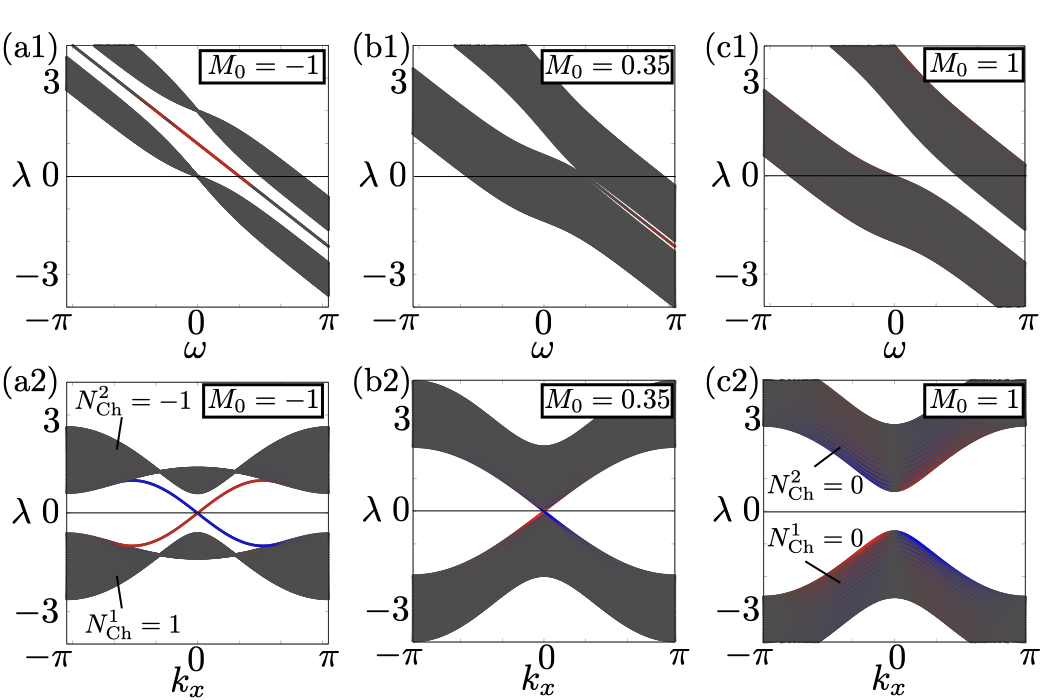
Here, let us analyze the auxiliary band structure of $\lambda$ by solving the eigenvalue problem $P(\omega,\bm{k})\psi=\lambda\psi$. The band structure of $\lambda$ is plotted in Fig. 2. For the calculations of Fig. 2, we consider the open (periodic) boundary conditions in the $y$-direction ($x$-direction). Figures 2(a1)-2(c1) [2(a2)-2(c2)] displays auxiliary eigenvalues $\lambda$ for each $\omega$ ($k_{x}$) with $k_{x}=0$ ($\omega=1$). Bulk (edge) states are plotted in gray (red). When $M_{0}=-1$, edge states emerge [see Figs.  2(a1) and 2(a2)]. Since these edge states are gapless in the momentum space, the edge states cross $\lambda=0$ inevitably. This result suggests the existence of physical edge states inherited from the auxiliary bands. In Figs. 2(b1) and 2(b2), the band gap closes at $M_{0}=0.35$. The point of $\lambda(\omega=1,k_{x}=0)$ becomes the Dirac point. When $M_{0}=1$, the band gap reopens, and the edge states vanish. From these results, we can conclude that the topological phase transition occurs at $M_{0}=0.35$. Therefore, when $M_{0}<0.35$, we can expect the presence of physical edge states since the edge states of auxiliary bands cross $\lambda=0$ inevitably.

In order to characterize the gapless edge states in Fig. 2, let us consider the topological number of the auxiliary bands of $\lambda$. For our two-dimensional model, the Chern number can be used as a topological number. The Chern number of the band index $n$ is defined by,

$$N_{\mathrm{Ch}}^{n}(\omega)=\frac{1}{2\pi}\int_{1BZ}dk_{x}dk_{y}\bm{\nabla}_{k}\times\bm{A}_{n}(\omega,\bm{k}),$$ (7)

$$\bm{A}_{n}(\omega,\bm{k})=\langle\psi_{n,k}(\omega)|\bm{\nabla}_{k}\psi_{n,k}(\omega)\rangle,$$ (8)

where $|\psi_{n,\bm{k}}(\omega)\rangle$ is an auxiliary eigenstate with band index $n$ and momentum $\bm{k}$. The integration is conducted in the first Brillouin zone of the momentum space. In our model, Berry connection $\bm{A}_{n}(\omega,\bm{k})$ depend on $\omega$. Thus, the Chern number becomes the function of $\omega$.

In our model, the Chern number takes non-zero values when $M_{0}<0.35$. In Fig. 2(a2), the Chern number of the lower (upper) band is $N_{\mathrm{Ch}}^{1}(\omega_{\mathrm{R}})=1$ [$N_{\mathrm{Ch}}^{2}(\omega_{\mathrm{R}})=-1$] while $N_{\mathrm{Ch}}^{1}(\omega_{\mathrm{R}})=N_{\mathrm{Ch}}^{2}(\omega_{\mathrm{R}})=0$ in Fig. 2(c2) with $\omega_{\mathrm{R}}=\omega=1$. Therefore, the Chern number calculated by the eigenstates of $\lambda$ corresponds to the number of edge states of the auxiliary bands of $\lambda$.

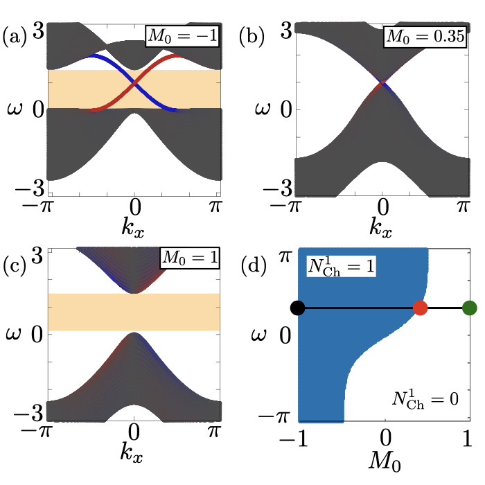
Here, let us investigate the nonlinear BEC between the above Chern number and the edge states of $\omega$. The physical band structures of $\omega$ are plotted in Fig. 3 by extracting the data of $\lambda=0$. In Figs. 3(a)-3(c), the bands of $\omega$ are plotted for each $k_{x}$ with $M_{0}=-1$, $M_{0}=0.35$, and $M_{0}=1$ respectively. Bulk (edge) states are plotted in gray (red or blue). For the calculation of these figures, the open (periodic) boundary condition is imposed in the $y$- ($x$-) direction. The region where the band gap of $\omega$ remains open across all $k_{x}$ is colored with orange. In our model, the gapless edge states of $\omega$ emerge when $M_{0}=-1$ [see Fig. 3(a)]. The edge states are inherited from the edge states of $\lambda$ plotted in Fig. 2(a2). The band structure of $\omega$ become gapless when $M_{0}=0.35$ [see Fig. 3(b)]. This gapless point corresponds to the gap-closing point in Fig. 2(b2), which elucidates a nonlinear topological phase transition. When $M_{0}=1$, the edge states vanish [see Fig. 3(c)].

Figure 3(d) is the plot of the Chern number of the lower band obtained from the eigenstates of $\lambda$ for each $M_{0}$ and $\omega$. The Chern number takes a non-zero value in the blue-colored region. The black line represents $\omega=1$. The band structures plotted Figs. 3(a), 3(b), and 3(c) emerge on the black, red, and green dots in Fig. 3(d). Importantly, correspondence exists between the regions where the Chern number is non-zero and the regions where edge states emerge. The above results demonstrate that the nonlinear BEC holds for nonlinear Chern insulator.

Here, we note that when discussing the nonlinear BEC from the phase diagram plotted in Fig. 3(d), $\omega_{\mathrm{R}}$ is properly chosen so that it is inside of the band gap of $\omega$. Taking $\omega_{R}$ outside the band gap can lead to a mismatch between the Chern number and the edge states.

Figure 4: Plot of the Chern number calculated by the eigenstates of $\lambda$ for each $k_{z}$ and $\omega$. The Chern number takes 1 (0) in the blue (white) region. The black line represents $\omega=1$. Band structures of Figs. 3(a), 3(b), and 3(c) emerge on the black, red, and green dots. The boundaries between the blue and the white regions correspond to the Weyl nodes.

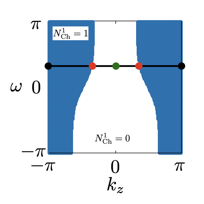
Nonlinear topological semimetal and Fermi arc surface states.—Next, let us consider the nonlinear BEC in a three-dimensional model. We demonstrate the existence of the nonlinear BEC between the bulk topology of the auxiliary bands and the Fermi-arc surface states of the nonlinear Weyl semimetals (see below) by analyzing a three-dimensional model including $\omega$-dependent term.

Here, we analyze Eqs. (4)-(6) with $M_{0}=\mathrm{cos}(k_{z})$. In this model, the gapless band structure plotted in Fig. 3(b) emerges at $\mathrm{cos}(k_{z})=-0.35$. These gapless points of $\omega$ correspond to the Weyl points, which form a line structure in the four-dimensional parameter space, composed of $\omega$, $k_{x}$, $k_{y}$ and $k_{z}$. The band structure in Fig. 3(a) [(b)] also emerges at $k_{z}=\pi$ [$k_{z}=0$]. In this manner, we define a system described by the nonlinear eigenvalue problems that possess pairs of Weyl points as nonlinear Weyl semimetals.

Figure 4 is the plot of the Chern number of the lower band obtained from the eigenstates of $\lambda$ for each $k_{z}$ and $\omega$. The blue (white) region represents where the Chern number takes $1$ ($0$). The black line represents $\omega=1$, and colored dots indicate the points where the band structures plotted in Fig. 3 emerge. On the black, red, and green points, The band structure plotted in Fig. 3(a), 3(b), and 3(c) emerges. In Fig. 4, the boundaries between the blue and white colored region correspond to the Weyl nodes. In our model, Weyl nodes form line structures in the $k_{z}$-$\omega$ space. However, in general, these lines of Weyl points emerge in the four-dimensional parameter space composed of $k_{x}$, $k_{y}$, $k_{z}$, and $\omega$. Notably, as is the case of the two-dimensional model, the correspondence exists between the region where the Chern number takes a non-zero value and the region where edge states emerge. This result shows the applicability of nonlinear BEC even in the topological semimetals.

Summary.— In this letter, we have established the BEC for nonlinear systems of eigenvalues. We have introduced an auxiliary eigenvalue and showed the emergence of BEC between the bulk topology of auxiliary eigenstates and physical edge states when the nonlinearity is weak. Applying our argument to two-dimensional insulators and three-dimensional semimetals, we have demonstrated the emergence of edge states induced by the nonlinear BEC. Our results show BEC remains valid even beyond the linear systems. Our nonlinear BEC is applicable to the model with more complicated $\omega$-dependence as long as the nonlinearity is weak (i.e., auxiliary eigenvalues are monotonic with respect to $\omega$). Our approach with the auxiliary eigenvalue is considered to be extended to systems in other symmetry classes and dimensions. These extensions and applications to more physical setups are left as future works.

Acknowledgement.—This work is supported by MEXT-JSPS Grant-in-Aid for Transformative Research Areas (A) “Extreme Universe”: Grant No. JP22H05247. This work is also supported by JST-CREST Grant No. JPMJCR19T1, JST-SPRING Grant No. JPMJSP2124, and JSPS KAKENHI Grant No. JP21K13850, JP23H01091. TY is grateful to the long term workshop YITP-T-23-01 held at YITP, Kyoto University.

References

- (1) C. L. Kane and E. J. Mele, Phys. Rev. Lett. 95, 226801 (2005).
- (2) C. L. Kane and E. J. Mele, Phys. Rev. Lett. 95, 146802 (2005).
- (3) L. Fu, C. L. Kane, and E. J. Mele, Phys. Rev. Lett. 98, 106803 (2007).
- (4) M. Z. Hasan and C. L. Kane, Rev. Mod. Phys. 82, 3045 (2010).
- (5) X.-L. Qi and S.-C. Zhang, Rev. Mod. Phys. 83, 1057 (2011).
- (6) Y. Ando, Journal of the Physical Society of Japan 82, 102001 (2013).
- (7) B. A. Bernevig, T. L. Hughes, and S.-C. Zhang, science 314, 1757 (2006).
- (8) M. König, S. Wiedmann, C. Brüne, A. Roth, H. Buhmann, L. W. Molenkamp, X.-L. Qi, and S.-C. Zhang, Science 318, 766 (2007).
- (9) L. Fu and C. L. Kane, Phys. Rev. B 76, 045302 (2007).
- (10) L. Fu and C. L. Kane, Phys. Rev. B 74, 195312 (2006).
- (11) D. J. Thouless, Phys. Rev. B 27, 6083 (1983).
- (12) A. P. Schnyder, S. Ryu, A. Furusaki, and A. W. W. Ludwig, Phys. Rev. B 78, 195125 (2008).
- (13) A. Kitaev, Periodic table for topological insulators and superconductors, in AIP conference proceedings Vol. 1134, pp. 22–30, American Institute of Physics, 2009.
- (14) S. Ryu, A. P. Schnyder, A. Furusaki, and A. W. Ludwig, New Journal of Physics 12, 065010 (2010).
- (15) X.-L. Qi, T. L. Hughes, and S.-C. Zhang, Phys. Rev. B 81, 159901 (2010).
- (16) A. M. Essin, J. E. Moore, and D. Vanderbilt, Phys. Rev. Lett. 102, 146805 (2009).
- (17) S. Murakami, New Journal of Physics 9, 356 (2007).
- (18) X. Wan, A. M. Turner, A. Vishwanath, and S. Y. Savrasov, Phys. Rev. B 83, 205101 (2011).
- (19) K.-Y. Yang, Y.-M. Lu, and Y. Ran, Phys. Rev. B 84, 075129 (2011).
- (20) A. A. Burkov and L. Balents, Phys. Rev. Lett. 107, 127205 (2011).
- (21) G. Xu, H. Weng, Z. Wang, X. Dai, and Z. Fang, Phys. Rev. Lett. 107, 186806 (2011).
- (22) D. Kurebayashi and K. Nomura, Journal of the Physical Society of Japan 83, 063709 (2014).
- (23) N. P. Armitage, E. J. Mele, and A. Vishwanath, Rev. Mod. Phys. 90, 015001 (2018).
- (24) M. Koshino and I. F. Hizbullah, Phys. Rev. B 93, 045201 (2016).
- (25) Y. Hatsugai, Phys. Rev. Lett. 71, 3697 (1993).
- (26) Y. Hatsugai, Phys. Rev. B 48, 11851 (1993).
- (27) K. v. Klitzing, G. Dorda, and M. Pepper, Phys. Rev. Lett. 45, 494 (1980).
- (28) R. B. Laughlin, Phys. Rev. B 23, 5632 (1981).
- (29) D. J. Thouless, M. Kohmoto, M. P. Nightingale, and M. den Nijs, Phys. Rev. Lett. 49, 405 (1982).
- (30) M. Kohmoto, Annals of Physics 160, 343 (1985).
- (31) F. D. M. Haldane, Phys. Rev. Lett. 61, 2015 (1988).
- (32) F. D. M. Haldane and S. Raghu, Phys. Rev. Lett. 100, 013904 (2008).
- (33) S. Raghu and F. D. M. Haldane, Phys. Rev. A 78, 033834 (2008).
- (34) Z. Wang, Y. D. Chong, J. D. Joannopoulos, and M. Soljačić, Phys. Rev. Lett. 100, 013905 (2008).
- (35) L. Lu, J. D. Joannopoulos, and M. Soljačić, Nature photonics 8, 821 (2014).
- (36) L.-H. Wu and X. Hu, Phys. Rev. Lett. 114, 223901 (2015).
- (37) S. Takahashi, S. Oono, S. Iwamoto, Y. Hatsugai, and Y. Arakawa, Optical weyl points below the light line in semiconductor chiral woodpile photonic crystals, in Conference on Lasers and Electro-Optics, p. JTu5A.42, Optica Publishing Group, 2017.
- (38) S. Takahashi, S. Oono, S. Iwamoto, Y. Hatsugai, and Y. Arakawa, Journal of the Physical Society of Japan 87, 123401 (2018).
- (39) T. Ozawa, H. M. Price, A. Amo, N. Goldman, M. Hafezi, L. Lu, M. C. Rechtsman, D. Schuster, J. Simon, O. Zilberberg, and I. Carusotto, Rev. Mod. Phys. 91, 015006 (2019).
- (40) Y. Ota, K. Takata, T. Ozawa, A. Amo, Z. Jia, B. Kante, M. Notomi, Y. Arakawa, and S. Iwamoto, Nanophotonics 9, 547 (2020).
- (41) Y. Moritake, M. Ono, and M. Notomi, Nanophotonics 11, 2183 (2022).
- (42) T. Kariyado and Y. Hatsugai, Scientific reports 5, 1 (2015).
- (43) Z. Yang, F. Gao, X. Shi, X. Lin, Z. Gao, Y. Chong, and B. Zhang, Phys. Rev. Lett. 114, 114301 (2015).
- (44) S. D. Huber, Nature Physics 12, 621 (2016).
- (45) R. Süsstrunk and S. D. Huber, Proceedings of the National Academy of Sciences 113, E4767 (2016).
- (46) S. Mezil, K. Fujita, P. H. Otsuka, M. Tomoda, M. Clark, O. B. Wright, and O. Matsuda, Applied Physics Letters 111, 144103 (2017).
- (47) K. Kawaguchi, R. Kageyama, and M. Sano, Nature 545, 327 (2017).
- (48) Y. Takahashi, T. Kariyado, and Y. Hatsugai, Phys. Rev. B 99, 024102 (2019).
- (49) Y. Liu, X. Chen, and Y. Xu, Advanced Functional Materials 30, 1904784.
- (50) C. H. Lee, S. Imhof, C. Berger, F. Bayer, J. Brehm, L. W. Molenkamp, T. Kiessling, and R. Thomale, Communications Physics 1, 1 (2018).
- (51) T. Yoshida and Y. Hatsugai, Scientific reports 11, 1 (2021).
- (52) S. Makino, T. Fukui, T. Yoshida, and Y. Hatsugai, Phys. Rev. E 105, 024137 (2022).
- (53) H. Hu, S. Han, Y. Yang, D. Liu, H. Xue, G.-G. Liu, Z. Cheng, Q. J. Wang, S. Zhang, B. Zhang, and Y. Luo, Advanced Materials n/a, 2202257.
- (54) J. Knebel, P. M. Geiger, and E. Frey, Phys. Rev. Lett. 125, 258301 (2020).
- (55) T. Yoshida, T. Mizoguchi, and Y. Hatsugai, Phys. Rev. E 104, 025003 (2021).
- (56) P. Delplace, J. B. Marston, and A. Venaille, Science 358, 1075 (2017).
- (57) B. Zhen, C. W. Hsu, Y. Igarashi, L. Lu, I. Kaminer, A. Pick, S.-L. Chua, J. D. Joannopoulos, and M. Soljačić, Nature 525, 354 (2015).
- (58) V. Kozii and L. Fu, arXiv preprint arXiv:1708.05841 (2017).
- (59) H. Shen, B. Zhen, and L. Fu, Phys. Rev. Lett. 120, 146402 (2018).
- (60) T. Yoshida, R. Peters, and N. Kawakami, Phys. Rev. B 98, 035141 (2018).
- (61) A. A. Zyuzin and A. Y. Zyuzin, Phys. Rev. B 97, 041203 (2018).
- (62) K. Takata and M. Notomi, Phys. Rev. Lett. 121, 213902 (2018).
- (63) J. C. Budich, J. Carlström, F. K. Kunst, and E. J. Bergholtz, Phys. Rev. B 99, 041406 (2019).
- (64) T. Yoshida, R. Peters, N. Kawakami, and Y. Hatsugai, Phys. Rev. B 99, 121101 (2019).
- (65) T. Yoshida, R. Peters, N. Kawakami, and Y. Hatsugai, Progress of Theoretical and Experimental Physics 2020 (2020), 12A109.
- (66) T. Yoshida and Y. Hatsugai, Phys. Rev. B 100, 054109 (2019).
- (67) R. Okugawa and T. Yokoyama, Phys. Rev. B 99, 041202 (2019).
- (68) H. Zhou, J. Y. Lee, S. Liu, and B. Zhen, Optica 6, 190 (2019).
- (69) I. Mandal and E. J. Bergholtz, Phys. Rev. Lett. 127, 186601 (2021).
- (70) P. Delplace, T. Yoshida, and Y. Hatsugai, Phys. Rev. Lett. 127, 186602 (2021).
- (71) T. Isobe, T. Yoshida, and Y. Hatsugai, Phys. Rev. B 104, L121105 (2021).
- (72) T. Isobe, T. Yoshida, and Y. Hatsugai, Nanophotonics 12, 2335 (2023).
- (73) T. E. Lee, Phys. Rev. Lett. 116, 133903 (2016).
- (74) S. Yao and Z. Wang, Phys. Rev. Lett. 121, 086803 (2018).
- (75) F. K. Kunst, E. Edvardsson, J. C. Budich, and E. J. Bergholtz, Phys. Rev. Lett. 121, 026808 (2018).
- (76) T. Yoshida, T. Mizoguchi, and Y. Hatsugai, Phys. Rev. Research 2, 022062 (2020).
- (77) K. Yokomizo and S. Murakami, Phys. Rev. Lett. 123, 066404 (2019).
- (78) D. S. Borgnia, A. J. Kruchkov, and R.-J. Slager, Phys. Rev. Lett. 124, 056802 (2020).
- (79) N. Okuma, K. Kawabata, K. Shiozaki, and M. Sato, Phys. Rev. Lett. 124, 086801 (2020).
- (80) K. Zhang, Z. Yang, and C. Fang, Phys. Rev. Lett. 125, 126402 (2020).
- (81) V. Goblot, B. Rauer, F. Vicentini, A. Le Boité, E. Galopin, A. Lemaître, L. Le Gratiet, A. Harouri, I. Sagnes, S. Ravets, C. Ciuti, A. Amo, and J. Bloch, Phys. Rev. Lett. 123, 113901 (2019).
- (82) M. Ezawa, Phys. Rev. B 106, 195423 (2022).
- (83) M. Ezawa, Journal of the Physical Society of Japan 91, 024703 (2022).
- (84) K. Sone, Y. Ashida, and T. Sagawa, Phys. Rev. Res. 4, 023211 (2022).
- (85) N. Pernet et al., Nature Physics 18, 678 (2022).
- (86) L. Jezequel and P. Delplace, Phys. Rev. B 105, 035410 (2022).
- (87) K. Sato and T. Fukui, Journal of the Physical Society of Japan 92, 073001 (2023).
- (88) K. Sone, M. Ezawa, Y. Ashida, N. Yoshioka, and T. Sagawa, Nonlinearity-induced topological phase transition characterized by the nonlinear chern number, 2023, arXiv:2307.16827.
- (89) V. Kuzmiak, A. A. Maradudin, and F. Pincemin, Phys. Rev. B 50, 16835 (1994).
- (90) H. Huang, C. Sun, and G. Huang, International Journal of Engineering Science 47, 610 (2009).
- (91) In Ref. Sone_TopoSync_PRR(2022) , the word “nonlinear eigenvalue problem” is employed to describe the nonlinearity of eigenvectors which differs from the terminology in this paper.
- (92) If and are independent from , Eq. (1) is reduced to generalized eigenvalue problem. If is independent from and is the identity matrix, Eq. (1) is reduced to the ordinary eigenvalue problem.
- (93) We note that some of photonic crystals are described by the nonlinear eigenvalue problem. In these systems, the frequency dependence of permittivity (permeability) results in dependence of matrix () Kuzmiak_Metal-PhC_PRB(1994) .
- (94) K. D. Ikramov, Journal of Soviet Mathematics 64, 783 (1993).
- (95) The auxiliary eigenvalues of the matrix pencil are analyzed in Ref. Raghu_PhC_PRA(2008) in the context of the stability of eigenvalues. In this letter, we employ it to establish the BEC of the nonlinear eigenvalue problem.
- (96) We note that how to introduce is not uniquely determined. For example, it is possible to introduce a matrix so that Eq. (3) becomes a generalized eigenvalue problem .
- (97) Supplemental material for the discussion of monotonicity of auxiliary eigenvalue .