Julearn: an easy-to-use library for leakage-free evaluation and inspection of ML models

Abstract

Background

The fast-paced development of machine learning (ML) methods coupled with its increasing adoption in research poses challenges for researchers without extensive training in ML. In neuroscience, for example, ML can help understand brain-behavior relationships, diagnose diseases, and develop biomarkers using various data sources like magnetic resonance imaging and electroencephalography. The primary objective of ML is to build models that can make accurate predictions on unseen data. Researchers aim to prove the existence of such generalizable models by evaluating performance using techniques such as cross-validation (CV), which uses systematic subsampling to estimate the generalization performance. Choosing a CV scheme and evaluating an ML pipeline can be challenging and, if used improperly, can lead to overestimated results and incorrect interpretations.

Findings

We created julearn, an open-source Python library, that allow researchers to design and evaluate complex ML pipelines without encountering in common pitfalls. In this manuscript, we present the rationale behind julearn’s design, its core features, and showcase three examples of previously-published research projects that can be easily implemented using this novel library.

Conclusions

Julearn aims to simplify the entry into the ML world by providing an easy-to-use environment with built in guards against some of the most common ML pitfalls. With its design, unique features and simple interface, it poses as a useful Python-based library for research projects.

Keywords Machine Learning  $\cdot$ Research Software Library  $\cdot$ Neuroscience

1 Introduction

ML is fast becoming an indispensable tool in many research fields. It is rapidly gaining increasing importance within neuroscience, where it is used for understanding brain-behavior relationships Wu et al. (2023), predicting disease status and biomarker development using diverse data modalities such as MRI and EEG. Such thriving applications of ML are driven by availability of big data and advances in computing technologies. Yet, for domain experts, acquiring relevant ML and programming skills remains a significant challenge. This underscores the need for user-friendly software solutions accessible to domain experts without extensive ML training. Such solutions would enable them to quickly evaluate ML approaches.

The goal of an ML application is to create a model that provides accurate predictions on new unseen data—i.e., a generalizable model. In this context, the goal of a research project is usually to demonstrate that a generalizable model exists for the prediction task at hand. As a single set of samples is usually available, this goal is achieved by assessing the generalization performance by training the model on a subset of the data and testing it on the hold-out test data. If the model performs well on the test data, then the researcher concludes that the prediction task can be solved in a generalizable manner. One of the most prominent approaches to estimate the generalization performance is CV. CV is a systematic subsampling approach, which trains and tests ML pipelines multiple times using independent data splits Varoquaux et al. (2017). The average performance over the splits is taken as an estimate of generalization. To achieve good performance or other aims like data interpretation it is often necessary to perform additional data processing, for example, feature selection. This results in an ML pipeline that performs all the needed operations from data manipulations, training and evaluation. Choosing a CV scheme and evaluating an ML pipeline can be challenging, and if improperly used, it can lead to incorrect results and misguided insights. This underscores the need for user-friendly software solutions accessible to domain experts without in-depth ML and programming training. Problematically, a common outcome of pitfalls is an overestimation of the generalization performance when using CV, i.e. models are reported as being more accurate than what they actually are. Here, we highlight two common pitfalls; data leakage and overfitting of hyperparameters.

Data leakage occurs when the separation between the training and test data is not strictly followed. For instance, using all available data in parts of an ML pipeline breaks the required separation between training and test data. Such data leakage invalidates the complete CV procedure, as information of the testing set is available during training. For example, one might apply a preprocessing step like z-standardization, or PCA on the complete dataset before splitting the data. As the preprocessing step is informed about the test data, the later created and transformed training data will reflect the test data as well. Therefore, the learning algorithm can leverage this leaked test set information through the preprocessing and memorize instead of building a predictive model, thus inflating the generalization estimation of CV. Most problematically, data leakage can happen in many ways through programming errors or lacking awareness of this danger.

A similar pitfall can occur when tuning hyperparameters by first observing their test set performance. Hyperparameters are parameters, not learnable by the algorithms themselves, which greatly impact their prediction performance. To tackle this optimization problem, many practitioners repeat a simple CV to evaluate test set performance of different hyperparameter combinations. Problematically, both tuning and estimating out-of-sample performance on the same test data breaks the clear distinction of training and testing, as one both optimizes and evaluates the ML pipeline on the same test set. Notably, this can happen very quickly over the natural progression of research projects while iterating through ideas of appropriate hyperparameters. The solution to this pitfall is to select the hyperparameters and evaluate the out-of-sample performance in different data splits, which can be achieved by using a nested CV. In conclusion, both pitfalls can happen very easily without any malicious intent, through a lack of ML or programming experience. We developed the open-source python package julearn to allow field experts to circumvent these pitfalls by default while training and evaluating ML pipelines.

While ML experts can navigate these and other pitfalls using expert software, such as scikit-learn, domain experts might not always be aware of the pitfalls or how to handle them. This is why we created julearn, to provide an out-of-the box solution, preventing common mistakes, usable by domain experts. Julearn was created to be easy to use, to be accessible for researchers with diverse backgrounds, and to create reproducible results. Furthermore, we engineered julearn so it is easy to extend and maintain, in order to keep up with constantly evolving fields such as neuroscience and medicine. The accessibility and usability aspects of julearn were decided to be at the core, as we aimed to help researchers to apply ML. We accomplished this through a careful design of the API, comprising only a few simple key functions and classes to both create and evaluate complex ML pipelines. Furthermore, we added several utilities that allow investigators to gain a detailed understanding of the resulting pipelines. In order to keep julearn up to date, we built it on top of scikit-learn Pedregosa et al. (2012); Abraham et al. (2014) and followed common best practices of software engineering like unit testing and continuous integration.

2 Methods

2.1 Basic Usage

Julearn is built on top of scikit-learn Pedregosa et al. (2012); Abraham et al. (2014), one of the most influential ML libraries in the Python programming language. While scikit-learn provides a powerful interface for programmers to create complex and individualized ML pipelines, julearn mainly adds an abstraction layer, providing a simple interface for novice programmers. Note that in contrast to scikit-learn, julearn focusses on so called supervised ML tasks, which include any prediction task with known labels while training and evaluating pipelines. Therefore, pipelines in the context of julearn always refer to supervised ML pipelines.

To achieve a simple interface for supervised ML problems, we implemented a core function called run_cross_validation to estimate a models’ performance using CV. In this function, the user specifies the data, features, target, preprocessing and model name to evaluate as a ML pipeline in a leakage-free cross-validated manner. We chose the popular and simple tabular data structure of pandas’ DataFrame McKinney (2010) for both the input data and the output of run_cross_validation. This makes preparing the input, inspecting and analyzing the output of julearn simple and transparent.

Furthermore, our API provides arguments for feature and target name(s) referring to the columns of the input data frame. To use any of julearn’s ML algorithms one only needs to provide their name to the model argument of run_cross_validation. Here, julearn will select the model according to the provided problem_type of either classification or regression. Similarly, one can provide any of the supported preprocessing steps to run_cross_validation by name. These steps are executed in a CV-consistent way without the risk of data leakage. Such an interface simplifies the construction and use of ML pipelines, in contrast to scikit-learn, where one must import different ML models depending on the problem type, create a pipeline using both the imported preprocessing steps and the ML model and finally use the cross_validate function (Figure 1).

While julearn does not aim to replace scikit-learn, it tries to simplify specific use cases including the creation of more complex supervised ML pipelines that need hyperparameter tuning or preprocessing a subsample of features. This means that julearn can automatically use nested CV for proper performance assessment in the context of hyperparameter tuning Poldrack et al. (2020) and apply preprocessing based on different feature types. These feature types include distinctions like categorical vs continuous features or grouping variables, which can even be used to do confound removal on a subsample of the data.

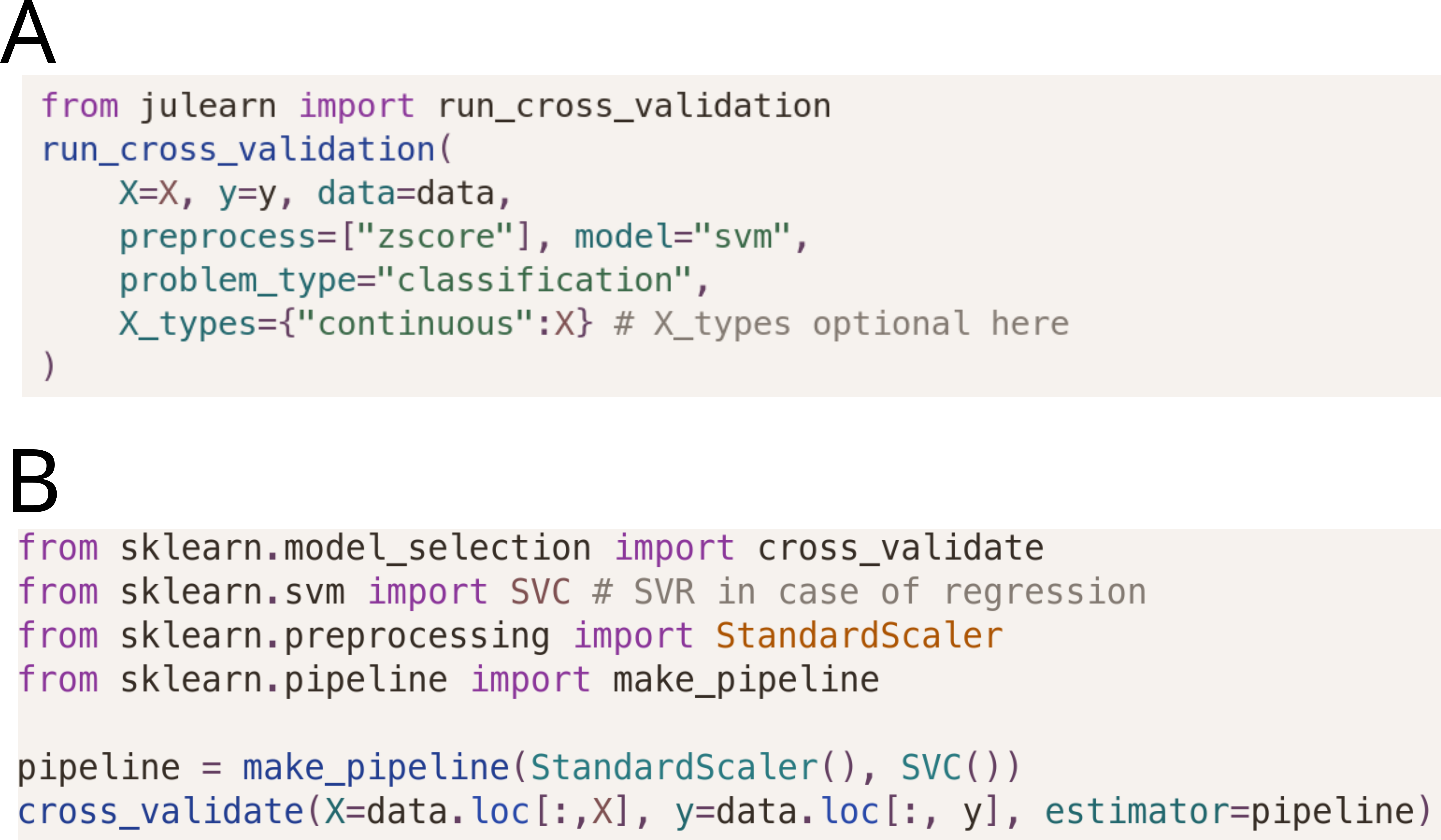
Figure 1: Implementation of a simple CV pipeline using julearn (A) in contrast to scikit-learn (B). The julearn pipeline needs only one import, while scikit-learn needs multiple. Furthermore, scikit-learn needs to import the Support Vector Machine differently depending on the problem type, while julearn chooses the correct one based on the problem type. The differences between julearn and scikit-learn is most influential for non-experienced programmers who aim to create (complex) supervised ML pipelines. Julearn builds upon scikit-learn by providing a simple interface that does not need any awareness of how to compose and find different classes.

2.2 Model Comparison

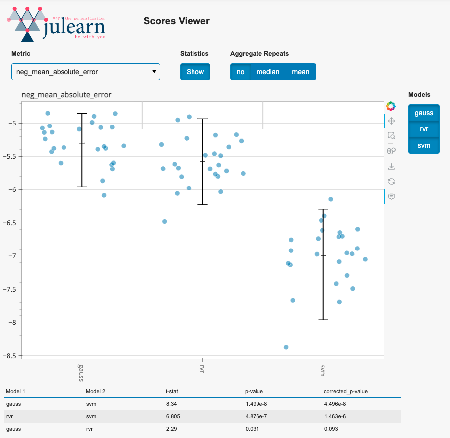
Figure 3: Screenshot of the julearn scores viewer, depicting the negative mean absolute error in age prediction from gray matter volume. Each dot represents the negative mean absolute error of each CV fold (5 times, 5-folds). Each column represents a different model: GPR (gauss), RVR (rvr) and SVR (svm). Black lines indicate the mean and 95% confidence intervals. Table at the bottom shows the pairwise statistics using the corrected t-test.

In ML applications, there is no standard or consensus of what a good or acceptable performance is, as this usually depends on the task and domain. Thus, the process of developing predictive models involves comparing models, either to null or dummy models, or to previously published models (i.e. benchmarking). Given that CV produces estimates of the model’s performance and that, depending on the CV strategy, these estimates might not be independent from each other, special methods are required to test and conclude if the performance of two models are different or not. For this reason, julearn run_cross_validation output has additional information that can be used to do more accurate model comparisons. Furthermore, it provides a stats module, which implements a student’s t-test corrected for using the same CV approach to compare multiple ML pipelines Nadeau and Bengio (2003). This correction is necessary as CV leads to a dependencency between the folds, i.e., each iteration’s training set overlaps with the other ones. To gain a detailed view of the models’ benchmark, one can also use julearn’s inbuilt visualization tool (see Figure 3 for example).

2.3 Feature Types

One of the key functionalities that julearn provides that are currently lacking in ML libraries such as scikit-learn is the ability to define feature types. This allows researchers to define sets of variables and do selective processing, needed when dealing with categorical or confounding variables. For this matter, julearn introduces the PipelineCreator to create complex pipelines in which certain processing steps can be applied to one or more subset of features. Once the pipeline is defined, users need to provide a dictionary of any user-defined type and the associated column names in their data as the X_types argument. Such functionality allows to implement complex pipelines that transform features based on their type, e.g., standardizing only continuous features and then deconfound both continuous and categorical features.

2.4 Hyperparameter Tuning

As mentioned previously, hyperparameter tuning should be performed in a nested CV to not overfit the predictions of a given pipeline. The PipelineCreator can be used to specify sets of hyperparameters to be tested at each individual step by just using the add method (Figure 2). Being able to first define a pipeline and its hyperparameters with the PipelineCreator, and to then train and evaluate this pipeline with run_cross_validation, makes performing leakage-free nested CV easy. In this nested CV, all hyperparameters are optimized in an inner CV using a grid search by default. This default, like most of julearn’s defaults, can be easily adjusted by providing any compatible searcher in the run_cross_validation’s model_params argument. This is a drastic simplification compared to a typical scikit-learn workflow, where one must create the pipeline manually by combining different objects, wrap it inside a GridSearchCV object, and define the hyperparameter options separately from the pipeline itself, using a complex syntax. Lastly, scikit-learn’s GridSearchCV object must be provided to its cross_validate function.

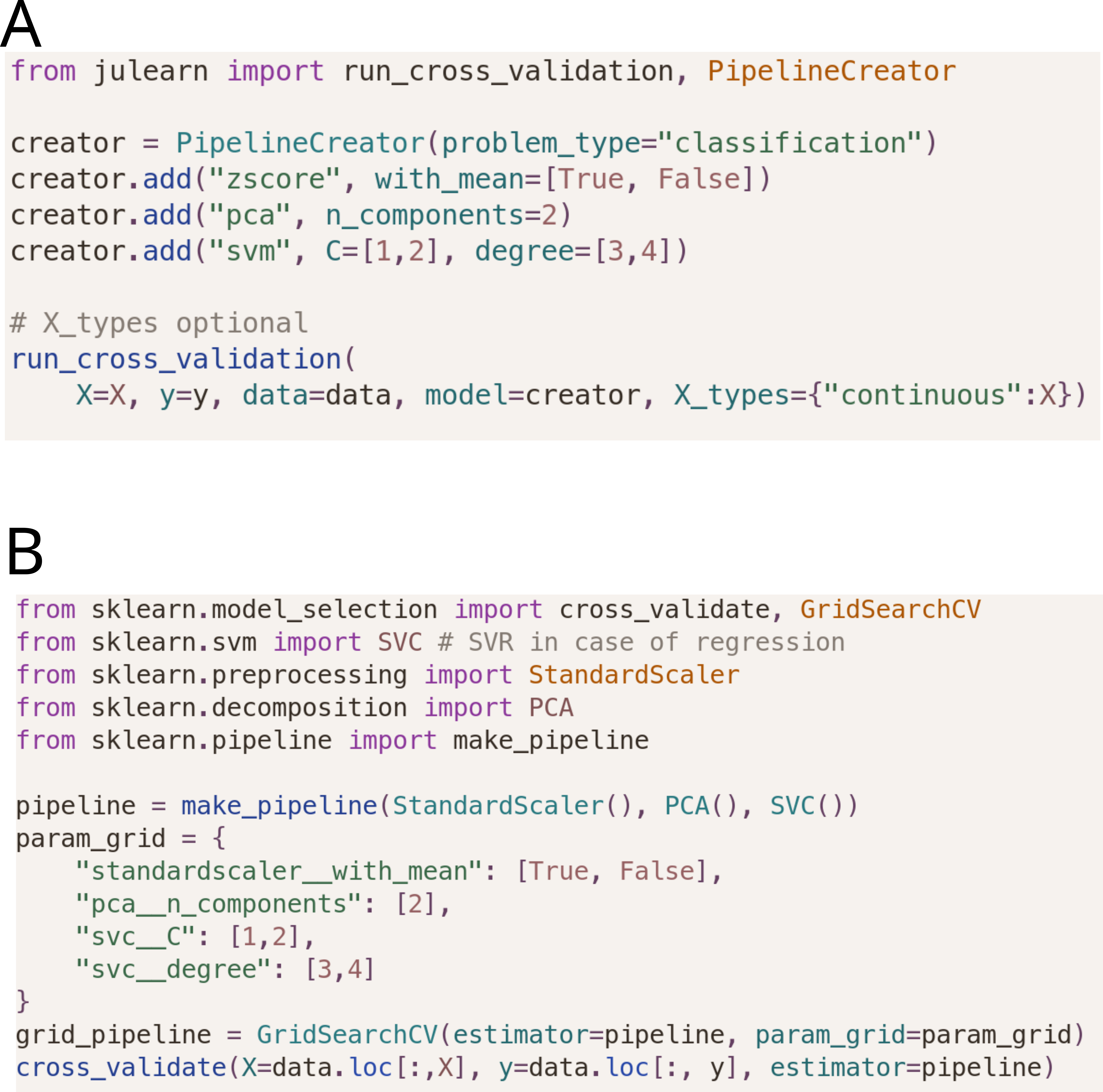
Figure 2: Example of julearn (A) and scikit-learn (B) training a typical ML pipeline in a CV consistent way. Both use a grid search to find optimal hyperparameters. Note that julearn is able to specify the hyperparameters at the same time as it defines each step. On the other hand, scikit-learn needs all hyperparameters to be defined separately with a prefix indicating the step they belong to. This can become complex especially when pipelines are nested, and multiple prefixes are needed.

2.5 Inspection and Analysis

Inspection of ML pipelines is crucial when working in fields such as neuroscience and medicine as concepts like trustworthy ML are heavily dependent on the ability to draw insights and conclusions from models. For this purpose, one needs to be able to inspect and verify each of the pipeline steps, check parameters, evaluate feature importances and further properties of ML pipelines. Julearn includes two functionalities: a preprocess_until function and Inspector class. The preprocess_until function allows users to process the data up to any step of the pipeline, allowing to check how the different transformations are applied. For example, a user might be interested in examining the PCA components created or the distribution of features after confound removal. The Inspector object, on the other hand, allows us to inspect the models after estimating their performance using CV. It helps users to check fold-wise predictions and obtain both the hyper- and fitted parameters of the trained models. This enables users to verify the robustness of the different parameter combinations and evaluate the variability of the performance across folds. Ongoing efforts to increase julearn’s inspection tools encompass integrating tools for explainable AI such as SHAP Lundberg and Lee .

2.6 Neuroscience-specific Features

In addition to julearn’s field-agnostic features, we also provide neuroscience-specific functionality. Confound removal in the form of confound regression, which is popularly used in neuroscience, was implemented as the ConfoundRemover. This confound regression can be trained on all features or only on specific subsamples defined by a grouping variable, i.e., allowing neuroscientist to only train it on healthy participants as proposed in Dukart et al. (2011). Additionally, we have included the CBPM algorithm Shen et al. (2017). This transformer aggregates features significantly correlated with the target into one or two features. This can be done separately for the positively and negatively correlated features. Aggregation can be done using any user specified aggregation function such as summation or mean. We plan to add more neuroscience specific features, such as the integration of harmonization techniques, currently developed in a separate project (juharmonize).

2.7 Customization and Extensibility

Julearn provides a simple interface to several important ML approaches, but it is also easily customizable. Each component of julearn is built to be scikit-learn compatible, meaning that any scikit-learn compatible model and transformer can be provided to run_cross_validation and PipelineCreator. Other run_cross_validation arguments like cv and hyperparameter searchers were implemented in a way to be extensible by any typical scikit-learn object. This customizability of julearn helps users both extend their usage of julearn and prepares them for the case that they want to transition to scikit-learn to build unique expert level ML pipelines.

3 Examples

To illustrate the functionality and quality attributes of julearn, we depict three independent examples, showing how the analysis described in previously-published research projects can be implemented with julearn.

3.1 Example 1: Prediction of age using GMV derived from T1-weighted MRI images.

Dataset

We used T1-weighted (T1w) MRI images from the publicly available IXI dataset (https://brain-development.org/ixi-dataset/) (IXI, N = 562, age range = 20-86 years) for age estimation similar to Franke et al. (2010).

Image Preprocessing

T1w images were preprocessed using the CAT version 12.8 Gaser and Dahnke . Initial affine registration of T1w images was done with higher than default accuracy (accstr = 0.8), to ensure accurate normalization and segmentation. After bias field correction and tissue class segmentation, accurate optimized Geodesic shooting Ashburner and Friston (2011) was used for normalization (regstr = 1). We used 1 mm Geodesic Shooting templates and generated 1 mm isotropic images as output. Next, the normalized GM segments were modulated for linear and non-linear transformations.

Feature spaces and models

A whole-brain mask was used to select 238,955 GM voxels. Then, smoothing with a 4mm FWHM Gaussian kernel and resampling using linear interpolation to 8 mm spatial resolution was applied resulting in 3747 features. We tested three regression models GPR, RVR and SVR using this feature space to predict age.

Prediction Analysis

We used 5 times 5-fold CV to estimate generalization performance of our pipelines. Hyperparameters were tuned in the inner 5-fold CV. Features with low variance were removed (threshold < 1e-5). PCA was applied on the features to retain 100% variance. GPR model gave lowest generalization error (mean MAE = -5.30 years), followed by RVR (MAE = -5.56) and SVR (MAE = -6.98). Corrected t-test revealed significant difference between GPR and SVM (p = 3.18e-09) and RVR and SVM (p = 8.19e-09). There was no significant difference between RVR and GPR (p = 0.075).

3.2 Example 2: Confound Removal.

Dataset

For this example, we retrieved data conceptually similar to Dukart et al. (2011). We used the ADNI database including 498 participants and 68 features. We used age as a confound and the current diagnosis as the target. To simplify the task, we only predict whether a participant has some form of impairment (mild cognitive impairment or Alzheimer’s disease) or not (control).

Prediction Analysis

We aimed to conceptually replicate figure 1 from Dukart et al. (2011). The authors proposed to train confound regression on the healthy participants of a study and then transform all participants using this confound regression. As part of their efforts, they compared two pipelines using the same learning algorithm (SVM) Berwick and Idiot (1990). One pipeline was trained to directly classify healthy vs unhealthy participants without controlling for age, while a second pipeline was configured to first control for age using their proposed method: train the confound regression only on healthy participants. They evaluated the bias of age in the predictions of these models by comparing the age distributions of the healthy vs unhealthy participants for each model’s misclassifications. This was done by computing, for each pipeline, whether there is a significant age difference between these two groups of participants. They found a significant difference when not controlling for age, but not when controlling for age. With further experiments, they conclude that their method leads to less age-related bias. In this example, we replicate the comparison between the two SVMs. First, we built both pipelines using julearn and then compared their misclassified predictions to find the same differences (Figure 4).

While the first pipeline (without confound removal) is straightforward to implement, the second variant requires a complicated preprocessing step in which the confound removal needs to be trained on a subsample of one specific column of the data. Thanks to julearn’s support for feature types, the whole procedure can be easily implemented by indicating which feature type are to be considered confounds (e.g.: age), which column has the subsampling data (e.g.: current diagnosis) and which values should be considered (e.g.: healthy). Note that the difference between all subjects in age also gets significant for our larger, but not their smaller, sample, which can be attributed to the increased power due to the large sample size.

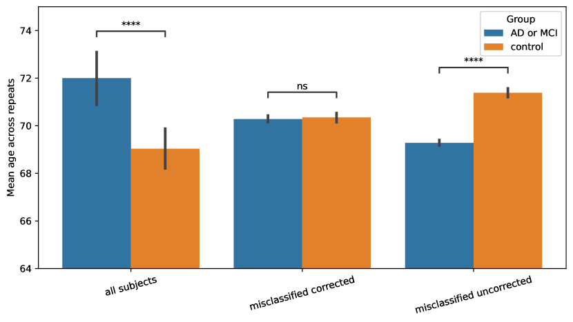
Figure 4: Replication of figure 1 in “Age characteristics of misclassified subjects using SVM” from Dukart et al. (2011). Performing a cross-validated confound removal trained only on the control group using julearn. Julearn greatly simplifies the process to train CV consistent preprocessing steps based on characteristics like control vs experimental group. **** means a statistical significance at a p-value threshold of 0.0001 and ns that there is no statistical difference at that threshold.

3.3 Example 3: Prediction of fluid intelligence using Connectome-Based Predictive Modelling.

Dataset

We used data obtained from two rs-fMRI sessions from the HCP-YA S1200 release Van Essen et al. (2013). The details regarding collection of behavioral data, rs-fMRI acquisition, and image preprocessing have been described elsewhere Glasser et al. (2013); Barch et al. (2013). Here, we provide a an overview. The scanning protocol for HCP-YA was approved by the local Institutional Review Board at Washington University in St. Louis. Retrospective analysis of these datasets was further approved by the local Ethics Committee at the Faculty of Medicine at Heinrich-Heine-University in Düsseldorf. We selected sessions for both phase encoding directions (left-to-right [LR] and right-to-left [RL]) obtained on the first day of HCP-YA data collection. Due to the HCP-YA’s family structure, we selected 399 unrelated subjects (matched for the variable “Gender”), so that we could always maintain independence between folds during cross-validation. In line with Finn et al. (2015), we filtered out subjects with high estimates of overall head motion (frame-to-frame head motion estimate (averaged across both day 1 rest runs; HCP-YA: Movement_RelativeRMS_mean > 0.14). This resulted in a dataset consisting of 368 subjects (176 female, 192 male). Participants’ ages ranged from 22 to 37 (M=28.7, SD=3.85). The two sessions of rs-fMRI each lasted 15 minutes, resulting in 30 minutes across both sessions. Scans were acquired using a 3T Siemens connectome-Skyra scanner with a gradient-echo EPI sequence (TE=33.1ms, TR=720ms, flip angle = 52°, 2.0mm isotropic voxels, 72 slices, multiband factor of 8).

Image Preprocessing

Data from rs-fMRI sessions in the HCP-YA had already undergone the HCP’s minimal preprocessing pipeline Glasser et al. (2013)(, including motion correction and registration to standard space. Additionally, the ICA-FIX procedure Salimi-Khorshidi et al. (2014) was applied to remove structured artefacts. Lastly, the 6 rigid-body parameters, their temporal derivatives and the squares of the 12 previous terms were regressed out, resulting in 24 parameters. In addition, we regressed out mean time courses of the WM, CSF, and GS, as well as their squared terms, and the temporal derivatives of the mean signals as well as their squared terms as confounds, resulting in 12 parameters (4 for each noise component). The signal was linearly detrended and bandpass filtered at 0.01 - 0.08 Hz using nilearn.image.clean_img, The resulting voxel-wise time series were then aggregated using the Shen parcellation Finn et al. (2015) consisting of 268 parcels. FC was estimated for each rs-fMRI session as Pearson’s correlation between each pair of parcels, resulting in a symmetric 268x268 matrix. These two FC matrices were further averaged resulting in one FC matrix per subject. One half of the symmetric matrix as well as the diagonal were discarded so that only unique edges were used as features in the prediction workflow.

Prediction Analysis

First, we aimed to reproduce Finn et al. (2015) prediction pipeline using the CBPM framework using the LOO-CV scheme. Specifically, we reconstructed the workflow used to reproduce Fig 5a in Finn et al. (2015). As a prediction target we used subjects’ score on the Penn Matrix Test (PMAT24_A_CR. This is a non-verbal reasoning assessment and a measure of fluid intelligence. CBPM first performs correlation-based univariate feature selection based on a pre-specified significance threshold. Selected features are further divided into positively and negatively correlated features, and then separately summed up, resulting in two features. Subsequently, a linear regression is fitted either on both or one of these features based on user preference. The results here were obtained by using the positive-feature network at a feature selection threshold of p < .01 in line with Fig. 5a from Finn et al. (2015). We observe a similar trend in our results albeit with a lower correlation between observed and predicted values (see Figure 5). In addition, we also provide results for a 10-Fold cross-validation with 10 repeats. In this analysis, we also tested CBPM using positive- and negative-feature networks individually as well as both feature networks combined with varying thresholds for feature selection (0.01, 0.05, 0.1).

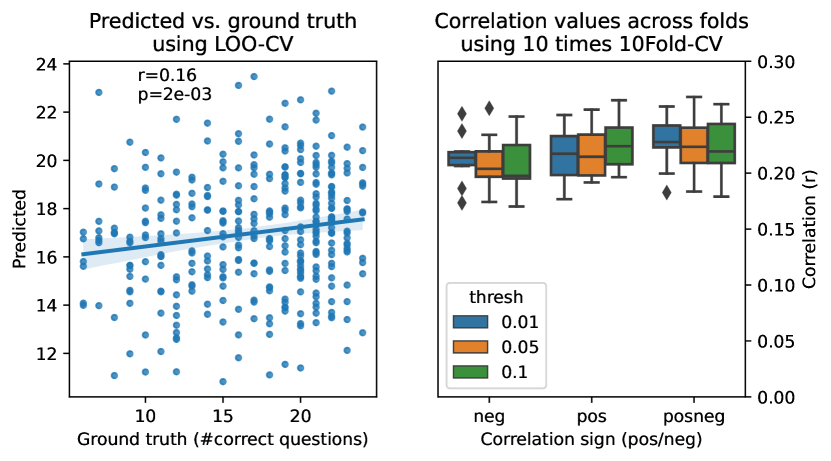
Figure 5: results of the prediction of fluid intelligence using CBPM on HCP-YA data as in Finn et al. (2015). Left panel depicts the predicted (y-axis) vs the ground truth (x-axis) values for each sample in a LOO-CV scheme, following figure 5a in Finn et al. (2015). Right panel depicts the mean correlation values (r) across folds, for a 10-times 10-fold CV scheme, using different thresholds (colors) and considering either negative correlations, positive correlations, or both kinds of correlations (columns).

4 Discussion

Julearn aims to bridge the gap between domain expertise in neuroscience and application of ML pipelines. Towards that goal, julearn provides a simple interface only using two key API points. First, the run_cross_validation function provides functionality to evaluate common ML pipelines. Second the PipelineCreator provides means to devise complex ML pipelines that can be then evaluated using run_cross_validation. Additional functionalities are also provided to guide and help users to inspect and evaluate the resulting CV scores. In fact, julearn provides a complete workflow for ML that has already been used in several publications Mortaheb et al. (2022); More et al. (2023). Furthermore, the customizability and open-source nature of julearn will help it grow and extend its functionality in the future.

Julearn does not aim to replace core ML libraries such as scikit-learn. Rather its aim is to simplify the entry into the ML world by providing an easy-to-use environment with built in guards against some of the most common ML pitfalls, such as data leakage that can happen due to not using nested cross-validation and when performing confound removal. Furthermore, julearn is not created to compete with AutoML approaches Ferreira et al. (2021); Zöller and Huber (2021); Waring et al. (2020) which try to automate the preprocessing and modelling over multiple algorithms and sets of hyperparameters. While these approaches are valid and powerful, they yet do not offer full functionality such as nested cross validation and confound removal required in many bio-medical research fields. Furthermore, a researcher might require more control over type of models, parameters and interpretability which might not be easily achievable with current AutoML libraries. Lastly, there are other libraries such as photonLeenings et al. (2021), Neurominer noa (a) or Neuropredict noa (b) that try to build on top of powerful ML libraires to create different interfaces with unique features for field experts. All these libraries are important for a vibrant open-source community, and julearn‘s unique features and simple interface will be useful for many research projects.

5 Availability of source code

Julearn’s code is available in GitHub https://github.com/juaml/julearn with the corresponding documentation in GitHub Pages https://juaml.github.io/julearn/. The code used for the examples in this manuscript is available at https://github.com/juaml/julearn_paper, with instructions on how to get the publicly available data.

• Project name: Julearn

• Project home page: https://juaml.github.io/julearn/

• Operating system(s): Platform independent

• Programming language: Python

• License: GNU AGPLv3

6 Data availability

The data use in this manuscript is publicly available following each dataset requirements. Information on the dataset sources is provided in the description of each example.

7 Declarations

7.1 List of abbreviations

7.2 Consent for publication

Consent for publication was obtained from the Alzheimer’s Disease Neuroimaging Initiative (ADNI; https://adni.loni.usc.edu/) Data and Publications Committee. Other datasets do not require consent for publication.

7.3 Competing Interests

The author(s) declare that they have no competing interests’.

7.4 Funding

This work was partly supported by the Helmholtz-AI project DeGen (ZT-I-PF-5-078), the Helmholtz Portfolio Theme “Supercomputing and Modeling for the Human Brain” the Deutsche Forschungsgemeinschaft (DFG, German Research Foundation), project PA 3634/1-1 and project-ID 431549029–SFB 1451 project B05, the Helmholtz Imaging Platform and eBRAIN Health (HORIZON-INFRA-2021-TECH-01).

Data collection and sharing for this project was funded by the Alzheimer’s Disease Neuroimaging Initiative (ADNI) (National Institutes of Health Grant U01 AG024904) and DOD ADNI (Department of Defense award number W81XWH-12-2-0012). ADNI is funded by the National Institute on Aging, the National Institute of Biomedical Imaging and Bioengineering, and through generous contributions from the following: AbbVie, Alzheimer’s Association; Alzheimer’s Drug Discovery Foundation; Araclon Biotech; BioClinica, Inc.; Biogen; Bristol-Myers Squibb Company; CereSpir, Inc.; Cogstate; Eisai Inc.; Elan Pharmaceuticals, Inc.; Eli Lilly and Company; EuroImmun; F. Hoffmann-La Roche Ltd and its affiliated company Genentech, Inc.; Fujirebio; GE Healthcare; IXICO Ltd.; Janssen Alzheimer Immunotherapy Research & Development, LLC.; Johnson & Johnson Pharmaceutical Research & Development LLC.; Lumosity; Lundbeck; Merck & Co., Inc.; Meso Scale Diagnostics, LLC.; NeuroRx Research; Neurotrack Technologies; Novartis Pharmaceuticals Corporation; Pfizer Inc.; Piramal Imaging; Servier; Takeda Pharmaceutical Company; and Transition Therapeutics. The Canadian Institutes of Health Research is providing funds to support ADNI clinical sites in Canada. Private sector contributions are facilitated by the Foundation for the National Institutes of Health (www.fnih.org). The grantee organization is the Northern California Institute for Research and Education, and the study is coordinated by the Alzheimer’s Therapeutic Research Institute at the University of Southern California. ADNI data are disseminated by the Laboratory for Neuro Imaging at the University of Southern California.

7.5 Author’s Contributions

S.H. and F.R. designed the library. S.H, L.S., V.K., S.M., K.R.P. and F.R.. contributed to the development and testing of the library, wrote and reviewed the manuscript. V.K. contributed to the structural design and writing of julearn’s documentation. S.M. and F.R. wrote the code for Example 1, S.H. and F.R. wrote the code for Example 2 and L.S. wrote the code for Example 3.

8 Acknowledgements

We want to thank the INM-7 and early adopters of julearn for their valuable contribution at early stages, shaping the direction of our efforts in developing this tool.

References

- Wu et al. [2023] Jianxiao Wu, Jingwei Li, Simon B. Eickhoff, Dustin Scheinost, and Sarah Genon. The challenges and prospects of brain-based prediction of behaviour. Nature Human Behaviour, 7(8):1255–1264, August 2023. ISSN 2397-3374. doi:10.1038/s41562-023-01670-1. URL https://www.nature.com/articles/s41562-023-01670-1. Number: 8 Publisher: Nature Publishing Group.
- Varoquaux et al. [2017] Gaël Varoquaux, Pradeep Reddy Raamana, Denis A. Engemann, Andrés Hoyos-Idrobo, Yannick Schwartz, and Bertrand Thirion. Assessing and tuning brain decoders: Cross-validation, caveats, and guidelines. NeuroImage, 145:166–179, January 2017. doi:10.1016/j.neuroimage.2016.10.038. URL http://linkinghub.elsevier.com/retrieve/pii/S105381191630595X.
- Pedregosa et al. [2012] Fabian Pedregosa, Gaël Varoquaux, Alexandre Gramfort, Vincent Michel, Bertrand Thirion, Olivier Grisel, Mathieu Blondel, Peter Prettenhofer, Ron Weiss, Vincent Dubourg, Jake Vanderplas, Alexandre Passos, David Cournapeau, Matthieu Brucher, Matthieu Perrot, and Édouard Duchesnay. Scikit-learn: Machine Learning in Python. Journal of Machine Learning Research, 12:2825–2830, 2012. ISSN 1532-4435. doi:10.1007/s13398-014-0173-7.2. URL http://dl.acm.org/citation.cfm?id=2078195%5Cnhttp://arxiv.org/abs/1201.0490.
- Abraham et al. [2014] Alexandre Abraham, Fabian Pedregosa, Michael Eickenberg, Philippe Gervais, Andreas Mueller, Jean Kossaifi, Alexandre Gramfort, Bertrand Thirion, and Gaël Varoquaux. Machine learning for neuroimaging with scikit-learn. Frontiers in Neuroinformatics, 8, 2014. ISSN 1662-5196. doi:10.3389/fninf.2014.00014. URL http://journal.frontiersin.org/article/10.3389/fninf.2014.00014/abstract. ZSCC: 0000341.
- McKinney [2010] Wes McKinney. Data Structures for Statistical Computing in Python. pages 56–61, Austin, Texas, 2010. doi:10.25080/Majora-92bf1922-00a. URL https://conference.scipy.org/proceedings/scipy2010/mckinney.html.
- Poldrack et al. [2020] Russell A. Poldrack, Grace Huckins, and Gael Varoquaux. Establishment of Best Practices for Evidence for Prediction: A Review. JAMA Psychiatry, 77(5):534–540, May 2020. ISSN 2168-622X. doi:10.1001/jamapsychiatry.2019.3671. URL https://doi.org/10.1001/jamapsychiatry.2019.3671.
- Nadeau and Bengio [2003] Claude Nadeau and Yoshua Bengio. Inference for the Generalization Error. Machine Learning, 52(3):239–281, September 2003. ISSN 1573-0565. doi:10.1023/A:1024068626366. URL https://doi.org/10.1023/A:1024068626366.
- [8] Scott M Lundberg and Su-In Lee. A Unified Approach to Interpreting Model Predictions.
- Dukart et al. [2011] Juergen Dukart, Matthias L. Schroeter, Karsten Mueller, and The Alzheimer’s Disease Neuroimaging Initiative. Age Correction in Dementia – Matching to a Healthy Brain. PLOS ONE, 6(7):e22193, July 2011. ISSN 1932-6203. doi:10.1371/journal.pone.0022193. URL https://journals.plos.org/plosone/article?id=10.1371/journal.pone.0022193. Publisher: Public Library of Science.
- Shen et al. [2017] Xilin Shen, Emily S. Finn, Dustin Scheinost, Monica D. Rosenberg, Marvin M. Chun, Xenophon Papademetris, and R Todd Constable. Using connectome-based predictive modeling to predict individual behavior from brain connectivity. Nature protocols, 12(3):506–518, March 2017. ISSN 1754-2189. doi:10.1038/nprot.2016.178. URL https://www.ncbi.nlm.nih.gov/pmc/articles/PMC5526681/.
- Franke et al. [2010] Katja Franke, Gabriel Ziegler, Stefan Klöppel, Christian Gaser, and Alzheimer’s Disease Neuroimaging Initiative. Estimating the age of healthy subjects from T1-weighted MRI scans using kernel methods: exploring the influence of various parameters. NeuroImage, 50(3):883–892, April 2010. ISSN 1095-9572. doi:10.1016/j.neuroimage.2010.01.005.
- [12] Christian Gaser and Robert Dahnke. CAT - A Computational Anatomy Toolbox for the Analysis of Structural MRI Data. page 1.
- Ashburner and Friston [2011] John Ashburner and Karl J. Friston. Diffeomorphic registration using geodesic shooting and Gauss–Newton optimisation. NeuroImage, 55(3):954–967, April 2011. ISSN 1053-8119. doi:10.1016/j.neuroimage.2010.12.049. URL https://www.sciencedirect.com/science/article/pii/S1053811910016496.
- Berwick and Idiot [1990] R Berwick and Village Idiot. An Idiot ’ s guide to Support vector machines ( SVMs ) SVMs : A New Generation of Learning Algorithms Key Ideas. pages 1–28, 1990.
- Van Essen et al. [2013] David C. Van Essen, Stephen M. Smith, Deanna M. Barch, Timothy E. J. Behrens, Essa Yacoub, Kamil Ugurbil, and WU-Minn HCP Consortium. The WU-Minn Human Connectome Project: an overview. NeuroImage, 80:62–79, October 2013. ISSN 1095-9572. doi:10.1016/j.neuroimage.2013.05.041.
- Glasser et al. [2013] Matthew F. Glasser, Stamatios N. Sotiropoulos, J. Anthony Wilson, Timothy S. Coalson, Bruce Fischl, Jesper L. Andersson, Junqian Xu, Saad Jbabdi, Matthew Webster, Jonathan R. Polimeni, David C. Van Essen, and Mark Jenkinson. The minimal preprocessing pipelines for the Human Connectome Project. NeuroImage, 80:105–124, October 2013. ISSN 10538119. doi:10.1016/j.neuroimage.2013.04.127. URL https://linkinghub.elsevier.com/retrieve/pii/S1053811913005053.
- Barch et al. [2013] Deanna M. Barch, Gregory C. Burgess, Michael P. Harms, Steven E. Petersen, Bradley L. Schlaggar, Maurizio Corbetta, Matthew F. Glasser, Sandra Curtiss, Sachin Dixit, Cindy Feldt, Dan Nolan, Edward Bryant, Tucker Hartley, Owen Footer, James M. Bjork, Russ Poldrack, Steve Smith, Heidi Johansen-Berg, Abraham Z. Snyder, David C. Van Essen, and WU-Minn HCP Consortium. Function in the human connectome: task-fMRI and individual differences in behavior. NeuroImage, 80:169–189, October 2013. ISSN 1095-9572. doi:10.1016/j.neuroimage.2013.05.033.
- Finn et al. [2015] Emily S. Finn, Xilin Shen, Dustin Scheinost, Monica D. Rosenberg, Jessica Huang, Marvin M. Chun, Xenophon Papademetris, and R. Todd Constable. Functional connectome fingerprinting: identifying individuals using patterns of brain connectivity. Nature Neuroscience, 18(11):1664–1671, November 2015. ISSN 1546-1726. doi:10.1038/nn.4135. URL https://www.nature.com/articles/nn.4135. Number: 11 Publisher: Nature Publishing Group.
- Salimi-Khorshidi et al. [2014] Gholamreza Salimi-Khorshidi, Gwenaëlle Douaud, Christian F. Beckmann, Matthew F. Glasser, Ludovica Griffanti, and Stephen M. Smith. Automatic denoising of functional MRI data: combining independent component analysis and hierarchical fusion of classifiers. NeuroImage, 90:449–468, April 2014. ISSN 1095-9572. doi:10.1016/j.neuroimage.2013.11.046.
- Mortaheb et al. [2022] Sepehr Mortaheb, Laurens Van Calster, Federico Raimondo, Manousos A. Klados, Paradeisios Alexandros Boulakis, Kleio Georgoula, Steve Majerus, Dimitri Van De Ville, and Athena Demertzi. Mind blanking is a distinct mental state linked to a recurrent brain profile of globally positive connectivity during ongoing mentation. Proceedings of the National Academy of Sciences, 119(41):e2200511119, October 2022. doi:10.1073/pnas.2200511119. URL https://www.pnas.org/doi/full/10.1073/pnas.2200511119. Publisher: Proceedings of the National Academy of Sciences.
- More et al. [2023] Shammi More, Georgios Antonopoulos, Felix Hoffstaedter, Julian Caspers, Simon B. Eickhoff, Kaustubh R. Patil, and Alzheimer’s Disease Neuroimaging Initiative. Brain-age prediction: A systematic comparison of machine learning workflows. NeuroImage, 270:119947, April 2023. ISSN 1095-9572. doi:10.1016/j.neuroimage.2023.119947.
- Ferreira et al. [2021] Luís Ferreira, André Pilastri, Carlos Manuel Martins, Pedro Miguel Pires, and Paulo Cortez. A Comparison of AutoML Tools for Machine Learning, Deep Learning and XGBoost. In 2021 International Joint Conference on Neural Networks (IJCNN), pages 1–8, July 2021. doi:10.1109/IJCNN52387.2021.9534091. URL https://ieeexplore.ieee.org/abstract/document/9534091?casa_token=dCG-spkGZPUAAAAA:8vtWBWFov7GfKvJJNx3uk61fx8TEfcwpi0J5Y5vw0fWLasgkWuYQUNcMlHs8HpjUfjQo19Fx2Aau. ISSN: 2161-4407.
- Zöller and Huber [2021] Marc-André Zöller and Marco F. Huber. Benchmark and Survey of Automated Machine Learning Frameworks. Journal of Artificial Intelligence Research, 70:409–472, January 2021. ISSN 1076-9757. doi:10.1613/jair.1.11854. URL https://www.jair.org/index.php/jair/article/view/11854.
- Waring et al. [2020] Jonathan Waring, Charlotta Lindvall, and Renato Umeton. Automated machine learning: Review of the state-of-the-art and opportunities for healthcare. Artificial Intelligence in Medicine, 104:101822, April 2020. ISSN 0933-3657. doi:10.1016/j.artmed.2020.101822. URL https://www.sciencedirect.com/science/article/pii/S0933365719310437.
- Leenings et al. [2021] Ramona Leenings, Nils Ralf Winter, Lucas Plagwitz, Vincent Holstein, Jan Ernsting, Kelvin Sarink, Lukas Fisch, Jakob Steenweg, Leon Kleine-Vennekate, Julian Gebker, Daniel Emden, Dominik Grotegerd, Nils Opel, Benjamin Risse, Xiaoyi Jiang, Udo Dannlowski, and Tim Hahn. PHOTONAI-A Python API for rapid machine learning model development. PloS One, 16(7):e0254062, 2021. ISSN 1932-6203. doi:10.1371/journal.pone.0254062.
- noa [a] Neurominer, a. URL http://proniapredictors.eu/neurominer/index.html.
- noa [b] neuropredict: easy machine learning and standardized predictive analysis of biomarkers. b. doi:10.5281/zenodo.1058993. URL https://zenodo.org/records/1058993.