Explanation-Based Training with Differentiable Insertion/Deletion Metric-Aware Regularizers

Abstract

The quality of explanations for the predictions of complex machine learning predictors is often measured using insertion and deletion metrics, which assess the faithfulness of the explanations, i.e., how correctly the explanations reflect the predictor’s behavior. To improve the faithfulness, we propose insertion/deletion metric-aware explanation-based optimization (ID-ExpO), which optimizes differentiable predictors to improve both insertion and deletion scores of the explanations while keeping their predictive accuracy. Since the original insertion and deletion metrics are indifferentiable with respect to the explanations and directly unavailable for gradient-based optimization, we extend the metrics to be differentiable and use them to formalize insertion and deletion metric-based regularizers. The experimental results on image and tabular datasets show that the deep neural networks-based predictors fine-tuned using ID-ExpO enable popular post-hoc explainers to produce more faithful and easy-to-interpret explanations while keeping high predictive accuracy.

1 Introduction

Complex machine learning predictors, such as deep neural networks (DNNs), have become indispensable components of many modern AI systems owing to their remarkable predictive accuracy. Together with high predictive accuracy, it has been crucial in AI systems in medical diagnostics [47], autonomous driving [48], cybersecurity [49], e-commerce [50], etc., to explain the rationale of the predictor’s behaviors so that users can trust the AI system. Such explanations are also helpful for researchers and developers to identify flaws caused by biases in training datasets [51] and errors in implementation and modeling [52].

For understanding the behaviors of the predictors, it is crucial to know what features are essential to individual predictions produced by the predictor and to what extent. To obtain the explanations, researchers and practitioners rely on post-hoc explainers or use inherently interpretable predictors instead of opaque predictors. Popular post-hoc explainers are local interpretable model-agnostic explanations (LIME) [53], kernel Shapley additive explanations (KernelSHAP) [54], and gradient-weighted class activation mapping (Grad-CAM) [55]. An advantage of using such post-hoc explainers is that they can focus on developing predictors achieving the highest accuracy because the post-hoc explainers require little constraint for the architecture of the predictors. Inherently interpretable predictors make predictions and produce explanations for the predictions in a single model. Those include classical models, such as generalized additive models [56], to recent DNN-based models [57].

The explanations for predictions can be obtained based on the above approaches. Are those explanations appropriate? There are several evaluation metrics with different perspectives to assess the quality of explanations. How correctly explanations reflect the predictor’s behavior is measured with faithfulness of the explanations. To evaluate the faithfulness, insertion and deletion metrics are widely used in the literature [58, 59]. Intuitively, these metrics are calculated based on the concept that if the features, e.g., pixels in an image, that are deemed important in the explanation are truly important in the predictor, the presence or absence of the features should strongly affect the output of the predictor. If the insertion and deletion scores are both excellent, we can say the explanation is faithful to the predictor.

The goal of this study is to enable explainers to produce more faithful explanations with better insertion and deletion scores. To this end, we propose insertion/deletion metric-aware explanation-based optimization (ID-ExpO), a framework for optimizing predictors to improve both insertion and deletion scores of the explanations produced by explainers while keeping the predictive accuracy of the predictors. Since the original insertion and deletion metrics are indifferentiable with respect to the explanations and directly unavailable for gradient-based optimization, we extend the metrics to be differentiable and use them to formalize insertion and deletion metric-based regularizers. By optimizing the predictors based on the standard prediction loss together with our regularizers simultaneously, ID-ExpO can equip the predictors with capabilities that both produce accurate predictions and enable the explainers to produce more faithful explanations. ID-ExpO can be applied to both post-hoc explainers and inherently interpretable models because it does not require changing the architecture of the predictors. In general, the post-hoc explainers are modeled differently with the predictors. For example, the LIME explainer approximates the predictor’s behaviors with linear models around individual input data points, and the Grad-CAM explainer produces the explanation (saliency map) by aggregating the feature maps of the predictor’s internal layer differently with the inference process of the predictor. Owing to the differences, the explanations by the post-hoc explainers are likely not to reflect actual feature contributions in the predictor. Therefore, in this paper, we focus on employing ID-ExpO to improve the post-hoc explainers and present its implementations for perturbation-based explainers, such as LIME and KernelSHAP, and gradient-based explainers, such as Grad-CAM.

In experiments on image and tabular datasets, we demonstrate the effectiveness of fine-tuning DNN predictors based on ID-ExpO compared to the existing stability-aware and fidelity-aware explanation-based optimization [60] and the standard fine-tuning approach. The experimental results show that ID-ExpO significantly improves the insertion and deletion scores on all the datasets while keeping high predictive accuracy. In qualitative evaluation, we show that, by calculating our regularizers with only the top 30% or 50% of important features in explanations, the explanations for the predictor trained with ID-ExpO highlight appropriate parts of features well.

2 Related Work

Existing Explainers.   For the purpose of interpreting feature contributions in the individual predictions of complex machine learning models, various types of post-hoc explainers have been proposed, such as gradient-based (including part of CAM-based) [55, 61, 62, 63], perturbation-based [53, 54, 64], and occlusion-based [58, 65]. An advantage of using the proposed method is able to improve the explanations by the existing post-hoc explainers without changing their formulation as long as the explainers are differentiable. Part of the studies for the post-hoc explainers proposed approaches to optimize or select explanations so that the features deemed important in the explanations contribute to better prediction [58, 66, 67]. However, Zhang et al. reported that their proposed method, one of those explainers, did not improve the insertion and deletion scores [67]. Another approach for this purpose is to use inherently interpretable predictors [68], including generalized additive models [56] to DNN-based models [57, 69], which can achieve both high predictive accuracy and transparency. Several studies proposed DNN-based predictors in which attention maps and feature weights, resulting in explanations, affect predictions and optimizing them to improve the predictive accuracy [70, 71, 72]. Because explanations that lead to higher accuracy do not always result in better insertion and deletion scores, it is expected that the proposed method is also helpful for the inherently interpretable predictors.

Evaluation Metrics for Explanation.   The ground truths of explanations are rarely observed because they are inside the complex predictor we would like to understand. Therefore, many studies have assessed the explanations quantitatively using various proxy evaluation metrics [73]. In the computer vision literature, the insertion and deletion metrics are widely used to evaluate the faithfulness of the explanations [58, 59]. Related to those metrics, several evaluation metrics have been proposed, such as sensitivity-$n$ [74], increase and drop rates [61, 75], and iterative removal of features (IROF) [76]. For tabular data, stability [57], sensitivity [77], and faithfulness [78], which is another formulation with the insertion and deletion metrics, are measured. Although the insertion and deletion metrics have not been used much for tabular data, employing those metrics for tabular data is beneficial to evaluate the combinatorial effects of features on prediction.

Explanation-Based Optimization.   Our study is inspired by the work of Plumb et al. [60]. They proposed an explanation-based optimization to improve the fidelity [53] and stability [57] of the explanations produced by perturbation-based post-hoc explainers for tabular data. The main differences between the proposed method and their method are three-fold: The proposed method 1) aims at improving the faithfulness of the explanations by optimizing the insertion and deletion metrics, which have different perspectives from the fidelity and stability metrics; 2) is applicable to a wide range of data types, including images and tabular; and 3) is effective in both perturbation-based and gradient-based explainers. Ismail et al. proposed saliency-guided training, which optimizes predictors such that the predictions between an original input and the input that a part of pixels are masked according to the gradient-based explanations are similar [79]. Unlike our method, their method does not optimize the explanations to improve the insertion and deletion metrics.

3 Proposed Method

For the sake of concreteness, we consider a multi-class image classification task because the insertion and deletion metrics are well-used in the image domain. Note that the proposed method can be applied to other data, such as text and tabular data, with a slight change.

Problem Formulation.   We are given an image $\boldsymbol{x}\in\mathcal{X}\subseteq\mathbb{R}^{C\times H\times W}$ of the number of channels $C$, height $H$ and width $W$, which can be classified into a class in the set of classes $\mathcal{Y}=\{1,2,\cdots,L\}$. In addition, we have already trained predictor $f_{\theta}:\mathcal{X}\rightarrow[0,1]^{L}$, e.g., deep neural networks, that outputs the probabilities of the classes, where $\theta$ is a set of model parameters. We assume that the outputs of $f_{\theta}$ are normalized by the softmax function. Then, we would like to explain the prediction $\hat{y}=\mathrm{argmax}_{l}f_{\theta}(\boldsymbol{x})_{l}$ produced by $f_{\theta}$ using given post-hoc explainer $e$, e.g., LIME, KernelSHAP and Grad-CAM. Here, post-hoc explainer $e$ outputs pixel-level contributions (an explanation) $\boldsymbol{\phi}^{\hat{y}}\in\mathbb{R}^{H\times W}$ for image $\boldsymbol{x}$ and predicted label $\hat{y}$, i.e., $\boldsymbol{\phi}^{\hat{y}}=e(\boldsymbol{x},f_{\theta};\hat{y})$, where a larger positive value in $\boldsymbol{\phi}^{\hat{y}}$ means that its corresponding pixel is more important for label $\hat{y}$. Also, in LIME and KernelSHAP, a larger negative value in $\boldsymbol{\phi}^{\hat{y}}$ indicates that its corresponding pixel is not associated with label $\hat{y}$. When we do not need to specify the label, we denote the explanation by $\boldsymbol{\phi}\in\mathbb{R}^{H\times W}$.

Starting with the above setup, our goal is to optimize (i.e., fine-tune) predictor $f_{\theta}$ on labeled data to force post-hoc explainer $e$ to produce faithful explanations with better insertion and deletion scores while keeping the predictive capability that the predictor inherently holds. For our goal, we assume that predictor $f_{\theta}$ and post-hoc explainer $e$ are differentiable. This assumption is common because the DNN predictors trained by backpropagation are differentiable, and most post-hoc explainers, including perturbation-based, gradient-based, CAM-based, and occlusion-based, are also differentiable.

Preliminaries: Insertion and Deletion Metrics.   To assess the faithfulness of the explanation, the insertion and deletion metrics are widely used. In particular, the insertion metric evaluates the increase of the predicted probability for a target label when pixels deemed important in the explanation are gradually inserted on a blank image. Conversely, the deletion metric evaluates the decrease of the predicted probability for the target label when such important pixels are gradually deleted from the input image. Therefore, if the insertion score is high and the deletion score is low, we can say the explanation is faithful to the predictor. More formally, for image $\boldsymbol{x}\in\mathcal{X}$ and label $y\in\mathcal{Y}$, the insertion and deletion metrics are defined as follows:

$$\mathtt{Ins}_{S}(\boldsymbol{x},y,\boldsymbol{\phi}^{y},\boldsymbol{b};f_{\theta})=\frac{1}{S}\sum_{s=1}^{S}f_{\theta}(\alpha(\boldsymbol{x};\boldsymbol{\phi}^{y},\boldsymbol{b},s))_{y},$$ (1)

$$\alpha(\boldsymbol{x};\boldsymbol{\phi}^{y},\boldsymbol{b},s)_{ijk}=\begin{cases}x_{ijk},&(j,k)\in\mbox{arg top-{\it s}}(\boldsymbol{\phi}^{y})\\ b_{ijk},&\mbox{otherwise}\end{cases},$$ (2)

$$\mathtt{Del}_{S}(\boldsymbol{x},y,\boldsymbol{\phi}^{y},\boldsymbol{b};f_{\theta})=\frac{1}{S}\sum_{s=1}^{S}f_{\theta}(\beta(\boldsymbol{x};\boldsymbol{\phi}^{y},\boldsymbol{b},s))_{y},$$ (3)

$$\beta(\boldsymbol{x};\boldsymbol{\phi}^{y},\boldsymbol{b},s)_{ijk}=\begin{cases}b_{ijk},&(j,k)\in\mbox{arg top-{\it s}}(\boldsymbol{\phi}^{y})\\ x_{ijk},&\mbox{otherwise}\end{cases},$$ (4)

where $S\in\{1,2,\cdots,HW\}$ is the number of pixels used for evaluating these metrics. Although $S$ is typically set to $HW$, in some studies, $S$ is smaller values than $HW$, e.g., 3.6%, 30% and 50% of $HW$ [80, 81, 82], because a part of pixels in the image is often critical for correct classification. Here, $s$ can be incremented by a positive integer larger than one to reduce the number of evaluations of $f_{\theta}$. $\mbox{arg top-{\it s}}(\boldsymbol{\phi}^{y})$ outputs a set of $s$ pairs of coordinate indices with the top-$s$ values in $\boldsymbol{\phi}^{y}$. $\boldsymbol{b}\in\mathcal{X}$ is background values, e.g., channel-wise mean values calculated over all the training images. $\alpha:\mathcal{X}\rightarrow\mathcal{X}$ and $\beta:\mathcal{X}\rightarrow\mathcal{X}$ are mask functions that mask a part of the pixels according to $\boldsymbol{\phi}^{y}$ and replace them into background values $\boldsymbol{b}$. The difference between these metrics lies in the choice of the mask functions. The insertion metric masks the pixels other than $\mbox{arg top-{\it s}}(\boldsymbol{\phi}^{y})$ using $\alpha$, while the deletion metric masks the pixels in $\mbox{arg top-{\it s}}(\boldsymbol{\phi}^{y})$ using $\beta$. The insertion and deletion scores range between 0 and 1, and higher insertion scores and lower deletion scores are better, respectively.

3.1 Insertion/Deletion Metric-Aware Explanation-Based Optimization (ID-ExpO)

Although the insertion and deletion metrics are used to assess explainers in the literature, we consider using them to optimize predictor $f_{\theta}$ such that the explanations by explainer $e$ have higher insertion scores and lower deletion scores. It is expected that such an optimization brings two benefits: 1) The explainer can produce feature contributions more faithful to the predictor’s behaviors. 2) The explainer can separate important pixels from less important ones in the explanation more clearly. However, since those metrics are indifferentiable with respect to $\boldsymbol{\phi}$ because of the arg top-s operation in the mask functions, we cannot use them directly to optimize $f_{\theta}$ using gradient-based optimization, such as stochastic gradient descent (SGD).

To overcome this problem, we present differentiable insertion and deletion metrics with soft mask functions. We rewrite the mask functions in (1) and (3) as follows:

$$\alpha(\boldsymbol{x};\boldsymbol{\phi},\boldsymbol{b},s)_{ijk} =\begin{cases}x_{ijk},&\phi_{jk}\geq\mbox{{\it s}th-val}(\boldsymbol{\phi})\\ b_{ijk},&\mbox{otherwise}\end{cases},$$ (5)

$$\beta(\boldsymbol{x};\boldsymbol{\phi},\boldsymbol{b},s)_{ijk} =\begin{cases}b_{ijk},&\phi_{jk}\geq\mbox{{\it s}th-val}(\boldsymbol{\phi})\\ x_{ijk},&\mbox{otherwise}\end{cases},$$ (6)

where $\mbox{{\it s}th-val}(\boldsymbol{\phi})$ indicates the $s$th largest value in $\boldsymbol{\phi}$. Here, the reformulation is equivalent to (1) and (3) except in the case that the same value as $\mbox{{\it s}th-val}(\boldsymbol{\phi})$ exists in $\boldsymbol{\phi}$. The mask functions (6) are step functions that distinctly switch between $x_{ijk}$ and $b_{ijk}$ using the value of $\mbox{{\it s}th-val}(\boldsymbol{\phi})$ as a boundary, which are indifferentiable at the boundary and they have zero derivatives elsewhere. To make them smooth, we approximate (6) with soft step functions as follows:

$$\alpha_{\mathrm{soft}}(\boldsymbol{x},\boldsymbol{\phi};\boldsymbol{b},s)_{ijk} =r(\phi_{jk};s)x_{ijk}+(1-r(\phi_{jk};s))b_{ijk},$$ (7)

$$\beta_{\mathrm{soft}}(\boldsymbol{x},\boldsymbol{\phi};\boldsymbol{b},s)_{ijk} =r(\phi_{jk};s)b_{ijk}+(1-r(\phi_{jk};s))x_{ijk},$$ (8)

where $r(\phi_{jk};s)\in[0,1]$ is defined as $r(\phi_{jk};s)=\sigma\left(T\cdot(\phi_{jk}-t_{s})\right)$. $\sigma$ is a sigmoid function, $T>0$ is a temperature parameter, and $t_{s}$ is the boundary value for the $s$-th largest value in $\boldsymbol{\phi}$, which is calculated as $t_{s}=\left(\mbox{{\it s}th-val}(\boldsymbol{\phi})+\mbox{({\it s}+1)th-val}(\boldsymbol{\phi})\right)/2$. Here, if $T=\infty$, then (7) and (8) are equivalent to (6). By using (7) and (8) as the mask functions in (1) and (3), we obtain the insertion and deletion metrics differentiable with respect to $\boldsymbol{\phi}$.

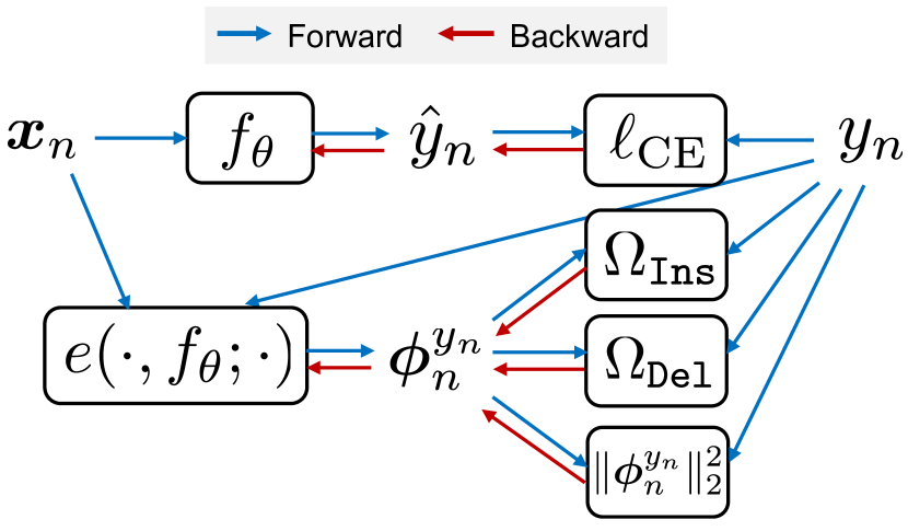
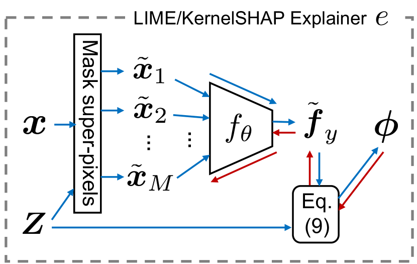
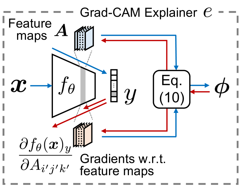
Figure 1: The overview of the forward and backward computations in training using ID-ExpO. (Left) the whole computation flow for each training sample $(\boldsymbol{x}_{n},y_{n})$. The computation flows inside (center) LIME/KernelSHAP and (right) Grad-CAM explainers, respectively. Here, the red double line in Grad-CAM indicates that it computes second-order derivatives when updating predictor $f_{\theta}$ as it uses the gradients w.r.t. feature maps to obtain $\boldsymbol{\phi}$.

Based on the differentiable insertion and deletion metrics, we define insertion and deletion metric-based regularizers that regularize the predictor to maximize the insertion scores and minimize the deletion scores, as follows:

$$\Omega_{\mathtt{Ins}}(\boldsymbol{\phi}^{y},f_{\theta};\boldsymbol{x},y,\boldsymbol{b}) =-\frac{1}{S}\sum_{s=1}^{S}\log f_{\theta}(\alpha_{\mathrm{soft}}(\boldsymbol{x},\boldsymbol{\phi}^{y};\boldsymbol{b},s))_{y},$$ (9)

$$\Omega_{\mathtt{Del}}(\boldsymbol{\phi}^{y},f_{\theta};\boldsymbol{x},y,\boldsymbol{b}) =-\frac{1}{S}\sum_{s=1}^{S}\log\frac{f_{\theta}(\boldsymbol{x})_{y}}{f_{\theta}(\beta_{\mathrm{soft}}(\boldsymbol{x},\boldsymbol{\phi}^{y};\boldsymbol{b},s))_{y}},$$ (10)

where we use $\log f_{\theta}$ instead of using $f_{\theta}$ directly for numerical stability. With the deletion metric-based regularizer, we have attempted three types of formulations. Consequently, (10) can achieve the best performance, as shown in Appendix A of the supplementary material.

In training, for $f_{\theta}$ already trained in a supervised learning manner, we fine-tune it based on the regularizers together with the standard prediction loss. In particular, given $N$ training samples $\{(\boldsymbol{x}_{n},y_{n})\}_{n=1}^{N}$ where $\boldsymbol{x}_{n}\in\mathcal{X}$ and $y_{n}\in\mathcal{Y}$, we solve the following minimization problem by SGD:

$$\mathop{\rm argmin}\limits_{\theta}\sum_{n=1}^{N}\ell_{\mathrm{CE}}(f_{\theta}(\boldsymbol{x}_{n}),y_{n})+\lambda_{1}\Omega_{\mathtt{Ins}}(\boldsymbol{\phi}^{y_{n}}_{n},f_{\theta};\boldsymbol{x}_{n},y_{n},\boldsymbol{b})$$

$$+\lambda_{2}\Omega_{\mathtt{Del}}(\boldsymbol{\phi}^{y_{n}}_{n},f_{\theta};\boldsymbol{x}_{n},y_{n},\boldsymbol{b})+\lambda_{3}\|\boldsymbol{\phi}^{y_{n}}_{n}\|^{2}_{2},$$ (11)

where $\ell_{\mathrm{CE}}(f_{\theta}(\boldsymbol{x}_{n}),y_{n})$ is the cross-entropy loss between prediction $f_{\theta}(\boldsymbol{x}_{n})$ and label $y_{n}$. $\lambda_{1},\lambda_{2}$ and $\lambda_{3}$ are hyperparameters. $\lambda_{1},\lambda_{2}\geq 0$ are weights for those regularizers, respectively. $\|\boldsymbol{\phi}^{y_{n}}_{n}\|^{2}_{2}$ is an L2 regularizer to prevent the divergence of $\boldsymbol{\phi}^{y_{n}}_{n}$, and $\lambda_{3}\geq 0$ is its weight. The left side of Figure 1 illustrates the overview of forward and backward computations in executing (11).

Because $\boldsymbol{\phi}^{y_{n}}_{n}$ is obtained using post-hoc explainer $e(\boldsymbol{x}_{n},f_{\theta};y_{n})$, the implementation of (11) depends on which post-hoc explainer we use. Below we describe the implementations for perturbation-based explainers and gradient-based ones, respectively.

ID-ExpO for Perturbation-Based Explainers.   For an image, the perturbation-based explainers learn interpretable functions that capture the relationship between the predictor’s inputs and outputs using perturbations around the image. The representative methods in the perturbation-based explanation are LIME and KernelSHAP, which calculate pixel-level contributions using the coefficients of linear regression models learned on perturbations around the input image. We illustrate the computation flow of those explainers in the center of Figure 1. First, we partition the image into $D$ super-pixels. Then, we generate $M$ binary random vectors whose $m$th vector is denoted by $\boldsymbol{z}_{m}\in\{0,1\}^{D}$, and its $l$th element indicates whether its corresponding super-pixel is masked ($z_{ml}=0$) or not ($z_{ml}=1$). According to $\boldsymbol{z}_{m}$, we obtain masked perturbed image $\tilde{\boldsymbol{x}}_{m}$ from the original image $\boldsymbol{x}$. Letting $\boldsymbol{Z}=[\boldsymbol{z}_{1},\boldsymbol{z}_{2},\cdots,\boldsymbol{z}_{M}]^{\top}\in\{0,1\}^{M\times D}$ and $\tilde{\boldsymbol{f}}_{y}=[f_{\theta}(\tilde{\boldsymbol{x}}_{m})_{y}]_{m=1}^{M}$, the LIME and KernelSHAP explainers calculate the pixel-level contributions by first solving the weighted least squared problem and then expanding the obtained coefficients into the pixels of the image, as follows:

$$e(\boldsymbol{x},f_{\theta};y)=\mathtt{expand}_{D\rightarrow H\times W}\Big{(}(\boldsymbol{Z}^{\top}\boldsymbol{K}\boldsymbol{Z}+\epsilon\boldsymbol{I}_{D})^{-1}\boldsymbol{Z}\boldsymbol{K}\tilde{\boldsymbol{f}}_{y}\Big{)},$$ (12)

where $\mathtt{expand}_{D\rightarrow H\times W}$ is a function that expands the contribution assigned for each of $D$ super-pixels into the pixels associated with the super-pixel. $\boldsymbol{K}$ is a diagonal matrix of size $M\times M$ whose $(m,m)$-element is the kernel value between a $D$-dimensional all-one vector and $\boldsymbol{z}_{m}$. $\boldsymbol{I}_{D}$ is the identity matrix of size $D$, and $\epsilon\geq 0$ is the hyperparameter of the L2 regularizer. The key difference between LIME and KernelSHAP lies in the kernel function used to compute $\boldsymbol{K}$: LIME uses a cosine kernel, while KernelSHAP uses a Shapley kernel.

ID-ExpO for Gradient-Based Explainers.   One of the most popular gradient-based explainers is Grad-CAM. We illustrate the computation flow of the Grad-CAM explainer on the right side of Figure 1. Grad-CAM obtains non-negative pixel-level contributions by calculating the activation map on the intermediate layers of predictor $f_{\theta}$. Typically, convolutional neural networks are used as the predictors. To compute the activation map, Grad-CAM uses the feature maps in a convolution layer of the CNN predictor, denoted by $\boldsymbol{A}\in\mathbb{R}^{C^{\prime}\times H^{\prime}\times W^{\prime}}$ where $C^{\prime}$, $H^{\prime}$ and $W^{\prime}$ are the number of channels, height, and width of the feature maps, respectively. Also, it calculates the gradient of the output of the CNN predictor with respect to each element of the feature maps, i.e., $\frac{\partial f_{\theta}(\boldsymbol{x})_{y}}{\partial A_{i^{\prime}j^{\prime}k^{\prime}}}$. Using them, the Grad-CAM explainer calculates the activation map $\boldsymbol{M}\in\mathbb{R}_{\geq 0}^{H^{\prime}\times W^{\prime}}$ for label $y$ followed by the pixel-level importance from $\boldsymbol{M}$, as follows:

$$e(\boldsymbol{x},f_{\theta};y) =\mathtt{expand}_{H^{\prime}\times W^{\prime}\rightarrow H\times W}\Bigg{(}\underbrace{\mathrm{ReLU}\Big{(}\sum_{i^{\prime}=1}^{C^{\prime}}\omega^{y}_{i^{\prime}}\boldsymbol{A}_{i^{\prime}}\Big{)}}_{=\boldsymbol{M}}\Bigg{)},$$ (13)

$$\omega^{y}_{i^{\prime}} =\frac{1}{H^{\prime}W^{\prime}}\sum_{j^{\prime}=1}^{H^{\prime}}\sum_{k^{\prime}=1}^{W^{\prime}}\frac{\partial f_{\theta}(\boldsymbol{x})_{y}}{\partial A_{i^{\prime}j^{\prime}k^{\prime}}},$$ (14)

where $\mathtt{expand}_{H^{\prime}\times W^{\prime}\rightarrow H\times W}$, as with that in (12), expands $(j^{\prime},k^{\prime})$-element of the activation map $\boldsymbol{M}$ into its corresponding pixels on the image. $\mathrm{ReLU}$ is the rectified linear unit.

For Data Other Than Images.   ID-ExpO is also available in the cases that an input data is $Q$-dimensional vector $\boldsymbol{x}\in\mathcal{X}\subseteq\mathbb{R}^{Q}$, e.g., text classification and tabular classification, whose $q$th dimension represents the $q$th feature value. In the cases, we replace $ijk$ and $jk$ in (1)–(10) specifying indices in an image with $q\in\{1,2,\cdots,Q\}$. Also, the maximum value of $S$ becomes $Q$ instead of $HW$.

Missingness Bias.   When producing explanations using perturbation-based explainers and evaluating explanations by insertion/deletion metrics, we mask a part of the pixels in the input image. This input masking causes a problem called missingness bias, which means that the masked images are out of training input distribution. Jain et al. reported that the missingness bias causes the explanations by LIME not to be aligned with human intuition, and training the model with random masking augmentation mitigates the problem [83]. Our regularizers, (9) and (10), evaluate the predictive loss, $\log f(\cdot)$, in which a part of the input pixels is masked, which has similar effects with the training with random masking augmentation. Therefore, our regularizers can naturally deal with the missingness bias.

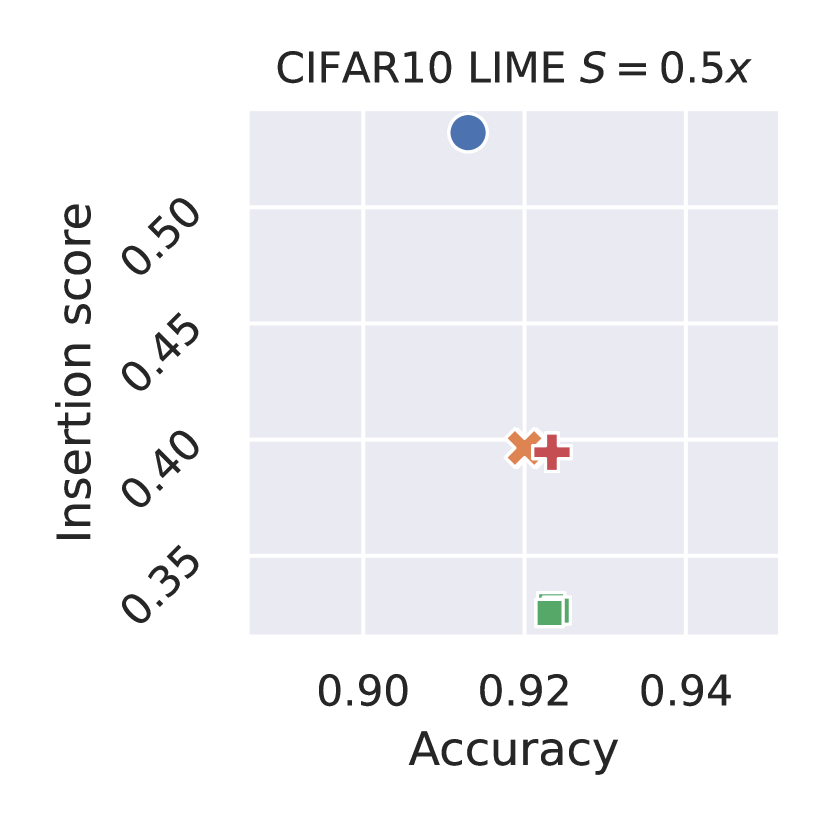
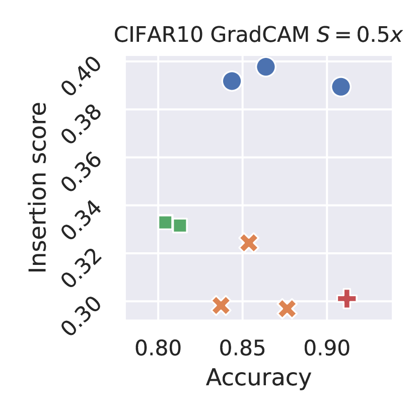
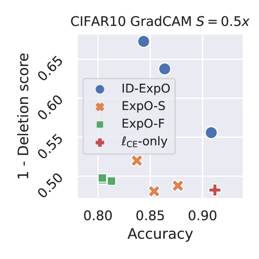
Figure 2: Mean insertion and mean one-minus-deletion scores against accuracy on CIFAR-10 in case of $S=0.5\cdot HW$. The top row shows the results on LIME, while the bottom row shows the results on Grad-CAM. Each point indicates the result for the hyperparameters chosen based on (15) with a different accuracy weight $\eta\in\{0.5,1.0.\cdots,3.0\}$ (different $\eta$ values can be plotted in the same location). The higher those scores, the better.

4 Experiments

We conducted experiments on two image datasets and six tabular datasets to evaluate the effectiveness of our ID-ExpO in the case of using LIME, KernelSHAP and Grad-CAM as post-hoc explainers. For page limitation, we report the results of the image classification task in this section and those of the tabular classification task in Appendix C of the supplementary material. The experiments were done using the codes written in PyTorch v.1.13 on a computer consisting of an Intel Xeon Platinum 8360Y, an NVIDIA A100 SMX4 GPU, and memories of 512GB.

Comparing Methods.   We compared the proposed method (ID-ExpO) with the following methods: stability-aware explanation-based optimization (ExpO-S), fidelity-aware explanation-based optimization (ExpO-F), and fine-tuning without explanation regularizers ($\ell_{\mathrm{CE}}$-only). ExpO-S and ExpO-F were based on the study [60]. They aim to improve the stability and fidelity of explanations produced by perturbation-based explainers such as LIME. ExpO-S learns the predictor with a regularizer so that the outputs of the predictor do not change for neighborhoods of the input. ExpO-F learns the predictor with another regularizer so that the outputs of the predictor for the neighborhoods are fitted with a local linear function. Since the original ExpO-S and ExpO-F are not developed for image data, we extended the ExpO-S and ExpO-F to apply to both image and tabular data, as described in Appendix B.1 of the supplementary material. $\ell_{\mathrm{CE}}$-only learns the predictor without any regularizer of explanation, which is equivalent to optimizing (11) with $\lambda_{1}=\lambda_{2}=\lambda_{3}=0$.

Evaluation.   We quantitatively assessed the proposed method and the comparing ones in terms of predictive accuracy, insertion score (1) and deletion score (3). Here, we set $S$ to 30% or 50% of the number of features (pixels), which is the same value as that used in our regularizers (9) and (10). For readability, we also use one-minus-deletion score instead of the deletion score, which is calculated by subtracting the deletion score from one. Furthermore, to check if the proposed method can improve other faithfulness metrics, which are not optimized directly, we also assessed explanations in sensitivity-$n$ [74], which evaluates, when $n$ features are randomly removed, how much the sum of the contributions of the removed features correlates the decrease of the predicted confidence. Here, we set to $n=300$.

As the criterion used for model selection and monitoring the proceeding of the training, we used the validation score function defined as follows:

$$\mathrm{valscore}(f_{\theta};\eta)=\eta\cdot\mathtt{Acc}(f_{\theta})+\mathtt{Ins}(f_{\theta})+1-\mathtt{Del}(f_{\theta}),$$ (15)

where $\mathtt{Acc}(f_{\theta})$, $\mathtt{Ins}(f_{\theta})$ and $\mathtt{Del}(f_{\theta})$ indicate predictive accuracy, average insertion score and average deletion score for the validation set on predictor with current parameters $f_{\theta}$, respectively. $\eta\geq 0$ is an accuracy weight used to control the ratio of predictive and explanatory capabilities. Unless otherwise noted, we set $\eta=2$, indicating that the predictive and explanatory capabilities are equally evaluated.

4.1 Image Classification

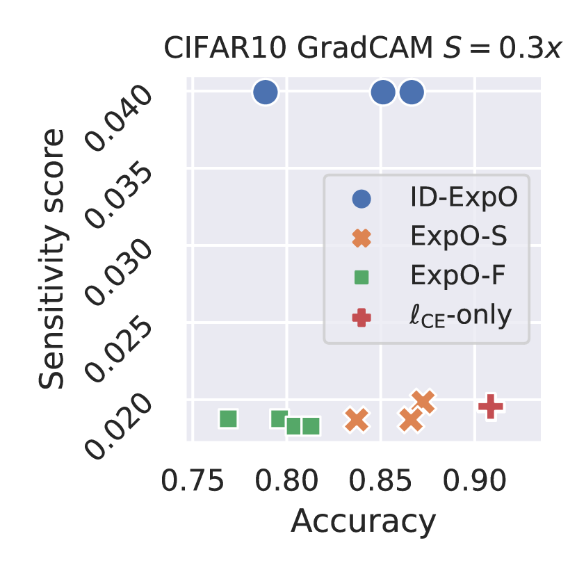
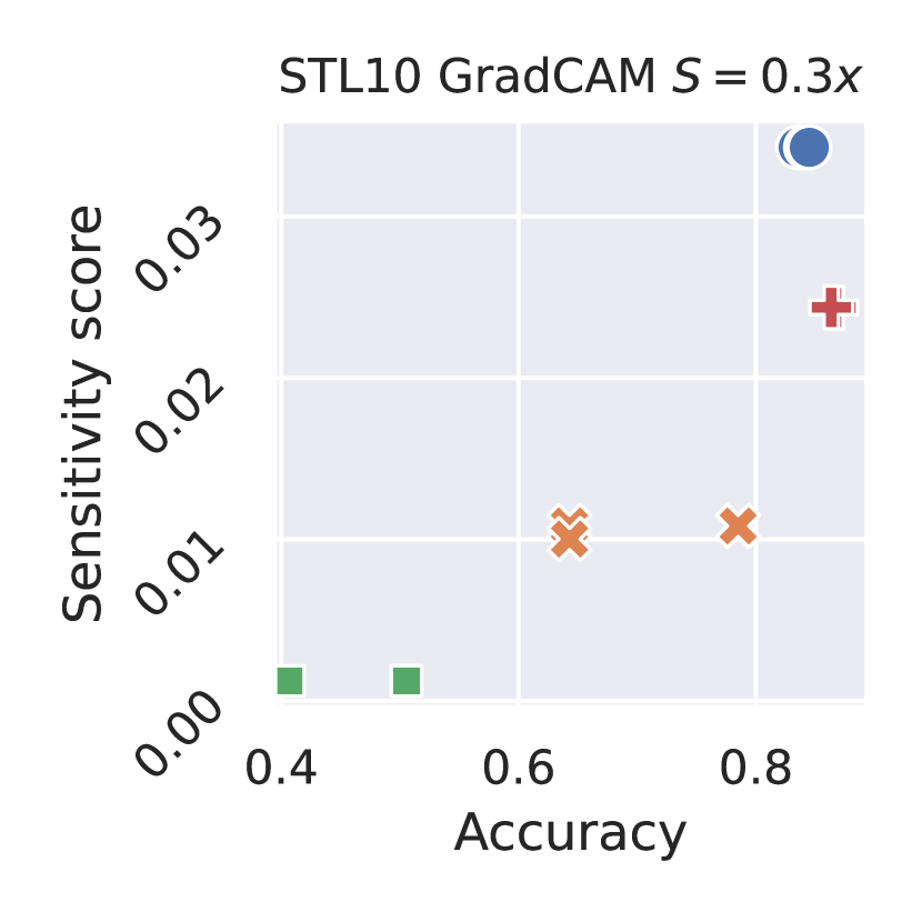
Figure 3: Mean sensitivity-$n$ scores against accuracy on CIFAR-10 (left) and STL-10 (right) in case of $S=0.3\cdot HW$. The higher those scores, the better.

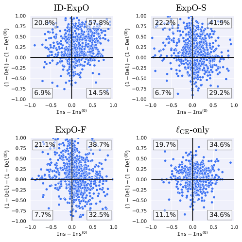
Figure 4: The differences in the insertion and one-minus-deletion scores between before and after fine-tuning predictors with Grad-CAM using each method for 1,000 randomly selected individual test samples on CIFAR-10. $\mathtt{Ins}$ and $\mathtt{Del}$ indicate the mean insertion and deletion scores over the test set when using the predictors after fine-tuning, while $\mathtt{Ins}^{(0)}$ and $\mathtt{Del}^{(0)}$ indicate those before fine-tuning. The percentage in each quadrant is the ratio of samples located in the quadrant.

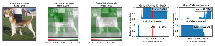
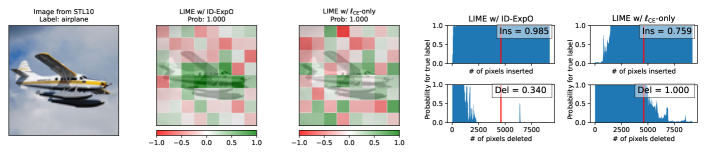
(a)

(b)

(c)

(d)

(e)

Figure 5: Examples of the produced explanations on STL-10. The first row shows the results by Grad-CAM, while the other shows the results by LIME. Each row illustrates (a) an input image, (b) (c) the heatmaps of the explanations by the explainers with ID-ExpO and $\ell_{\mathrm{CE}}$-only, and (d) (e) the insertion score (top) and the deletion score (bottom) for those explanations in the case of $S=0.5\cdot HW$, which means that the scores are the blue areas to the left of red vertical lines.

Datasets.   We used two standard benchmark image classification datasets, CIFAR-10 [84] and STL-10 [85]. CIFAR-10 contains 60,000 color images with a resolution of 32x32, divided into ten distinct classes. There are originally 50,000 labeled images for training and 10,000 labeled images for testing. In our experiment, we left 10,000 images in the original training set for validation. STL-10 consists of color images with a resolution of 96x96, with ten classes and 1,300 images per class. It originally provides 5,000 labeled images for training and 8,000 labeled images for testing. In our experiment, we left 500 images in the original training set for validation.

Implementation.   We used ResNet-18 [86] as a predictor. We trained it in advance on each training set in the standard supervised learning manner with the data augmentation of random horizontal flipping and random cropping. For the LIME explainer, we first partitioned the image into square-shaped super-pixels of different sizes depending on the dataset. We used the super-pixels with the size of 4x4 or the 32x32-pixel images of CIFAR-10, while we used the super-pixels with the size of 12x12 for the 96x96-pixel images of STL-10. Therefore, the numbers of super-pixels were set to $D=(32/4)^{2}=64$ for CIFAR-10 and $D=(96/12)^{2}=64$ for STL-10. We also used $D$ as the constant to increment $s$ because the pixel contributions on a super-pixel are the same. We generated $M=200$ perturbations and were set to $\epsilon=0.01$ in (12). For the Grad-CAM explainer, we used the feature maps of the conv3_x and conv4_x building blocks in ResNet-18 for CIFAR-10 and STL-10, respectively. The sizes of the feature maps are 8x8 for CIFAR-10 and 6x6 for STL-10. Depending on those sizes, we decided $s$ to increment by 16 for CIFAR-10 and 256 for STL-10.

The hyperparameters in ID-ExpO are $\lambda_{1}$, $\lambda_{2}$ and $\lambda_{3}$ in (11), and temperature parameter $T$. Throughout the experiments in this paper, we used the same value $\lambda_{12}$ for $\lambda_{1}$ and $\lambda_{2}$. We determined the best hyperparameter values in the ranges of $\lambda_{12}\in\{0.1,0.01,0.001\}$ and $\lambda_{3}\in\{0.001,0\}$ based on (15). $T$ in soft step function $r$ has a role that controls its value not to be nearly equal to zero or one. Since the appropriate value of $T$ is different among samples, for each sample, we determined it as $T=\left(\frac{1}{\#(\boldsymbol{\phi})-1}\left(\max(\boldsymbol{\phi})-\min(\boldsymbol{\phi})\right)\right)^{-1}$, where $\#(\boldsymbol{\phi})$ is the number of elements with non-duplicated values in $\boldsymbol{\phi}$. The hyperparameter in ExpO-S and ExpO-F, the strength of their own regularizer, is determined as the best one in the range of $\{0.1,0.01,0.001\}$ based on (15). There is no hyperparameter specific for $\ell_{\mathrm{CE}}$-only. As the optimizer, we used SGD optimizer with a mini-batch size of 128, momentum factor of 0.9, weight decay of 0.0005, and Nesterov momentum. Its learning rate was determined based on (15) within the range of $\{10^{-4},10^{-5}\}$. The training continued until 50 epochs were reached or the value of $\mathrm{valscore}(f_{\theta};2)$ does not gain for ten consecutive epochs.

4.1.1 Results

Figure 2 shows the insertion and one-minus-deletion scores against predictive accuracy on CIFAR-10. Here, those scores are averaged over all the samples in the test set. On all the results, ID-ExpO achieved the best insertion and deletion scores. This fact indicates that our insertion and deletion metric-based regularizers used in ID-ExpO are effective, although the stability-aware regularizer in ExpO-S and the fidelity-aware regularizer in ExpO-F are not suitable for improving those scores. With the predictive accuracy, ID-ExpO was comparable with $\ell_{\mathrm{CE}}$-only when controlling $\eta$ in (15) to achieve the highest accuracy, e.g., $\eta=3$ while keeping that the insertion and deletion scores of ID-ExpO were better than those of $\ell_{\mathrm{CE}}$-only. Similar results were observed in the case of $S=0.3\cdot HW$ and on STL-10, as shown in Appendix B.2 of the supplementary material.

As described in Section 3.1, the regularizers in ID-ExpO can naturally make predictors robust to the missingness bias. The missingness bias can undeservedly make the insertion and deletion scores of the comparing methods better than those of ID-ExpO because the predictors sensitive to the bias can change prediction largely even if unimportant pixels are inserted in or masked out. Therefore, the fact that ID-ExpO achieved the best insertion and deletion scores indicates that the regularizers in ID-ExpO are effective in improving the faithfulness of explanations.

To investigate the impact of the proposed and the existing optimization on a faithfulness metric other than insertion/deletion metrics, we also evaluate the produced explanations in sensitivity-$n$ metric in Figure 3, which ID-ExpO does not optimize directly. The figure shows that ID-ExpO consistently improved the sensitivity-$n$ metric on CIFAR-10 and STL-10, while ExpO-S and ExpO-F did not. This result indicates that ID-ExpO does not overfit the insertion and deletion metrics, and it can contribute to improving the faithfulness of explanations from various perspectives.

Figure 4 shows how much the insertion and deletion scores of individual samples changed before and after fine-tuning the predictor based on each method. In ID-ExpO, ExpO-S, ExpO-F and $\ell_{\mathrm{CE}}$-only, 57.8%, 41.9%, 38.7% and 34.6% of samples were located in the first quadrant, respectively. Since the first quadrant means that the changes of the insertion and one-minus-deletion scores are both positive, we found that ID-ExpO was most effective in making explanations more faithful. Conversely, the ratios of the samples located in the third quadrant, which means that samples became less faithful, were 6.9%, 6.7%, 7.7% and 11.1%, respectively. We also found that the possibility that ID-ExpO worsens the faithfulness of the explanations is relatively low.

In Figure 5, we visualize the produced explanations for the predictors trained using ID-ExpO and $\ell_{\mathrm{CE}}$-only, and show the distributions of the insertion and deletion metrics of the explanations. More results are shown in Appendix B.3 of the supplementary material. Here, we show the examples in which correct prediction was made. As shown in Figures 5(d) and 5(e), we found that the distributions of the insertion and deletion metrics were substantially different between ID-ExpO and $\ell_{\mathrm{CE}}$-only. The result indicates that our insertion and deletion metric-based regularizers positively affect those distributions as we expected. Also, as shown in Figures 5(b) and 5(c), we found that the explanations themselves were different between them. In particular, in the heatmap explanations for ID-ExpO (Figure 5(b)), large positive contributions were assigned to a part of super-pixels that captures the object of the class label well. This is because the evaluation of the insertion and deletion scores in our regularizers is truncated at 30% or 50% of the number of pixels. The results indicate that ID-ExpO can change the explanations to preferentially assign larger positive contributions to the pixels strongly affecting the prediction to improve those metrics.

5 Conclusion

We proposed an explanation-based optimization that learns machine learning predictors, such as DNNs, with insertion and deletion metrics-aware regularizers. By fine-tuning the predictors based on the proposed method, we confirmed that a wide range of explainers, including perturbation-based and gradient-based, can produce explanations faithful to the predictors’ behaviors. In future work, we will further verify the effectiveness of our insertion and deletion metrics-aware regularizers by applying them for the faithfulness of the explanations by inherently interpretable models [57] and parameterized explainers [87].

 Supplementary Material:
Explanation-Based Training with Differentiable Insertion/Deletion Metric-Aware Regularizers

 

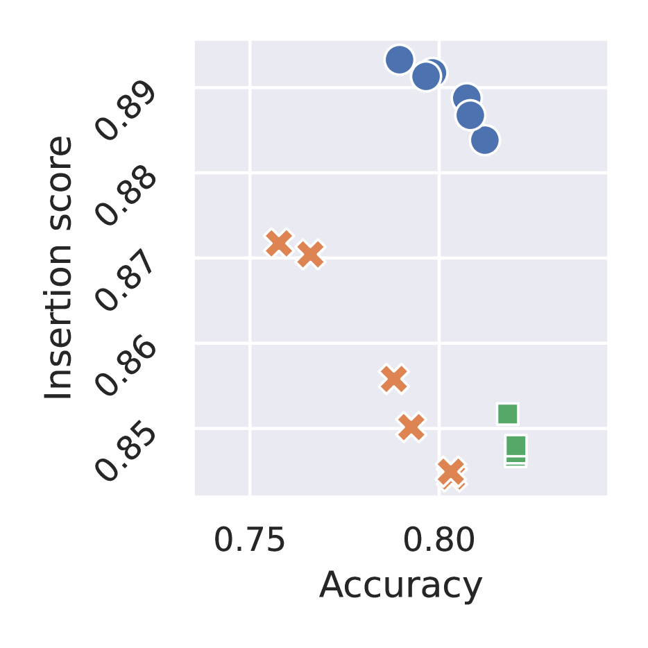
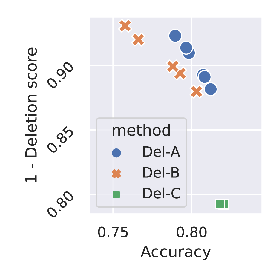
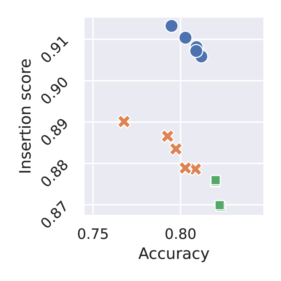
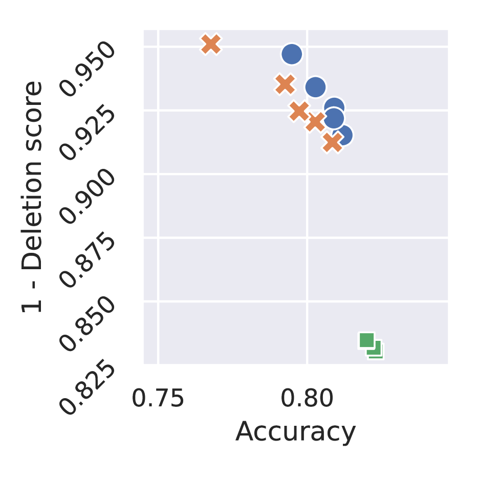
Figure A.1: Mean insertion and mean one-minus-deletion scores against mean accuracy averaged over six tabular datasets when using LIME as the explainer among three types of deletion metric-aware regularizers. Each point has a different accuracy weight $\eta\in\{0.5,1.0.\cdots,3.0\}$. Figures of the first two columns are the results at $S=0.3\cdot HW$, while those of the other columns are the results at $S=0.5\cdot HW$. Higher those scores, the better.

Appendix A Comparison Among Different Types of Deletion Metric-Based Regularizers

We formalized three types of deletion metric-based regularizers, as follows:

$$\mbox{\bf Del-A}:\quad\Omega_{\mathtt{Del}}(\boldsymbol{\phi}^{y},f_{\theta};\boldsymbol{x},y,\boldsymbol{b}) =-\frac{1}{S}\sum_{s=1}^{S}\log\frac{f_{\theta}(\boldsymbol{x})_{y}}{f_{\theta}(\beta_{\mathrm{soft}}(\boldsymbol{x},\boldsymbol{\phi}^{y};\boldsymbol{b},s))_{y}},$$ (A.1)

$$\mbox{\bf Del-B}:\quad\Omega_{\mathtt{Del}}(\boldsymbol{\phi}^{y},f_{\theta};\boldsymbol{x},y,\boldsymbol{b}) =\frac{1}{S}\sum_{s=1}^{S}\log f_{\theta}(\beta_{\mathrm{soft}}(\boldsymbol{x},\boldsymbol{\phi}^{y};\boldsymbol{b},s))_{y},$$ (A.2)

$$\mbox{\bf Del-C}:\quad\Omega_{\mathtt{Del}}(\boldsymbol{\phi}^{y},f_{\theta};\boldsymbol{x},y,\boldsymbol{b}) =-\frac{1}{S}\sum_{s=1}^{S}\log\left(1-f_{\theta}(\beta_{\mathrm{soft}}(\boldsymbol{x},\boldsymbol{\phi}^{y};\boldsymbol{b},s))_{y}\right),$$ (A.3)

where Del-A is what the proposed method employs. Del-B is similar to Del-A but does not have the term improving the prediction for the original input. Del-C is similar to Del-B but is formalized like the term for negative class in the binary cross entropy loss.

Figure A.1 shows the insertion and one-minus-deletion scores of the three formulations. We found that Del-A achieved the best balance of the accuracy and insertion/one-minus-deletion score.

Appendix B On Experiments on Image Datasets

B.1 Modified Version of ExpO-S and ExpO-F

The original ExpO-Stability (ExpO-S for short) and ExpO-Fidelity (ExpO-F for short) aim at making predictions and their corresponding explanations robust to slight changes in the feature values of the input, respectively [60]. The authors stated that the ExpO-F did not evaluate for non-semantic features, such as images, as the fidelity metric is not appropriate for the non-semantic features [60, Appendix A.8]. Therefore, while keeping the idea of the original ExpO-F, we modified it to apply it to image data. In particular, we utilize the same approach to LIME for image data, which we describe in Section 3.1, as the fidelity regularizer mimics the derivation of the explanations produced by LIME. Below we use the same notation of the variables in Section 3.1. First, for a given training sample $(\boldsymbol{x},y)$, we obtain a LIME explanation $\boldsymbol{\phi}^{y}$ by applying (9). Then, since $\boldsymbol{\phi}^{y}$ is the coefficients of a local linear model around input $\boldsymbol{x}$, we can calculate the fidelity-aware regularizer based on the original ExpO-F as follows:

$$\Omega_{\mathtt{Fidelity}}(\boldsymbol{\phi}^{y},f_{\theta};\boldsymbol{x},y,\{\boldsymbol{z}_{m}\}_{m=1}^{M},\boldsymbol{K})=\frac{1}{M}\sum_{m=1}^{M}\boldsymbol{K}_{mm}(f_{\theta}(\tilde{\boldsymbol{x}}_{m})_{y}-\boldsymbol{\phi}^{y}{}^{\top}\boldsymbol{z}_{m})^{2}.$$ (A.4)

where $\boldsymbol{z}_{m}\in\{0,1\}^{D}$ is the $m$th binary random vector to mask $D$ super-pixels, $f_{\theta}(\tilde{\boldsymbol{x}}_{m})_{y}$ is the predicted probability of label $y$ for perturbed mask image $\tilde{\boldsymbol{x}}_{m}$, $\boldsymbol{K}_{mm}$ is the value of a cosine kernel between a $D$-dimensional all-one vector and $\boldsymbol{z}_{m}$.

The original ExpO-S can be applied to numerical features and non-semantic features as it calculates the differences between the prediction for the original input and that for the perturbed input, in which Gaussian perturbations are added to the features of the input. However, for the consistency of evaluation, we modified the original ExpO-S to perturb the input with binary random mask vectors $\boldsymbol{Z}$. In particular, we calculate the stability-aware regularizer as follows:

$$\Omega_{\mathtt{Stability}}(\boldsymbol{\phi}^{y},f_{\theta};\boldsymbol{x},y,\{\tilde{\boldsymbol{x}}_{m}\}_{m=1}^{M},\boldsymbol{K})=\frac{1}{M}\sum_{m=1}^{M}\boldsymbol{K}_{mm}(f_{\theta}(\tilde{\boldsymbol{x}}_{m})_{y}-f_{\theta}(\boldsymbol{x}))^{2}.$$ (A.5)

B.2 All Quantitative Results on Image Datasets

Figure A.2 shows the insertion and the one-minus-deletion scores against the accuracy on each image dataset. On all the explainers and the datasets except Grad-CAM on STL-10 (Figure A.2(D)), we found that the insertion and one-minus-deletion scores of ID-ExpO are superior to those of the other methods. With the accuracy, by putting emphasis on the accuracy, i.e., by setting $\eta=3$, we found that ID-ExpO in the case of $S=0.5\cdot HW$ could keep comparable or slightly low accuracy compared to the others, while the highest insertion and one-minus-deletion scores. However, in the case of $S=0.3\cdot HW$, we found that the accuracy of ID-ExpO was lower than the other methods and the accuracy of ID-ExpO in the case of $S=0.5\cdot HW$. The setting of $S=0.3\cdot HW$ means that our insertion and deletion metric-aware regularizers force the predictor to use only 30% of the pixels in an image in prediction. The result indicates that the regularization was too strong to predict correctly for the image datasets.

(A) LIME on CIFAR-10

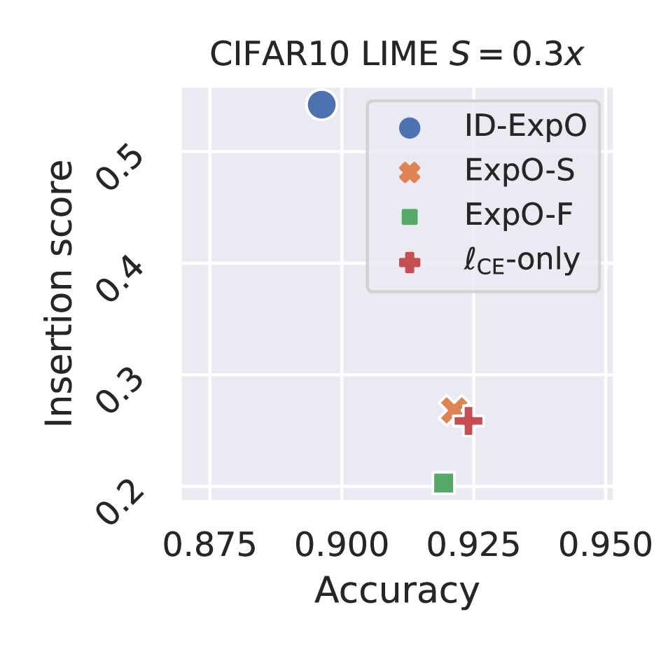
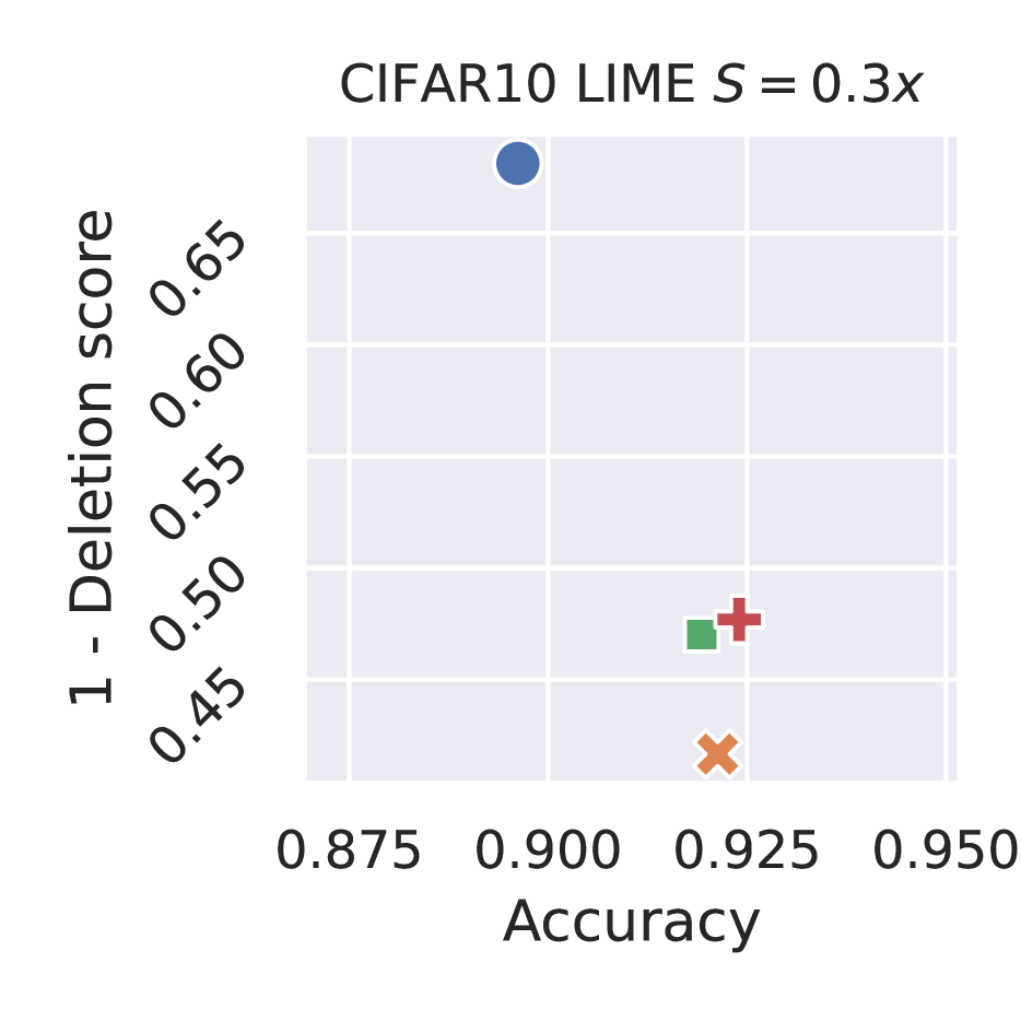
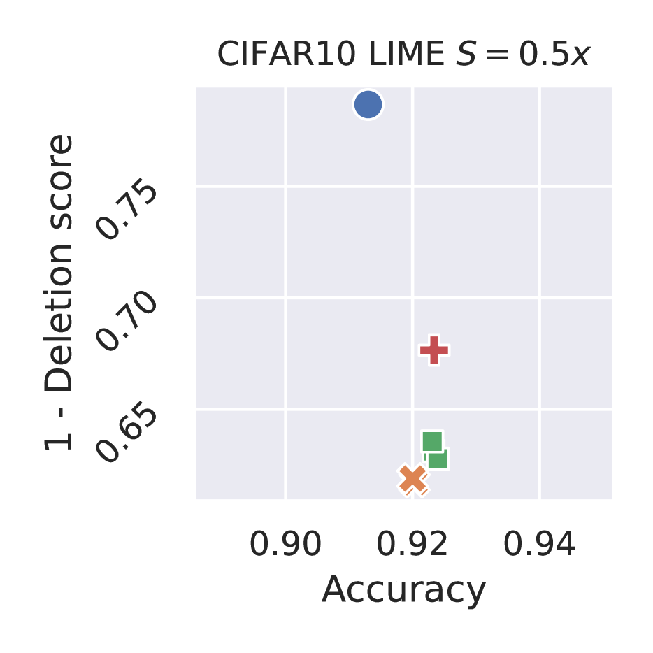
(B) Grad-CAM on CIFAR-10

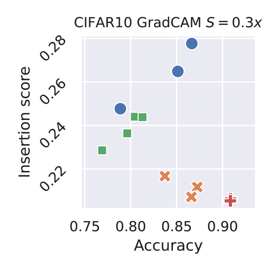
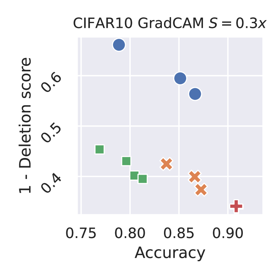
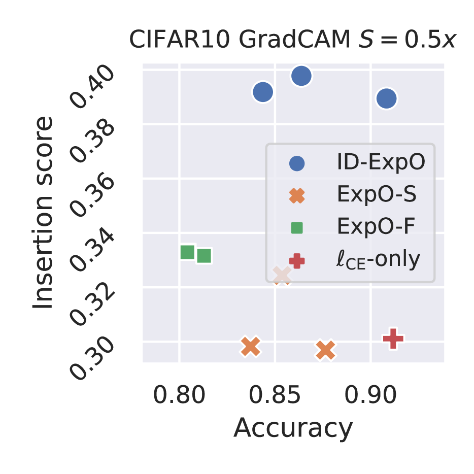
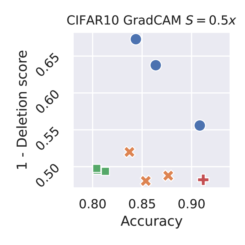
(C) LIME on STL-10

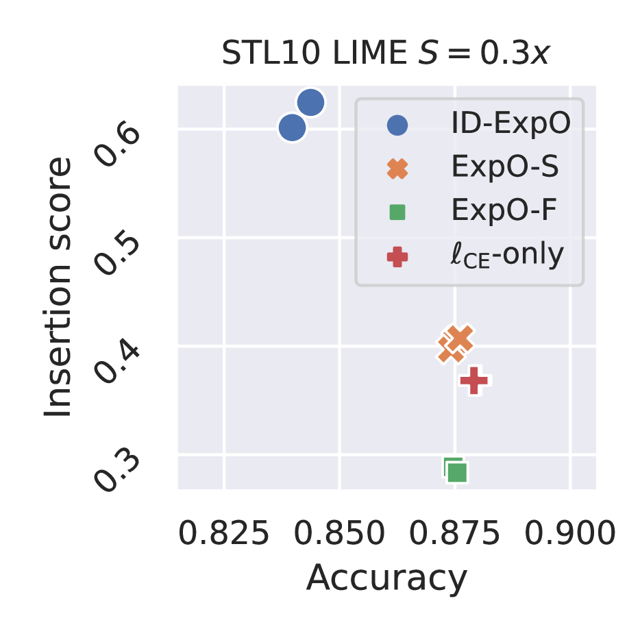
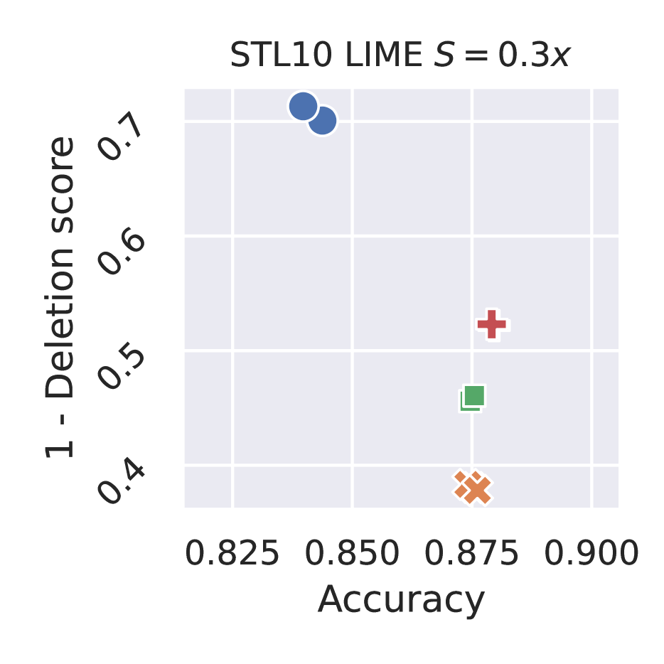
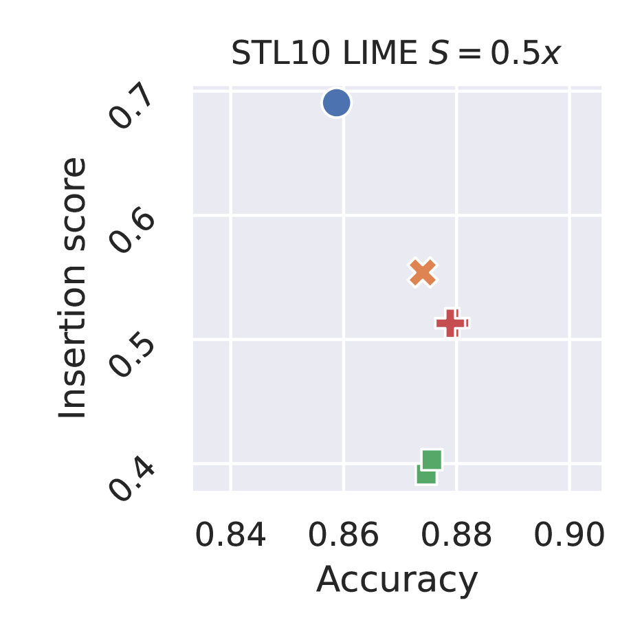
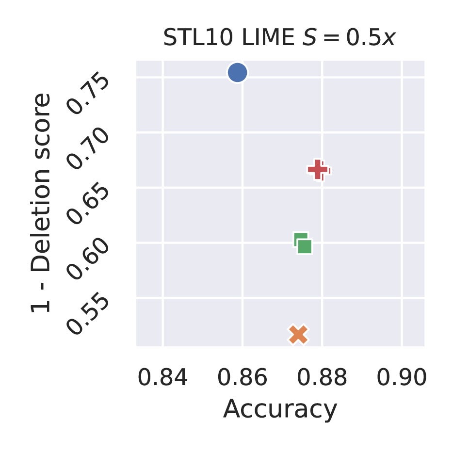
(D) Grad-CAM on STL-10

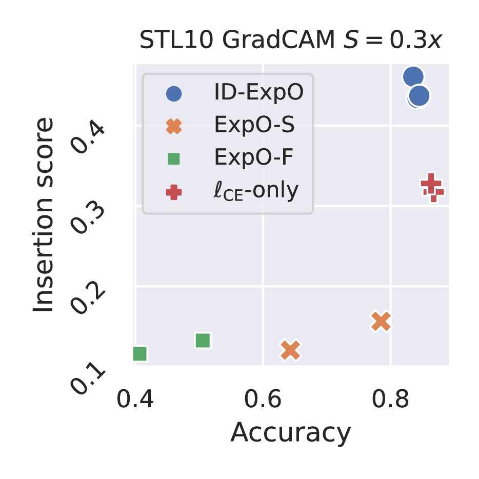
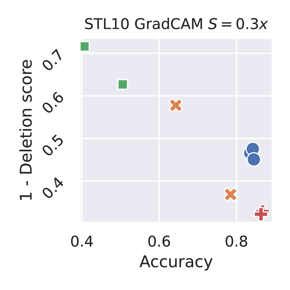
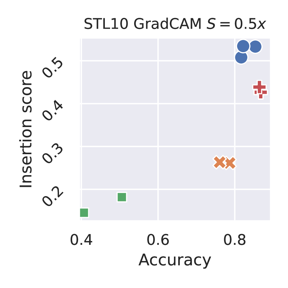
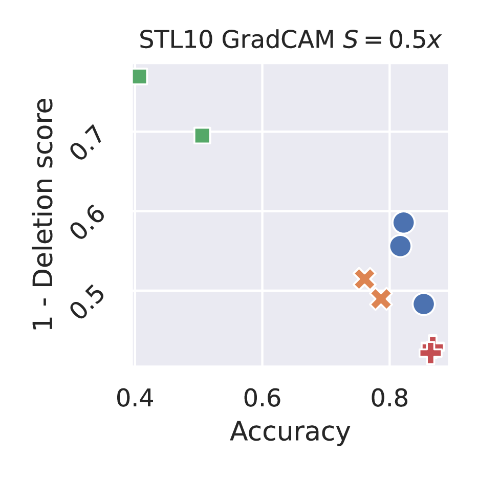
Figure A.2: Mean insertion and mean one-minus-deletion scores against accuracy on each image dataset. Each row indicates a different pair of an explainer and a dataset. The first two columns show the results when $S=0.3\cdot HW$, while the last two columns show the results when $S=0.5\cdot HW$. Each point indicates the result for the hyperparameters chosen based on (11) with a different accuracy weight $\eta\in\{0.5,1.0.\cdots,3.0\}$ (different $\eta$ values can be plotted in the same location). Higher those scores, the better.

B.3 Additional Examples of Produced Explanations on Image Datasets

Figures A.3 and A.4 show additional visualization examples of the produced explanations on image datasets when the insertion and deletion scores of the explanations were improved by using ID-ExpO. Overall, compared to the explanations of $\ell_{\mathrm{CE}}$-only, the explanations of ID-ExpO had the tendency that large positive contributions were assigned to a part of super-pixels that captures the object of the class label well.

(A) LIME on CIFAR-10 ($S=0.5\cdot HW$)

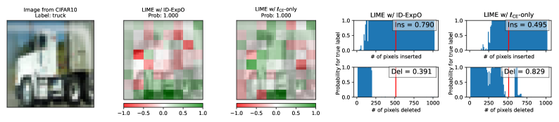
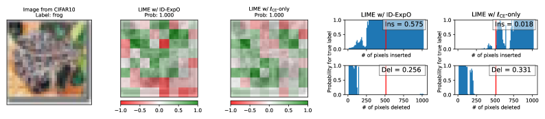
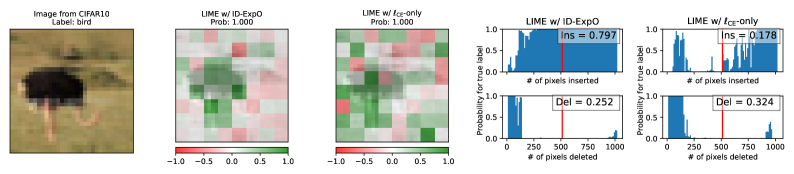
(B) Grad-CAM on CIFAR-10 ($S=0.5\cdot HW$)

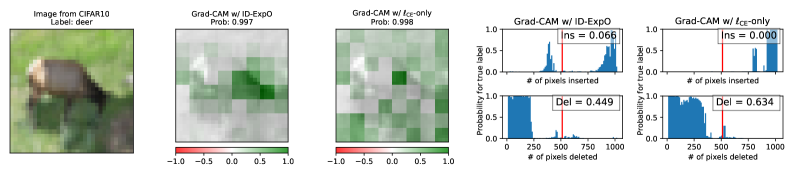
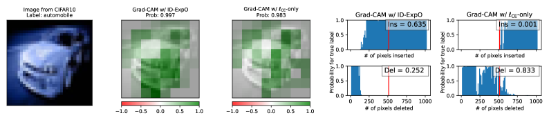
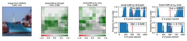
(a)

(b)

(c)

(d)

(e)

Figure A.3: Examples of the produced explanations on CIFAR-10. Each row illustrates (a) an input image, (b) (c) the heatmaps of the explanations by the explainers with ID-ExpO and $\ell_{\mathrm{CE}}$-only, and (d) (e) the insertion score (top) and the deletion score (bottom) for those explanations in the case of $S=0.5\cdot HW$, which means that the scores are the blue areas to the left of red vertical lines.

(A) LIME on STL-10 ($S=0.5\cdot HW$)

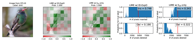
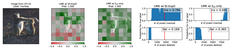
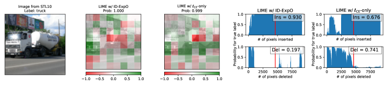
(B) Grad-CAM on STL-10 ($S=0.5\cdot HW$)

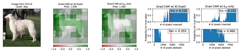
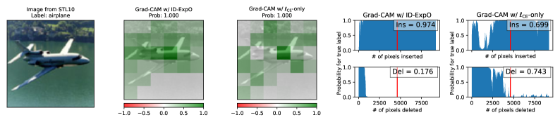
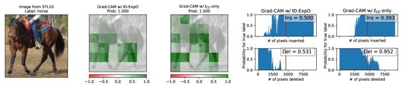
(a)

(b)

(c)

(d)

(e)

Figure A.4: Examples of the produced explanations on STL-10. How to read the figures is the same as Figure A.3.

Appendix C Experiments on Tabular Datasets

C.1 Tabular Datasets

We used six tabular classification datasets with numerical features from OpenML dataset repository [88]: collins, mfeat-fourier, one-hundred-plants-shape, qsar-biodeg, steel-plates-fault, and wine-quality-red. Table A.1 shows the numbers of samples, features and classes of each tabular dataset. For each dataset, we created five sets, each of which consists of training, validation and test sets, by randomly dividing the dataset in the ratio of 70%, 10% and 20%. We standardized each feature value using the training set.

Table A.1: Specification of tabular datasets.

Dataset	# samples	# features	# classes
collins	500	23	2
mfeat-fourier	2,000	77	10
one-hundred-plants-shape	1,600	65	100
qsar-biodeg	1,055	42	2
steel-plates-fault	1,941	28	7
wine-quality-red	1,599	12	6

C.2 Implementation Details for Tabular Datasets

We used a multilayer perceptron (MLP) with two hidden layers of 256 units and ReLU activation functions as a predictor, which was trained on the training set of each dataset in advance in the standard supervised learning manner. We used LIME and KernelSHAP with the same hyperparameter setting as the LIME for the image classification as explainers. Since there is no bunch of features like a super-pixel, we directly calculated the contributions of individual features in (12). We did not use Grad-CAM because it is impossible to associate the features with the activation maps of the intermediate layers of the MLP. The optimizer is the same as that for image classification, except we chose the learning rate in the range of $\{0.01,0.001\}$. The training continued until 200 epochs were reached or the value of $\mathrm{valscore}(f_{\theta};2)$ does not gain for 20 consecutive epochs.

C.3 Results of Tabular Datasets

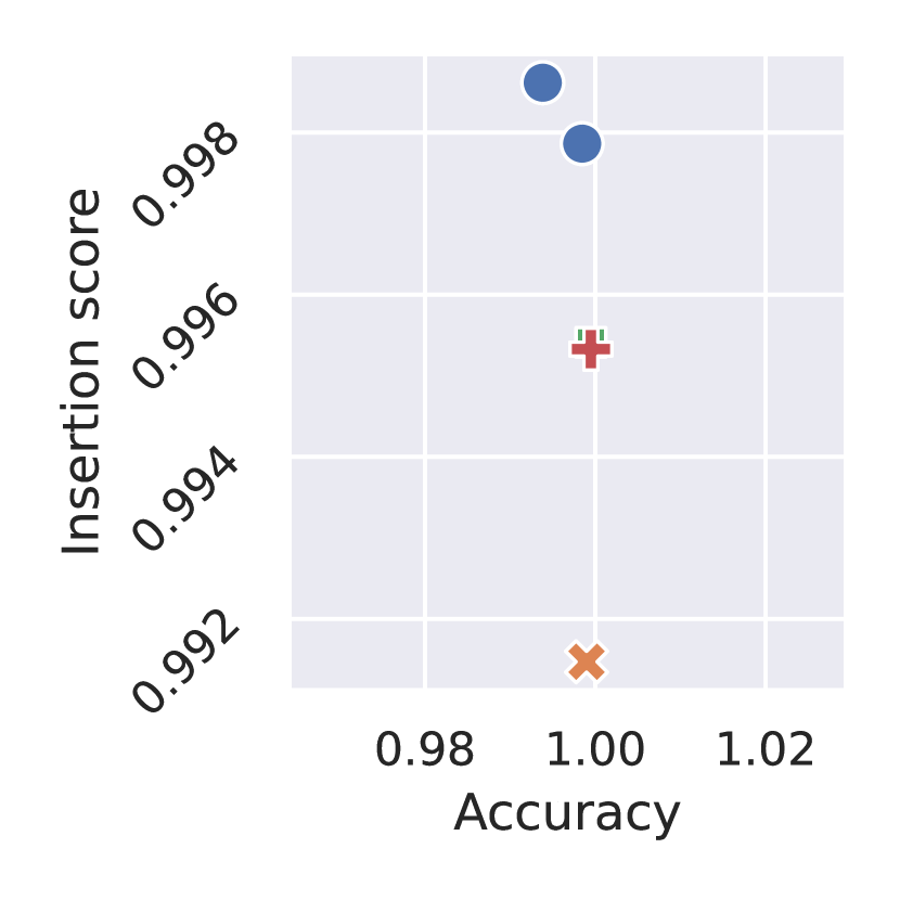
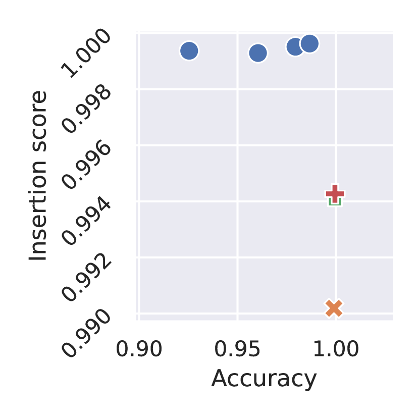
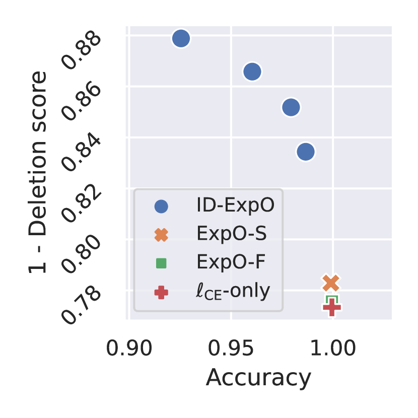
Figure A.5: Mean insertion and mean one-minus-deletion scores against accuracy on steel-plates-fault dataset in case of $S=0.3\cdot Q$. The scores are averaged over the five training/validation/test sets. The first two columns show the results on LIME, while the other shows the results on KernelSHAP.

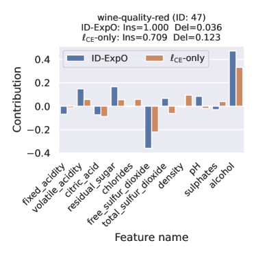
Figure A.6: Feature contributions on a sample in wine-quality-red dataset.

Figure A.5 shows the insertion and one-minus-deletion scores against accuracy on steel-plates-fault dataset. To test the differences among the methods for each evaluation metric, we performed a paired t-test at 5% level for the results with $\eta=3$. As a result, in the case of using LIME, ID-ExpO achieved the highest insertion and one-minus-deletion scores, and there was no statistical accuracy difference among the methods. In the case of using KernelSHAP, although the insertion and one-minus-deletion scores of ID-ExpO were the highest, its accuracy was superior to the comparing methods. LIME and KernelSHAP are similarly formalized as linear regression models. The main difference between them is the kernel functions in (12). Since the Shapley kernel used in KernelSHAP often outputs extremely small values, resulting in unstable calculation in (12), it may have adversely affected the accuracy. As shown in Appendix C.4, similar results were observed on the other tabular datasets.

To analyze how the explanations changed by employing ID-ExpO, we visualize the feature contributions by LIME with ID-ExpO and $\ell_{\mathrm{CE}}$-only. We show a typical example in the wine-quality-red dataset in Figure A.6. In many samples, including this, we found that ID-ExpO tended to bring larger positive or negative feature contributions than $\ell_{\mathrm{CE}}$-only, although LIME for both has the same setting. This is because that ID-ExpO adjusts the predictor’s behaviors so that important features are taken into account early in the calculation of the insertion and deletion metrics. Since the explanation with such feature contributions makes features that users should focus on more clear, ID-ExpO can be effective in producing explanations that are easy to understand for the users.

C.4 All Quantitative Results on Tabular Datasets

Figures A.7–A.9 show the insertion and the one-minus-deletion scores against the accuracy on the six tabular datasets. On all the datasets, ID-ExpO outperformed the others in terms of the insertion and the one-minus-deletion scores for any in the range of $\eta$. With the accuracy, by putting emphasis on the accuracy, i.e., by setting $\eta=3$, we found that ID-ExpO could keep comparable or slightly low accuracy compared to the others, while the highest insertion and one-minus-deletion scores. However, in some cases of using KernelSHAP, e.g., Figures A.8(C) and A.9(C), we found that the accuracy of ID-ExpO degraded compared to the other methods.

(A) LIME and KernelSHAP on collins ($S=0.3\cdot Q$)

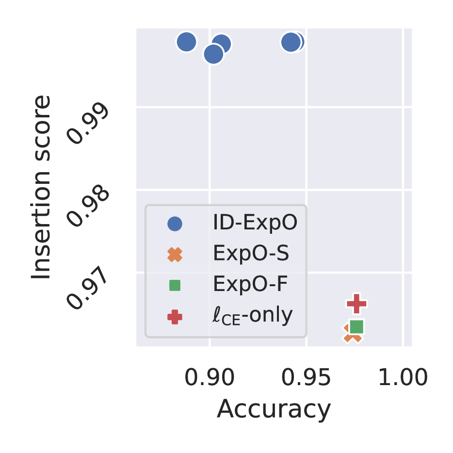
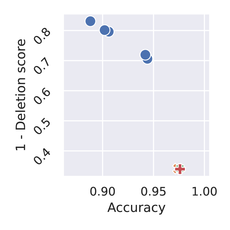
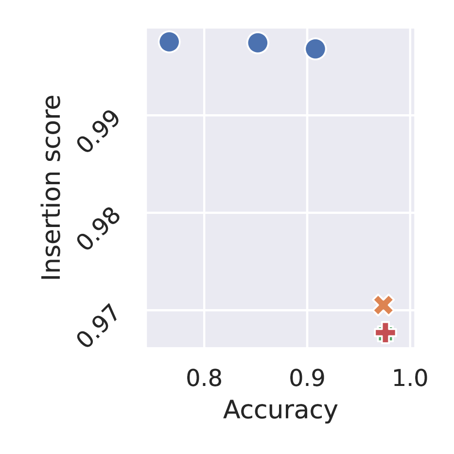
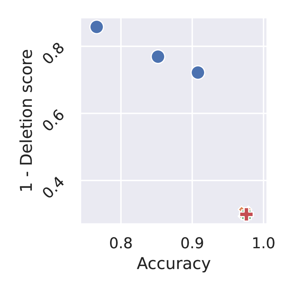
(B) LIME and KernelSHAP on collins ($S=0.5\cdot Q$)

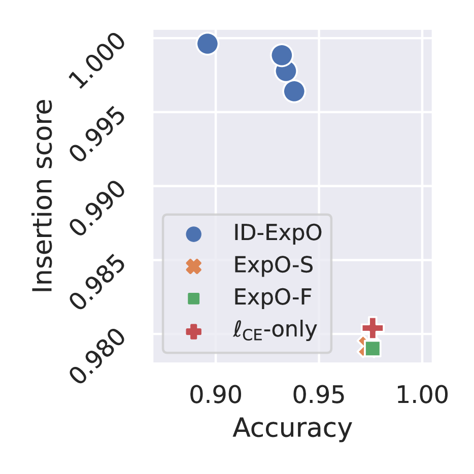
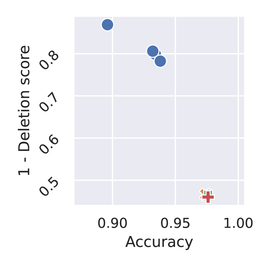
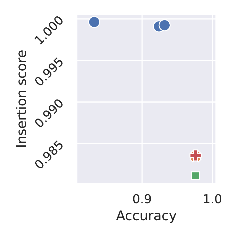
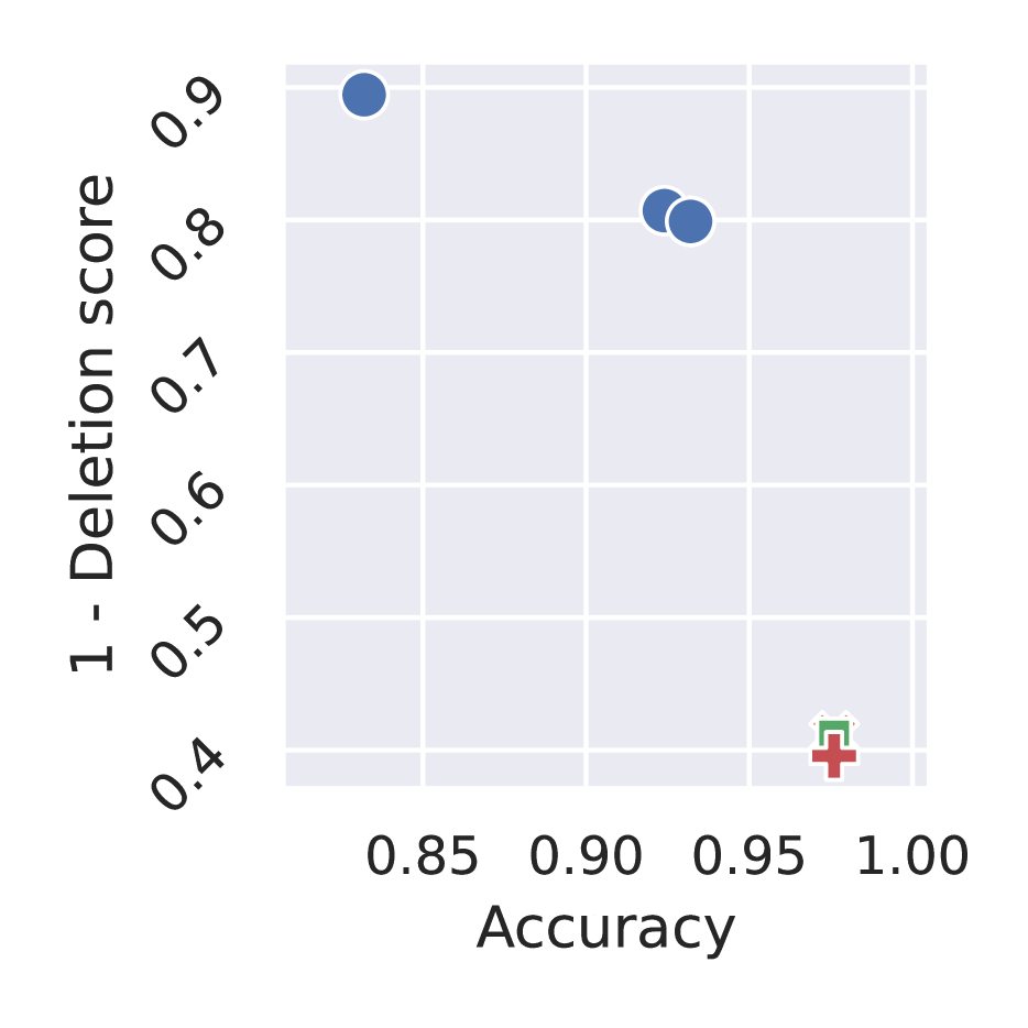
(C) LIME and KernelSHAP on mfeat-fourier ($S=0.3\cdot Q$)

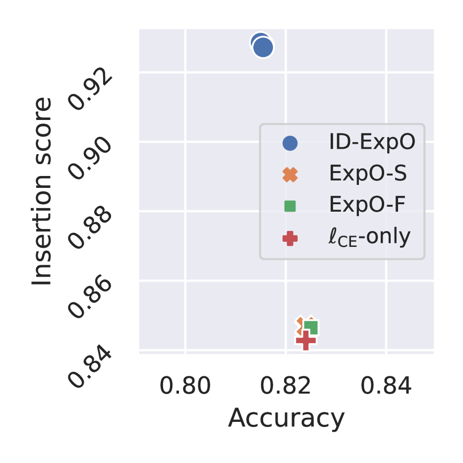
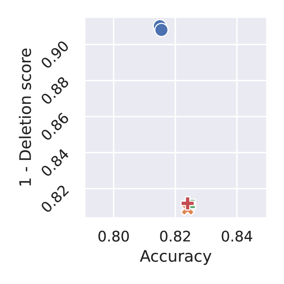
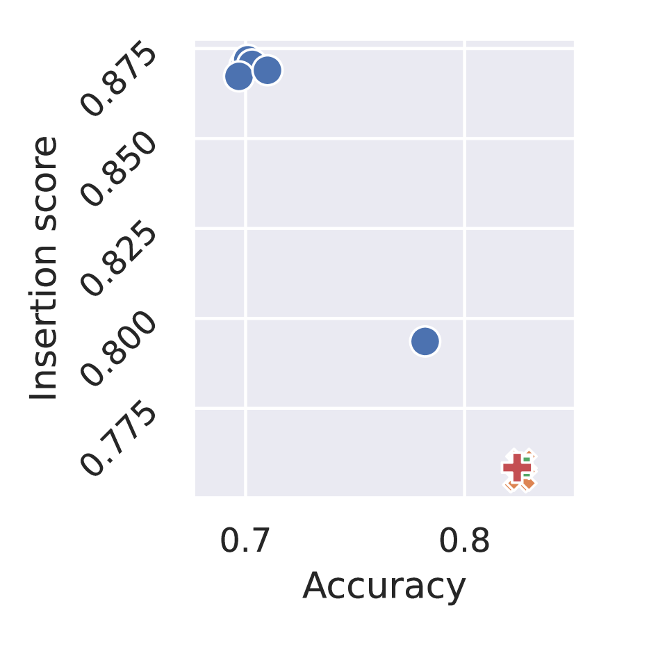
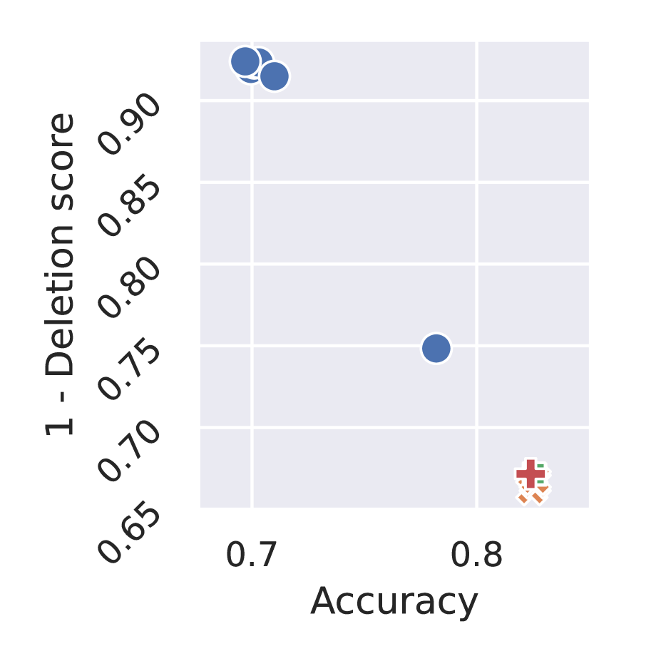
(D) LIME and KernelSHAP on mfeat-fourier ($S=0.5\cdot Q$)

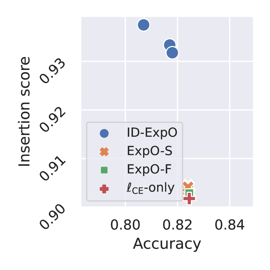
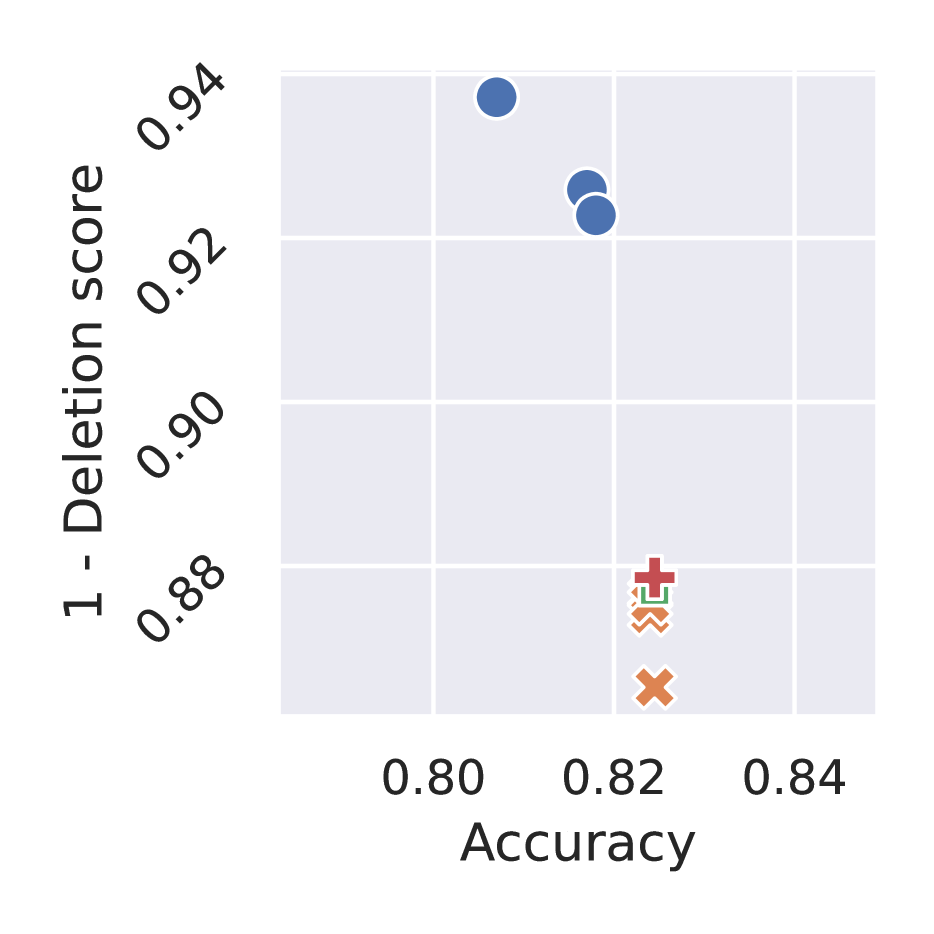
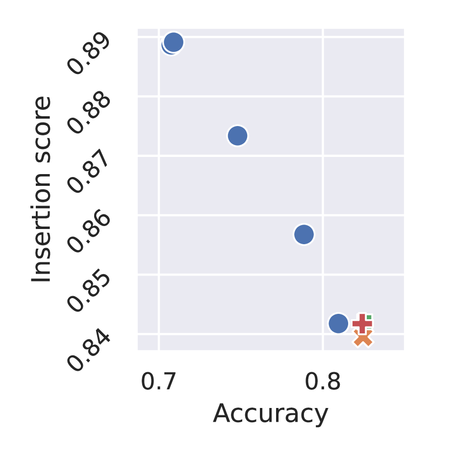
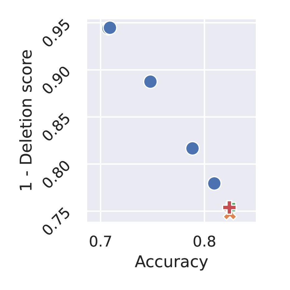
Figure A.7: Mean insertion and mean one-minus-deletion scores against accuracy on collins and mfeat-fourier datasets. The scores are averaged over the five training/validation/test sets. The first two columns show the results on LIME, while the others show the results on KernelSHAP. Each point has a different accuracy weight $\eta\in\{0.5,1.0.\cdots,3.0\}$. Higher those scores, the better.

(A) LIME and KernelSHAP on one-hundred-plants-shape ($S=0.3\cdot Q$)

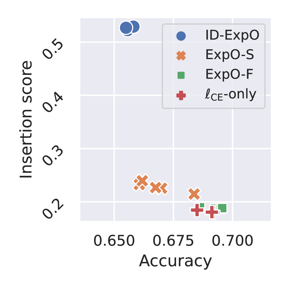
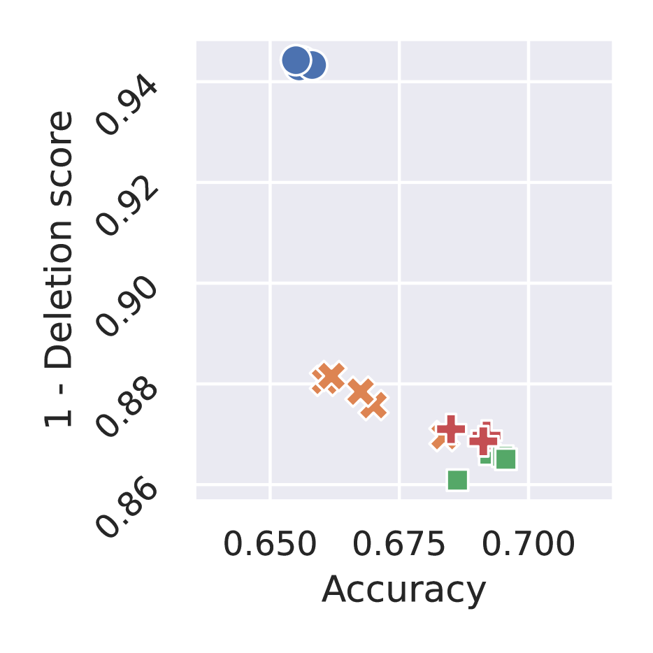
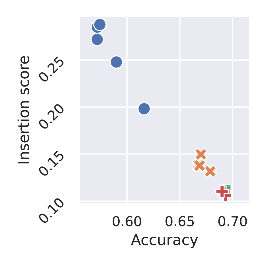
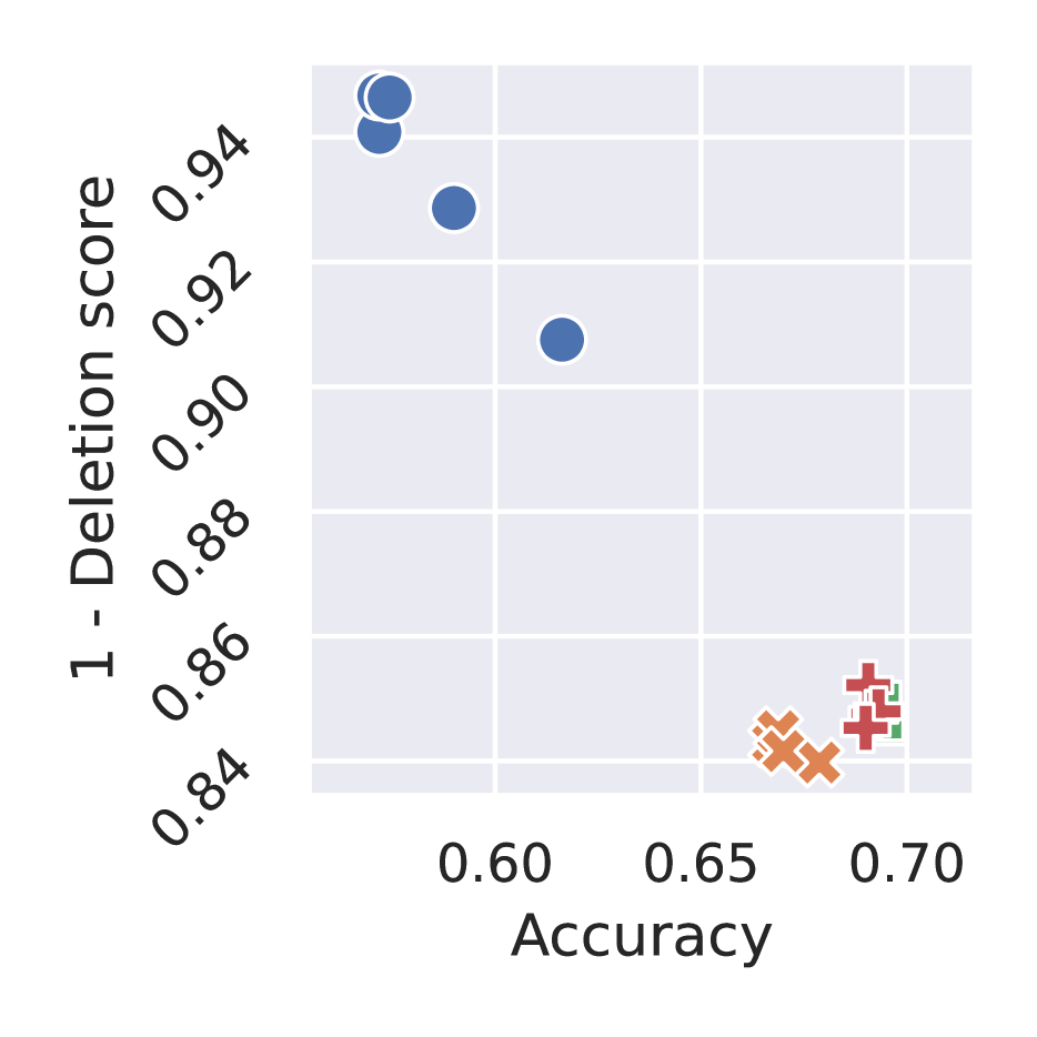
(B) LIME and KernelSHAP on one-hundred-plants-shape ($S=0.5\cdot Q$)

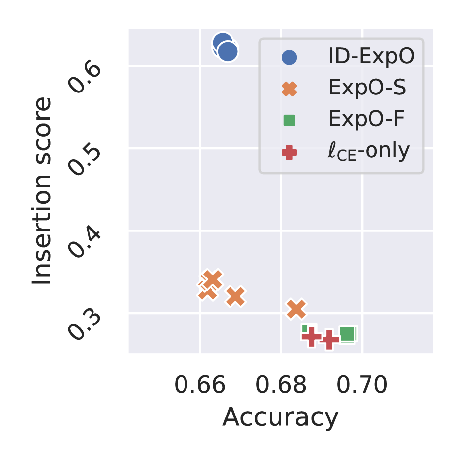
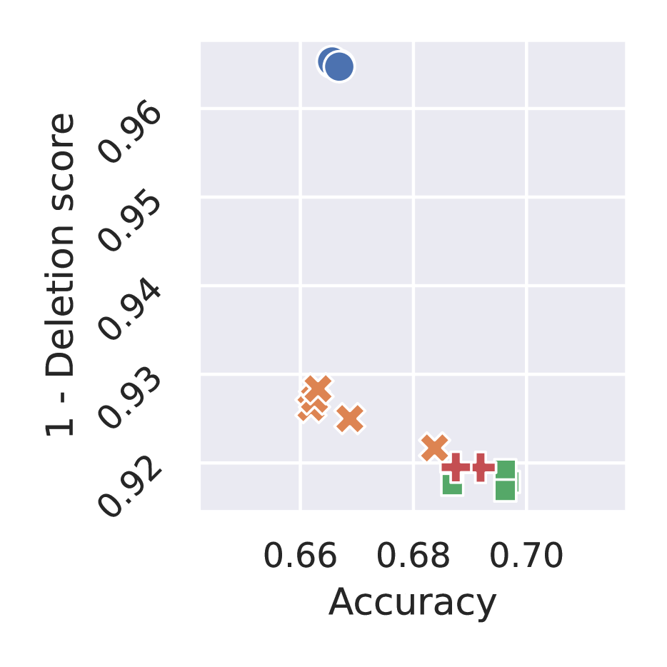
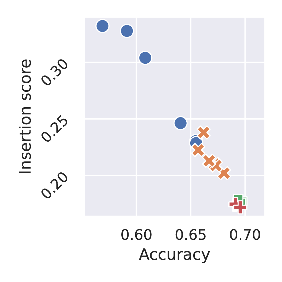
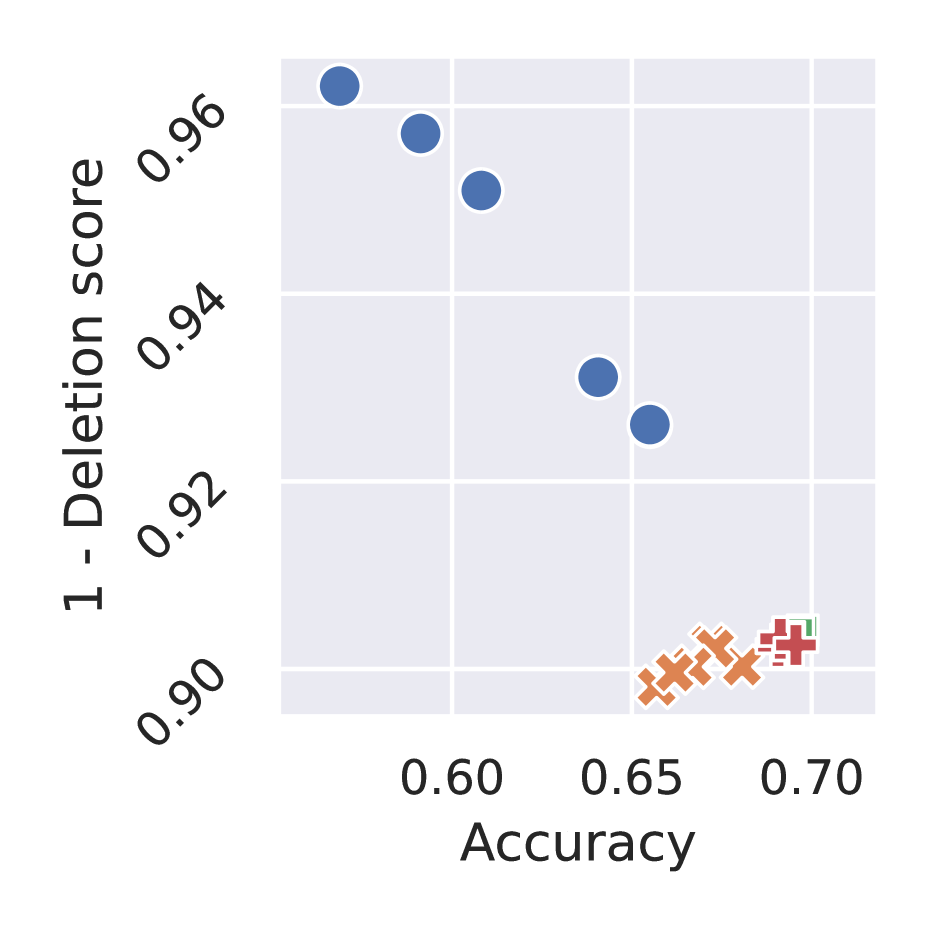
(C) LIME and KernelSHAP on qsar-biodeg ($S=0.3\cdot Q$)

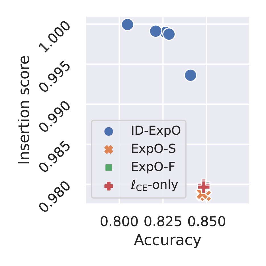
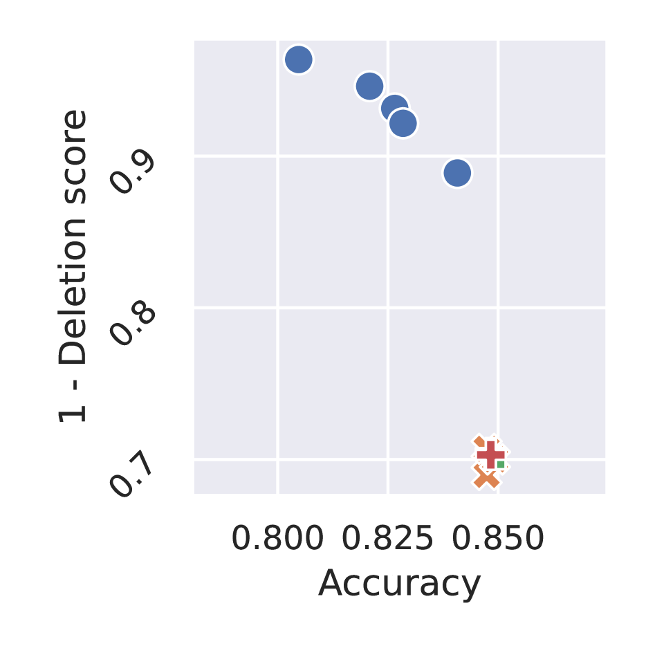
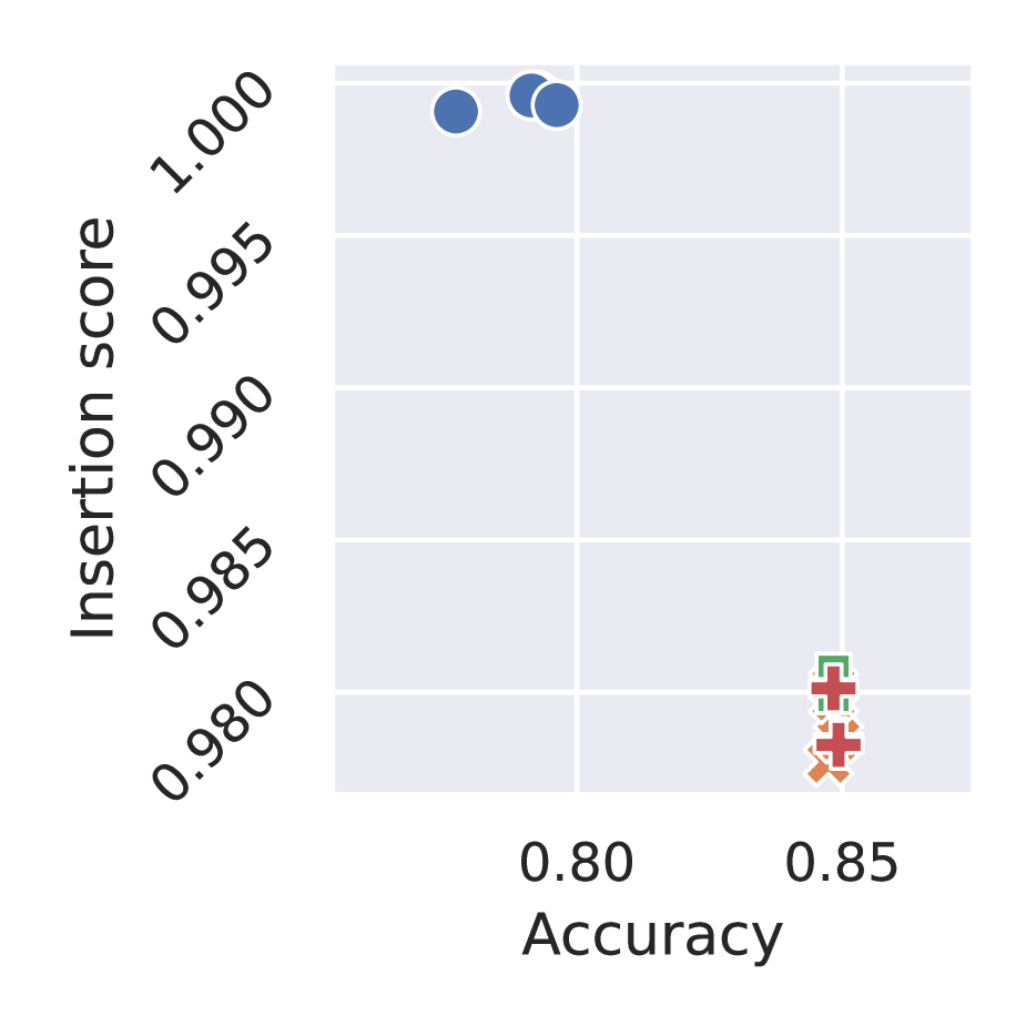
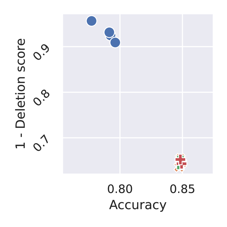
(D) LIME and KernelSHAP on qsar-biodeg ($S=0.5\cdot Q$)

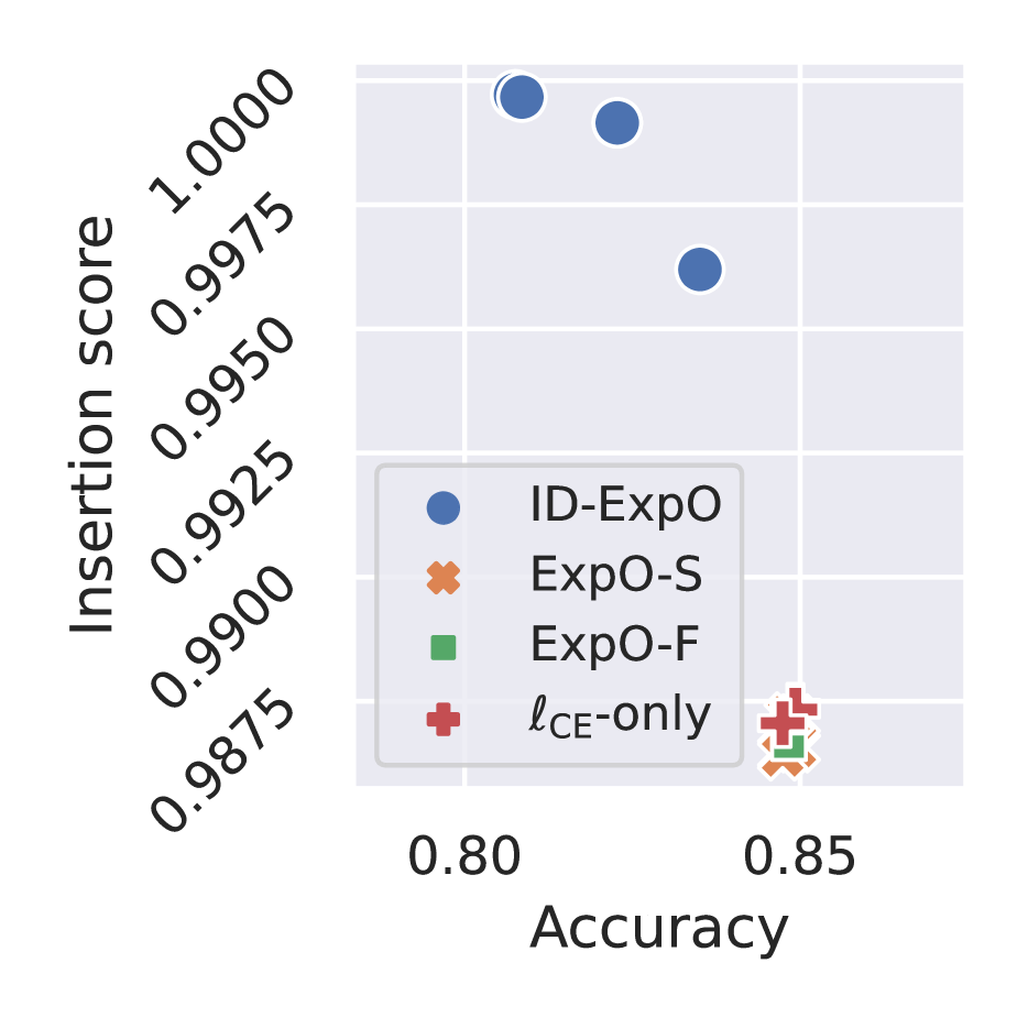
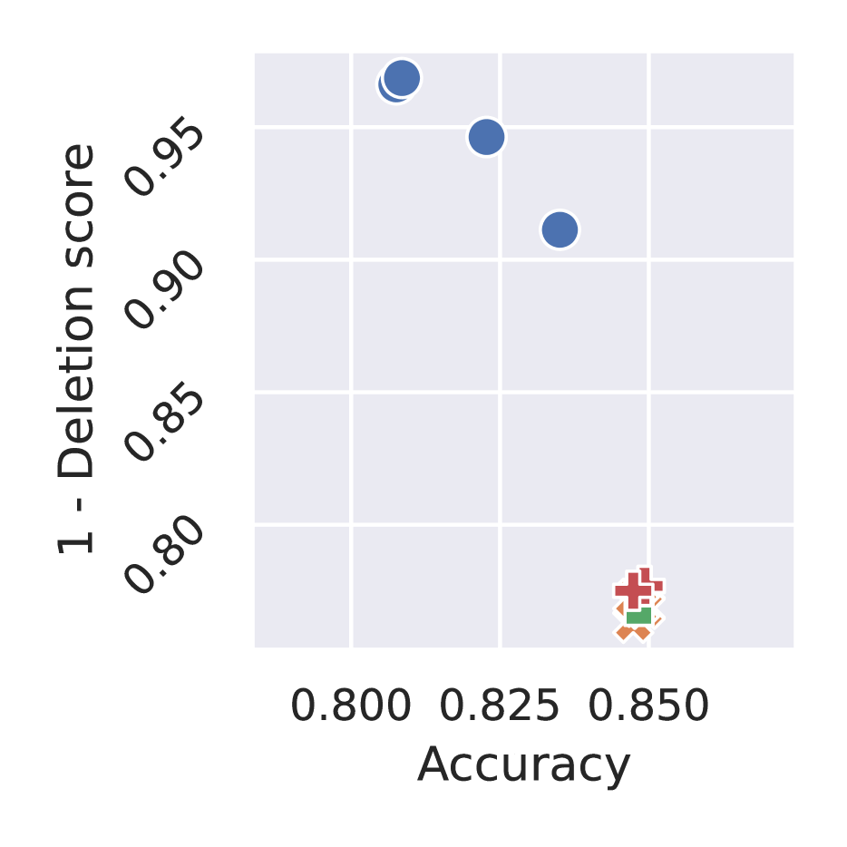
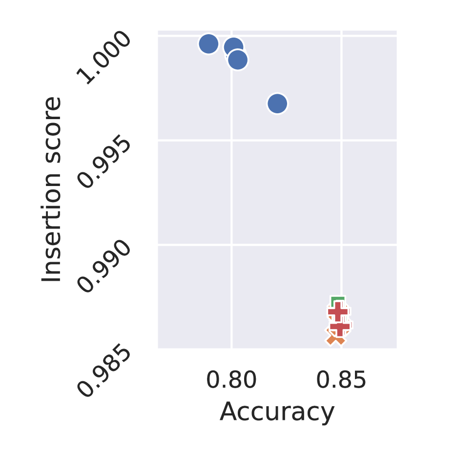
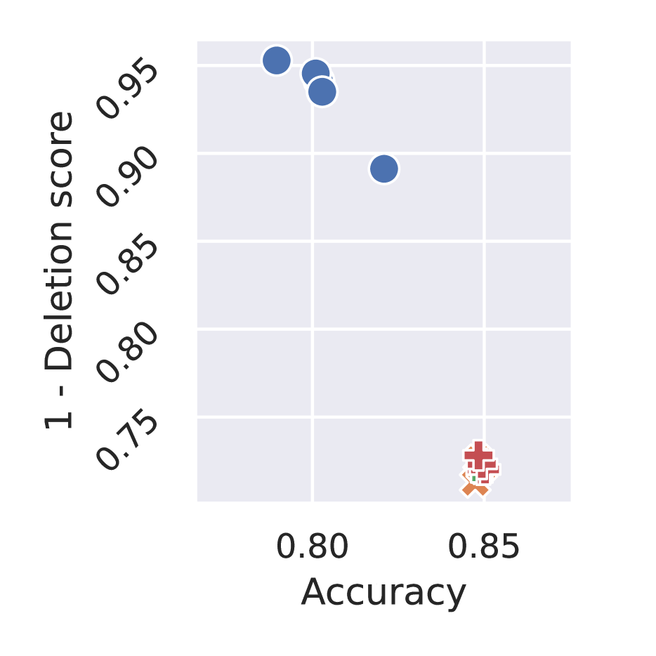
Figure A.8: Mean insertion and mean one-minus-deletion scores against accuracy on one-hundred-plants-shape and qsar-biodeg datasets. How to read these figures is the same as Figure A.7.

(A) LIME and KernelSHAP on steel-plates-fault ($S=0.3\cdot Q$)

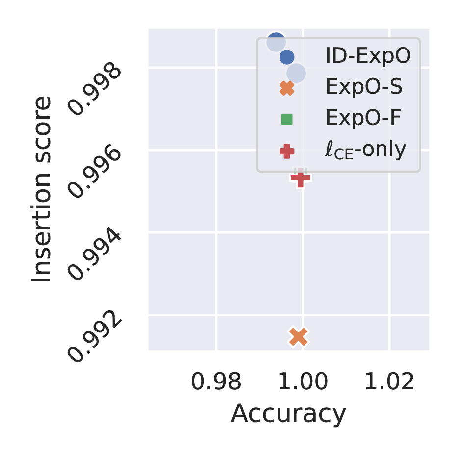
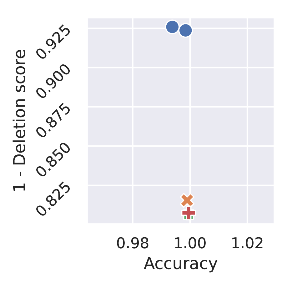
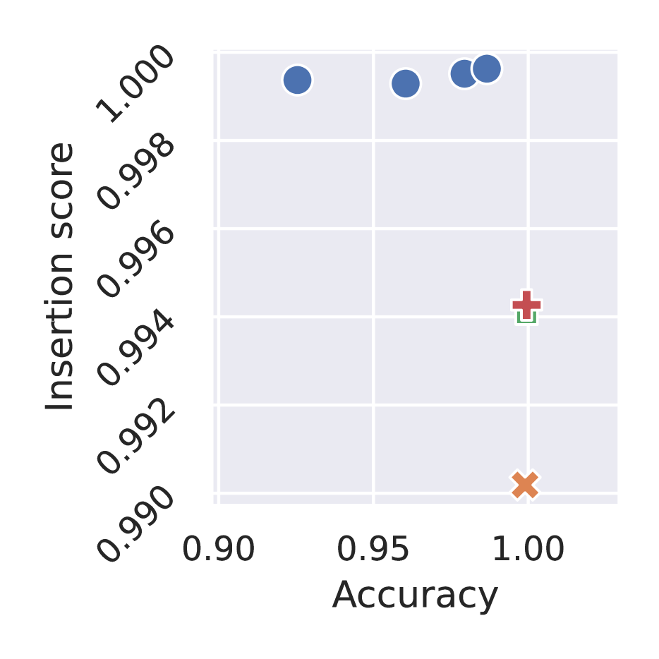
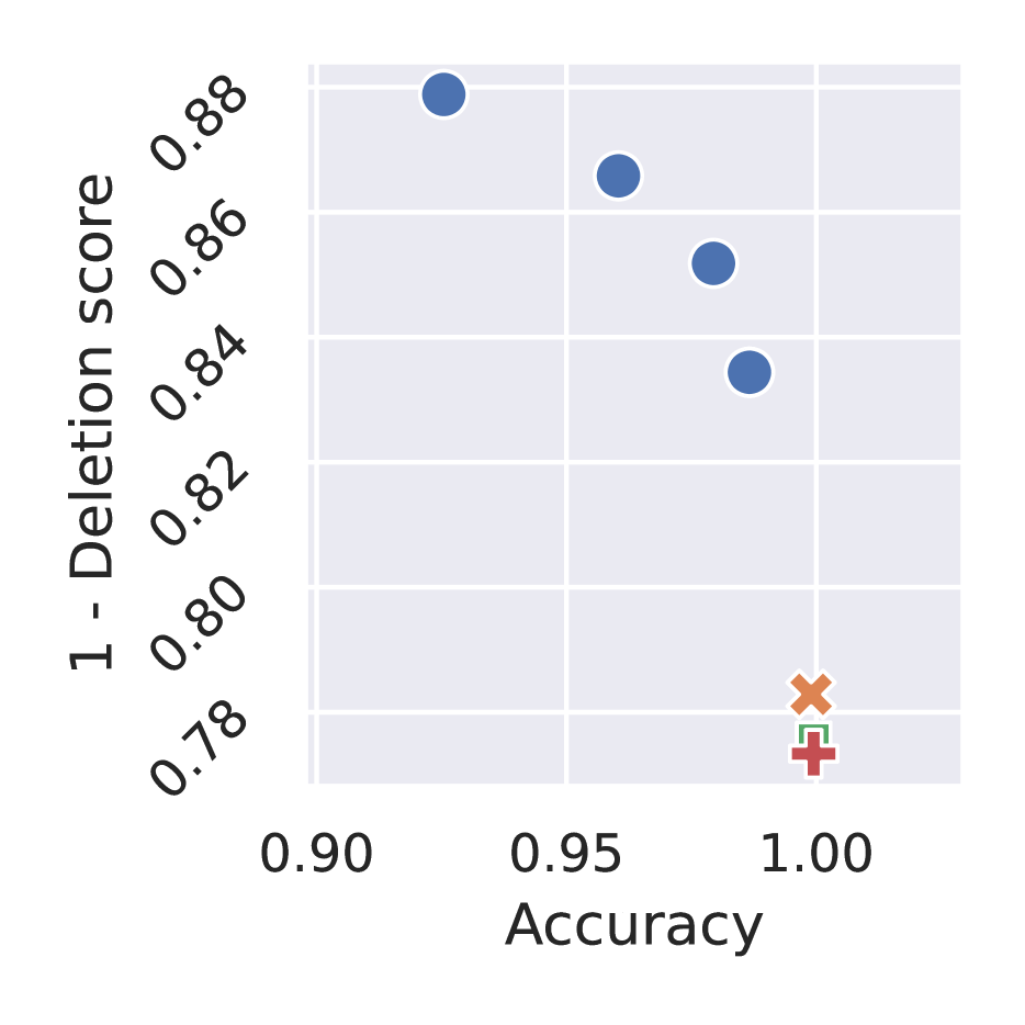
(B) LIME and KernelSHAP on steel-plates-fault ($S=0.5\cdot Q$)

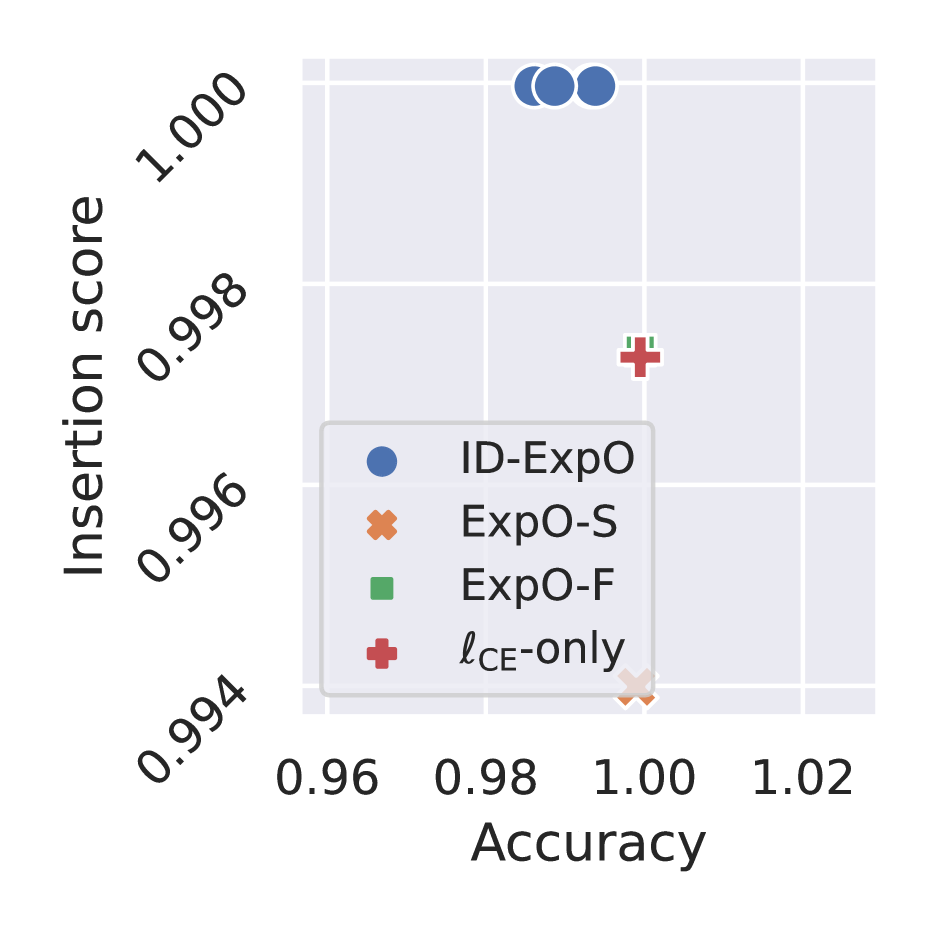
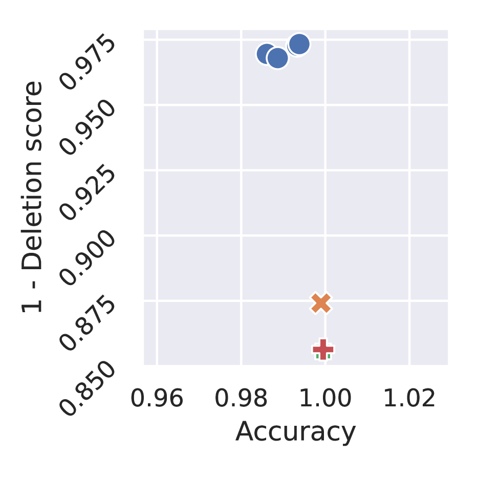
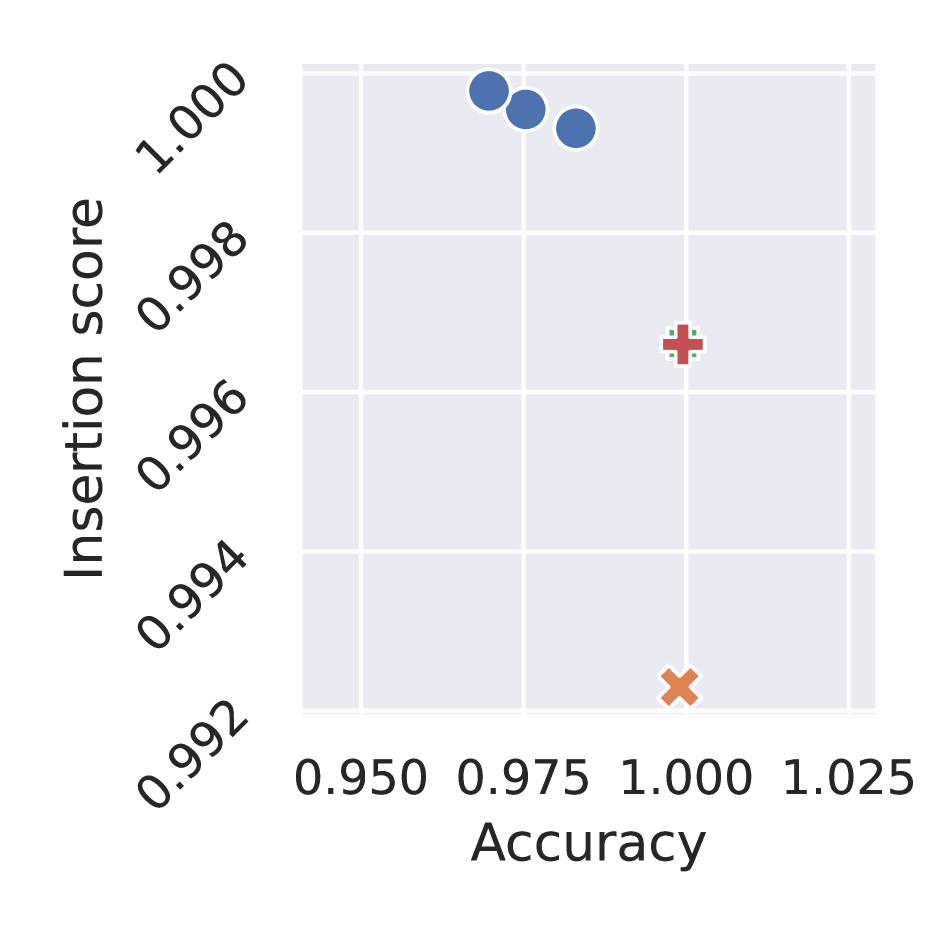
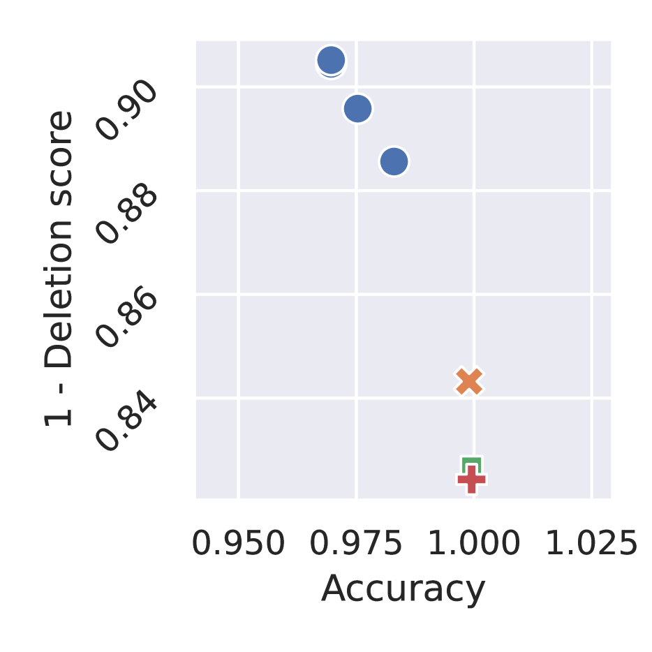
(C) LIME and KernelSHAP on wine-quality-red ($S=0.3\cdot Q$)

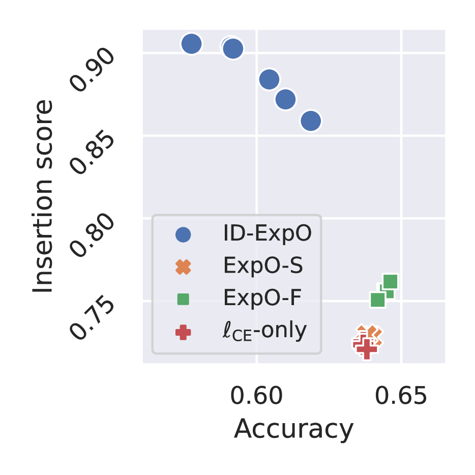
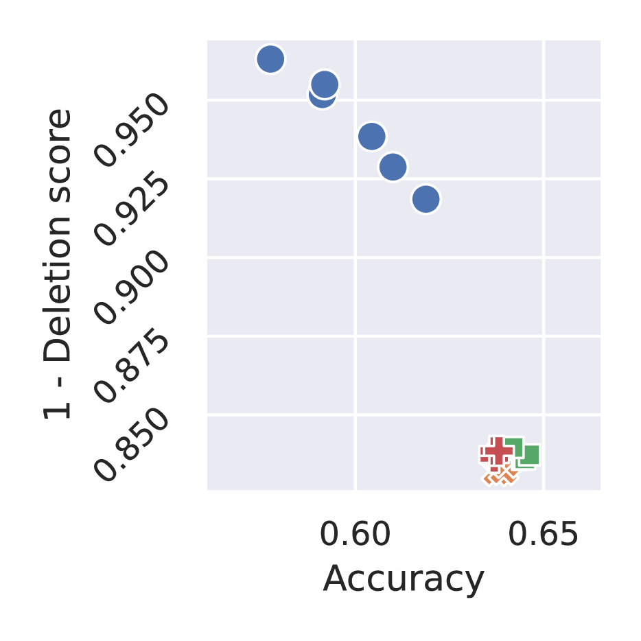
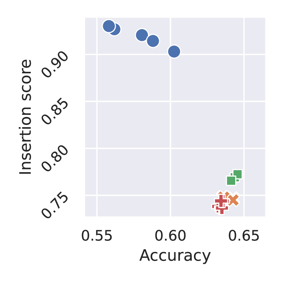
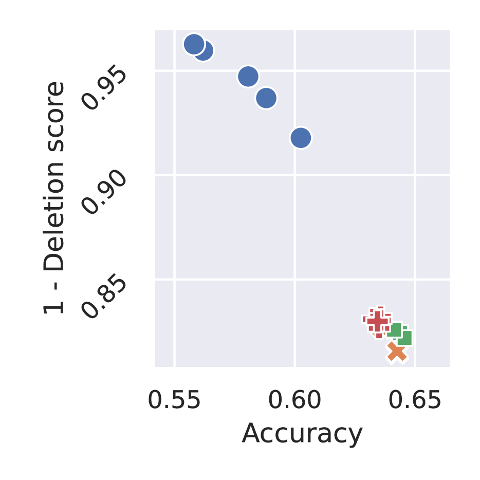
(D) LIME and KernelSHAP on wine-quality-red ($S=0.5\cdot Q$)

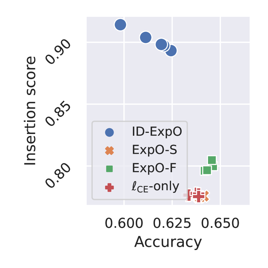
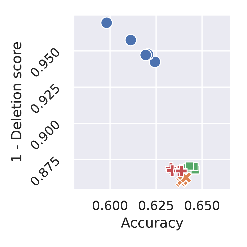
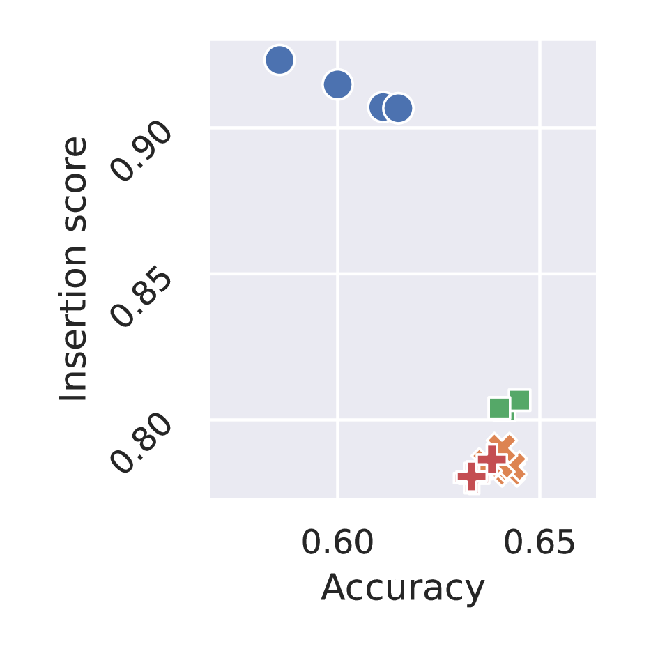
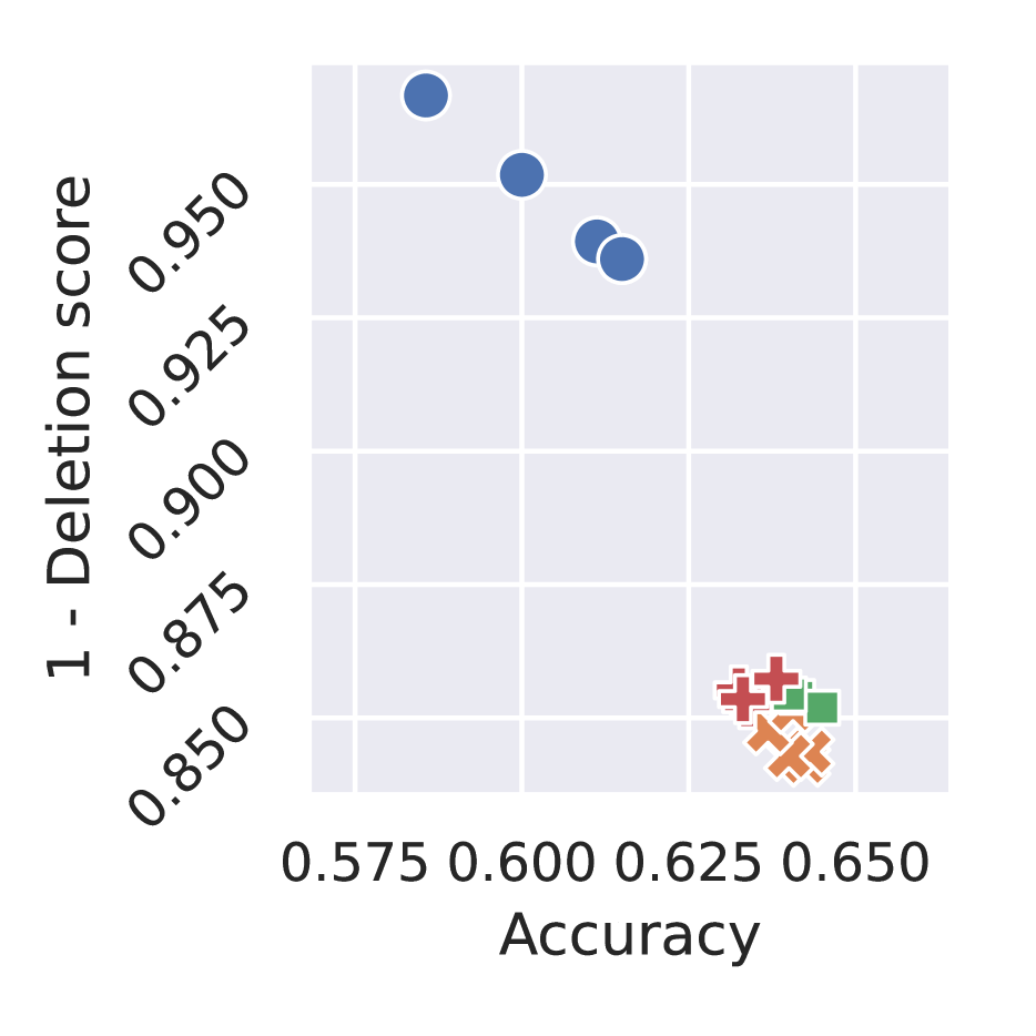
Figure A.9: Mean insertion and mean one-minus-deletion scores against accuracy on steel-plates-fault and wine-quality-red datasets. How to read these figures is the same as Figure A.7.

Appendix D Broader Impact

The proposed method can contribute to producing faithful explanations that capture the predictor’s behaviors well. However, the fact does not guarantee that the explanations are easy-to-understand for humans. If the predictor and explainer that are trained using the proposed method produce explanations that are faithful but difficult to understand for humans, they might give users wrong interpretations of the prediction results. There are several studies that explore producing explanations that are easy to understand for humans, which include human-in-the-loop approaches [89, 90] and using ground truths of explanations by human annotators [91, 92]. By using the proposed method together with such approaches, we can alleviate the concern of such misinterpretation while keeping high faithfulness in the explanations.

Appendix E Limitations

The proposed method can contribute to producing faithful explanations that capture the predictor’s behaviors well. However, the fact does not guarantee that the explanations are easy-to-understand for humans. There are several studies that explore producing explanations that are easy to understand for humans, which include human-in-the-loop approaches [89, 90] and using the ground truth of explanations by human annotators [91, 92]. When we require easy-to-understand explanations, combining the proposed method with such approaches would result in producing faithful and easy-to-understand explanations.

The proposed method is applicable to a wide range of predictors and explainers. In practice, the computational complexities of the predictor and explainer we use can be barriers to using the proposed method. The perturbation-based explainers, such as LIME and KernelSHAP, produce an explanation for an input sample by using $M$ perturbed samples around the input sample. In our experiment, $M$ was set to 200, and the mini-batch size was 128. This means that $200\times 128=25,600$ samples were used to update the predictor’s parameters $\theta$ once. For this issue, fast computation is possible by performing the data parallel training using multiple GPUs. On the other hand, using Grad-CAM, one of the gradient-based explainers, as an explainer in the proposed method is computationally more efficient than LIME and KernelSHAP because it does not need to increase the sample. Note that, although those computational complexities affect training efficiency using the proposed method, the computational complexities of the predictor and explainer in testing are invariant before and after applying the proposed method.

References

- [1] Andreas Holzinger, Chris Biemann, Constantinos S Pattichis and Douglas B Kell “What do we need to build explainable AI systems for the medical domain?”, 2017 arXiv: http://arxiv.org/abs/1712.09923
- [2] Daniel Omeiza, Helena Webb, Marina Jirotka and Lars Kunze “Explanations in Autonomous Driving: A Survey” In IEEE Transactions on Intelligent Transportation Systems 23.8, 2022, pp. 10142–10162 DOI: 10.1109/TITS.2021.3122865
- [3] Nicola Capuano, Giuseppe Fenza, Vincenzo Loia and Claudio Stanzione “Explainable Artificial Intelligence in CyberSecurity: A Survey” In IEEE Access 10, 2022, pp. 93575–93600 DOI: 10.1109/ACCESS.2022.3204171
- [4] Yongfeng Zhang and Xu Chen “Explainable Recommendation: A Survey and New Perspectives” In Found. Trends Inf. Retr. 14.1 Hanover, MA, USA: Now Publishers Inc., 2020, pp. 1–101 DOI: 10.1561/1500000066
- [5] Bas Stein, Diederick Vermetten, Fabio Caraffini and Anna V Kononova “Deep-BIAS: Detecting Structural Bias using Explainable AI”, 2023 arXiv: http://arxiv.org/abs/2304.01869
- [6] Piyawat Lertvittayakumjorn and Francesca Toni “Explanation-Based Human Debugging of NLP Models: A Survey” In Transactions of the Association for Computational Linguistics 9 Cambridge, MA: MIT Press, 2021, pp. 1508–1528 DOI: 10.1162/tacl_a_00440
- [7] Marco Tulio Ribeiro, Sameer Singh and Carlos Guestrin “" Why should i trust you?" Explaining the predictions of any classifier” In Proceedings of the 22nd ACM SIGKDD international conference on knowledge discovery and data mining, 2016, pp. 1135–1144
- [8] Scott M Lundberg and Su-In Lee “A Unified Approach to Interpreting Model Predictions” In Advances in Neural Information Processing Systems 30 Curran Associates, Inc., 2017, pp. 4765–4774 URL: http://papers.nips.cc/paper/7062-a-unified-approach-to-interpreting-model-predictions.pdf
- [9] Ramprasaath R Selvaraju et al. “Grad-CAM: Visual Explanations from Deep Networks via Gradient-Based Localization” In International journal of computer vision 128.2, 2020, pp. 336–359 DOI: 10.1007/s11263-019-01228-7
- [10] Trevor Hastie and Robert Tibshirani “Generalized Additive Models” In Statistical Science 1.3 Institute of Mathematical Statistics, 1986, pp. 297–310 URL: http://www.jstor.org/stable/2245459
- [11] David Alvarez Melis and Tommi Jaakkola “Towards robust interpretability with self-explaining neural networks” In Advances in neural information processing systems 31, 2018
- [12] Vitali Petsiuk, Abir Das and Kate Saenko “RISE: Randomized Input Sampling for Explanation of Black-box Models”, 2018 arXiv:1806.07421 [cs.CV]
- [13] Arne Gevaert et al. “Evaluating Feature Attribution Methods in the Image Domain” In ArXiv, 2022 URL: https://www.semanticscholar.org/paper/65f8cf77942dd5067ba96debc90aa009467c990d
- [14] Gregory Plumb et al. “Regularizing black-box models for improved interpretability” In Advances in Neural Information Processing Systems 33, 2020, pp. 10526–10536
- [15] Aditya Chattopadhay, Anirban Sarkar, Prantik Howlader and Vineeth N Balasubramanian “Grad-cam++: Generalized gradient-based visual explanations for deep convolutional networks” In 2018 IEEE winter conference on applications of computer vision (WACV), 2018, pp. 839–847 IEEE
- [16] Ruigang Fu et al. “Axiom-based grad-cam: Towards accurate visualization and explanation of cnns” In arXiv preprint arXiv:2008.02312, 2020
- [17] Peng-Tao Jiang et al. “Layercam: Exploring hierarchical class activation maps for localization” In IEEE Transactions on Image Processing 30 IEEE, 2021, pp. 5875–5888
- [18] Xingyu Zhao et al. “Baylime: Bayesian local interpretable model-agnostic explanations” In Uncertainty in artificial intelligence, 2021, pp. 887–896 PMLR
- [19] Haofan Wang et al. “Score-CAM: Score-weighted visual explanations for convolutional neural networks” In Proceedings of the IEEE/CVF conference on computer vision and pattern recognition workshops, 2020, pp. 24–25
- [20] Ruth Fong, Mandela Patrick and Andrea Vedaldi “Understanding deep networks via extremal perturbations and smooth masks” In Proceedings of the IEEE/CVF international conference on computer vision, 2019, pp. 2950–2958
- [21] Hanwei Zhang et al. “Opti-CAM: Optimizing saliency maps for interpretability”, 2023 arXiv: http://arxiv.org/abs/2301.07002
- [22] Christoph Molnar “Interpretable Machine Learning”, 2022 URL: https://christophm.github.io/interpretable-ml-book
- [23] Rishabh Agarwal et al. “Neural additive models: Interpretable machine learning with neural nets” In Advances in Neural Information Processing Systems 34, 2021, pp. 4699–4711
- [24] Patrick Schwab, Djordje Miladinovic and Walter Karlen “Granger-Causal Attentive Mixtures of Experts: Learning Important Features with Neural Networks” In AAAI Conference on Artificial Intelligence, 2018
- [25] Hiroshi Fukui, Tsubasa Hirakawa, Takayoshi Yamashita and Hironobu Fujiyoshi “Attention branch network: Learning of attention mechanism for visual explanation” In Proceedings of the IEEE/CVF conference on computer vision and pattern recognition, 2019, pp. 10705–10714
- [26] Tsumugi Iida et al. “Visual Explanation Generation Based on Lambda Attention Branch Networks” In Proceedings of the Asian Conference on Computer Vision (ACCV), 2022, pp. 3536–3551
- [27] Jianlong Zhou, Amir H Gandomi, Fang Chen and Andreas Holzinger “Evaluating the Quality of Machine Learning Explanations: A Survey on Methods and Metrics” In Electronics 10.5 Multidisciplinary Digital Publishing Institute, 2021, pp. 593 DOI: 10.3390/electronics10050593
- [28] Marco Ancona, Enea Ceolini, Cengiz Öztireli and Markus Gross “Towards better understanding of gradient-based attribution methods for Deep Neural Networks”, 2018 URL: https://openreview.net/pdf?id=Sy21R9JAW
- [29] Harish Guruprasad Ramaswamy “Ablation-cam: Visual explanations for deep convolutional network via gradient-free localization” In Proceedings of the IEEE/CVF Winter Conference on Applications of Computer Vision, 2020, pp. 983–991
- [30] Laura Rieger and Lars Kai Hansen “Irof: a low resource evaluation metric for explanation methods” In arXiv preprint arXiv:2003.08747, 2020
- [31] Amirata Ghorbani, Abubakar Abid and James Zou “Interpretation of neural networks is fragile” In Proceedings of the AAAI conference on artificial intelligence 33.01, 2019, pp. 3681–3688
- [32] Umang Bhatt, Adrian Weller and José MF Moura “Evaluating and aggregating feature-based model explanations” In Proceedings of the Twenty-Ninth International Conference on International Joint Conferences on Artificial Intelligence, 2021, pp. 3016–3022
- [33] Aya Abdelsalam Ismail, Hector Corrada Bravo and Soheil Feizi “Improving deep learning interpretability by saliency guided training” In Advances in neural information processing systems 34 proceedings.neurips.cc, 2021, pp. 26726–26739 URL: https://proceedings.neurips.cc/paper/2021/hash/e0cd3f16f9e883ca91c2a4c24f47b3d9-Abstract.html
- [34] Qinglong Zhang, Lu Rao and Yubin Yang “Group-cam: Group score-weighted visual explanations for deep convolutional networks” In arXiv preprint arXiv:2103.13859, 2021
- [35] Marco Huber, Meiling Fang, Fadi Boutros and Naser Damer “Are Explainability Tools Gender Biased? A Case Study on Face Presentation Attack Detection” In arXiv preprint arXiv:2304.13419, 2023
- [36] Chunyan Zeng et al. “Abs-CAM: a gradient optimization interpretable approach for explanation of convolutional neural networks” In Signal, Image and Video Processing Springer, 2022, pp. 1–8
- [37] Saachi Jain et al. “Missingness Bias in Model Debugging”, 2022 arXiv: http://arxiv.org/abs/2204.08945
- [38] Alex Krizhevsky and Geoffrey Hinton “Learning multiple layers of features from tiny images” Toronto, ON, Canada, 2009
- [39] Adam Coates, Andrew Ng and Honglak Lee “An Analysis of Single-Layer Networks in Unsupervised Feature Learning” In Proceedings of the Fourteenth International Conference on Artificial Intelligence and Statistics 15, Proceedings of Machine Learning Research Fort Lauderdale, FL, USA: PMLR, 2011, pp. 215–223 URL: https://proceedings.mlr.press/v15/coates11a.html
- [40] Kaiming He, Xiangyu Zhang, Shaoqing Ren and Jian Sun “Deep residual learning for image recognition” In Proceedings of the IEEE conference on computer vision and pattern recognition, 2016, pp. 770–778
- [41] Xuelin Situ et al. “Learning to Explain: Generating Stable Explanations Fast” In Proceedings of the 59th Annual Meeting of the Association for Computational Linguistics and the 11th International Joint Conference on Natural Language Processing (Volume 1: Long Papers) Online: Association for Computational Linguistics, 2021, pp. 5340–5355 DOI: 10.18653/v1/2021.acl-long.415
- [42] Bernd Bischl et al. “OpenML Benchmarking Suites.” In Proceedings of the NeurIPS 2021 Datasets and Benchmarks Track, 2021
- [43] Isaac Lage et al. “Human-in-the-Loop Interpretability Prior” In Advances in neural information processing systems 31, 2018 URL: https://www.ncbi.nlm.nih.gov/pubmed/33623354
- [44] Yuyang Gao, Tong Steven Sun, Liang Zhao and Sungsoo Ray Hong “Aligning eyes between humans and deep neural network through interactive attention alignment” In Proceedings of the ACM on Human-Computer Interaction 6.CSCW2 ACM New York, NY, USA, 2022, pp. 1–28
- [45] Andrew Slavin Ross, Michael C Hughes and Finale Doshi-Velez “Right for the right reasons: training differentiable models by constraining their explanations” In Proceedings of the 26th International Joint Conference on Artificial Intelligence, 2017, pp. 2662–2670
- [46] Vladimir Balayan et al. “Teaching the Machine to Explain Itself using Domain Knowledge” In arXiv preprint arXiv:2012.01932, 2020

References

- [47] Andreas Holzinger, Chris Biemann, Constantinos S Pattichis and Douglas B Kell “What do we need to build explainable AI systems for the medical domain?”, 2017 arXiv: http://arxiv.org/abs/1712.09923
- [48] Daniel Omeiza, Helena Webb, Marina Jirotka and Lars Kunze “Explanations in Autonomous Driving: A Survey” In IEEE Transactions on Intelligent Transportation Systems 23.8, 2022, pp. 10142–10162 DOI: 10.1109/TITS.2021.3122865
- [49] Nicola Capuano, Giuseppe Fenza, Vincenzo Loia and Claudio Stanzione “Explainable Artificial Intelligence in CyberSecurity: A Survey” In IEEE Access 10, 2022, pp. 93575–93600 DOI: 10.1109/ACCESS.2022.3204171
- [50] Yongfeng Zhang and Xu Chen “Explainable Recommendation: A Survey and New Perspectives” In Found. Trends Inf. Retr. 14.1 Hanover, MA, USA: Now Publishers Inc., 2020, pp. 1–101 DOI: 10.1561/1500000066
- [51] Bas Stein, Diederick Vermetten, Fabio Caraffini and Anna V Kononova “Deep-BIAS: Detecting Structural Bias using Explainable AI”, 2023 arXiv: http://arxiv.org/abs/2304.01869
- [52] Piyawat Lertvittayakumjorn and Francesca Toni “Explanation-Based Human Debugging of NLP Models: A Survey” In Transactions of the Association for Computational Linguistics 9 Cambridge, MA: MIT Press, 2021, pp. 1508–1528 DOI: 10.1162/tacl_a_00440
- [53] Marco Tulio Ribeiro, Sameer Singh and Carlos Guestrin “" Why should i trust you?" Explaining the predictions of any classifier” In Proceedings of the 22nd ACM SIGKDD international conference on knowledge discovery and data mining, 2016, pp. 1135–1144
- [54] Scott M Lundberg and Su-In Lee “A Unified Approach to Interpreting Model Predictions” In Advances in Neural Information Processing Systems 30 Curran Associates, Inc., 2017, pp. 4765–4774 URL: http://papers.nips.cc/paper/7062-a-unified-approach-to-interpreting-model-predictions.pdf
- [55] Ramprasaath R Selvaraju et al. “Grad-CAM: Visual Explanations from Deep Networks via Gradient-Based Localization” In International journal of computer vision 128.2, 2020, pp. 336–359 DOI: 10.1007/s11263-019-01228-7
- [56] Trevor Hastie and Robert Tibshirani “Generalized Additive Models” In Statistical Science 1.3 Institute of Mathematical Statistics, 1986, pp. 297–310 URL: http://www.jstor.org/stable/2245459
- [57] David Alvarez Melis and Tommi Jaakkola “Towards robust interpretability with self-explaining neural networks” In Advances in neural information processing systems 31, 2018
- [58] Vitali Petsiuk, Abir Das and Kate Saenko “RISE: Randomized Input Sampling for Explanation of Black-box Models”, 2018 arXiv:1806.07421 [cs.CV]
- [59] Arne Gevaert et al. “Evaluating Feature Attribution Methods in the Image Domain” In ArXiv, 2022 URL: https://www.semanticscholar.org/paper/65f8cf77942dd5067ba96debc90aa009467c990d
- [60] Gregory Plumb et al. “Regularizing black-box models for improved interpretability” In Advances in Neural Information Processing Systems 33, 2020, pp. 10526–10536
- [61] Aditya Chattopadhay, Anirban Sarkar, Prantik Howlader and Vineeth N Balasubramanian “Grad-cam++: Generalized gradient-based visual explanations for deep convolutional networks” In 2018 IEEE winter conference on applications of computer vision (WACV), 2018, pp. 839–847 IEEE
- [62] Ruigang Fu et al. “Axiom-based grad-cam: Towards accurate visualization and explanation of cnns” In arXiv preprint arXiv:2008.02312, 2020
- [63] Peng-Tao Jiang et al. “Layercam: Exploring hierarchical class activation maps for localization” In IEEE Transactions on Image Processing 30 IEEE, 2021, pp. 5875–5888
- [64] Xingyu Zhao et al. “Baylime: Bayesian local interpretable model-agnostic explanations” In Uncertainty in artificial intelligence, 2021, pp. 887–896 PMLR
- [65] Haofan Wang et al. “Score-CAM: Score-weighted visual explanations for convolutional neural networks” In Proceedings of the IEEE/CVF conference on computer vision and pattern recognition workshops, 2020, pp. 24–25
- [66] Ruth Fong, Mandela Patrick and Andrea Vedaldi “Understanding deep networks via extremal perturbations and smooth masks” In Proceedings of the IEEE/CVF international conference on computer vision, 2019, pp. 2950–2958
- [67] Hanwei Zhang et al. “Opti-CAM: Optimizing saliency maps for interpretability”, 2023 arXiv: http://arxiv.org/abs/2301.07002
- [68] Christoph Molnar “Interpretable Machine Learning”, 2022 URL: https://christophm.github.io/interpretable-ml-book
- [69] Rishabh Agarwal et al. “Neural additive models: Interpretable machine learning with neural nets” In Advances in Neural Information Processing Systems 34, 2021, pp. 4699–4711
- [70] Patrick Schwab, Djordje Miladinovic and Walter Karlen “Granger-Causal Attentive Mixtures of Experts: Learning Important Features with Neural Networks” In AAAI Conference on Artificial Intelligence, 2018
- [71] Hiroshi Fukui, Tsubasa Hirakawa, Takayoshi Yamashita and Hironobu Fujiyoshi “Attention branch network: Learning of attention mechanism for visual explanation” In Proceedings of the IEEE/CVF conference on computer vision and pattern recognition, 2019, pp. 10705–10714
- [72] Tsumugi Iida et al. “Visual Explanation Generation Based on Lambda Attention Branch Networks” In Proceedings of the Asian Conference on Computer Vision (ACCV), 2022, pp. 3536–3551
- [73] Jianlong Zhou, Amir H Gandomi, Fang Chen and Andreas Holzinger “Evaluating the Quality of Machine Learning Explanations: A Survey on Methods and Metrics” In Electronics 10.5 Multidisciplinary Digital Publishing Institute, 2021, pp. 593 DOI: 10.3390/electronics10050593
- [74] Marco Ancona, Enea Ceolini, Cengiz Öztireli and Markus Gross “Towards better understanding of gradient-based attribution methods for Deep Neural Networks”, 2018 URL: https://openreview.net/pdf?id=Sy21R9JAW
- [75] Harish Guruprasad Ramaswamy “Ablation-cam: Visual explanations for deep convolutional network via gradient-free localization” In Proceedings of the IEEE/CVF Winter Conference on Applications of Computer Vision, 2020, pp. 983–991
- [76] Laura Rieger and Lars Kai Hansen “Irof: a low resource evaluation metric for explanation methods” In arXiv preprint arXiv:2003.08747, 2020
- [77] Amirata Ghorbani, Abubakar Abid and James Zou “Interpretation of neural networks is fragile” In Proceedings of the AAAI conference on artificial intelligence 33.01, 2019, pp. 3681–3688
- [78] Umang Bhatt, Adrian Weller and José MF Moura “Evaluating and aggregating feature-based model explanations” In Proceedings of the Twenty-Ninth International Conference on International Joint Conferences on Artificial Intelligence, 2021, pp. 3016–3022
- [79] Aya Abdelsalam Ismail, Hector Corrada Bravo and Soheil Feizi “Improving deep learning interpretability by saliency guided training” In Advances in neural information processing systems 34 proceedings.neurips.cc, 2021, pp. 26726–26739 URL: https://proceedings.neurips.cc/paper/2021/hash/e0cd3f16f9e883ca91c2a4c24f47b3d9-Abstract.html
- [80] Qinglong Zhang, Lu Rao and Yubin Yang “Group-cam: Group score-weighted visual explanations for deep convolutional networks” In arXiv preprint arXiv:2103.13859, 2021
- [81] Marco Huber, Meiling Fang, Fadi Boutros and Naser Damer “Are Explainability Tools Gender Biased? A Case Study on Face Presentation Attack Detection” In arXiv preprint arXiv:2304.13419, 2023
- [82] Chunyan Zeng et al. “Abs-CAM: a gradient optimization interpretable approach for explanation of convolutional neural networks” In Signal, Image and Video Processing Springer, 2022, pp. 1–8
- [83] Saachi Jain et al. “Missingness Bias in Model Debugging”, 2022 arXiv: http://arxiv.org/abs/2204.08945
- [84] Alex Krizhevsky and Geoffrey Hinton “Learning multiple layers of features from tiny images” Toronto, ON, Canada, 2009
- [85] Adam Coates, Andrew Ng and Honglak Lee “An Analysis of Single-Layer Networks in Unsupervised Feature Learning” In Proceedings of the Fourteenth International Conference on Artificial Intelligence and Statistics 15, Proceedings of Machine Learning Research Fort Lauderdale, FL, USA: PMLR, 2011, pp. 215–223 URL: https://proceedings.mlr.press/v15/coates11a.html
- [86] Kaiming He, Xiangyu Zhang, Shaoqing Ren and Jian Sun “Deep residual learning for image recognition” In Proceedings of the IEEE conference on computer vision and pattern recognition, 2016, pp. 770–778
- [87] Xuelin Situ et al. “Learning to Explain: Generating Stable Explanations Fast” In Proceedings of the 59th Annual Meeting of the Association for Computational Linguistics and the 11th International Joint Conference on Natural Language Processing (Volume 1: Long Papers) Online: Association for Computational Linguistics, 2021, pp. 5340–5355 DOI: 10.18653/v1/2021.acl-long.415
- [88] Bernd Bischl et al. “OpenML Benchmarking Suites.” In Proceedings of the NeurIPS 2021 Datasets and Benchmarks Track, 2021
- [89] Isaac Lage et al. “Human-in-the-Loop Interpretability Prior” In Advances in neural information processing systems 31, 2018 URL: https://www.ncbi.nlm.nih.gov/pubmed/33623354
- [90] Yuyang Gao, Tong Steven Sun, Liang Zhao and Sungsoo Ray Hong “Aligning eyes between humans and deep neural network through interactive attention alignment” In Proceedings of the ACM on Human-Computer Interaction 6.CSCW2 ACM New York, NY, USA, 2022, pp. 1–28
- [91] Andrew Slavin Ross, Michael C Hughes and Finale Doshi-Velez “Right for the right reasons: training differentiable models by constraining their explanations” In Proceedings of the 26th International Joint Conference on Artificial Intelligence, 2017, pp. 2662–2670
- [92] Vladimir Balayan et al. “Teaching the Machine to Explain Itself using Domain Knowledge” In arXiv preprint arXiv:2012.01932, 2020