Commentary to Wan et al. (2014):
Estimating the standard deviation
from the sample size and range or quartiles

Abstract

This short note proposes two additive corrections to a pair of relations published in Wan et al. [WWLT14] in order to extend them to a ’small sample size’ condition. In particular we focus the interest on the possibility to provide an estimate to the sample standard deviation $\sigma$ when knowing only the sample size $n$, the range $[a,b]$ and/or the quartiles $Q_{1},Q_{3}$ of some data. Our results allow to explicitely compute $\sigma$, for instance with software R or any spreadsheet, for any sample size $n\geq 2$. R codes and data are publicly available on https://github.com/MassimoBorelli/sd

Mathematics Subject Classification (MSC): 62P10

1 Background

In their 2014 BMC medical research methodology paper [WWLT14], Xiang Wan and colleagues improve a previous work by Stela Pudar Hozo et al. [HDH05], appeared on the same journal. The focus of both works concern the possibility to estimate the sample mean and the sample standard deviation knowing only the sample size, the median, the range and/or the interquartile range of the data. Such kind of arguments assumes particular relevance in experimental design, in systematic reviewing or during meta-analysis investigations. As an example, suppose one is interested to establish a proper sample size when designing a prospective study in which repeated measures anova will be addressed: a typical relation (Chow et al. [CSWL17], Chapter 15; here $\Delta$ represents difference between means) to use could be:

$$n\geq\frac{2\sigma^{2}(z_{\alpha/2}+z_{\beta})^{2}}{\Delta^{2}}$$

Unfortunately, when literature results are reported in a non-parametric way, it is tricky to guess means $\mu$ and standard deviations $\sigma$ in order to apply such kind of formulas. In their paper, Wan et al. face up three typical scenarios of not-parametric descriptive statistics reported:

• the median $m$, the range $\left[a,b\right]$ and the sample size $n$

• the median $m$, the range $\left[a,b\right]$, the quartiles $\left[Q_{1},Q_{3}\right]$ and the sample size $n$

• the median $m$, the quartiles $\left[Q_{1},Q_{3}\right]$ and the sample size $n$

In the following subsection we summarize their results.

1.1 Estimating means.

According to the recalled scenarios, Wan and colleagues [WWLT14] publish three relationships devoted to estimate the sample mean. Some formulas have originally been obtained by Hozo et al. [HDH05] (scenario [$\mathbf{C}_{1}$]) and by Martin Bland in [Bla15] (scenario [$\mathbf{C}_{2}$]), exploiting straightforward algebraic considerations and basic inequalities. Here we report their findings concerning $\mu$’s:

• $\mu\approx\frac{a+2m+b}{4}+\frac{a-2m+b}{4n}\approx\frac{a+2m+b}{4}$

• $\mu\approx\frac{a+2Q_{1}+2m+2Q_{3}+b}{8}$

• $\mu\approx\frac{Q_{1}+m+Q_{3}}{3}$

In their paper, authors also propose some simulations enlighting the possible error occurring in estimating the sample mean in several (artificial, random generated) normal and non-normal data.

1.2 Estimating standard deviations.

The novelty in Wan et al. [WWLT14] concerns the estimation of standard deviations $\sigma$, according to the following statements:

$$\sigma\approx\frac{b-a}{\xi(n)}$$

$$\sigma\approx\frac{Q_{3}-Q_{1}}{\eta(n)}$$

$$\sigma\approx\frac{1}{2}\left(\frac{b-a}{\xi(n)}+\frac{Q_{3}-Q_{1}}{\eta(n)}\right)$$

respectively on scenario $\mathbf{C}_{1}$, $\mathbf{C}_{3}$, and $\mathbf{C}_{2}$. Despite such an elegant and simple appearance, the computations which lead authors to obtain the two novel real valued functions $\xi(n)$ and $\eta(n)$ are not straightforward at all. The difficulties are related to the non-integrability of both the probability density function $\phi(z)=\frac{1}{\sqrt{2\pi}}\exp(-z^{2}/2)$ and the cumulative distribution function $\Phi(z)=\int_{-\infty}^{z}\phi(t)dt$ of the standard normal distribution, which are involved in evaluating the expected values of certain appropriate order statistics.To overcome the problem of non-integrability, the authors distinguish two cases.

1.2.1 Estimating standard deviations with ’small’ sample sizes.

In case of sample sizes between 1 and 50, Wan et al. resorted the numerical integrator routines implemented in R [R C14] and reported the numerical evidences in the following Tables 1 and 2. We stress here the focus point: the values hereby listed are only numerically computed values, but not any explicit formula yielding such results is known.

Table 1: Numerical values of $\xi(n)$ when $n\leq 50$, according to Wan et al.

n	$\xi(n)$	n	$\xi(n)$	n	$\xi(n)$	n	$\xi(n)$	n	$\xi(n)$
1	0	11	3,173	21	3,778	31	4,113	41	4,341
2	1,128	12	3,259	22	3,819	32	4,139	42	4,361
3	1,693	13	3,336	23	3,858	33	4,165	43	4,379
4	2,059	14	3,407	24	3,895	34	4,189	44	4,398
5	2,326	15	3,472	25	3,931	35	4,213	45	4,415
6	2,534	16	3,532	26	3,964	36	4,236	46	4,433
7	2,704	17	3,588	27	3,997	37	4,259	47	4,450
8	2,847	18	3,640	28	4,027	38	4,280	48	4,466
9	2,970	19	3,689	29	4,057	39	4,301	49	4,482
10	3,078	20	3,735	30	4,086	40	4,322	50	4,498

Table 2: Numerical values of $\eta(n)$ when $n\leq 50$, according to Wan et al.

n	$\eta(n)$	n	$\eta(n)$	n	$\eta(n)$	n	$\eta(n)$	n	$\eta(n)$
1	0,990	11	1,307	21	1,327	31	1,334	41	1,338
2	1,144	12	1,311	22	1,328	32	1,334	42	1,338
3	1,206	13	1,313	23	1,329	33	1,335	43	1,338
4	1,239	14	1,316	24	1,330	34	1,335	44	1,338
5	1,260	15	1,318	25	1,330	35	1,336	45	1,339
6	1,274	16	1,320	26	1,331	36	1,336	46	1,339
7	1,284	17	1,322	27	1,332	37	1,336	47	1,339
8	1,292	18	1,323	28	1,332	38	1,337	48	1,339
9	1,298	19	1,324	29	1,333	39	1,337	49	1,339
10	1,303	20	1,326	30	1,333	40	1,337	50	1,340

1.2.2 Estimating standard deviations with ’large’ sample sizes.

When sample sizes are higher than 50, in order to approximate $\xi(n)$ and $\eta(n)$ Wan et al. employ a method described in Gunnar Blom [Blo58]: such a method require to compute the upper z-th standard normal percentile $\Phi^{-1}(p)$ function, which for instance in R is commonly retrieved by the command qnorm():

$$\xi(n)\approx{2\cdot\Phi^{-1}\left(\frac{n-0.375}{n+0.25}\right)}$$ (1)

$$\eta(n)\approx{2\cdot\Phi^{-1}\left(\frac{0.75n-0.125}{n+0.25}\right)}$$ (2)

1.3 Our research question

Our research question concerns the possibility to adapt the asymptotic relations (1) and (2) in order to extend them also in the ’small’ sample sizes case $n\leq 50$ described in subsection 1.2.1. In Section 2, two novel functions $\delta(n)$ and $\varepsilon(n)$ are introduced and statistically estimated by $\hat{\delta}(n)$ and $\hat{\xi}(n)$, in order to provide two explicit functions which mimic $\xi(n)$ and $\eta(n)$ behaviour also when $n\leq 50$:

$$\hat{\xi}(n)\equiv{2\cdot\Phi^{-1}\left(\frac{n-0.375}{n+0.25}\right)+\hat{\delta}(n)}$$ (3)

$$\hat{\eta}(n)\equiv{2\cdot\Phi^{-1}\left(\frac{0.75n-0.125}{n+0.25}\right)+\hat{\varepsilon}(n)}$$ (4)

With our addictive corrections, for instance, it is possible to improve the results provided in the Excel spreadsheet (Additional file 2) published by Wan et al. in their supplementary materials. In fact, their spreadsheet disregard the two cases $2\leq n\leq 50$ and $n>50$, exploiting the same estimations (1) and (2) for both kind of sample dimension $n$, ’small’ or ’large’.

2 Results

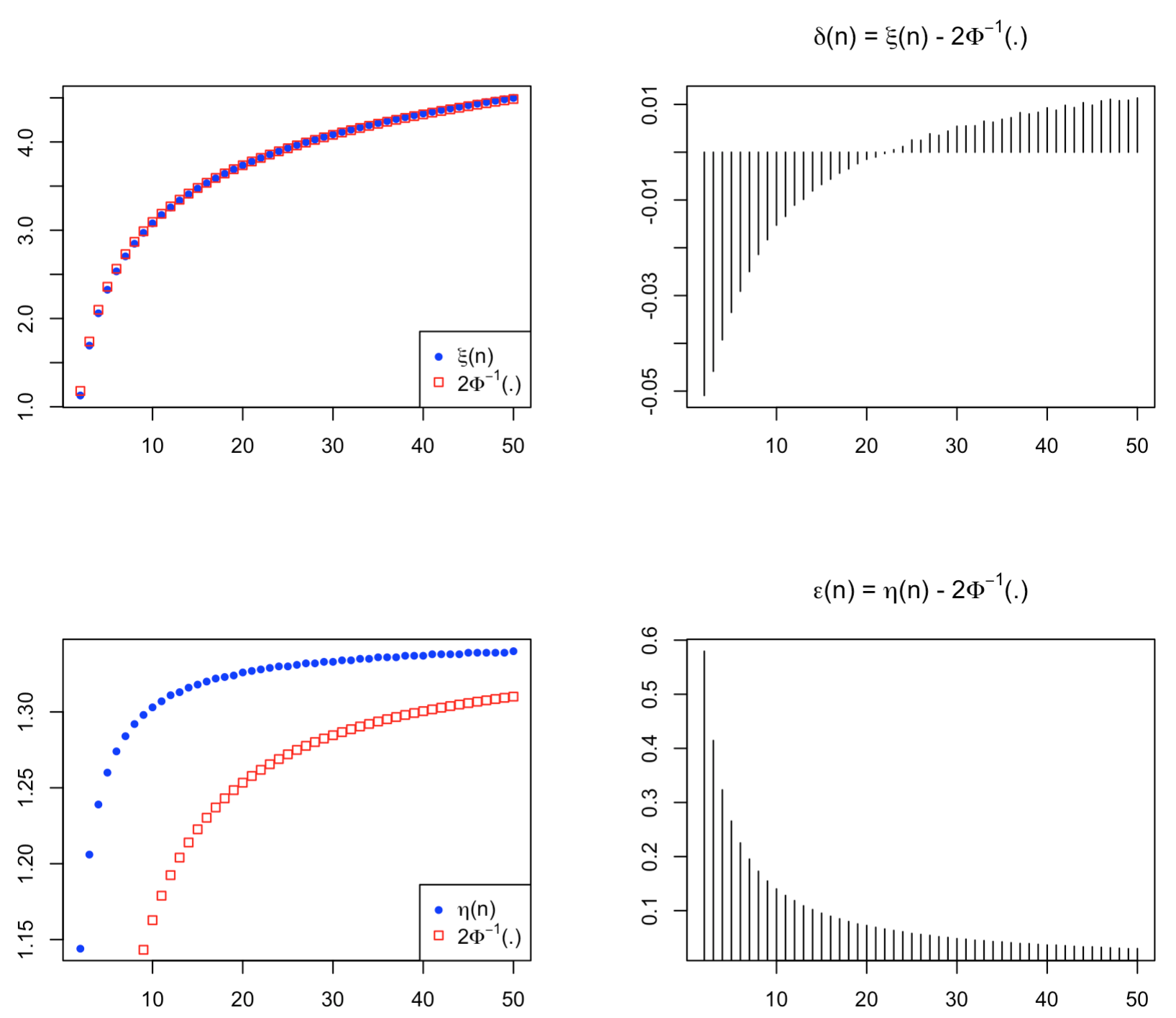
Figure 1: in the upper left panel, the blue bullets represent the $\xi(n)$ values as numerically computed in Table 1, while the red squares depict the function ${2\cdot\Phi^{-1}\left(\frac{n-0.375}{n+0.25}\right)}$. On the upper right panel, the residuals $\delta(n)$ are plotted. In the lower left panel, the blue bullets represent function $\eta(n)$ as listed in Table 2, while $2\cdot\Phi^{-1}\left(\frac{0.75n-0.125}{n+0.25}\right)$ are plotted with red squares. In the lower right panel, sticks describe residuals $\varepsilon(n)$.

In what follows, we assume that $n\geq 2$, being the case $n=1$ not practically relevant. All the following analyses are detailed in https://github.com/MassimoBorelli/sd. To start, one defines:

$$\delta(n):=\xi(n)-2\cdot\Phi^{-1}\left(\frac{n-0.375}{n+0.25}\right)$$

$$\varepsilon(n):=\eta(n)-2\cdot\Phi^{-1}\left(\frac{0.75n-0.125}{n+0.25}\right)$$

where $\xi(n)$ and $\eta(n)$ are the tabulated values in Tables 1 and 2 and $\Phi^{-1}$ is the upper z-th standard normal quantile function. A simple visual inspection to the above right sides plots shows that $\varepsilon(n)$ and $\delta(n)$ approximately differs by one order of magnitude. This is the reason why we start discussing $\varepsilon(n)$ within scenario $\mathbf{C}_{3}$.

2.1 Construction of epsilon(n)

Let us observe that $\varepsilon(n)>0,\forall n\in\mathbf{N}$; therefore it will be possible to consider logarithms. We claim that it is worth seeking two constants $a,b<0$ in order to set

$$\hat{\varepsilon}(n;a,b):=\exp\left(\frac{n}{a+b\cdot n}\right)>0$$

as a possible estimate of $\varepsilon(n)$. In fact, if the above statement hold, we would have that:

$$0>\frac{n}{a+b\cdot n}=\log\left(\hat{\varepsilon}(n)\right)$$

$$\frac{n}{\log\left(\hat{\varepsilon}(n)\right)}=a+b\cdot n<0$$

and therefore the change of variable $Y={n}/{\log\left(\hat{\varepsilon}(n)\right)}$ would yield to a linear relation:

$$Y=a+b\cdot n$$

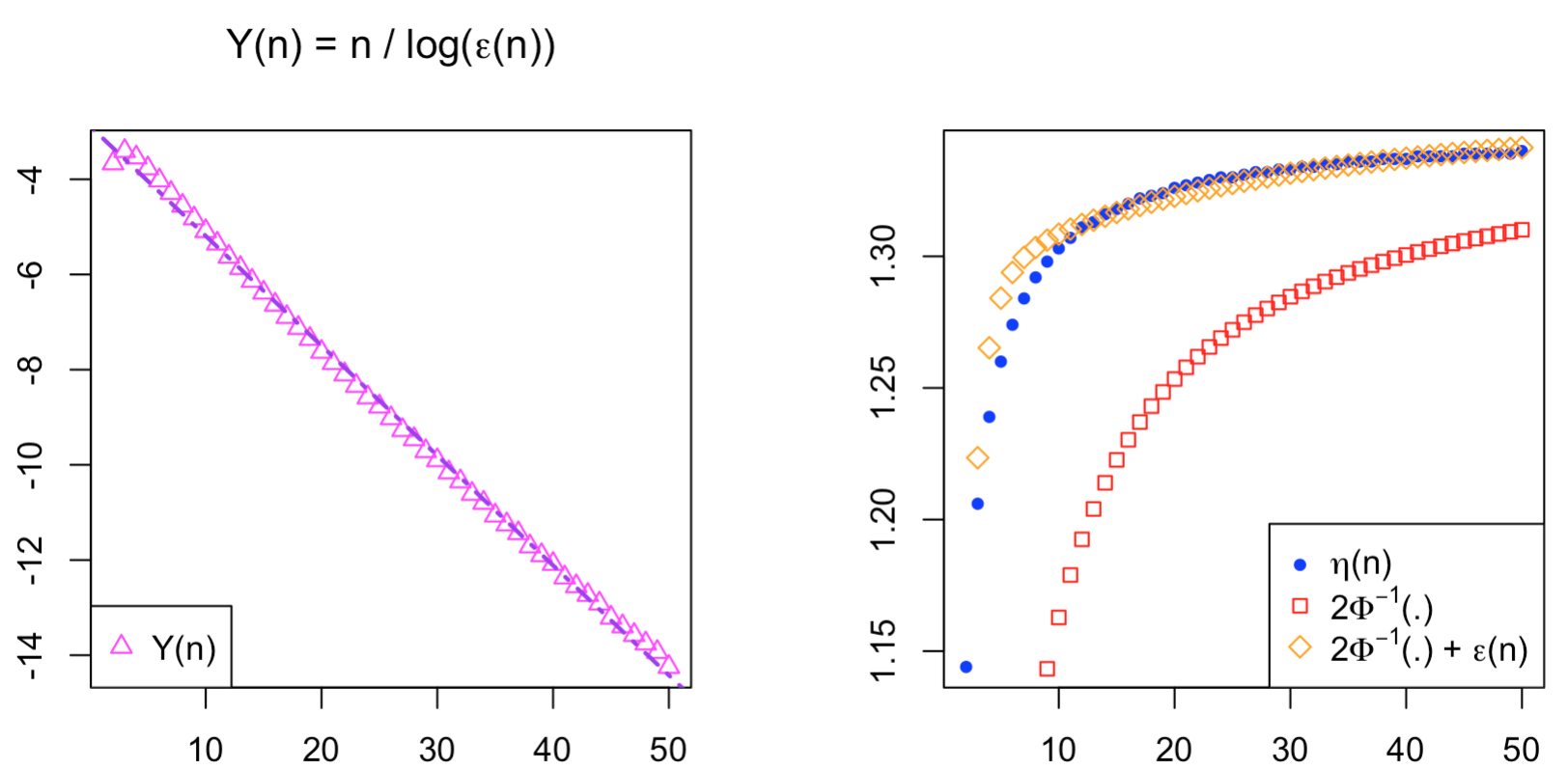
Figure 2: on the left, the linear behaviour of $Y(n)$ in magenta triangles; the dashed purple regression line is estimated. On the left, the blue bullets represent the $\xi(n)$ values, the red squares depict the function Wan et al., ${2\cdot\Phi^{-1}\left(\frac{0.75n-0.125}{n+0.25}\right)}$, while the orange diamonds plot our estimated proposal ${2\cdot\Phi^{-1}\left(\frac{0.75n-0.125}{n+0.25}\right)}+\exp\left(\frac{n}{-2.882-0.231\cdot n}\right)$.

As shown in Figure 2, if we plot $n/\log(\varepsilon(n))$ versus $n$, the pink triangles enhance the linear behaviour of $Y(n)$, justifying our initial claim: with a residual standard error of 0.141 and a determination coefficient $R^{2}=0.998$ the points appears to lie on the least mean squares $Y=-2.882-0.231\cdot n$ regression line. The summary below reported is an adaptation of the one provided by the lm function of R [R C14]:

	Estimate	Std. Error	t value	Pr($>$$|$t$|$)
$a$	-2.8822	0.0421	-68.48	$<$ 0.001
$b$	-0.2308	0.0014	-162.30	$<$ 0.001

Consequently, substituting $a$ and $b$ according to previous passages, we obtain a plausible estimate for $\varepsilon(n)$:

$$\hat{\varepsilon}(n):=\exp\left(\frac{n}{-2.882-0.231\cdot n}\right)$$ (5)

and therefore the $\eta(n)$ can be better approximated, according to the following relation:

$$\hat{\eta}(n)={2\cdot\Phi^{-1}\left(\frac{0.75n-0.125}{n+0.25}\right)+\exp\left(\frac{n}{-2.882-0.231\cdot n}\right)}$$

leading to the conclusive relation to estimate the standard deviation $\sigma$ within scenario $\mathbf{C}_{3}$:

$$\sigma\approx\frac{Q_{3}-Q_{1}}{2\cdot\Phi^{-1}\left(\frac{0.75n-0.125}{n+0.25}\right)+\exp\left(\frac{n}{-2.882-0.231\cdot n}\right)}$$ (6)

Observing that:

$$\lim_{n\to+\infty}\exp\left(\frac{n}{a+b\cdot n}\right)=\exp(1/b)$$

one concludes that $\hat{\varepsilon}(n)$ converges to $\exp(1/(-0.2307863...))=0.01312794...$ . Moreover, as one can verify that:

$$\sup_{2\leq n\leq 50}\left|\eta(n)-2\cdot\Phi^{-1}\left(\frac{0.75n-0.125}{n+0.25}\right)\right|\approx 0.580$$

$$\inf_{2\leq n\leq 50}\left|\eta(n)-2\cdot\Phi^{-1}\left(\frac{0.75n-0.125}{n+0.25}\right)\right|\approx 0.030$$

while:

$$\sup_{2\leq n\leq 50}\left|\eta(n)-\left[2\cdot\Phi^{-1}\left(\frac{0.75n-0.125}{n+0.25}\right)+\exp\left(\frac{n}{-2.882-0.231\cdot n}\right)\right]\right|\approx 0.030$$

$$\inf_{2\leq n\leq 50}\left|\eta(n)-\left[2\cdot\Phi^{-1}\left(\frac{0.75n-0.125}{n+0.25}\right)+\exp\left(\frac{n}{-2.882-0.231\cdot n}\right)\right]\right|<0.0002$$

our additive term (5) allows to gain at least one decimal figure in estimating $\eta(n)$ with respect to original equation (2).

The accuracy of $\hat{\eta}(n)$ can be easily improved. In fact, looking to the diagnostic plot of the linear model which led to relation 5, a non-negligible curvature in residuals clearly appears (see https://github.com/MassimoBorelli/sd for details), inducing not normality and heteroskedasticity. The situation can be amended, particularly if $3\leq n\leq 50$ with the second order relation:

$$\hat{\varepsilon}(n):=\exp\left(\frac{n}{-9.01647-0.23238\cdot(n-26)+0.00074\cdot(n-26)^{2}}\right)$$

which is characterized by a residual standard error of 0.035 on 45 degrees of freedom and a multiple R-squared equals to 0.9999, with nearly normal and homoskedastic residuals.

2.2 Construction of delta(n)

Let us start noting that the function $2\cdot\Phi^{-1}\left(\frac{n-0.375}{n+0.25}\right)$ proposed by Wan et al. [WWLT14] can be already considered a reliable approximation to $\xi(n)$, as

$$\sup_{2\leq n\leq 50}\left|\eta(n)-2\cdot\Phi^{-1}\left(\frac{n-0.375}{n+0.25}\right)\right|\approx 0.051$$

$$\inf_{2\leq n\leq 50}\left|\eta(n)-2\cdot\Phi^{-1}\left(\frac{n-0.375}{n+0.25}\right)\right|\approx 0.0003$$

Neverthelss, we investigated on the residuals $\delta(n)$ , $2\leq n\leq 50$ and their approximate derivative $\partial_{n}$, calculated by means of the central difference quotient (e.g. cfr. Stoer and Bulirsch [SB93], section 3.5 page 145)

$$\partial_{n}=\frac{\delta(n+1)-\delta(n-1)}{2}\;,\;3\leq n\leq 49$$

When plotting on the cartesian plane the sequence $\frac{1}{\partial_{n}}$ versus $n$, one can observe an approximate linear behaviour (apart from notable oscillations in the right graph tail). Therefore, we claim that setting:

$$Y=a+b\cdot\log(n)\equiv\log(A\cdot n^{b})$$

where $a=\log(A)$ one would have:

$$Y^{\prime}=\frac{d}{dn}Y=0+b\cdot\frac{1}{n}=\frac{b}{n}$$

that is:

$$n\propto\frac{b}{Y^{\prime}}$$

i.e. a linear behaviour of $b/Y^{\prime}$ versus $n$, as actually observed in Figure 3. Therefore, we set:

$$\hat{\delta}(n):=-0.0626+0.0197\cdot\log(n)$$ (7)

where $a$ and $b$ were again estimated by the lm function of R [R C14], with a residual standard error of 0.002 and a multiple $R^{2}=0.984$, according to the following summary:

	Estimate	Std. Error	t value	Pr($>$$|$t$|$)
$a$	-0.0626	0.0011	-54.66	$<$ 0.001
$b$	0.0197	0.0004	53.72	$<$ 0.001

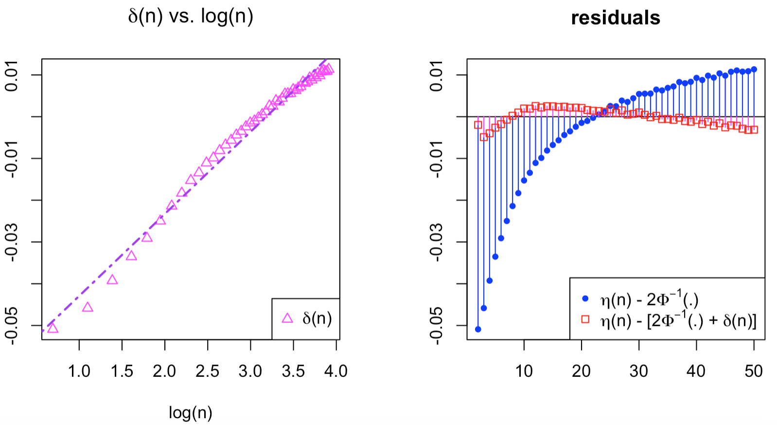
Figure 3: On the left, the the dashed purple regression line fitting the linear behaviour of $\hat{\delta}(n)$ versus $log(n)$ in magenta triangles. On the left, the blue sticks represent the measured $\delta(n)$ residuals, i.e. ${\eta(n)-2\cdot\Phi^{-1}\left(\frac{0.75n-0.125}{n+0.25}\right)}$; the red squares depict the residuals after correcting with $\hat{\delta}(n)$, i.e. $\eta(n)-\left({2\cdot\Phi^{-1}\left(\frac{0.75n-0.125}{n+0.25}\right)}+0.0197\cdot\log(n)-0.0626\right)$.

Consequently, with our proposed approximation (7) for $\delta(n)$, we conclude that in scenario $\mathbf{C_{1}}$ the function $\xi(n)$ can be approximated by:

$$\xi(n)\approx\hat{\xi}(n):=2\cdot\Phi^{-1}\left(\frac{n-0.375}{n+0.25}\right)+0.0197\log(n)-0.0626$$ (8)

yielding to the improved standard deviation estimating formula:

$$\sigma\approx\frac{b-a}{2\cdot\Phi^{-1}\left(\frac{n-0.375}{n+0.25}\right)+0.0197\log(n)-0.0626}$$ (9)

Lastly, we observe that also in this case one has approximately an improvement of one order of magnitude in decimal places:

$$\sup_{2\leq n\leq 50}\left|\xi(n)-\hat{\xi}(n)\right|\approx 0.005$$

$$\inf_{2\leq n\leq 50}\left|\xi(n)-\hat{\xi}(n)\right|<0.0002$$

3 Conclusions

In conclusion, in this short note we have verified that it is possible to estimate the standard deviation $\sigma$ when knowing the range $\left[a,b\right]$ and the sample size $n>1$ according to the following relation:

$$\sigma=\frac{b-a}{\xi(n)}$$ (10)

where:

$$\xi(n)\approx\left\{\begin{array}[]{ll}2\cdot\Phi^{-1}\left(\frac{n-0.375}{n+0.25}\right)+0.0197\log(n)-0.0626&\mbox{if $2\leq n\leq 50$}\\ 2\cdot\Phi^{-1}\left(\frac{n-0.375}{n+0.25}\right)&\mbox{if $n>50$}\end{array}\right.$$

while, if the quartiles $Q_{1}$ and $Q_{3}$ are known, together with the sample size $n>1$:

$$\sigma=\frac{Q_{3}-Q_{1}}{\eta(n)}$$ (11)

where:

$$\eta(n)\approx\left\{\begin{array}[]{ll}2\cdot\Phi^{-1}\left(\frac{0.75n-0.125}{n+0.25}\right)+\exp\left(\frac{n}{-2.882-0.231\cdot n}\right)&\mbox{if $2\leq n\leq 50$}\\ 2\cdot\Phi^{-1}\left(\frac{0.75n-0.125}{n+0.25}\right)&\mbox{if $n>50$}\end{array}\right.$$

Acknowledgments.

M.B. expresses his appreciation to professor Sergio L. Invernizzi of the Società dei Naturalisti e Matematici di Modena for his constructive suggestions, and lifelong teachings.

References

- [Bla15] Martin Bland. Estimating mean and standard deviation from the sample size, three quartiles, minimum, and maximum. International Journal of Statistics in Medical Research, 4(1):57, 2015.
- [Blo58] Gunnar Blom. Statistical estimates and transformed beta-variables. John Wiley & Sons, 1958.
- [CSWL17] Shein-Chung Chow, Jun Shao, Hansheng Wang, and Yuliya Lokhnygina. Sample size calculations in clinical research. CRC press, 2017.
- [HDH05] Stela Pudar Hozo, Benjamin Djulbegovic, and Iztok Hozo. Estimating the mean and variance from the median, range, and the size of a sample. BMC medical research methodology, 5(1):1–10, 2005.
- [R C14] R Core Team. R: A Language and Environment for Statistical Computing. R Foundation for Statistical Computing, Vienna, Austria, 2014.
- [SB93] Josef Stoer and Roland Bulirsch. Introduction to numerical analysis. Springer-Verlag, New York, 1993.
- [WWLT14] Xiang Wan, Wenqian Wang, Jiming Liu, and Tiejun Tong. Estimating the sample mean and standard deviation from the sample size, median, range and/or interquartile range. BMC medical research methodology, 14:1–13, 2014.