Abstract

Stochastic processes defined on integer valued state spaces are popular within the physical and biological sciences. These models are necessary for capturing the dynamics of small systems where the individual nature of the populations cannot be ignored and stochastic effects are important. The inference of the parameters of such models, from time series data, is difficult due to intractability of the likelihood; current methods, based on simulations of the underlying model, can be so computationally expensive as to be prohibitive. In this paper we construct a neural likelihood approximation for integer valued time series data using causal convolutions, which allows us to evaluate the likelihood of the whole time series in parallel. We demonstrate our method by performing inference on a number of ecological and epidemiological models, showing that we can accurately approximate the true posterior while achieving significant computational speed ups in situations where current methods struggle.

1 INTRODUCTION

Mechanistic models where the state consists of integer values are ubiquitous across all scientific domains, but particularly in the physical and biological sciences (van Kampen, 1992; Wilkinson, 2018). Integer valued states are important when the population being modelled is small and so the individual nature of the population cannot be ignored. Models of these types are used extensively for modelling in epidemiology (Allen, 2017), ecology (McKane and Newman, 2005), chemical reactions (Wilkinson, 2018), queuing networks (Breuer and Baum, 2005) and gene regulatory networks (Shea and Ackers, 1985), to name but a few examples. In working with mechanistic models, typically the main interest is in learning or inferring their parameters, rather than unobserved hidden states, as the parameters are directly related to the individual level mechanisms that drive the overall dynamics (Cranmer et al., 2020).

A combination of factors such as non-linear dynamics, partial observation and a complicated latent structure makes the inference of parameter posteriors a challenging problem. The likelihood is generally intractable and although methods that can sample from the exact posteriors exist—many based on simulation of the model itself—these can become computationally prohibitive in many situations (Doucet et al., 2015; Sherlock et al., 2015). Observations of a system with low noise are particularly challenging for simulation based methods, as the realisations that must be simulated are effectively rare events and hence generated with low probability (Del Moral et al., 2015; Drovandi and McCutchan, 2016; Black, 2019). Simulation based inference methods also scale poorly with ‘tall data’, which refers to large numbers of iid observations (Bardenet et al., 2017). In our context, such data arises from multiple short time series.

Our contribution—In this paper we construct a neural conditional density estimator (NCDE) for modelling the full likelihood of integer valued time series data. Specifically, we design an autoregressive model using a convolutional neural network (CNN) architecture with an explicit casual structure to model conditional likelihoods by a mixture of discretised logistic distributions. The likelihood approximation is trained using a modified sequential neural likelihood algorithm (Papamakarios et al., 2019) to jointly train the model and sample from an approximation of the posterior. This approach has three advantages over current methods:

• An autoregressive model allows us to approximate the likelihood of the entire time series, rather than fit to summary statistics calculated from the time series. Summary statistics are not suitable in many applications; for example, in outbreak data from small populations (Walker et al., 2017).

• Utilising causal convolutions means that evaluating the likelihood only requires a single neural network evaluation, rather than the sequential evaluation of a recurrent based architecture. This allows for fast training and MCMC sampling.

• Finally, our likelihood approximation is differentiable with respect to the parameters of the model, so a fast Hamiltonian Monte Carlo (HMC) kernel (Neal, 2011) can be used rather than a naïve random walk MCMC kernel.

We demonstrate our methods by performing inference on simulated data from two epidemic models, as well as a predator-prey model. The resulting posteriors are compared to those obtained using the exact sampling method particle marginal Metropolis Hastings (PMMH) (Andrieu et al., 2010). We are able to demonstrate accuracy in the posteriors generated from our method, suggesting that the autoregressive model is able to learn a good approximation of the true likelihood. Furthermore, our method is less computationally expensive to run in scenarios where PMMH struggles.

2 PROBLEM SETUP

Suppose we observe a time series of vectors of integers $\boldsymbol{y}_{1:n}$, assumed to come from a model parameterised by unknown parameters $\boldsymbol{\theta}$ that we wish to infer. In the typical Bayesian setting, we place a prior $p(\boldsymbol{\theta})$ on the model parameters and calculate or sample the posterior distribution $p(\boldsymbol{\theta}|\boldsymbol{y}_{1:n})\propto p(\boldsymbol{y}_{1:n}|\boldsymbol{\theta})p(\boldsymbol{\theta})$. The difficulty of doing this directly can be understood by considering how the observed data is generated from the model. The models we focus on evolve in continuous time, but if we assume that observations are made at discrete time intervals then the inference problem fits within the a state-space model (SSM) framework (Del Moral, 2004). SSMs are characterised by a latent state $\boldsymbol{x}_{i}$ and observations $\boldsymbol{y}_{i}$ corresponding to partial/noisy measurements of this state. The latent state has the law of a Markov process with transition kernel $p(\boldsymbol{x}_{i}|\boldsymbol{x}_{i-1},\boldsymbol{\theta})$, and the observations are conditionally independent of all previous states/observations given the current state (Del Moral, 2004). The joint likelihood for a SSM is given by

$$p(\boldsymbol{x}_{1:n},\boldsymbol{y}_{1:n}|\boldsymbol{\theta},\boldsymbol{x}_{0})=\prod_{i=1}^{n}p(\boldsymbol{y}_{i}|\boldsymbol{x}_{i})p(\boldsymbol{x}_{i}|\boldsymbol{x}_{i-1},\boldsymbol{\theta}).$$ (1)

For our setup the latent model is typically a continuous-time Markov chain (CTMC), also known as a Markov jump process, where the latent states are modelled by some subset of the positive integers (Ross, 2000; Wilkinson, 2018). Although in theory the transition kernel $p(\boldsymbol{x}_{i}|\boldsymbol{x}_{i-1},\boldsymbol{\theta})$ can be computed, in practice this is intractable for all but the simplest or smallest systems (Black et al., 2017; Sherlock, 2021). Hence the likelihood, obtained by marginalising $\boldsymbol{x}_{1:n}$ in Eq. (1), is intractable in general.

While the likelihood itself is intractable, simulation of CTMCs is trivial and accounts for their wide popularity (Gillespie, 1976). Many techniques which harness the ability to simulate from $p(\boldsymbol{y}_{1:n}|\boldsymbol{\theta})$ to perform (approximate) Bayesian inference exist, and such techniques fall under the umbrella of simulation based inference (SBI) (Cranmer et al., 2020). Our approach is to construct a NCDE that models the likelihood of the full discrete valued time series. This still relies on simulations of the model for training, but sidesteps the issues discussed in the introduction with rare events and tall data. Our likelihood approximator can also handle time series of random length, which may otherwise complicate methods based on summary statistics.

3 METHODS

In this section, we construct an autoregressive model to approximate $p(\boldsymbol{y}_{1:n}|\boldsymbol{\theta})$. The simplest version of the model works with univariate time series $y_{1:n}$, but we extend this to the multivariate case by using an additional masking procedure, which is described later. We also give an overview of sequential neural likelihood (SNL) (Papamakarios et al., 2019), discussing some adjustments to the algorithm to help increase consistency in the approximate posterior.

3.1 Autoregressive Model

Autoregressive models approximate the density of a time series $\boldsymbol{y}_{1:n}$ by modelling a sequence of conditionals, namely $p(\boldsymbol{y}_{i}|\boldsymbol{y}_{1:i-1})$ (Shumway and Stoffer, 2017), exploiting causality in the time series. The approximate density of $\boldsymbol{y}_{1:n}$ can be obtained by taking the product of the autoregressive model conditionals, in line with the factorisation

$$p(\boldsymbol{y}_{1:n})=p(\boldsymbol{y}_{1})\prod_{i=2}^{n}p(\boldsymbol{y}_{i}|\boldsymbol{y}_{1:i-1}).$$ (2)

For univariate time series, an autoregressive model can be constructed using a CNN which maps the input sequence $y_{1:n}$ to the sequence of conditionals in (2). A typical example is the model WaveNet (van den Oord et al., 2016), which uses a CNN constructed from dilated causal convolutions to ensure that the output sequence is compatible with (2). We take a similar approach, and construct an autoregressive model using (undilated) causal convolutions, which is advantageous when repeated likelihood evaluation is desired (such as within an MCMC scheme) as we can avoid sequential computations. If we use a kernel length of $k$ and $h$ hidden layers to construct the CNN, then its receptive field is $m=(k-1)(h+1)$, i.e. the $i^{\mathrm{th}}$ element in the output sequence is only dependent on $y_{i-m:i-1}$, making the CNN suitable for modelling conditionals of the form $p(y_{i}|y_{i-m:i-1})$. Dilating the convolutions lets $m$ grow exponentially with $h$ (van den Oord et al., 2016), however in the context of observations from a SSM, it is often the case that $p(y_{i}|y_{i-m:i-1})\approx p(y_{i}|y_{1:i-1})$ for moderately large $m$, provided that the observations are not dominated by noise. This can be justified with Lemma B.1 in the supplementary material. To aid with training of the model, we use residual connections in the hidden layers of the CNN, which are known to help stabilise training (He et al., 2016).

To model $p(y_{1:n}|\boldsymbol{\theta})$, we need the CNN to be dependent on $\boldsymbol{\theta}$. We approach this by using a shallow neural network to calculate a context vector $\mathbf{c}(\boldsymbol{\theta})$, and then add a linear transformation of $\mathbf{c}(\boldsymbol{\theta})$ to the output of each layer of the CNN (broadcasting across the time axis). Using $\mathbf{c}(\boldsymbol{\theta})$ instead of $\boldsymbol{\theta}$ can help the model learn to reparameterise the input parameters into a set of parameters that are identifiable and/or more directly influence the dynamics of the observations. Making every layer dependent on $\boldsymbol{\theta}$ allows for greater interaction between the model parameters and observations, and also admits conditionals where $\boldsymbol{\theta}$ has a varying influence across time. This is important for non-linear models where the model parameters can have an impact on the qualitative nature of the observation dynamics (Arnol’d and Gamkrelidze, 1994). Further details of the model architecture are given in Appendix A of the supplement.

To approximate the autoregressive model conditionals, we use a discretised mixture of logistic distributions (DMoL) with $c$ mixture components (Salimans et al., 2017). Denote the output of the CNN by $\boldsymbol{o}_{1:n}\in{}^{n\times 3c}$ and the autoregressive model conditionals by $q_{\psi}(y_{i}|y_{1:i-1},\boldsymbol{\theta})$, where $\psi$ are the neural network parameters. The shift, scale and mixture proportion parameters of $q_{\psi}(y_{i}|y_{1:i-1},\boldsymbol{\theta})$ are given by

$$\mu_{i,j} =y_{i-1}+o_{i,j},$$ (3a)

$$s_{i,j} =\mathrm{softplus}(o_{i,c+j})+\epsilon,$$ (3b)

$$(w_{i,1},\cdots,w_{i,c}) =\mathrm{softmax}\left((o_{i,2c+1},\cdots,o_{i,3c})\right),$$ (3c)

where $o_{i,j}$ is the $j^{\mathrm{th}}$ element of $\boldsymbol{o}_{i}$ and $\epsilon$ is a small constant for numerical stability which we take to be $10^{-6}$. When the conditionals have a restricted support, the logistic distribution can be truncated analytically, which increases computational efficiency. For some processes we alter the equations (3) to better reflect the particular structure of a model. For example, the epidemic models we use yield count data which is bounded above by the total population size $N$, hence we can scale $s_{i,j}$ by $(N-y_{i-1})/N$ to reflect the shrinking support of the conditionals over time.

Modelling the multivariate case, $p(\boldsymbol{y}_{i}|\boldsymbol{y}_{1:i-1},\boldsymbol{\theta})$, is more difficult as we must consider dependencies between the components of $\boldsymbol{y}_{i}$. We approach this problem by decomposing the conditional $p(\boldsymbol{y}_{i}|\boldsymbol{y}_{1:i-1},\boldsymbol{\theta})$ as

$$p(\boldsymbol{y}_{i}|\boldsymbol{y}_{1:i-1},\boldsymbol{\theta})=\prod_{j=1}^{d}p(y_{i,j}|y_{i,1:j-1},\boldsymbol{y}_{1:i-1},\boldsymbol{\theta}),$$ (4)

where $y_{i,j}$ is the $j^{\mathrm{th}}$ component of $\boldsymbol{y}_{i}$. Incorporating the autoregressive structure of (4) into the CNN entails masking the convolution kernels in every layer of the CNN. The masking procedure consists of zeroing out certain blocks of the weight matrices in the convolution kernels, and it is almost identical to the masking procedure used in the model MADE (Germain et al., 2015), but it is applied across time; details of the masking can be found in Appendix A. Note that it is also easy to extend the autoregressive model to handle mixed types of data. For example, if we want to incorporate categorical data, we can use (3) to calculate the conditionals for the integer data, and a softmax to calculate the conditionals for the categorical data. In particular, we use integer and binary data for experiments concerning outbreak data in Section 5, where the binary data $f_{i}$ is an indicator for a certain event taking place at time $i$.

3.2 Training

Denoting the likelihood under the autoregressive model by $q_{\psi}(\boldsymbol{y}_{1:n}|\boldsymbol{\theta})$, then we optimise the neural network parameters $\psi$ by minimising $\mathbb{E}_{\tilde{p}(\boldsymbol{\theta})}[D_{\mathrm{KL}}(p||q_{\psi})]$, where $p$ represents the true likelihood and $\tilde{p}(\boldsymbol{\theta})$ is some proposal distribution whose support contains the prior support. Equivalently, we minimise the negative log-likelihood

$$-\mathbb{E}_{\tilde{p}(\boldsymbol{\theta})p(\boldsymbol{y}_{1:n}|\boldsymbol{\theta})}\left[\log q_{\psi}(\boldsymbol{y}_{1:n}|\boldsymbol{\theta})\right].$$

This is a standard objective for learning conditional densities as it is minimised if and only if $q_{\psi}=p$ almost everywhere (Papamakarios et al., 2019). It follows that the objective is minimised if $q_{\psi}(\boldsymbol{y}_{i}|\boldsymbol{y}_{1:i-1},\boldsymbol{\theta})=p(\boldsymbol{y}_{i}|\boldsymbol{y}_{1:i-1},\boldsymbol{\theta})$, however we know that our autoregressive model is incapable of achieving this due to the finite receptive field. Instead, minimising this objective will cause the autoregressive model to target the finite memory approximation of the true conditionals $p(\boldsymbol{y}_{i}|\boldsymbol{y}_{i-m:i-1},\boldsymbol{\theta})$. This is formalised in Proposition B.2 in the supplement.

3.3 Sequential Neural Likelihood

Sequential neural likelihood (SNL) is a SBI algorithm which uses a NCDE as a surrogate for the true likelihood within a MCMC scheme (Papamakarios et al., 2019). The main issue that is addressed by SNL is how to choose the proposal distribution over parameters in the training dataset $\tilde{p}(\boldsymbol{\theta})$. Ideally, the proposal would be the posterior over the model parameters so that the surrogate likelihood is well trained in regions where the MCMC sampler is likely to explore, without wasting time learning the likelihood in other regions. Obviously the posterior is not available, so instead SNL iteratively refines $q_{\psi}$ by sampling additional training data over a series of rounds. The initial proposal is taken to be the prior, and subsequent proposals are taken to be an approximation of the posterior, which is sampled from using MCMC with the surrogate from the previous round as an approximation of the likelihood. We refer the reader to Papamakarios et al. (2019) for more details on SNL.

We use our autoregressive model $q_{\psi}(\boldsymbol{y}_{1:n}|\boldsymbol{\theta})$ within SNL to perform inference for the experiments described in Section 5. We make a modification to how we represent the SNL posterior, in that we run SNL over $r$ rounds, and keep a mixture of MCMC samples over the final $r^{\prime}<r$ rounds. We do this because sometimes the posterior statistics exhibit variability which does not settle down over the SNL rounds, so it can be hard to assess whether the final round is truly the most accurate. Instead we use an ensemble to average out errors present in any given round, which worked well in practice. Variability across the SNL rounds occurs mostly when the length of time series is random, presumably because the random lengths inflate variability in the training dataset.

4 RELATED WORK

Exact sampling methods

For observations from SMMs, there are MCMC algorithms that target the posterior directly. One such approach augments the parameter space with the latent variables, which are sampled jointly with the parameters (O’Neill and Roberts, 1999; Brooks et al., 2011). Another approach is to use pseudo marginal methods (Andrieu and Roberts, 2009), such as particle marginal Metropolis Hastings (PMMH) (Andrieu et al., 2010), which uses a particle filter to obtain an unbiased estimate of the likelihood (Del Moral, 2004). Data augmentation does not scale well, as the method requires sampling from a very high dimensional space, and correlations between the parameters and latent state slow down the mixing of the MCMC chain. PMMH is often more efficient than data augmentation, but its performance decreases significantly if the SSM has a high dimensional latent state, or when using large data sets, i.e. long time series or a large number of observations. (Bickel et al., 2008; Snyder, 2012; Chopin and Papaspiliopoulos, 2020). When observations are integer valued and assumed to have low noise, then PMMH can suffer even further since the particle filter must simulate realisations that are effectively rare events (Del Moral and Murray, 2015; Black, 2019).

Modelling the Likelihood of Time Series

Modelling the distribution of time series using autoregressive models is well studied, although much of the literature focuses on the context of probabilistic forecasting (Salinas et al., 2020; Chen et al., 2020; Rasul et al., 2021) or generative modelling (van den Oord et al., 2016; Vaswani et al., 2017). The methods in this paper are similar to those in WaveNet, which was designed as a generative model for audio (van den Oord et al., 2016). Chen et al. (2020) use causal convolutions for the purposes of time series forecasting, however they relax the autoregressive property to allow for more robust forecasts, but such a relaxation would not be appropriate for a surrogate likelihood. Rasul et al. (2021) model the likelihood of time series using a normalising flow (Kobyzev et al., 2021), based on a recurrent neural network architecture. Like our model, this has the ability to model conditionals with correlated features; unlike our model, this only works for continuous valued data and requires sequential evaluation.

Simulation Based Inference

In the original implementation of SNL, Papamakarios et al. (2019) use continuous valued summary statistics for experiments on discrete time series data. Such an approach may result in a loss of informative data, and furthermore it is not easy to construct such statistics for models where the discrete nature of the observations cannot be neglected. Greenberg et al. (2019) approach the problem of SBI by directly learning the posterior instead of the likelihood. Such an approach can be used flexibly with continuous or discrete time series data, however manipulations which are trivial for the likelihood (e.g. factoring over independent observations) must be reflected in the neural network architecture for the posterior density estimator. It follows that this method may be difficult to implement for some problems of interest, e.g. outbreak data from multiple households. Hermans et al. (2020) perform SBI by learning the ratio of the likelihood with a distribution independent of $\boldsymbol{\theta}$. This approach requires training a classifier to distinguish between $(\boldsymbol{y},\boldsymbol{\theta})\sim\tilde{p}(\boldsymbol{\theta})p(\boldsymbol{y}|\boldsymbol{\theta})$ and $(\boldsymbol{y},\boldsymbol{\theta})\sim\tilde{p}(\boldsymbol{\theta})\tilde{p}(\boldsymbol{y})$, where $\tilde{p}(\boldsymbol{\theta})$ is a proposal distribution and $\tilde{p}(\boldsymbol{y})$ is the $\boldsymbol{y}$ marginal of $\tilde{p}(\boldsymbol{\theta})p(\boldsymbol{y}|\boldsymbol{\theta})$. Since this approach models the likelihood up to a constant of proportionality, it is suitable for use within MCMC, and hence may also work for the problems of interest in this paper, provided that an appropriate classifier for a time series could be constructed.

5 EXPERIMENTS

We evaluate our methods on simulated data from three different models, comparing the results to the exact sampling method PMMH (Andrieu et al., 2010). The first two models we consider are epidemic models, namely the SIR and SEIAR model, the former being a simple but ubiquitous model in epidemiology (Allen, 2017), and the latter being a more complex model which admits symptomatic phases (Black, 2019). The third example is the predator-prey model described in McKane and Newman (2005).

We perform two sets of experiments using the SIR model; one set considers a single simulated outbreak in a population of size 50, and the other considers multiple independent observations from outbreaks within households (small closed populations). The experiments on the single outbreak serve as a proof of concept for our method, as PMMH can target the posterior for this data efficiently (Black, 2019). The experiments on household data allow us to assess the scalability of our method with an increasing number of independent time series, where PMMH does not scale well.

The SEIAR model experiments serve two purposes, one being to assess the accuracy of our method when trained on data from a more complex model whose likelihood includes complex relationships between the model parameters. The other purpose is to assess the scalability with the population size as done in Black (2019), as increasing population sizes generally causes the performance of PMMH to degrade due to combination of longer time series and larger state spaces. The predator-prey model experiments also serve two purposes, one being to assess our method on a model with multivariate observations, and the other being to assess the scalability with lowering observation errors, where PMMH generally performs poorly due to weight degeneracy (Del Moral and Murray, 2015).

We run SNL 10 times with a different random seed for every outbreak experiment, and 5 times for the predator prey model experiments. Each run of SNL uses 10 rounds with NUTS (Hoffman and Gelman, 2014) as the MCMC sampler, and using the final 5 rounds to represent the posterior. All models were constructed using JAX (Bradbury et al., 2018) and the MCMC was run using numpyro (Phan et al., 2019). We validate our method against PMMH: for all outbreak experiments we use the particle filter of Black (2019) as it is specifically designed for noise free outbreak data. For the predator-prey model, we use a bootstrap filter (Kitagawa, 1996).

To assess accuracy of our method, we compare the posterior means and standard deviations for each parameter obtained from PMMH and SNL. We compare the estimated posterior means relative to the prior standard deviation to account for variability induced by using wide priors. We also compare the ratio of the estimated standard deviations, shifted so that the metric is 0 when SNL is accurate:

$$\mathrm{M}=\frac{\mu_{\mathrm{SNL}}-\mu_{\mathrm{PMMH}}}{\sigma_{\mathrm{Prior}}},~{}\quad\mathrm{S}=\frac{\sigma_{\mathrm{SNL}}}{\sigma_{\mathrm{PMMH}}}-1.$$

All posterior pairs plots can be found in Appendix E for a qualitative comparison between the results. We assess the runtime performance of our method by calculating the effective sample size per second (ESS/s) averaged over the parameters, where we take the ESS for SNL to be an average of the ESS values obtained from the MCMC chains over the final 5 rounds. Detailed descriptions of the models and additional details for the experiments such as hyperparameters can be found in Appendix C.

5.1 SIR model

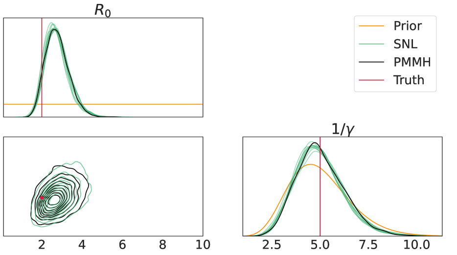
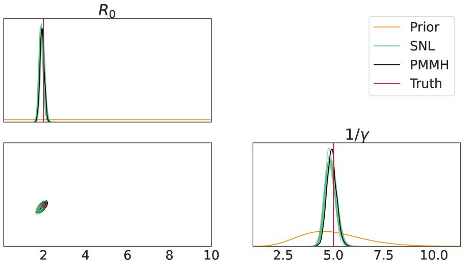
Figure 1: Posterior Pairs Plots for SIR Model Experiments. Left: single outbreak experiment from a population of $N=50$. Right: experiment using 500 households. For the univariate posteriors, we show all 10 runs of SNL, but only one of the runs for the bivariate posterior.

We first consider outbreak data from the SIR model (Allen, 2017). This model is a CTMC whose state at time $t$ counts the number of susceptible and infected individuals, $S_{t}$ and $I_{t}$ respectively. Equivalently, the state can be given in terms of two different counting processes: the total number of infections $Z_{1,t}=N-S_{t}$ and removals $Z_{2,t}=N-(S_{t}+I_{t})$, where $N$ is the population size. Our observed data is a time series of total case numbers $y_{1:n}$, where $y_{i}=Z_{1,i}$, equivalent to recording the number of new cases every day without error. Additionally, we assume that the outbreak has ended by day $n$ so the final size of the outbreak is equal to $y_{n}$. Since the outbreak never grows beyond $y_{n}$ cases, we can replace the full time series by $y_{1:\tau}$, where $\tau$ is random, and defined as the smallest $i$ with $y_{i}=y_{n}$. The task is to infer the two parameters of the model, $R_{0}>0$ and $1/\gamma>0$, using the data $y_{1:\tau}$. To model the randomness in $\tau$, we augment the autoregressive model with the binary sequence $f_{1:\tau}$, where $f_{i}=\delta_{i,\tau}$. The autoregressive model for this data is constructed by using $y_{1:\tau}$ as input to the CNN, and adding an additional output channel to the final layer of the CNN, which allows for calculation of $q_{\psi}(f_{i}|y_{1:i},f_{1:i-1},\boldsymbol{\theta})$. Using the multivariate formulation of the autoregressive model would be redundant, as by construction we always have $p(y_{i},f_{i}|y_{1:i-1},f_{1:i-1},\boldsymbol{\theta})=p(y_{i},f_{i}|y_{1:i-1},f_{i-1},\boldsymbol{\theta})$, and $f_{i-1}=0$ for any $i\leq\tau$; this fact and more details concerning the autoregressive model construction in these experiments are explained in Appendix C.2.

Single realisation

Our proof of concept example is a single observed outbreak in a population of size 50. The left of Figure 1 shows the posterior pairs plot of SNL compared to PMMH, which clearly shows that SNL provides an accurate approximation of the true posterior for this experiment; see Appendix D for a quantitative comparison. For this particular experiment, PMMH obtains an ESS/s of 69.38, which outperforms SNL with only 3.74. This is unsurprising, as we are not using a large amount of data and the particle filter we used was specifically designed to perform well for observations of this form.

Household data

Here, we mimic outbreak data collected from households (Walker et al., 2017), by generating $h$ observations with household sizes uniformly sampled between 2 and 7. We use values $h=100,~{}200$ and 500, assume that all households are independent, and that all outbreaks are governed by the same values of $R_{0}$ and $1/\gamma$, which have been chosen to be typical for this problem. The likelihood of an observation where $y_{\tau}=1$, or where the household size is 2, can be calculated analytically, so we incorporate these terms into inference manually. We therefore train the autoregresssive model to approximate $p(y_{1:\tau}|\boldsymbol{\theta},y_{\tau}>1)$ for population sizes of 3 through 7.

Table 1 shows the quantitative comparison between the two posteriors, indicating a negligible bias in the SNL means on average. The SNL variance appears to be slightly inflated on average, mainly for the $h=500$ experiments, though this is partly due to the PMMH variance shrinking with $h$, so the difference between the PMMH and SNL posteriors is still small, as indicated by the right of Figure 1. The ESS/s of SNL and PMMH are compared in the left panel of Figure 2, which clearly shows that SNL outperforms PMMH across each experiment, and that the drop off in SNL’s performance is less significant for increasing $h$. This is mainly because the autoregressive model can be evaluated efficiently on the observations in parallel.

Table 1: Comparison of SNL and PMMH posterior statistics for household data experiments. The values reported are the average over the 10 SNL runs and the maximum deviation from 0.

Param	$h$	M		S
		avg	max	avg	max
	100	-0.003	-0.02	0.01	-0.08
	200	-0.002	-0.02	0.02	0.13
$R_{0}$	500	-0.003	-0.02	0.04	0.11
	100	0.004	-0.10	0.02	0.10
	200	0.002	-0.05	0.06	0.15
$1/\gamma$	500	-0.03	-0.07	0.11	0.17

5.2 SEIAR model

Figure 2: Comparison of ESS/s for SNL and PMMH for all three models. The lines plotted for SNL are the averages over the runs, and the error bars correspond to the maximum and minimum. All plots are on a log-log scale. The horizontal axis of the left panel scales the observed dataset size, showing that our method has improved scaling compared to the gold standard PMMH. The horizontal axis of the middle panel scales the system size and similarly shows improved scaling. The horizontal axis of the right panel scales the observation accuracy, as discussed in Section 5.3. We observe the well-known phenomenon that PMMH runtime degrades with more accurate data, but SNL improves.

This more sophisticated outbreak model includes a latent exposure period, symptomatic phases and asymptomatic cases (Black, 2019). The state of the model can be given in terms of 5 counting processes $Z_{1,t},\,\ldots,\,Z_{5,t}$, which count the total number of exposures, pre-symptomatic cases, symptomatic cases, removals and asymptomatic cases respectively. In addition to $R_{0}$ and $1/\gamma$, the model has three extra parameters: $1/\sigma\geq 0$, $\kappa\in(0,1)$ and $q\in(0,1)$. The observations are of the same form as the SIR model observations, where the case numbers at day $i$ are given by $y_{i}=Z_{3,i}$, corresponding to counting the number of new symptomatic cases each day. With these observations, the likelihood has a complicated relationship between the parameters $R_{0}$ and $q$, which manifests as a banana shaped joint posterior. We assess our method on observations from populations of size $N=350,~{}500,~{}1000$ and 2000.

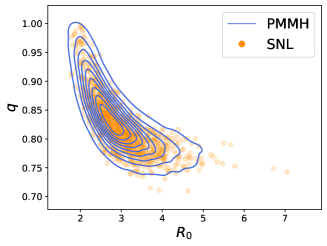
Figure 3: $(R_{0},q)$ joint posterior samples for SEIAR experiment with $N=500$.

Table 2 shows a comparison of the posterior statistics for the parameters $R_{0}$ and $\kappa$. The metrics for the other parameters are deferred to Appendix D. The bias in the mean value of $R_{0}$ is consistently small, but the standard deviations are slightly inflated, more so with larger population sizes. The $R_{0}$ posterior for these experiments is quite right skewed, and SNL produces posteriors which are slightly too heavy in the tail, which explains the inflated variance estimates. For $\kappa$, the posterior means do exhibit a noticeable bias, but the posterior standard deviations do not on average. The bias in $\kappa$ is lowest for the $N=500$ experiment, where the posterior has a mode near $\kappa=0$. The parameter $\kappa$ only has a weak relationship with the data, being the most informative near 0 or 1, hence the effect of $\kappa$ on the likelihood is presumably difficult to learn. This would explain the biases in the $\kappa$ posteriors, and would also explain why the $N=500$ experiment had the lowest bias on average. SNL manages to correctly reproduce the banana shaped posterior between $R_{0}$ and $q$, which can be seen for $N=500$ in Figure 3. In terms of runtime, the centre panel of Figure 2 shows that the performance of SNL drops off at a slower rate than PMMH with increasing $N$, and is noticeably faster for the $N=1000$ and 2000 experiments.

Table 2: Comparison of SNL and PMMH posterior statistics for $R_{0}$ and $\kappa$ in the SEIAR model.

Param	$N$	M		S
		avg	max	avg	max
	350	-0.003	-0.02	0.04	0.08
	500	0.005	0.09	-0.02	-0.09
	1000	0.05	0.08	0.13	0.20
$R_{0}$	2000	0.02	0.04	0.20	0.31
	350	0.20	0.32	0.01	0.04
	500	-0.08	-0.20	-0.06	-0.14
	1000	-0.16	-0.29	-0.0004	0.03
$\kappa$	2000	-0.25	-0.35	0.02	0.07

5.3 Predator-Prey model

Here, we consider data generated from the predator-prey model described in McKane and Newman (2005), which exhibits resonant oscillations in the predator and prey populations. The model is a CTMC with state $(P_{t},Q_{t})$ where $P_{t}$ and $Q_{t}$ are the numbers of predators and prey at time $t$ respectively. The model has 5 parameters, $b,d_{1},d_{2},p_{1},p_{2}>0$, which are the prey birth rate, predator death rate, prey death rate, and two predation rates respectively. The task is to infer these 5 parameters from predator and prey counts collected at discrete time steps, when any individual predator/prey has a probability $r$ (assumed to be fixed and known) of being counted. We use the values $0.5$, $0.7$ and $0.9$ for $r$, and all noisy observations are generated from a single underlying realisation, where we simulate the predator and prey populations over 200 time units, recording the population every 2 time units; see Appendix D for a plot of the data with $r=0.9$. We order the predators before the prey in the autoregressive model conditionals in Eq. (4).

Table 3 shows the comparison between the posterior statistics for the experiments with $r=0.9$, which suggests negligible differences between the posterior mean and standard deviations. It is also worth noting that SNL correctly reproduces a highly correlated posterior between $d_{1}$ and $p_{1}$. Furthermore, the $d_{2}$ posterior is almost indistinguishable from the prior, suggesting that the autoregressive model can learn to reparameterise $\boldsymbol{\theta}$ into a set of identifiable parameters and suppress dependence on unidentifiable parameters. The accuracy of SNL increases with increasing $r$ for this model (see Appendix D for the other metrics), which is unsurprising, as there is a higher ‘signal-to-noise ratio’ in the training data for larger $r$, which leads to training data which is more informative for $p(\boldsymbol{y}_{1:n}|\boldsymbol{\theta})$. This is in direct contrast to PMMH, where more noise makes the particle filter less prone to weight degeneracy. The right of Figure 2 shows that SNL is an order of magnitude more efficient than PMMH for these experiments, and the ESS/s does not drop off with increasing $r$.

Table 3: Comparison of SNL and PMMH posterior statistics in the predator prey model with $r=0.9$.

Param	M		S
	avg	max	avg	max
$b$	-0.03	-0.07	-0.04	0.11
$d_{1}$	0.01	0.03	-0.002	-0.05
$d_{2}$	-0.002	-0.12	0.01	0.10
$p_{1}$	0.01	0.02	-0.006	-0.05
$p_{2}$	-0.05	-0.10	-0.05	-0.08

6 DISCUSSION

In this paper we have constructed a surrogate likelihood model for integer valued time series data using an autoregressive model based on causal convolutions. We peform approximate inference using the surrogate with SNL, where the use of convolutions allows us to achieve efficient likelihood evaluation/differentiation within MCMC. We have demonstrated that our method produces good approximations of the parameter posterior, accurately reproducing many features of the posteriors obtained from exact sampling methods. Furthermore, we demonstrated significant reduction in computational expense in scenarios where exact sampling methods struggle; in particular with large numbers of observations, complex models, and low observation noise. Our method has negligible biases in the posterior means across experiments, with the exception of the parameter $\kappa$ in the SEIAR model. This parameter has a very weak relationship with the data except near $\kappa=0$ or 1, so it is unsurprising that it is difficult to learn. Our method always yielded posterior standard deviations which were either very close to that of PMMH, or slightly too large, suggesting that we generally avoid overconfident estimates, which can be a problem in simulation based inference (Hermans et al., 2022). Our method is also relatively robust to randomness within the algorithm, not showing any major differences over independent runs of SNL.

In practice, we found the choice of priors to be important. For example, in the predator prey model experiments, sometimes the MCMC chain would wander into a regions of very low prior density, resulting in a degenerate proposal. This was easily fixed by truncating the priors to only allow parameters in a physical range. Any surrogate likelihood based method could fall victim to such behaviour, however since we use comparatively high dimensional data in our method, it seems possible that it could be more susceptible to this behaviour. A potential drawback of our method on time series with a large number of features is that the autoregressive model requires an ordering in the features. Such an ordering may not be natural and therefore could require significant amounts of tuning. Furthermore, in general the number of hidden channels in the CNN grows linearly with the input dimension, so the computational complexity of evaluation generally grows quadratically with the input dimension.

This work assumes that conditioning a finite number of steps back in time is sufficient to model the conditionals. If longer range dependencies were important, then dilated causal convolutions (van den Oord et al., 2016) or self attention (Vaswani et al., 2017) could be employed to construct the autoregressive model. Self attention could also be beneficial for high dimensional time series, since it has linear complexity in the number of hidden features compared to the quadratic complexity of convolution layers. Another line of enquiry would be to develop better diagnostics to assess the results of SNL. The diagnostics used in Papamakarios et al. (2019) did not fit well with our integer valued data, nor did it fit well with the random length time series in the epidemic models. Studying how robust our method is to model misspecification would also be important future work, as any real data is unlikely to truly follow a specific model.

 

Supplementary Material

 

Appendix A FULL DETAILS OF AUTOREGRESSIVE MODEL

A.1 One dimensional inputs

A causal convolution layer $\ell:{}^{n\times d_{\mathrm{in}}}\to{}^{n\times d_{\mathrm{out}}}$ with convolution kernel $(W_{1},\cdots,W_{k})$ (where $W_{j}\in{}^{d_{\mathrm{out}}\times d_{\mathrm{in}}}$) and bias $\operatorname{\boldsymbol{b}}\in{}^{d_{\mathrm{out}}}$ is given by

$$\ell(\operatorname{\boldsymbol{z}}_{1:n})_{i}=\sum_{j=0}^{k-1}W_{k-j}\operatorname{\boldsymbol{z}}_{i-j}+\operatorname{\boldsymbol{b}},$$

where we define $\operatorname{\boldsymbol{z}}_{j}=0$ for $j<1$. To make the layer $\boldsymbol{\theta}$-dependent, we augment it with an additive transformation of $\boldsymbol{\theta}$. We first calculate a context vector from $\boldsymbol{\theta}$ using a shallow neural network (with activation $\sigma$)

$$\mathbf{c}(\boldsymbol{\theta})=W^{2}_{\mathbf{c}}\sigma(W^{1}_{\mathbf{c}}\boldsymbol{\theta}+\operatorname{\boldsymbol{b}}_{\mathbf{c}}).$$ (5)

We then use a linear transformation of $\mathbf{c}(\boldsymbol{\theta})$ to add $\boldsymbol{\theta}$ dependence to $\ell$:

$$\ell(\operatorname{\boldsymbol{z}}_{1:n},\mathbf{c}(\boldsymbol{\theta}))_{i}=W_{\boldsymbol{\theta}}\mathbf{c}(\boldsymbol{\theta})+\sum_{j=0}^{k-1}W_{k-j}\operatorname{\boldsymbol{z}}_{i-j}+\operatorname{\boldsymbol{b}}.$$ (6)

The size of the hidden layer and the output in (5) are both hyperparameters.

Using an activation function $\sigma:\real\to\real$, a residual block in the CNN is given by

$$\ell_{\mathrm{res}}(\operatorname{\boldsymbol{z}}_{1:n},\mathbf{c}(\boldsymbol{\theta}))_{i}=\operatorname{\boldsymbol{z}}_{i}+\ell^{(2)}\left(\sigma\left(\ell^{(1)}\left(\sigma(\operatorname{\boldsymbol{z}}_{1:n}\right),\mathbf{c}(\boldsymbol{\theta}))\right),\mathbf{c}(\boldsymbol{\theta})\right)_{i},$$ (7)

where $\ell^{(1)}$ and $\ell^{(2)}$ are of the form in (6), both having the same number of input/output channels for simplicity.

From (6), it can be seen that $\ell(\operatorname{\boldsymbol{z}}_{1:n},\mathbf{c}(\boldsymbol{\theta}))_{i}$ is dependent on $\operatorname{\boldsymbol{z}}_{i-(k-1):i}$. Defining $f(y_{1:n},\boldsymbol{\theta})$ as the composition of $h$ causal convolutions, it follows that $f(y_{1:n},\mathbf{c}(\boldsymbol{\theta}))_{i}$ is dependent on $y_{i-h(k-1):i}$. We remove dependence on $y_{i}$ by applying one further causal convolution $\ell_{\mathrm{f}}$, with the weight matrix $W_{k}$ masked out:

$$\ell_{\mathrm{f}}(\operatorname{\boldsymbol{z}}_{1:n},\mathbf{c}(\boldsymbol{\theta}))_{i}=W^{(\mathrm{f})}_{\boldsymbol{\theta}}\mathbf{c}(\boldsymbol{\theta})+\sum_{j=1}^{k-1}W^{(\mathrm{f})}_{k-j}\operatorname{\boldsymbol{z}}_{i-j}+\operatorname{\boldsymbol{b}}^{(\mathrm{f})},$$ (8)

noting that the summation begins at 1 instead of 0 as in (6). The notion of masking here is not so important, as we could equivalently use a shorter convolution kernel, but the notion becomes important when using multivariate time series. For conditionals with $c$ mixture components, the full CNN is a composition of a causal convolution layer which maps $y_{1:n}$ to a sequence with $d_{h}$ channels, $r$ residual blocks each with $d_{h}$ output channels, and finally a masked causal convolution as in (8) with $3c$ output channels. Overall, this CNN can condition as far back as $m=2(r+1)(k-1)$ steps in the input sequence. Evaluation of the CNN $\mathcal{N}_{\psi}(y_{1:n},\boldsymbol{\theta})$ and calculation of the logistic parameters from the output is given in Algorithm 1. Note that we assume that the initial observation $y_{0}$ is known, so that the shifts of $q_{\psi}(y_{1}|\boldsymbol{\theta},y_{0})$ can be calculated in the same form as the other shifts.

Algorithm 1 Evaluation of $\mathcal{N}_{\psi}(y_{1:n},\boldsymbol{\theta})$

Input: Time series with initial value $y_{0:n}$, first CNN layer $\ell$, $r$ residual blocks $\ell_{\mathrm{res}}^{(1)},\ldots,\ell_{\mathrm{res}}^{(r)}$, final masked CNN layer $\ell_{\mathrm{f}}$, neural network parameters $\psi$.

Output: Sequence of shift, scale and mixture proportions for a mixture of $c$ discretised logistic conditionals.

1:  Calculate context $\mathbf{c}\leftarrow W^{2}_{\mathbf{c}}\sigma(W^{1}_{\mathbf{c}}\boldsymbol{\theta}+\operatorname{\boldsymbol{b}}_{\mathbf{c}})$.

2:  Apply first layer $\operatorname{\boldsymbol{z}}_{1:n}\leftarrow\ell(y_{1:n},\mathbf{c})$.

3:  For $k=1,\ldots,r$ do

4:       Apply the $k^{\mathrm{th}}$ residual block $z_{1:n}\leftarrow\ell_{\mathrm{res}}^{(k)}(\operatorname{\boldsymbol{z}}_{1:n},\mathbf{c})$.

5:  Apply the final layer $\boldsymbol{o}_{1:n}\leftarrow\ell_{\mathrm{f}}(\operatorname{\boldsymbol{z}}_{1:n},\mathbf{c})$.

6:  Calculate the logistic parameters.

7:  For $i=2,\ldots,n$ do

8:       For $j=1,\ldots,c$ do

9:          Calculate the shifts $\mu_{i,j}\leftarrow\boldsymbol{o}_{i,j}+y_{i-1}$.

10:          Calculate the scales $s_{i,j}\leftarrow\mathrm{softplus}(\boldsymbol{o}_{i,j+c})+10^{-6}$.

11:          Calculate the mixture proportions $w_{i,j}\propto\exp(\boldsymbol{o}_{i,j+2c})$.

12:  Return $\boldsymbol{\mu}_{1:n}$, $\boldsymbol{s}_{1:n}$, $\boldsymbol{w}_{1:n}$.

A.2 Multidimensional inputs

Naively using a multidimensional time series $\boldsymbol{y}_{1:n}$ within Algorithm 1 would be sub-optimal, as we would end up ignoring correlations between the features in $\boldsymbol{y}_{i}$. Instead, we mask the convolution kernels in the causal convolution layers, so that we can calculate $q_{\psi}(y_{i,j}|y_{i,1},\ldots,y_{i,j-1},\boldsymbol{y}_{1:i-1},\boldsymbol{\theta})$ from the output of the CNN.

Assume $\boldsymbol{y}_{i}$ is $d$ dimensional, and for simplicity assume that the output of each residual block has $dp$ output channels, where $p$ is a positive integer. For $j=1,2$, define the following $d\times d$ block matrix

$$M_{j}=\begin{bmatrix}1_{p\times d_{j}}&0_{p\times d_{j}}&\cdots&0_{p\times d_{j}}\\ 1_{p\times d_{j}}&1_{p\times d_{j}}&\cdots&0_{p\times d_{j}}\\ \vdots&\ddots&&\vdots\\ 1_{p\times d_{j}}&1_{p\times d_{j}}&\cdots&1_{p\times d_{j}}\\ \end{bmatrix},$$

where $d_{1}=1$, $d_{2}=p$, i.e. $M_{j}$ is a block lower triangular matrix where all entries on and below the block diagonal are 1. The masked causal convolution appropriate for the hidden layers of the CNN is then defined by

$$\tilde{\ell}(\operatorname{\boldsymbol{z}}_{1:n},\boldsymbol{\theta})=W_{\boldsymbol{\theta}}\mathbf{c}(\boldsymbol{\theta})+(M_{j}\odot W_{k})\boldsymbol{y}_{k}+\sum_{l=1}^{k-1}W_{k-l}\operatorname{\boldsymbol{z}}_{i-l}+\operatorname{\boldsymbol{b}},,$$ (9)

where $j=1$ for the first layer, and $j=2$ for the causal convolutions within residual blocks. The mask ensures that the $d$ blocks of $p$ channels in the hidden layers of the CNN will each be dependent on a different sequence of features $y_{i,1},\ldots y_{i,j}$. If $\operatorname{\boldsymbol{z}}_{1:n}$ is the output of any hidden layer, then the elements $\operatorname{\boldsymbol{z}}_{i,1+(j-1)p},\ldots,\operatorname{\boldsymbol{z}}_{i,jp}$ are only dependent on $\boldsymbol{y}_{i}$ through the elements $y_{i,1},\ldots,y_{i,j}$. The CNN will output $3cd$ output channels, where each block of $d$ channels corresponds to $3c$ mixture of logistic parameters. To remove dependence of the $j^{\mathrm{th}}$ block of output channels on $y_{i,j}$, we apply a $d\times d$ block lower triangular mask matrix similar to $M_{j}$ to the final layer, but where the block diagonal set to zeros:

$$M=\begin{bmatrix}0_{3c\times p}&0_{3c\times p}&\cdots&0_{3c\times p}\\ 1_{3c\times p}&0_{3c\times p}&\cdots&0_{3c\times p}\\ \vdots&\ddots&&\vdots\\ 1_{3c\times p}&1_{3c\times p}&\cdots&0_{3c\times p}\\ \end{bmatrix}.$$ (10)

We recover the one-dimensional autoregressive model when $d=1$, as $M_{1}$ and $M_{2}$ are matrices of ones, and $M$ is a matrix of zeros. The same procedure holds for categorical components, though the block sizes in the mask (10) will need to be adjusted to reflect the correct number of parameters of the categorical distribution.

A.3 Discretised Logistic

The logistic distribution is a probability distribution supported on with probability density

$$p(x;\mu,s)=\frac{\exp\left(-\frac{x-\mu}{s}\right)}{s\left(1+\exp\left(-\frac{x-\mu}{s}\right)\right)^{2}},$$

where $\mu\in\real$ is a shift parameter and $s>0$ is a scale parameter. The logistic distribution enjoys the property that it has an analytic cumulative distribution function:

$$F(x;\mu,s)=\frac{1}{1+\exp\left(-\frac{x-\mu}{s}\right)}.$$

The significance of this is that is is possible to obtain an analytic expression for a discretised logistic distribution, i.e. if $X\sim\mathrm{Logistic}(\mu,s)$, then for $n\in\mathbb{Z}$

$$\Pr([X]=n)=F\left(n+\frac{1}{2};\mu,s\right)-F\left(n-\frac{1}{2};\mu,s\right),$$

where $[X]$ denotes rounding to the nearest integer.

A mixture of discretised logistics is used in Salimans et al. (2017), where an autoregressive model for image generation is described. In this work, we instead discretise $X\sim\mathrm{Logistic}(\mu,s)$ by calculating $\lfloor X\rfloor$, since all of our experiments required modelling distributions supported on the non-negative integers. For an integer $n\geq 0$ we therefore have

$$\Pr(\lfloor X\rfloor=n) =F\left(n+1;\mu,s\right)-F\left(n;\mu,s\right),$$ (11)

$$=\frac{\exp\left(-\frac{n-\mu}{s}\right)\left(1-\exp(-\frac{1}{s})\right)}{\left(1+\exp\left(-\frac{n+1-\mu}{s}\right)\right)\left(1+\exp\left(-\frac{n-\mu}{s}\right)\right)}.$$

It is also possible to analytically truncate the logistic distribution so that it is supported on $[a,b]$, simply by renormalising the probability density:

$$p(x;\mu,s,a,b) =\frac{p(x;\mu,s)}{F(b;\mu,s)-F(a;\mu,s)},$$ (12)

$$=\frac{\left(1+\exp\left(-\frac{b-\mu}{s}\right)\right)\left(1+\exp\left(-\frac{a-\mu}{s}\right)\right)}{\exp\left(-\frac{a-\mu}{s}\right)\left(1-\exp(-\frac{b-a}{s})\right)}p(x;\mu,s),$$

$$=C(a,b,\mu,s)p(x;\mu,s).$$

If $a,b\in\mathbb{Z}$ with $b>a$, then the logistic can be discretised and truncated by multiplying (11) by $C(a,b,\mu,s)$ from (12).

Appendix B ADDITIONAL TECHNICAL DETAILS

B.1 Finite Memory Approximation of Conditionals

In the main text we asserted that for a sufficiently large $m$, $p(\boldsymbol{y}_{i}|\boldsymbol{y}_{1:i-1})\approx p(\boldsymbol{y}_{i}|\boldsymbol{y}_{i-m:i-1})$ when $\boldsymbol{y}_{i}$ is defined by the observation process of a state space model. This can be justified with the following lemma:

Lemma B.1.

For $i>m+1$, define $\tilde{p}(\boldsymbol{x}_{i},\boldsymbol{x}_{i-m-1})=p(\boldsymbol{x}_{i},\boldsymbol{x}_{i-m-1}|\boldsymbol{y}_{i-m:i-1})$, $A(\boldsymbol{x})=\frac{p(\boldsymbol{y}_{i}|\boldsymbol{x})}{p(\boldsymbol{y}_{i}|\boldsymbol{y}_{i-m:i-1})}$
and $B(\boldsymbol{x})=\frac{p(\boldsymbol{y}_{1:i-m-1}|\boldsymbol{x}_{i-m-1})}{p(\boldsymbol{y}_{1:i-m-1}|\boldsymbol{y}_{i-m:i-1})}$. Then

$$\frac{p(\boldsymbol{y}_{i}|\boldsymbol{y}_{1:i-1})}{p(\boldsymbol{y}_{i}|\boldsymbol{y}_{i-m:i-1})}-1=\mathrm{Cov}_{\tilde{p}}(A(\boldsymbol{x}_{i}),B(\boldsymbol{x}_{i-m-1})).$$

Proof.

We begin by noting that

$$p(\boldsymbol{y}_{i}|\boldsymbol{y}_{1:i-1}) =\int p(\boldsymbol{y}_{i}|\boldsymbol{x}_{i})p(\boldsymbol{x}_{i}|\boldsymbol{y}_{1:i-1})d\boldsymbol{x}_{i},$$ (13)

which follows from the conditional independence property of SSMs. Expanding $p(\boldsymbol{x}_{i}|\boldsymbol{y}_{1:i-1})$ as to introduce the state $m+1$ steps in the past gives us

$$p(\boldsymbol{x}_{i}|\boldsymbol{y}_{1:i-1}) =\int p(\boldsymbol{x}_{i},\boldsymbol{x}_{i-m-1}|\boldsymbol{y}_{1:i-1})d\boldsymbol{x}_{i-m-1},$$

$$=\int p(\boldsymbol{x}_{i}|\boldsymbol{x}_{i-m-1},\boldsymbol{y}_{i-m:i-1})p(\boldsymbol{x}_{i-m-1}|\boldsymbol{y}_{1:i-1})d\boldsymbol{x}_{i-m-1},$$

$$=\int p(\boldsymbol{x}_{i}|\boldsymbol{x}_{i-m-1},\boldsymbol{y}_{i-m:i-1})\frac{p\left(\boldsymbol{x}_{i-m-1},\boldsymbol{y}_{1:i-m-1}|\boldsymbol{y}_{i-m:i-1}\right)}{p\left(\boldsymbol{y}_{1:i-m-1}|\boldsymbol{y}_{i-m:i-1}\right)}d\boldsymbol{x}_{i-m-1},$$

$$=\int p(\boldsymbol{x}_{i}|\boldsymbol{x}_{i-m-1},\boldsymbol{y}_{i-m:i-1})\frac{p\left(\boldsymbol{y}_{1:i-m-1}|\boldsymbol{x}_{i-m-1}\right)p\left(\boldsymbol{x}_{i-m-1}|\boldsymbol{y}_{i-m:i-1}\right)}{p\left(\boldsymbol{y}_{1:i-m-1}|\boldsymbol{y}_{i-m:i-1}\right)}d\boldsymbol{x}_{i-m-1},$$

$$=\int p(\boldsymbol{x}_{i},\boldsymbol{x}_{i-m-1}|\boldsymbol{y}_{i-m:i-1})\frac{p\left(\boldsymbol{y}_{1:i-m-1}|\boldsymbol{x}_{i-m-1}\right)}{p\left(\boldsymbol{y}_{1:i-m-1}|\boldsymbol{y}_{i-m:i-1}\right)}d\boldsymbol{x}_{i-m-1}.$$

Substituting the above into (13) we get

$$p(\boldsymbol{y}_{i}|\boldsymbol{y}_{1:i-1}) =~{} \mathbb{E}_{\boldsymbol{x}_{i},\boldsymbol{x}_{i-m-1}|\boldsymbol{y}_{i-m:i-1}}\left[p(\boldsymbol{y}_{i}|\boldsymbol{x}_{i})\frac{p(\boldsymbol{y}_{1:i-m-1}|\boldsymbol{x}_{i-m-1})}{p(\boldsymbol{y}_{1:i-m-1}|\boldsymbol{y}_{i-m:i-1})}\right],$$

$$=~{} \mathbb{E}_{\boldsymbol{x}_{i}|\boldsymbol{y}_{i-m:i-1}}\left[p(\boldsymbol{y}_{i}|\boldsymbol{x}_{i})\right]\mathbb{E}_{\boldsymbol{x}_{i-m-1}|\boldsymbol{y}_{i-m:i-1}}\left[\frac{p(\boldsymbol{y}_{1:i-m-1}|\boldsymbol{x}_{i-m-1})}{p(\boldsymbol{y}_{1:i-m-1}|\boldsymbol{y}_{i-m:i-1})}\right]$$

$$+\mathrm{Cov}_{\boldsymbol{x}_{i},\boldsymbol{x}_{i-m-1}|\boldsymbol{y}_{i-m:i-1}}\left(p(\boldsymbol{y}_{i}|\boldsymbol{x}_{i}),\frac{p(\boldsymbol{y}_{1:i-m-1}|\boldsymbol{x}_{i-m-1})}{p(\boldsymbol{y}_{1:i-m-1}|\boldsymbol{y}_{i-m:i-1})}\right),$$

$$=~{} p(\boldsymbol{y}_{i}|\boldsymbol{y}_{i-m:i-1})+\mathrm{Cov}_{\boldsymbol{x}_{i},\boldsymbol{x}_{i-m-1}|\boldsymbol{y}_{i-m:i-1}}\left(p(\boldsymbol{y}_{i}|\boldsymbol{x}_{i}),\frac{p(\boldsymbol{y}_{1:i-m-1}|\boldsymbol{x}_{i-m-1})}{p(\boldsymbol{y}_{1:i-m-1}|\boldsymbol{y}_{i-m:i-1})}\right).$$

Hence

$$\frac{p(\boldsymbol{y}_{i}|\boldsymbol{y}_{1:i-1})}{p(\boldsymbol{y}_{i}|\boldsymbol{y}_{i-m:i-1})}-1=\mathrm{Cov}_{\boldsymbol{x}_{i},\boldsymbol{x}_{i-m-1}|\boldsymbol{y}_{i-m:i-1}}\left(\frac{p(\boldsymbol{y}_{i}|\boldsymbol{x}_{i})}{p(\boldsymbol{y}_{i}|\boldsymbol{y}_{i-m:i-1})},\frac{p(\boldsymbol{y}_{1:i-m-1}|\boldsymbol{x}_{i-m-1})}{p(\boldsymbol{y}_{1:i-m-1}|\boldsymbol{y}_{i-m:i-1})}\right).$$

∎

Lemma B.1 shows that $p(\boldsymbol{y}_{i}|\boldsymbol{y}_{1:i-1})=p(\boldsymbol{y}_{i}|\boldsymbol{y}_{i-m:i-1})$ when $\boldsymbol{x}_{i}$ and $\boldsymbol{x}_{i-m-1}$ are uncorrelated given $\boldsymbol{y}_{i-m:i-1}$. Correlations of $\boldsymbol{x}_{i}$ and $\boldsymbol{x}_{i-m-1}$ should be small when the observations are sufficiently informative for the state, in the sense that $p(\boldsymbol{y}|\boldsymbol{x})\ll 1$ in a large region of latent space. This follows because

$$p(\boldsymbol{x}_{i-j}|\boldsymbol{y}_{i-m:i-j},\boldsymbol{x}_{i-m-1})\propto p(\boldsymbol{y}_{i-j}|\boldsymbol{x}_{i-j})p(\boldsymbol{x}_{i-j}|\boldsymbol{y}_{i-m:i-j-1},\boldsymbol{x}_{i-m-1}).$$

Hence by recursion, the effect of the observation process $p(\boldsymbol{y}|\boldsymbol{x})$ on $p(\boldsymbol{x}_{i}|\boldsymbol{y}_{i-m:i-1},\boldsymbol{x}_{i-m-1})$ roughly grows exponentially with $m$. It follows that the filtering posteriors $p(\boldsymbol{x}_{i-j}|\boldsymbol{y}_{i-m:i-j},\boldsymbol{x}_{i-m-1})$ will be negligible in most regions where $p(\boldsymbol{y}_{i-j}|\boldsymbol{x}_{i-j})$ is negligible, hence over time, the effect of $\boldsymbol{x}_{i-m-1}$ is overwhelmed by the sequence of observations, effectively removing its dependence in $p(\boldsymbol{x}_{i}|\boldsymbol{y}_{i-m:i-1},\boldsymbol{x}_{i-m-1})$.

B.2 Training the Conditionals

Proposition B.2.

Suppose $q_{\psi}(\boldsymbol{y}_{i}|\boldsymbol{y}_{1:i-1},\boldsymbol{\theta})=q_{\psi}(\boldsymbol{y}_{i}|\boldsymbol{y}_{i-m:i-1},\boldsymbol{\theta})$ and there exists a $\psi^{*}$ such that $q_{\psi^{*}}(\boldsymbol{y}_{i}|\boldsymbol{y}_{1:i-1},\boldsymbol{\theta})=p(\boldsymbol{y}_{i}|\boldsymbol{y}_{i-m:i-1},\boldsymbol{\theta})$. Then $D_{\mathrm{KL}}(p(\boldsymbol{y}_{1:n}|\boldsymbol{\theta})~{}||~{}q_{\psi}(\boldsymbol{y}_{1:n}|\boldsymbol{\theta}))$ is minimised when $\psi=\psi^{*}$.

Proof.

Let $q(\boldsymbol{y}_{1:n}|\boldsymbol{\theta})$ be a distribution of the form

$$q(\boldsymbol{y}_{1:n}|\boldsymbol{\theta})=q(\boldsymbol{y}_{1}|\boldsymbol{\theta})\prod_{i=2}^{n}q(\boldsymbol{y}_{i}|\boldsymbol{y}_{i-m:i-1},\boldsymbol{\theta}),$$

where we define $q(\boldsymbol{y}_{i}|\boldsymbol{y}_{i-m:i-1},\boldsymbol{\theta})\equiv q(\boldsymbol{y}_{i}|\boldsymbol{y}_{1:i-1},\boldsymbol{\theta})$ for $i\leq m$. The KL-divergence is given by

$$D_{\mathrm{KL}}(p(\boldsymbol{y}_{1:n}|\boldsymbol{\theta})||q(\boldsymbol{y}_{1:n}|\boldsymbol{\theta})) =\int\log\frac{p(\boldsymbol{y}_{1:n}|\boldsymbol{\theta})}{q(\boldsymbol{y}_{1:n}|\boldsymbol{\theta})}p(\boldsymbol{y}_{1:n}|\boldsymbol{\theta})d\boldsymbol{y}_{1:n},$$

$$=\int\left(\log\frac{p(\boldsymbol{y}_{1}|\boldsymbol{\theta})}{q(\boldsymbol{y}_{1}|\boldsymbol{\theta})}+\sum_{i=2}^{n}\log\frac{p(\boldsymbol{y}_{i}|\boldsymbol{y}_{1:i-1},\boldsymbol{\theta})}{q(\boldsymbol{y}_{i}|\boldsymbol{y}_{i-m:i-1},\boldsymbol{\theta})}\right)p(\boldsymbol{y}_{1:n}|\boldsymbol{\theta})d\boldsymbol{y}_{1:n},$$

$$=D_{\mathrm{KL}}(p(\boldsymbol{y}_{1}|\boldsymbol{\theta})||q(\boldsymbol{y}_{1}|\boldsymbol{\theta}))+\sum_{i=2}^{n}\int\log\frac{p(\boldsymbol{y}_{i}|\boldsymbol{y}_{1:i-1},\boldsymbol{\theta})}{q(\boldsymbol{y}_{i}|\boldsymbol{y}_{i-m:i-1},\boldsymbol{\theta})}p(\boldsymbol{y}_{1:i}|\boldsymbol{\theta})d\boldsymbol{y}_{1:i}.$$ (14)

Now, using the fact that

$$-\log x\geq 1-x\quad\text{with equality if and only if }x=1,$$

we have

$$\int\log\frac{p(\boldsymbol{y}_{i}|\boldsymbol{y}_{1:i-1},\boldsymbol{\theta})}{q(\boldsymbol{y}_{i}|\boldsymbol{y}_{i-m:i-1},\boldsymbol{\theta})}p(\boldsymbol{y}_{1:i}|\boldsymbol{\theta})d\boldsymbol{y}_{1:i} =\int\log\frac{p(\boldsymbol{y}_{i}|\boldsymbol{y}_{i-m:i-1},\boldsymbol{\theta})}{q(\boldsymbol{y}_{i}|\boldsymbol{y}_{i-m:i-1},\boldsymbol{\theta})}p(\boldsymbol{y}_{1:i}|\boldsymbol{\theta})d\boldsymbol{y}_{1:i}+\int\log\frac{p(\boldsymbol{y}_{i}|\boldsymbol{y}_{1:i-1},\boldsymbol{\theta})}{p(\boldsymbol{y}_{i}|\boldsymbol{y}_{i-m:i-1},\boldsymbol{\theta})}p(\boldsymbol{y}_{1:i}|\boldsymbol{\theta})d\boldsymbol{y}_{1:i},$$

$$=\int\log\frac{p(\boldsymbol{y}_{i}|\boldsymbol{y}_{i-m:i-1},\boldsymbol{\theta})}{q(\boldsymbol{y}_{i}|\boldsymbol{y}_{i-m:i-1},\boldsymbol{\theta})}p(\boldsymbol{y}_{1:i}|\boldsymbol{\theta})d\boldsymbol{y}_{1:i}+C_{i},$$

$$\geq C_{i}+\int\left(1-\frac{q(\boldsymbol{y}_{i}|\boldsymbol{y}_{i-m:i-1},\boldsymbol{\theta})}{p(\boldsymbol{y}_{i}|\boldsymbol{y}_{i-m:i-1},\boldsymbol{\theta})}\right)p(\boldsymbol{y}_{1:i}|\boldsymbol{\theta})d\boldsymbol{y}_{1:i},$$

$$=C_{i}+1-\int\frac{q(\boldsymbol{y}_{i}|\boldsymbol{y}_{i-m:i-1},\boldsymbol{\theta})}{p(\boldsymbol{y}_{i}|\boldsymbol{y}_{i-m:i-1},\boldsymbol{\theta})}p(\boldsymbol{y}_{i-m:i}|\boldsymbol{\theta})d\boldsymbol{y}_{i-m:i},$$

$$=C_{i}+1-\int q(\boldsymbol{y}_{i}|\boldsymbol{y}_{i-m:i-1},\boldsymbol{\theta})p(\boldsymbol{y}_{i-m:i-1}|\boldsymbol{\theta})d\boldsymbol{y}_{i-m:i},$$

$$=C_{i},$$

where equality holds if and only if $q(\boldsymbol{y}_{i}|\boldsymbol{y}_{i-m:i-1},\boldsymbol{\theta})=p(\boldsymbol{y}_{i}|\boldsymbol{y}_{i-m:i-1},\boldsymbol{\theta})$. Since this choice of conditionals minimises each term in the sum in (14), it follows that the KL-divergence is minimised for this choice of $q$, with value

$$D_{\mathrm{KL}}(p(\boldsymbol{y}_{1:n}|\boldsymbol{\theta})||q(\boldsymbol{y}_{1:n},\boldsymbol{\theta}))=\sum_{i=m+2}^{n}C_{i}.$$

∎

Appendix C ADDITIONAL EXPERIMENT DETAILS

C.1 Hyperparameters and Implementation Details

All experiments were performed using a single NVIDIA RTX 3060TI GPU, which provides a significant speed up over a CPU due to the use of convolutions. All instances of PMMH were written in the Julia programming language, and the particle filters were run on 16 threads to improve performance.

We used a kernel length of 5 for all experiments, and since all observations have relatively low to no noise, this was sufficient to ensure that $p(\boldsymbol{y}_{i}|\boldsymbol{y}_{i-m:i-1})\approx p(\boldsymbol{y}_{i}|\boldsymbol{y}_{1:i-1},\boldsymbol{\theta})$ for all experiments. We used 5 mixture components in all experiments. We found that more mixture components resulted in slower training without a significant increase in performance, and less would slightly worsen accuracy without much increase in speed. For the SIR/SEIAR model experiments, we used 64 hidden channels and 2/3 residual blocks. For the predator-prey model experiments, we used 100 hidden channels and 3 residual blocks. All of these hyperparameters were chosen initially to be relatively small, and were increased when necessary based on an pilot run of training, adding depth to the network over width since computational cost grows quadratically with width. We also used the same activation function for all experiments, namely the gaussian linear error unit (GeLU) (Hendrycks and Gimpel, 2016).

For all experiments, we used 90% of the data for training and the other 10% for validation. We used Adam with weight decay (Loshchilov and Hutter, 2017) as the optimiser, using a weight decay parameter of $10^{-5}$ and a learning rate of 0.0003. The only other form of regularisation which we used was early stopping, using a patience parameter of 30 for all experiments. For the SIR/SEIAR/predator-prey model experiments, we used a batch size of 1024/256/512 to calculate the stochastic gradients. We used a large batch size for the SIR model experiments, because in general each observation was quite short and therefore sparse of data. For the SEIAR model experiments, the autoregressive model was prone to getting stuck at a local minimum in the first round of training with too high a batch size, so presumably the stochasticity in the gradients helped to break through the local minimum.

For the SIR model experiment with a single observation and the SEIAR model experiments, we used a simulation budget of 60,000 samples, using 10,000 from the prior predictive in the first round, hence we drew 5,000 MCMC samples per round. For the household experiments, we used a simulation budget of 100,000 due to the shorter observations, hence we drew 9,000 MCMC samples per round. For the predator-prey model, we used a simulation budget of 25,000, using 10,000 from the prior predictive, hence we drew 1,500 MCMC samples per round. We dropped the simulation budget in the predator prey experiments, because the time series were much longer on average, and MCMC more expensive for this data. Additionally, we always drew an extra 200 samples at the beginning of MCMC, which were used in the warmup phase to tune the hyperparameters of NUTS, and then were subsequently discarded.

C.2 SIR Model

C.2.1 The Model

The SIR model is a CTMC which models an outbreak in a homogeneous population of fixed size $N$, classing each individual as either susceptible, infectious or removed (Allen, 2017). The model has state space

$$\left\{(S,I,R)\in\mathbb{Z}^{3}~{}|~{}S,I,R\geq 0,~{}S+I+R+N\right\},$$

and transition rates

$$(S,I,R) \to(S-1,I+1,R)\quad\text{at rate }\frac{\beta SI}{N-1},$$ (15)

$$(S,I,R) \to(S,I-1,R+1)\quad\text{at rate }\gamma I,$$ (16)

where $\beta>0$ is the transmissibility and $\gamma>0$ is the recovery rate. The SIR model can be recast in terms of two counting processes by using the transformations

$$Z_{1} =N-S,$$ (17)

$$Z_{2} =R,$$ (18)

where $Z_{1}$ and $Z_{2}$ count the number of times (15) and (16) occur respectively. The model parameters $(\beta,\gamma)$ can be reparameterised into more interpretable quantities $R_{0}=\beta/\gamma$ and $1/\gamma$, where the former is the average number of infections caused by a single infectious individual (when most of the population is susceptible), and the latter is the mean length of the infectious period (Allen, 2017).

C.2.2 Autoregressive Model Tweaks

We assume that there is one initial infection, and that we subsequently observe the number of new cases every day (without any noise), equivalent to observing $Z_{1}$ at a frequency of once per day. We also assume that the outbreak has reached completion, hence the final size of the outbreak $N_{F}$ can be measured. Using the data $(y_{1:n},n_{F})$, we can calculate the day at which the final size is reached:

$$\tau=\min\{i|y_{i}=n_{F}\}.$$

Clearly,

$$p\left(y_{1:n},N_{F}=n_{F}|\boldsymbol{\theta}\right)=p\left(y_{1:\tau},N_{F}=n_{F}|\boldsymbol{\theta}\right),$$

since case numbers can never grow beyond the final size. We can take this further and define indicator variables

$$f_{i}=\delta_{y_{i},n_{F}},$$

from which it is easy to see that

$$p(y_{1:\tau},N_{F}=n_{F}|\boldsymbol{\theta})=p(y_{1:\tau},f_{0:\tau}|\boldsymbol{\theta}),$$

where we need to include $f_{0}$ in case the outbreak never progresses from the initial infection. In the context of the autoregressive model, we decompose the conditionals $p(y_{i},f_{i}|y_{1:i},f_{1:i},\boldsymbol{\theta})$ as follows

$$p(y_{i},f_{i}|y_{1:i},f_{0:i},\boldsymbol{\theta}) =p(f_{i}|y_{1:i},f_{0:i-1},\boldsymbol{\theta})p(y_{i}|y_{1:i-1},f_{0:i-1},\boldsymbol{\theta}),$$

$$=p(f_{i}|y_{1:i},f_{i-1},\boldsymbol{\theta})p(y_{i}|y_{1:i-1},f_{i-1},\boldsymbol{\theta}),$$

since $f_{i-1}=0$ implies that $f_{k}=0$ for all $k<i-1$. Furthermore, since $f_{i}=1$ if and only if $i=\tau$, then it follows that $f_{i-1}=0$ for all $i\leq\tau$. It would therefore be redundant to make $q_{\psi}(y_{i},f_{i}|y_{1:i-1},f_{i-1},\boldsymbol{\theta})$ explicitly dependent on $f_{i-1}$, since $f_{i-1}=0$ always by construction. As a result, we only need to use $y_{1:\tau}$ as an input to the CNN. We do require a tweak to the output layer of the CNN, so that it outputs 16 parameters per conditional, 15 for the DMoL parameters, and one for $q_{\psi}(f_{i}|y_{1:i},f_{i-1},\boldsymbol{\theta})$. Since $f_{i}$ should be conditioned on $y_{i}$, we use a mask on the final causal convolution layer which has a similar structure to (10) in Appendix A. Explicitly, the mask matrix has 15 rows of zeros, followed by a single row of ones, ensuring that only the parameter corresponding to $q_{\psi}(f_{i}|y_{1:i},f_{i-1},\boldsymbol{\theta})$ is dependent on $y_{i}$, and the other 15 are not.

In practice, we do not need to include $f_{0}$ in our calculation with the autoregressive model, as $p(f_{0}|\boldsymbol{\theta})$ can be calculated analytically using the rates (15), (16) (Karlin and Taylor, 1975):

$$p(f_{0}|\boldsymbol{\theta})=\frac{f_{0}+(1-f_{0})R_{0}}{R_{0}+1}.$$ (19)

We therefore train the autoregressive model on samples conditioned on $N_{F}>1$, and define the surrogate likelihood to be

$$q_{\psi}(y_{1:n},n_{F}|\boldsymbol{\theta})\equiv p(f_{0}|\boldsymbol{\theta})q_{\psi}(y_{1:\tau},f_{1:\tau}|\boldsymbol{\theta},f_{0}=0).$$

This prevents us from wasting simulations on time series with 0 length, which are likely when $R_{0}$ is small. In principle, we could also calculate $p(N_{F}>t|\boldsymbol{\theta})$ for some threshold size $t$, and only train on simulations which cross this threshold, which would further reduce the number of short time series in the training data. This is possible largely due to the simplicity of the SIR model, and such a procedure generally becomes more difficult for CTMCs with a higher dimensional state space.

The final augmentation that we make to the autoregressive model concerns masking out certain terms of the form $\log q_{\psi}(f_{i}|y_{1:i},f_{i-1},\boldsymbol{\theta})$, which forces $q_{\psi}(f_{i}|y_{1:i},f_{i-1},\boldsymbol{\theta})=p(f_{i}|y_{1:i},f_{i-1},\boldsymbol{\theta})=1$. There are three scenarios where this is appropriate:

1. If $y_{i}=y_{i-1}$ and $f_{i}=0$, as we know that $N_{F}\neq y_{i-1}$, and the outbreak does not process over the interval $[i-1,i]$, so $f_{i}=0$ with probability 1.

2. If $y_{1}=1$, since we always have $N_{F}>1$ by construction.

3. If $y_{i}=N$, since this corresponds to the whole population becoming infected, therefore we have $N_{F}=N$ and $f_{i}=1$ with probability 1.

We calculate the context vector $\mathbf{c}((\beta,\gamma))$ using a shallow neural network with 64 hidden units and 12 output units, using a GeLU non-linearity. For the household experiments, we additionally concatenate a one-hot encoding of the household size to $(\beta,\gamma)$ before calculating $\mathbf{c}$, so that the autoregressive model can distinguish between household sizes. To obtain the logistic parameters from the output of the neural network $\boldsymbol{o}_{1:\tau}$, we calculate

$$\mu_{i,j} =o_{i,j}N+(1-o_{i,j})y_{i-1},$$

$$s_{i,j} =(N-y_{i-1})\mathrm{softplus}(o_{i,j+5})+\epsilon.$$

This encourages the shifts to lie in the support of the conditional $\{y_{i-1},\ldots,N\}$ (since $y_{i}$ is increasing), and allows the scales to be learnt in proportion to the width of the support of each conditional.

C.2.3 Training and Inference Details

For inference, we used a $\mathrm{Uniform}(0.1,10)$ prior on $R_{0}$ and a $\mathrm{Gamma}(10,2)$ prior on $1/\gamma$, where we truncate the prior of $1/\gamma$ so that it is supported on $[1,\infty)$. For the single observation experiment, we simulate the data using the Gillespie (1976) algorithm, running for a maximum length of 100 days, which ensures that approximately 99.9% of samples (estimated based on simulation) from the prior predictive reach their final size. We construct a binary mask for the simulations where $\tau<100$ so that values following $\tau$ do not contribute to the loss during training.

For the household experiments, we did not need to generate training data from households of size 2, as the likelihood of such observations can be calculated analytically. The case of $N_{F}=1$ is handled by (19), and if $N_{F}=2$ it can be shown that

$$p(y_{1:\tau},n_{F}=2|\boldsymbol{\theta},N_{F}>1)=e^{-\tau(\beta+\gamma)}\left(1-e^{-(\beta+\gamma)}\right).$$

The training data was generated from five realisations for a single value of $\boldsymbol{\theta}$, using a unique household size (between 3 and 7) for each of the realisations. We found that it was useful to increase the variance of the proposals generated from MCMC, as the proposals had small variance and sometimes this seemed to reinforce biases over the SNL rounds. We inflated the variance of the proposals by fitting a diagonal covariance Gaussian to the proposed samples (centred to have mean 0), and added noise from the Gaussian to the proposals, effectively doubling the variance of the proposals over the individual parameters.

For all experiments on the SIR model we, we used the particle filter given in Black (2019) within PMMH. For the single observation experiment, we used 20 particles, and the MCMC chain was run for 30,000 steps, which was sufficient for this experiment since the particle filter works particularly well on the SIR model. For the household experiments, we used 20, 40 and 60 particles for 100, 200 and 500 households respectively. We ran the MCMC chain for long enough as necessary to obtain an ESS of approximately 1000 or above for both parameters. Mixing of the MCMC chain slows down with increasing household numbers due to increasing variance in the log-likelihood estimate that must be offset by also increasing the number of particles. The covariance matrix for the Metropolis-Hastings proposal was tuned based on a pilot run for all experiments.

C.3 SEIAR Model

This model is another outbreak model, and is described in Black (2019). It is a CTMC with state space

$$\left\{(Z_{1},Z_{2},Z_{3},Z_{4},Z_{5})~{}|~{}Z_{1}\geq Z_{2}\geq Z_{3}\geq Z_{4}\geq 0,~{}Z_{1}\geq Z_{5}\geq 0,~{}Z_{1}+\cdots+Z_{5}=N\right\},$$

and transition rates

$$(Z_{1},Z_{2},Z_{3},Z_{4},Z_{5}) \to(Z_{1}+1,Z_{2},Z_{3},Z_{4},Z_{5})\quad\text{at rate }\frac{(N-Z_{1})(\beta_{p}(Z_{2}-Z_{3})+\beta_{s}(Z_{3}-Z_{4}))}{N},$$ (20)

$$(Z_{1},Z_{2},Z_{3},Z_{4},Z_{5}) \to(Z_{1},Z_{2}+1,Z_{3},Z_{4},Z_{5})\quad\text{at rate }q\sigma(Z_{1}-Z_{2}-Z_{5}),$$ (21)

$$(Z_{1},Z_{2},Z_{3},Z_{4},Z_{5}) \to(Z_{1},Z_{2},Z_{3}+1,Z_{4},Z_{5})\quad\text{at rate }\gamma(Z_{2}-Z_{3}),$$ (22)

$$(Z_{1},Z_{2},Z_{3},Z_{4},Z_{5}) \to(Z_{1},Z_{2},Z_{3},Z_{4}+1,Z_{5})\quad\text{at rate }\gamma(Z_{3}-Z_{4}),$$ (23)

$$(Z_{1},Z_{2},Z_{3},Z_{4},Z_{5}) \to(Z_{1},Z_{2},Z_{3},Z_{4},Z_{5}+1)\quad\text{at rate }(1-q)\sigma(Z_{1}-Z_{2}-Z_{5}).$$ (24)

The event (20) represents a new exposure, (21) represents an exposure becoming infectious (but pre-symptomatic), (22) represents a pre-symptomtic individual becoming symptomatic, (23) represents a recovery, and (24) represents an exposure who becomes asymptomatic (and not infectious). The parameters of the model are the transmissibilities attributed to the pre-symptomatic and symptomatic population $\beta_{p},\beta_{s}>0$, the rate of leaving the exposed class $\sigma>0$, the rate of leaving the (pre)symptomatic infection class $\gamma>0$, and the probability of becoming infectious $q\in(0,1)$. We follow Black (2019) and reparameterise the model in terms of the parameters $R_{0}=(\beta_{p}+\beta_{s})/q\gamma$, $1/\sigma$, $1/\gamma$, $\kappa=\beta_{p}/(\beta_{p}+\beta_{s})$ and $q$. We use the same parameters to generate the observations and priors that were used in Black (2019): $R_{0}=2.2$, $1/\gamma=1$, $1/\sigma=1$, $\kappa=0.7$ and $q=0.9$, and priors

$$R_{0} \sim\mathrm{Uniform}(0.1,8),$$

$$\frac{1}{\sigma} \sim\mathrm{Gamma}(10,10),$$

$$\frac{1}{\gamma} \sim\mathrm{Gamma}(10,10),$$

$$\kappa \sim\mathrm{Uniform}(0,1),$$

$$q \sim\mathrm{Uniform}(0.5,1),$$

truncating the priors for $1/\sigma$ and $1/\gamma$ to have support $[0.1,\infty)$ and $[0.5,\infty)$ respectively.

The observations are given by the values of $Z_{3}$ at discrete time steps, corresponding to the number of new symptomatic individuals per day, as well as the final size $N_{F}$. We handle the final size data in the same way as discussed for the SIR model, but we include $f_{0}$ for this model, as $p(N_{F}=1|\boldsymbol{\theta})$ is more difficult to calculate due to the asymptomatic individuals. The initial state is taken to be $(Z_{1},Z_{2},Z_{3},Z_{4},Z_{5})=(1,1,0,0,0)$, which we simulate forward using the Gillespie algorithm until $Z_{3}=1$, after which we begin recording the values of $y_{i}$ at integer time steps. For population sizes of 350, 500, 1000 and 2000, we generate time series of maximum length 70, 80, 100 and 110 respectively. This ensured that at least 99% of samples from the prior predictive reached their final size (estimated by simulation). The autoregressive model follows the exact same construction as given for the SIR model experiments, except that we rescale the time series by the population size before inputting to the CNN. We also divide $y_{1:\tau}$ by $N$ before inputting to the CNN, which helps to stabilise training.

For PMMH, we used the particle filter given in Black (2019), using 70, 80, 100 and 120 particles for population sizes of 350, 500, 1000 and 2000 respectively. The MCMC chain was run until all parameters had an ESS of approximately 1000 or above, and the proposal covariance matrix was estimated based on a pilot run.

C.4 Predator-Prey Model

The predator-prey model that we use is described in McKane and Newman (2005). For large populations in predator-prey models, it is often sufficient to consider a deterministic approximation via an ODE. For this model, the corresponding ODE has a stable fixed point, which makes it incapable of exhibiting the cyclic behaviour seen in e.g. the Lotka-Volterra model (Wilkinson, 2018). In the stochastic model however, there is a resonance effect which causes oscillatory behaviour. Unlike predator-prey models with limit cycle behaviour, in this model the dominant frequencies in the oscillations have a random contribution to the trajectory, which causes greater variability among the realisations for a fixed set of parameters.

The model is a CTMC which represents the population dynamics of a predator population of size $P$ and a prey population of size $Q$. The state space given by

$$\left\{(P,Q)\in\mathbb{Z}^{2}~{}|~{}0\leq P,Q\leq K,~{}P+Q\leq K\right\},$$

where $K\geq 0$ is a carrying capacity parameter. The transition rates are given by

$$(P,Q) \to(P-1,Q)\quad\text{at rate }d_{1}P,$$ (25)

$$(P,Q) \to(P,Q+1)\quad\text{at rate }2b\frac{Q}{K}(K-P-Q),$$ (26)

$$(P,Q) \to(P,Q-1)\quad\text{at rate }2p_{2}\frac{PQ}{K}+d_{2}Q,$$ (27)

$$(P,Q) \to(P+1,Q-1)\quad\text{at rate }2p_{1}\frac{PQ}{K},$$ (28)

where $b,d_{1},d_{2},p_{1},p_{2}>0$ are the parameters of the model. To simulate the data, we use parameters $b=0.26$, $d_{1}=0.1$, $d_{2}=0.01$, $p_{1}=0.13$, $p_{2}=0.05$. We use informative priors on $b$, $d_{1}$ and $d_{2}$, assuming that reasonable estimates can be obtained based on observing the two individual species. In particular we use

$$\log b \sim N(\log 0.25,0.25),$$

$$\log d_{1} \sim N(\log 0.1,0.5),$$

$$\log d_{2} \sim N(\log 0.01,0.5),$$

truncating each prior to have support $(-\infty,0]$. For the two predation parameters, we use priors

$$p_{1} \sim\mathrm{Exponential}(0.1),$$

$$p_{2} \sim\mathrm{Exponential}(0.05),$$

where we truncate the prior of $p_{1}$ so that it is supported on $[0.01,\infty)$. To simulate the realisation for the observations, we use a carrying capacity of $K=800$ and initial condition $(250,250)$. We then run the Gillespie algorithm over 200 time steps, taking $\boldsymbol{y}^{\prime}_{i}=(P_{2i},Q_{2i})$, and apply observation error to generate the observations, namely

$$y_{i,1} \sim\mathrm{Binomial}(y^{\prime}_{i,1},r),$$

$$y_{i,2} \sim\mathrm{Binomial}(y^{\prime}_{i,2},r),$$

for $r=0.5,~{}0.7,~{}0.9$.

To generate the training data, we firstly infer the initial condition from the noisy initial observation $\boldsymbol{y}_{0}$. In particular, we assume $p(P_{0})\propto 1$ and $p(Q_{0})\propto 1$, from which it is easy to derive the posterior $p((P_{0},Q_{0})|\boldsymbol{y}_{0})$:

$$\left(P_{0}-y_{0,1}\right)|\boldsymbol{y}_{0} \sim\mathrm{NegativeBinomial}(y_{0,1}+1,r),$$

$$\left(Q_{0}-y_{0,2}\right)|\boldsymbol{y}_{0} \sim\mathrm{NegativeBinomial}(y_{0,2}+1,r).$$

We then generate the training data in the same way we produced the observations. No tweaks are made to the autoregressive model, though we do divide $\boldsymbol{y}_{1:100}$ by 60 before inputting to the CNN, and multiply the shifts (before adding $\boldsymbol{y}_{i-1}$) and scales by 60. We do this because the standard deviation across the time axis for samples from the prior predictive was estimated to be approximately 60. We also tried rescaling the input/output by larger values, but this generally resulted in less stable training and slower MCMC iterations. We do not centre the inputs, because if $y_{i,j}=0$ for multiple time steps in a row, then this implies that an extinction has likely occurred, hence zeroing the weights associated with $y_{i,j}$ in the first layer should correspond to the model learning the dynamics of the individual species. If we centred the data, then extinctions would not correspond to zeroing the weights. We also attempted to order the prey before the predators in the autoregressive model, but found that there was not a large difference between the two orderings.

For PMMH, we used a bootstrap particle filter (Kitagawa, 1996), using 100, 200 and 250 particles for $r=0.5,~{}0.7$ and 0.9 respectively. We used 180,000 MCMC iterations for each experiment, which produced an ESS of greater than 500 for all parameters. Generating a large ESS for this data is difficult due to the extremely high posterior correlation between $d_{1}$ and $p_{1}$, and the computational time per MCMC iteration is quite high for these experiments. We estimated the covariance matrix for the MCMC kernel from a prior SNL run, and tuned further based on a pilot run. Without the SNL run to inform the initial covariance matrix, tuning the MCMC proposal would likely take huge amounts of computational time, since a proposal with diagonal covariance would mix extremely slowly with the highly correlated parameters in the posterior.

Appendix D ADDITIONAL RESULTS

D.1 Posterior Metrics

Table 4: Comparison of SNL and PMMH posterior statistics for the SIR model.

Param	M		S
	avg	max	avg	max
$R_{0}$	0.00007	-0.0034	0.036	0.068
$1/\gamma$	-0.029	-0.087	0.019	0.073

Table 5: Comparison of SNL and PMMH posterior statistics for $1/\sigma$, $1/\gamma$ and $q$ in the SEIAR model.

Param	$N$	M		S
		avg	max	avg	max
	350	0.04	0.10	0.03	0.07
	500	0.01	0.08	-0.01	-0.05
	1000	0.02	0.08	0.02	0.05
$1/\sigma$	2000	-0.007	-0.05	0.04	0.07
	350	0.07	0.20	0.03	0.06
	500	0.08	0.30	0.03	0.08
	1000	0.05	0.17	0.03	0.06
$1/\gamma$	2000	0.04	0.10	0.03	0.10
	350	-0.03	-0.06	0.02	0.06
	500	-0.05	-0.12	-0.02	-0.12
	1000	-0.07	-0.12	-0.02	-0.06
$q$	2000	-0.02	-0.07	0.06	0.08

Table 6: Comparison of SNL and PMMH posterior statistics predator prey model experiments.

Param	$r$	M		S
		avg	max	avg	max
	0.5	-0.09	-0.22	-0.02	-0.10
$b$	0.7	-0.05	-0.11	-0.009	-0.06
	0.5	-0.08	-0.18	-0.01	-0.08
$d_{1}$	0.7	-0.003	-0.02	0.03	0.08
	0.5	-0.00001	-0.14	-0.08	-0.16
$d_{2}$	0.7	0.04	0.12	0.05	0.17
	0.5	-0.06	-0.13	-0.01	-0.09
$p_{1}$	0.7	-0.0003	-0.01	0.03	0.08
	0.5	0.02	0.13	0.02	0.07
$p_{2}$	0.7	-0.06	-0.08	-0.11	-0.17

D.2 Runtimes

Table 7: ESS/s values from PMMH versus SNL for household data experiments. Recall that we report the ESS/s value for SNL by averaging the ESS over the final 5 rounds.

$h$	PMMH ESS/s	SNL ESS/s
		avg	min	max
100	2.33	3.67	3.37	4.00
200	0.70	3.28	3.03	3.44
500	0.25	2.38	2.25	2.57

Table 8: ESS/s values from PMMH versus SNL for SEIAR experiments. Recall that we report the ESS/s value for SNL by averaging the ESS over the final 5 rounds.

$N$	PMMH ESS/s	SNL ESS/s
		avg	min	max
350	1.94	2.55	2.24	2.96
500	1.65	1.78	1.60	1.90
1000	0.50	1.50	1.29	1.62
2000	0.20	1.23	1.08	1.39

Table 9: ESS/s values from PMMH versus SNL for predator-prey experiments. Recall that we report the ESS/s value for SNL by averaging the ESS over the final 5 rounds.

$r$	PMMH ESS/s	SNL ESS/s
		avg	min	max
0.5	0.034	0.33	0.29	0.37
0.7	0.027	0.51	0.48	0.56
0.9	0.015	0.45	0.34	0.50

Appendix E ADDITIONAL PLOTS

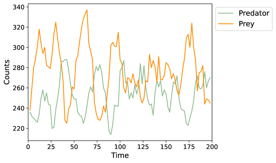
Figure 4: Predator and prey counts for $r=0.9$. Both populations oscillate around an equilibrium in a somewhat irregular fashion.

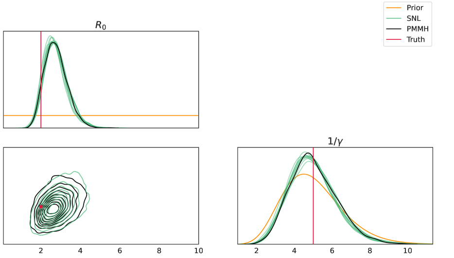
Figure 5: Posterior pairs plot for single observation from SIR model experiment.

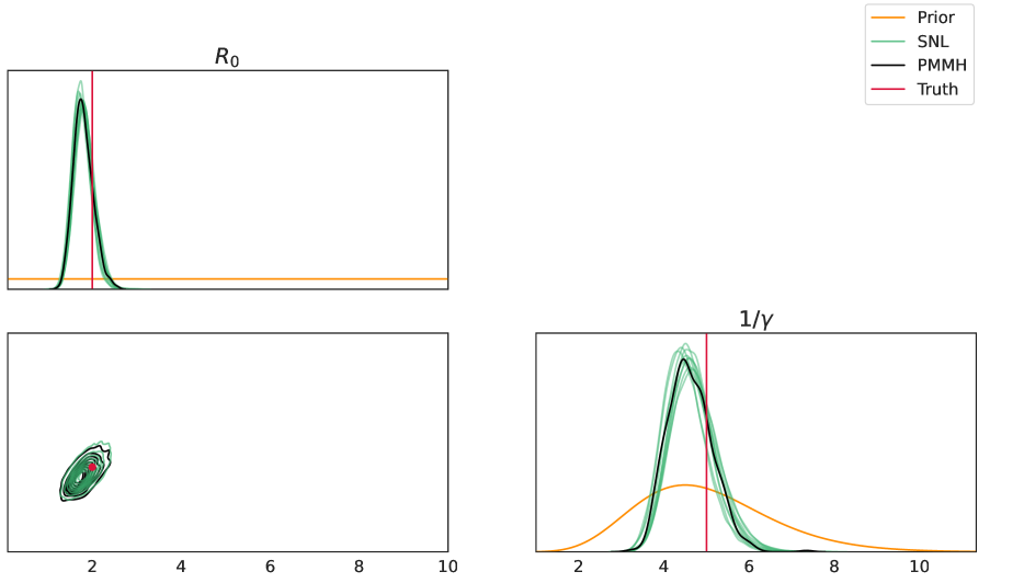
Figure 6: Posterior pairs plot for observed data from the SIR model across 100 households.

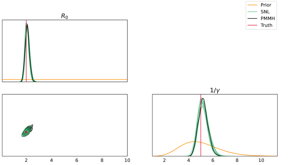
Figure 7: Posterior pairs plot for observed data from the SIR model across 200 households.

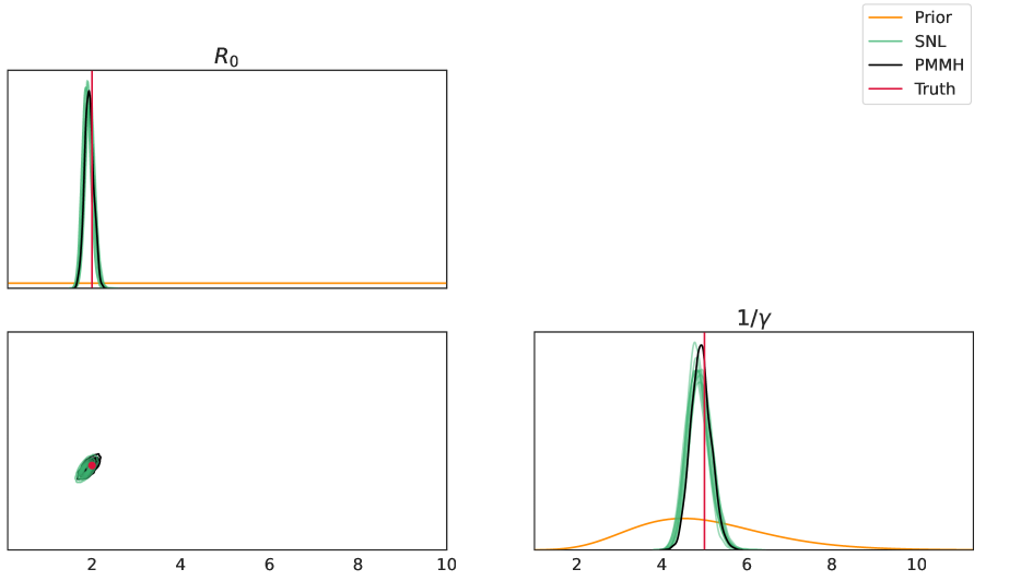
Figure 8: Posterior pairs plot for observed data from the SIR model across 500 households.

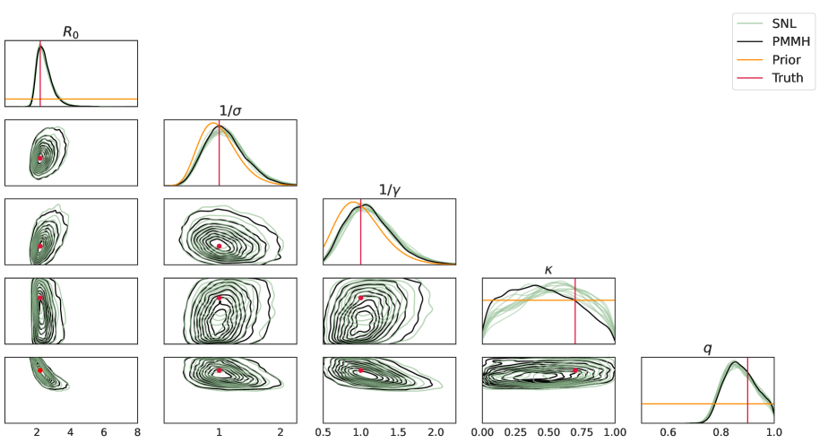
Figure 9: Posterior pairs plot for observed outbreak from SEIAR model with population size $N=350$.

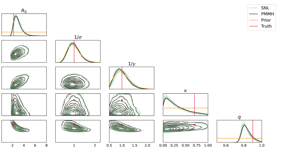
Figure 10: Posterior pairs plot for observed outbreak from SEIAR model with population size $N=500$.

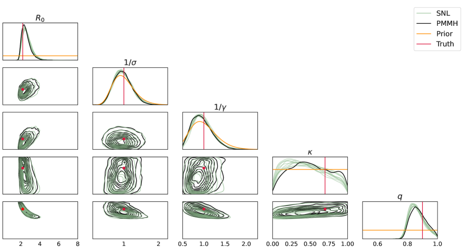
Figure 11: Posterior pairs plot for observed outbreak from SEIAR model with population size $N=1000$.

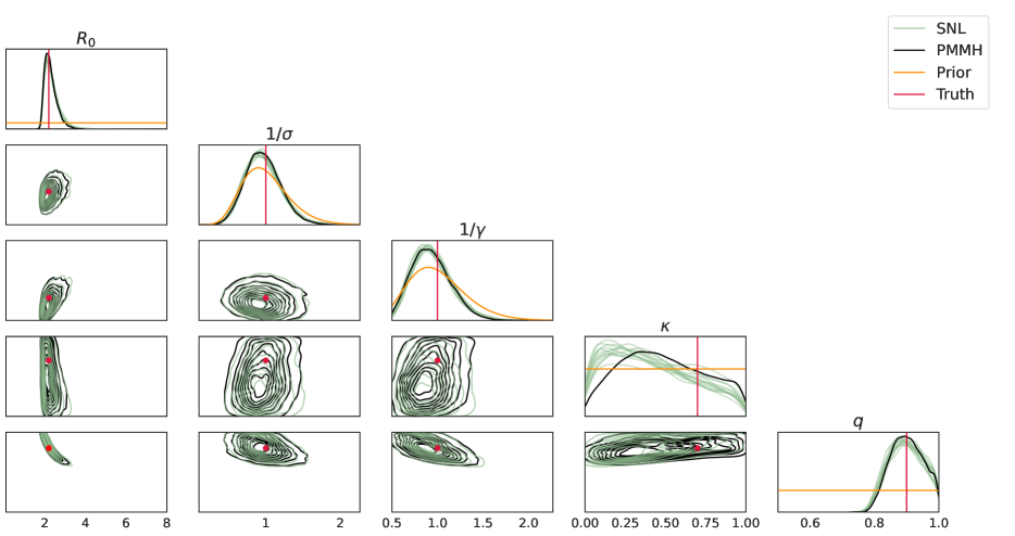
Figure 12: Posterior pairs plot for observed outbreak from SEIAR model with population size $N=2000$.

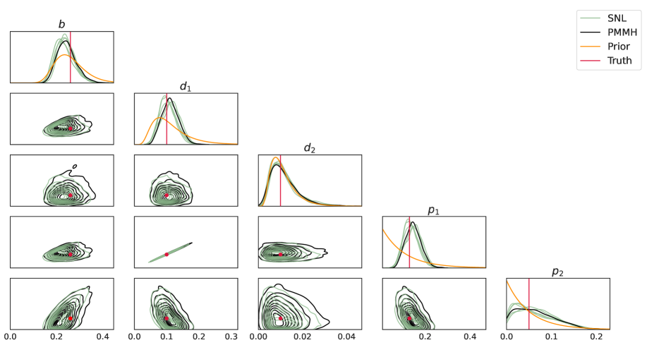
Figure 13: Posterior pairs plot for predator prey experiments with $r=0.5$.

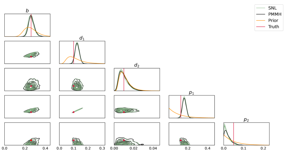
Figure 14: Posterior pairs plot for predator prey experiments with $r=0.7$.

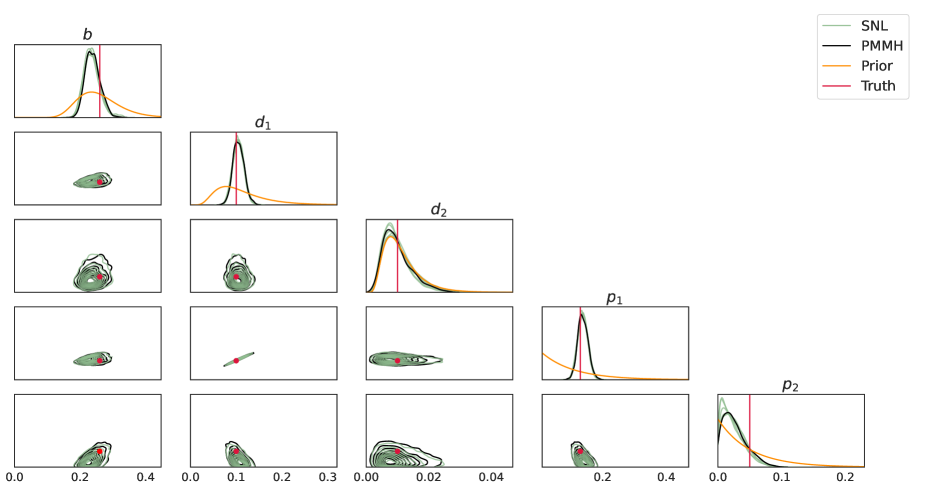
Figure 15: Posterior pairs plot for predator prey experiments with $r=0.9$.

References

- Allen (2017) L. J. Allen. A primer on stochastic epidemic models: Formulation, numerical simulation, and analysis. Infectious Disease Modelling, 2:128–142, 2017. doi: 10.1016/j.idm.2017.03.001.
- Andrieu and Roberts (2009) C. Andrieu and G. O. Roberts. The pseudo-marginal approach for efficient Monte Carlo computations. The Annals of Statistics, 37:697–725, 2009. doi: 10.1214/07-AOS574.
- Andrieu et al. (2010) C. Andrieu, A. Doucet, and R. Holenstein. Particle Markov chain Monte Carlo methods. Journal of the Royal Statistical Society: Series B (Statistical Methodology), 72(3):269–342, 2010. doi: 10.1111/j.1467-9868.2009.00736.x.
- Arnol’d and Gamkrelidze (1994) V. I. Arnol’d and R. V. Gamkrelidze. Dynamical Systems V: Bifurcation Theory and Catastrophe Theory. Springer, Berlin, 1994. doi: 10.1007/978-3-642-57884-7.
- Bardenet et al. (2017) R. Bardenet, A. Doucet, and C. Holmes. On Markov chain Monte Carlo methods for tall data. Journal of Machine Learning Research, 18:1–43, 2017.
- Bickel et al. (2008) P. Bickel, B. Li, and T. Bengtsson. Sharp failure rates for the bootstrap particle filter in high dimensions. In Institute of Mathematical Statistics Collections, pages 318–329. Institute of Mathematical Statistics, Beachwood, Ohio, 2008. doi: 10.1214/074921708000000228.
- Black (2019) A. J. Black. Importance sampling for partially observed temporal epidemic models. Statistics and Computing, 29:617–630, 2019. doi: 10.1007/s11222-018-9827-1.
- Black et al. (2017) A. J. Black, N. Geard, J. M. McCaw, J. McVernon, and J. V. Ross. Characterising pandemic severity and transmissibility from data collected during first few hundred studies. Epidemics, 19:61–73, 2017. doi: 10.1016/j.epidem.2017.01.004.
- Bradbury et al. (2018) J. Bradbury, R. Frostig, P. Hawkins, M. J. Johnson, C. Leary, D. Maclaurin, G. Necula, A. Paszke, J. VanderPlas, S. Wanderman-Milne, and Q. Zhang. JAX: composable transformations of Python+NumPy programs, 2018. URL http://github.com/google/jax.
- Breuer and Baum (2005) L. Breuer and D. Baum. An Introduction to Queueing Theory and Matrix-Analytic Methods. Springer-Verlag, 2005. doi: 10.1007/1-4020-3631-0.
- Brooks et al. (2011) S. Brooks, A. Gelman, G. Jones, and X.-L. Meng. Handbook of Markov Chain Monte Carlo. Chapman and Hall/CRC, first edition, 2011. doi: 10.1201/b10905.
- Chen et al. (2020) Y. Chen, Y. Kang, Y. Chen, and Z. Wang. Probabilistic forecasting with temporal convolutional neural network. Neurocomputing, 399:491–501, 2020. doi: 10.1016/j.neucom.2020.03.011.
- Chopin and Papaspiliopoulos (2020) N. Chopin and O. Papaspiliopoulos. An Introduction to Sequential Monte Carlo. Springer, 2020. doi: 10.1007/978-3-030-47845-2.
- Cranmer et al. (2020) K. Cranmer, J. Brehmer, and G. Louppe. The frontier of simulation-based inference. Proceedings of the National Academy of Sciences, 117(48):30055, 2020. doi: 10.1073/pnas.1912789117.
- Del Moral (2004) P. Del Moral. Feynman-Kac Formulae. Springer, New York, 2004. doi: 10.1007/978-1-4684-9393-1.
- Del Moral and Murray (2015) P. Del Moral and L. M. Murray. Sequential Monte Carlo with Highly Informative Observations. SIAM/ASA Journal on Uncertainty Quantification, 3:969–997, 2015. doi: 10.1137/15M1011214.
- Del Moral et al. (2015) P. Del Moral, P. Jasra, A. Lee, C. Yau, and X. Zhang. The alive particle filter and its use in particle Markov chain Monte Carlo. Stoch. Anal. Appl., 33:943–974, 2015.
- Doucet et al. (2015) A. Doucet, M. K. Pitt, G. Deligiannidis, and R. Kohn. Efficient implementation of Markov chain Monte Carlo when using an unbiased likelihood estimator. Biometrika, 102:295–313, 2015. doi: 10.1093/biomet/asu075.
- Drovandi and McCutchan (2016) C. C. Drovandi and R. A. McCutchan. Alive SMC2: Bayesian model selection for low-count time series models with intractable likelihoods. Biometrics, 72:344–353, 2016. doi: 10.1111/biom.12449.
- Germain et al. (2015) M. Germain, K. Gregor, I. Murray, and H. Larochelle. MADE: Masked Autoencoder for Distribution Estimation. In International Conference on Machine Learning, volume 37, pages 881–889, 2015.
- Gillespie (1976) D. T. Gillespie. A general method for numerically simulating the stochastic time evolution of coupled chemical reactions. Journal of Computational Physics, 22(4):403–434, 1976. doi: 10.1016/0021-9991(76)90041-3.
- Greenberg et al. (2019) D. Greenberg, M. Nonnenmacher, and J. Macke. Automatic Posterior Transformation for Likelihood-Free Inference. In International Conference on Machine Learning, volume 97, pages 2404–2414, 2019.
- He et al. (2016) K. He, X. Zhang, S. Ren, and J. Sun. Deep Residual Learning for Image Recognition. In IEEE Conference on Computer Vision and Pattern Recognition (CVPR), pages 770–778, 2016. doi: 10.1109/CVPR.2016.90.
- Hendrycks and Gimpel (2016) D. Hendrycks and K. Gimpel. Gaussian Error Linear Units (GELUs). arXiv preprint arXiv:1606.08415, 2016.
- Hermans et al. (2020) J. Hermans, V. Begy, and G. Louppe. Likelihood-free MCMC with amortized approximate ratio estimators. In International Conference on Machine Learning, volume 119, pages 4239–4248, 2020.
- Hermans et al. (2022) J. Hermans, A. Delaunoy, F. Rozet, A. Wehenkel, V. Begy, and G. Louppe. A Crisis In Simulation-Based Inference? Beware, Your Posterior Approximations Can Be Unfaithful. Transactions on Machine Learning Research, 2022.
- Hoffman and Gelman (2014) M. D. Hoffman and A. Gelman. The No-U-Turn Sampler: Adaptively Setting Path Lengths in Hamiltonian Monte Carlo. Journal of Machine Learning Research, 15(47):1593–1623, 2014.
- Karlin and Taylor (1975) S. Karlin and H. M. Taylor. A First Course in Stochastic Processes. Academic Press, second edition, 1975.
- Kitagawa (1996) G. Kitagawa. Monte Carlo Filter and Smoother for Non-Gaussian Nonlinear State Space Models. Journal of Computational and Graphical Statistics, 5:1–25, 1996. doi: 10.1080/10618600.1996.10474692.
- Kobyzev et al. (2021) I. Kobyzev, S. J. Prince, and M. A. Brubaker. Normalizing flows: An introduction and review of current methods. IEEE Transactions on Pattern Analysis and Machine Intelligence, 43(11):3964–3979, 2021. doi: 10.1109/TPAMI.2020.2992934.
- Loshchilov and Hutter (2017) I. Loshchilov and F. Hutter. Decoupled Weight Decay Regularization. arXiv preprint arXiv:1711.05101, 2017.
- McKane and Newman (2005) A. J. McKane and T. J. Newman. Predator-prey cycles from resonant amplification of demographic stochasticity. Phys. Rev. Lett., 94:218102, 2005. doi: 10.1103/PhysRevLett.94.218102.
- Neal (2011) R. Neal. MCMC Using Hamiltonian Dynamics. Chapman and Hall/CRC, first edition, 2011. doi: 10.1201/b10905.
- O’Neill and Roberts (1999) P. D. O’Neill and G. O. Roberts. Bayesian inference for partially observed stochastic epidemics. Journal of the Royal Statistical Society. Series A (Statistics in Society), 162(1):121–129, 1999.
- Papamakarios et al. (2019) G. Papamakarios, D. Sterratt, and I. Murray. Sequential Neural Likelihood: Fast Likelihood-free Inference with Autoregressive Flows. In Proceedings of Machine Learning Research, volume 89, pages 837–848, 2019.
- Phan et al. (2019) D. Phan, N. Pradhan, and M. Jankowiak. Composable Effects for Flexible and Accelerated Probabilistic Programming in NumPyro. arXiv preprint arXiv:1912.11554, 2019.
- Rasul et al. (2021) K. Rasul, A.-S. Sheikh, I. Schuster, U. M. Bergmann, and R. Vollgraf. Multivariate Probabilistic Time Series Forecasting via Conditioned Normalizing Flows. In International Conference on Learning Representations, 2021.
- Ross (2000) S. M. Ross. Introduction to Probability Models. Academic Press, 7th edition, 2000.
- Salimans et al. (2017) T. Salimans, A. Karpathy, X. Chen, and D. P. Kingma. PixelCNN++: A PixelCNN Implementation with Discretized Logistic Mixture Likelihood and Other Modifications. In International Conference on Learning Representations, 2017.
- Salinas et al. (2020) D. Salinas, V. Flunkert, J. Gasthaus, and T. Januschowski. DeepAR: Probabilistic forecasting with autoregressive recurrent networks. International Journal of Forecasting, 36(3):1181–1191, 2020. doi: 10.1016/j.ijforecast.2019.07.001.
- Shea and Ackers (1985) M. A. Shea and G. K. Ackers. The OR control system of bacteriophage lambda. Journal of Molecular Biology, 181:211–230, 1985. doi: 10.1016/0022-2836(85)90086-5.
- Sherlock (2021) C. Sherlock. Direct statistical inference for finite Markov jump processes via the matrix exponential. Computational Statistics, 36:2863–2887, 2021. doi: 10.1007/s00180-021-01102-6.
- Sherlock et al. (2015) C. Sherlock, A. H. Thiery, G. O. Roberts, and J. S. Rosenthal. On the efficiency of pseudo-marginal random walk metropolis algorithms. Ann. Stats., 43:238–275, 2015.
- Shumway and Stoffer (2017) R. H. Shumway and D. S. Stoffer. Time Series Analysis and Its Applications: With R Examples. Springer, 2017. doi: 10.1007/978-3-319-52452-8.
- Snyder (2012) C. Snyder. Particle filters, the optimal proposal and high-dimensional systems. PhD Thesis, ECMWF, Shinfield Park, Reading, 2012.
- van den Oord et al. (2016) A. van den Oord, S. Dieleman, H. Zen, K. Simonyan, O. Vinyals, A. Graves, N. Kalchbrenner, A. Senior, and K. Kavukcuoglu. WaveNet: A Generative Model for Raw Audio. arXiv preprint arXiv:1609.03499, 2016.
- van Kampen (1992) N. G. van Kampen. Stochastic processes in physics and chemistry. Elsevier, Amsterdam, 1992.
- Vaswani et al. (2017) A. Vaswani, N. Shazeer, N. Parmar, J. Uszkoreit, L. Jones, A. N. Gomez, L. Kaiser, and I. Polosukhin. Attention is All You Need. In Advances in Nerual Information Processing Systems, pages 6000–6010, 2017.
- Walker et al. (2017) J. N. Walker, J. V. Ross, and A. J. Black. Inference of epidemiological parameters from household stratified data. PLoS ONE, 12:e0185910, 2017. doi: 10.1371/journal.pone.0185910.
- Wilkinson (2018) D. J. Wilkinson. Stochastic Modelling for Systems Biology, Third Edition. Chapman and Hall/CRC, third edition, 2018. doi: 10.1201/9781351000918.