WeaveNet for Approximating Two-sided Matching Problems

Abstract

Matching, a task to optimally assign limited resources under constraints, is a fundamental technology for society. The task potentially has various objectives, conditions, and constraints; however, the efficient neural network architecture for matching is underexplored. This paper proposes a novel graph neural network (GNN), WeaveNet, designed for bipartite graphs. Since a bipartite graph is generally dense, general GNN architectures lose node-wise information by over-smoothing when deeply stacked. Such a phenomenon is undesirable for solving matching problems. WeaveNet avoids it by preserving edge-wise information while passing messages densely to reach a better solution. To evaluate the model, we approximated one of the strongly NP-hard problems, fair stable matching. Despite its inherent difficulties and the network’s general purpose design, our model reached a comparative performance with state-of-the-art algorithms specially designed for stable matching for small numbers of agents.

1 Introduction

From job matching to multiple object tracking (MOT), matching problems can represent various decision-making applications. A matching problem is generally described on a bipartite graph, a graph that has two sets of nodes $A$ and $B$ with edges $E=A\times B$ ($N=|A|$, $M=|B|$, $N\geq M$). On the graph, the task is to find a matching $m$ (a set of edges that do not share any nodes) that maximally satisfies an objective. The most famous objective is to maximize the sum of edge weights in $m$, which can be solved by the Hungarian algorithm Kuhn (1955). This problem is called one-sided because only one stakeholder dominates both sides $A$ and $B$. In contrast, two-sided matching supposes that agents on each side aim to maximize their reward.

A fairer two-sided matching solver provides more agreeable social decisions, but some fairness objectives make the problem strongly NP-hard Kato (1993); McDermid and Irving (2014). Besides, agents may randomly appear/disappear in dynamic matching problems (e.g., MOT with occlusions Emami et al. (2020)). In such cases, we need to compensate for the inputs of incomplete information by its stochastic properties. A learning-based model can be an alternative to hand-crafted algorithms for such applications. However, such models are underexplored.

This paper aims to propose an effective learning-based solver for matching problems and evaluate it on strongly NP-hard conditions of fair stable matching problems.

The contribution of this paper is four-fold:

1. We proposed WeaveNet, a novel neural network architecture for matching problems that largely outperforms traditional learning-based approaches.

2. For the first time, our learning-based solver achieved a comparative performance to the state-of-the-art handcrafted algorithm of NP-hard matching problems, though it was achieved with the limited size of problem instances ($N=20,~{}30$).

3. For the first time, we demonstrated the performance of a deep model unsupervisedly trained by a continuous relaxation of discrete conditions of matching problems.

4. We provided a steady baseline for the problem with source code to open a new vista for learning-based combinatorial optimization.

2 Background and Related Work

2.1 Stable Matching Problem

In this study, we evaluate our model with a typical two-sided problem of stable matching. An instance $I$ of a stable matching problem consists of two sets of agents $A$ and $B$ on a bipartite graph. Fig. 1 illustrates an example of $I$. Each agent $a_{i}$ in $A~{}(0<i\leq N)$ has a preference list $p^{A}_{i}$, which is an ordered set of elements in $B$ and $p^{A}_{ij}=rank(b_{j};p^{A}_{i})$ is the index of $b_{j}$ in the list $p^{A}_{i}$. $a_{i}$ prefers $b_{j}$ to $b_{j^{\prime}}$ if $p^{A}_{ij}<p^{A}_{ij^{\prime}}$. Similarly, each agent $b_{j}$ in $B(0<j\leq M)$ has a preference list $p_{j}^{B}$.

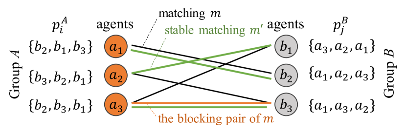
Figure 1: An example of a stable matching instance with a size of $N=3$. The matching $m$ (black edges) is not stable due to the blocking pair (the orange edge). The matching $m^{\prime}$ (green edges) is a stable matching.

For a matching $m\in\{0,1\}^{N\times M}$, we say that an unmatched pair $\{a_{v},b_{w}\}(\notin m)$ blocks $m$ if there are matched pairs $\{a_{v},b_{j}\}\in m$ and $\{a_{i},b_{w}\}\in m$ that satisfy $p^{A}_{vw}<p^{A}_{vj}$ and $p^{B}_{wv}<p^{B}_{wi}$. Here, $\{a_{v},b_{w}\}$ is called a blocking pair (the orange edge blocks a matching of black edges in the figure).

A matching is called stable if it has no blocking pair (the green edges in the figure). It is known that an instance $I$ always has at least one stable matching, and the Gale-Shapley (GS) algorithm can find it in $O(N^{2})$ Gale and Shapley (1962). However, the algorithm prioritizes either side and the other side only gets the least preferable result among all the possibilities of stable matching.

Cost	Definition
Sex equality	$SEq(m;I)$	$\!=\!$	$|P(m;A)-P(m;B)|$
Regret	$Reg(m;I)$	$\!=\!$	$\max_{\{a_{i},b_{j}\}\in m}(\max(p^{A}_{ij},p^{B}_{ji}))$
Egalitarian	$Egal(m;I)$	$\!=\!$	$P(m;A)+P(m;B)$
Balance	$Bal(m;I)$	$\!=\!$	$\max(P(m;A),P(m;B))$

Table 1: Representative costs to measure the fairness of matching.

To compensate for the unfairness, there have been diverse measures of fairness proposed, with different complexities of finding an optimal solution. They are listed in Table 1 with the definitions, where

$$P(m;A)=\!\!\sum_{\{a_{i},b_{j}\}\in m}\!\!p^{A}_{ij}, P(m;B)=\!\!\sum_{\{a_{i},b_{j}\}\in m}\!\!p^{B}_{ji}.$$ (1)

Sex equality cost ($SEq$) is a popular measure that focuses on the unfairness brought by the gap between the two sides’ satisfaction Gusfield and Irving (1989). Regret cost ($Reg$) measures the unfairness brought by the agent who obtained the least satisfaction (the weakest individual) in the matching. Egalitarian cost ($Egal$) measures the overall satisfaction, in other words, the greater good, rather than concerning the weaker individual or weaker side Gusfield and Irving (1989). Balance cost ($Bal$) is a compromise between side-equality and overall satisfaction Feder (1995); Gupta et al. (2019), and equivalent to $\frac{1}{2}(SEq+Egal)$. Minimizing balance cost is to benefit the weaker side while less harming the stronger side.

Among these measures, a stable matching of minimum regret cost and minimum egalitarian cost can be found in $O(N^{2})$ and $O(N^{3})$, respectively Gusfield (1987); Irving et al. (1987); Feder (1992), while minimizing sex equality cost or balance cost is known as strongly NP-hard Kato (1993); McDermid and Irving (2014); Feder (1995).

There are several approximation solvers for the strongly NP-hard stable matching variants. Iwama et al. proposed a method that runs in $O(N^{3+\frac{1}{\varepsilon}})$ whose gap from the optimal solution is bounded by $\varepsilon$ Iwama et al. (2010). Deferred Acceptance with Compensation Chains (DACC) is an extension of the GS algorithm without prioritizing any side. It can terminate in $O(N^{4})$ Dworczak (2016). PowerBalance is a state-of-the-art algorithm. In each round of proposing, it balances the two sides by letting the stronger side propose (because their satisfactions decrease if getting rejected). It was reported that PowerBalance has competitive performance when enforcing a termination in $O(N^{2})$ Tziavelis et al. (2019).

2.2 Learning-based Matching Solvers

Although learning-based matching solvers are still in the process of development, it has potential applications when we can only observe incomplete information. The dynamic matching problem Wang et al. (2019) is one typical case. Another case is temporal alignment, where we have only superficial observation (videos, audio, or narration) and cannot access the true similarity between temporal events. Learning-based solvers would be helpful to jointly train the feature encoder with the matching module Fathony et al. (2018).

Learning-based solvers also have advantages in flexibility even to deal with variations of traditional matching problems (e.g., incomplete preference lists with ties, continuous preference scores, or multi-dimensional preference Chen et al. (2018)) as well as more complex objective functions (e.g., a weighted sum of costs in Table 1). Aiming to develop learning-based methods for the stable matching problem, Li (2019) proposed a loss function that relaxes the discrete constraints on matching stability into a continuous measure, which enables to train a model in an unsupervised manner. However, they only provide an experiment on $N=5$ with a shallow neural network.

Deep Bipartite Matching (DBM) Gibbons et al. (2019) is another attempt to approximate the (not strongly) NP-hard problem of weapon-target assignment (WTA), but its performance is not at a comparative level with the state-of-the-art of WTA approximation Ahuja et al. (2007) even limiting the size of problem instances.

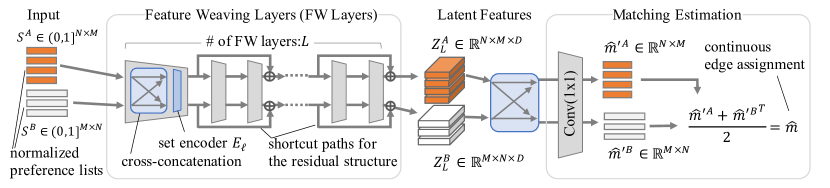
Figure 2: WeaveNet architecture. $L$ feature weaving layers are stacked with shortcut paths to be a deep network. The encoded features are fed into Conv(1$\times$1) layer to obtain logits ($\hat{m}^{\prime A}$, $\hat{m}^{\prime B}$). The output $\hat{m}$ will be binarized in prediction phase to represent a matching.

3 Deep-learning-based Fair Stable Matching

3.1 WeaveNet

3.1.1 Input and Output Data Format

We aim to realize a trainable function $F$ that outputs a matching $\hat{m}$, which is an $N\times M$ matrix. As for the input, we firstly linearly re-scale the rank of preference $p^{*}_{ij}~{}(*\in\{A,B\})$ ranged in $[1,N]$ into a normalized score $s^{*}_{ij}$ ranged in $(0,1]$ to make it invariant to $N$, where 1 for the highest rank. Then, we obtain the input as matrices $S^{A}$ and $S^{B}$, where $s^{A}_{ij}$ is the $ij$-element of $S^{A}$.

3.1.2 Requirement, Intuition and Entire Model

One of the required properties of $F:(S^{A},~{}S^{B})\rightarrow\hat{m}$ is to take all the agents’ preference into account when determining the presence of each edge in the output $\hat{m}$. Li (2019) implemented this by multilayer perceptron (MLP), where $S^{A}$ and $S^{B}$ are destructured and concatenated into a flat vector (with the length of $2NM$) and fed to the MLP. Its output (a flat vector with the length of $NM$) is restructured into a matrix $\hat{m}\in{\mathcal{R}}^{N\times M}$. The MLP model, however, would face difficulties due to the following four problems.

(a)

Preference lists of multiple agents are encoded by independent parameters, though they share a format so that we could efficiently process them in the same manner.

(b)

MLP only supports a fixed-size input, so training different models for different cases of $N$ becomes mandatory.

(c)

$F$ should be permutation invariant, which means the matching result unchanged even if we shuffle the order of agents in $S^{A}$ and $S^{B}$, but MLP does not satisfy.

(d)

A shallow MLP model may be insufficient to approximate an exact solver for the NP-hard problem when $N$ is large.

To address the above weaknesses of MLP, we propose the feature weaving network (WeaveNet) which has the properties of (a) shared encoder, (b) variable-size input, (c) permutation invariance, and (d) residual structure. The WeaveNet, as shown in Fig. 2, consists of $L$ feature weaving (FW) layers. It has two streams of $A$ and $B$. In a symmetric manner, each stream models the agent’s act of selecting the one on the opposite side while sharing weights to enhance the parameter efficiency. The shortcut paths at every two FW layers make them residual blocks, which allows the model to be as deep as possible. We explain its details as follows.

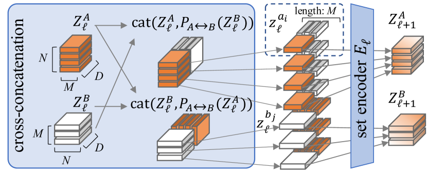
Figure 3: Feature weaving layer orthogonally concatenates the weftwise and warpwize components ($Z_{\ell}^{A}$ and $Z_{\ell}^{B}$) in a symmetric way (cross-concatenation). Then, the concatenated tensors are separated into $z_{\ell}^{\smash{a_{i}}}$ (or $z_{\ell}^{\smash{b_{j}}}$), which represents a set of outgoing edges from agent $a_{i}$ (or $b_{j}$), and independently fed to $E_{\ell}$.

3.1.3 Feature Weaving Layer

Fig. 3 illustrates the detail of a single FW layer, which is the core architecture of the proposed network. FW layer is a two-stream layer whose inputs consist of a weftwise component $Z^{A}_{\ell}$ and a warpwise component $Z^{B}_{\ell}$, where $Z^{A}_{0}=S^{A}$ and $Z^{B}_{0}=S^{B}$. The two components are symmetrically concatenated in each stream (cross-concatenation). Then these concatenations are separated into agent-wise features, each of which is a set of outgoing-edge features of an agent (indicating the preference from that agent to every matching candidate). These features are processed by the encoder $E_{\ell}$ shared by every agent in both $A$ and $B$. As for an encoder that can embed variable-size input in a permutation invariant manner, we adopted the structure proposed in DeepSet Zaheer et al. (2017) and PointNet Qi et al. (2017), which consists of two convolutional layers with kernel size $1$ and a set-wise max-pooling layer, followed by batch-normalization and activation. We refer to this structure as set encoder. See A.2 for visualization of the set encoder and its calculation cost.

3.1.4 Difference from DBM

Note that DBM Gibbons et al. (2019) also satisfies the requirements (b), (c), and (d). The critical difference between WeaveNet and DBM is its parameter efficiency and the choice of the local structure $E_{\ell}$. DBM applies the weftwise and warpwise communications alternately in a single-stream architecture. Hence, each encoder is specialized in each direction. In our model, every encoder is trained for both directions, and thus it is twice parameter efficient. See A.3 to know how WeaveNet and DBM propagate the weftwise and warpwise communications. Also, the local structure of DBM is sub-optimal to encode the relative identity of each outgoing edge among $N\times M$ pairs. We show the difference in performance brought by the local structure $E_{\ell}$ in the experiment section.

3.1.5 Mathematical Formulations of WeaveNet

The input $Z^{A}_{\ell}$ is a third-order tensor whose dimensions, in sequence, corresponding to the agent, candidate, and feature dimension, with a size of $(N,M,D)$. Similarly, $Z^{B}_{\ell}$ has a size of $(M,N,D)$. The cross-concatenation is defined by function $P_{A\leftrightarrow B}$, which swaps the first and second dimensions of the tensor, and $cat(\{Z_{1},Z_{2},\ldots\})$, which concatenates the features of two tensors $Z_{1},~{}Z_{2}$, as

$$\begin{split}Z^{\prime A}_{\ell}&=cat(Z^{A}_{\ell},P_{A\leftrightarrow B}(Z^{B}_{\ell})).\end{split}$$ (2)

$Z^{\prime A}_{\ell}$ is sliced into agent-wise features $z^{a_{i}}_{\ell}$ and we obtain $Z^{A}_{\ell+1}=(E_{\ell}(z^{a_{i}}_{\ell})|0<i\leq N)$. We can calculate $Z^{B}_{\ell+1}$ in a symmetric manner (with the same encoder $E_{\ell}$).

After the process of $L$ FW layers, $Z^{A}_{L}$ and $Z^{B}_{L}$ are further cross-concatenated and fed to the matching estimator (in Fig. 2). It outputs a non-deterministic matching $\hat{m}$. In the training phase, $\hat{m}$ is input to an objective function, and the loss is minimized. In the prediction phase, the matching is obtained by binarizing $\hat{m}$. In this sense, matching estimation through a neural network can be considered as an approximation by relaxing the binary matching space $\{0,1\}^{N\times M}$ (where 1 represents the edge selection while 0 for rejection) into a continuous matching space $[0,1]^{N\times M}$.

3.1.6 Symmetric Property and Asymmetric Variant

WeaveNet is designed to be fully symmetric for $S^{A}$ and $S^{B}$. Hence, it satisfies the equation $F(S^{A},S^{B})=F(S^{B},S^{A})^{\top}$. This condition ensures that the model architecture cannot distinguish the two sides $A$ and $B$ innately. This property is beneficial when mathematically fair treatment between $A$ and $B$ is desirable. However, when inputs from $A$ and $B$ are differently biased (e.g., the two sides have different trends of preference), sharing encoders in two directions may degrade the performance. To eliminate the bias difference without losing the parameter-efficiency, we further propose to a) apply batch normalization independently for each stream, and b) adding a side-identifiable code (e.g., 1 for $A$ and 0 for $B$) to $Z^{A}_{0}$ and $Z^{B}_{0}$ as a ($D$+1)-th element of the feature. We call this variant “asymmetric”.

3.2 Relaxed Continuous Optimization

Generally, a combinatorial optimization problem has discrete objective functions and conditions, which are not differentiable. To optimize the model in an end-to-end manner without inaccessible ground truth, we optimize the model by relaxing such discrete loss functions into continuous ones.

Assume we target to obtain a fair stable matching that has the minimum $SEq$, for example. Then, we have the following three loss functions.

${\mathcal{L}}_{m}$

conditions the binarization of $\hat{m}$ to represent a matching.

${\mathcal{L}}_{s}$

conditions the matching to be stable.

${\mathcal{L}}_{f}$

minimizing the fairness cost $SEq$ of the matching

The overall loss function is defined as

$${\mathcal{L}}_{\rm fsm}(\hat{m}) =\lambda_{m}{\mathcal{L}}_{m}+\frac{1}{2}\sum_{m\in\{\hat{m}^{A},\hat{m}^{B}\}}\bigl{(}\lambda_{s}{\mathcal{L}}_{s}(m)+\lambda_{f}{\mathcal{L}}_{f}(m)\bigr{)},$$ (3)

where $\hat{m}^{A}={\rm softmax}(\hat{m})$ and $\hat{m}^{B}={\rm softmax}(\hat{m}^{\top})$.

An advantage of learning-based approximation is its flexibility. We can modify the above loss functions to easily obtain other variants. For example, removing ${\mathcal{L}}_{f}$ in Eq.(3) leads to standard stable matching, and replacing ${\mathcal{L}}_{f}$ with ${\mathcal{L}}_{b}$ (which minimizes $Bal$) leads to balanced fair-stable matching, as follows:

$${\mathcal{L}}_{\rm sm}(\hat{m}) =\lambda_{m}{\mathcal{L}}_{m}+\frac{1}{2}\sum_{m\in\{\hat{m}^{A},\hat{m}^{B}\}}\lambda_{s}{\mathcal{L}}_{s}(m),$$ (4)

$${\mathcal{L}}_{\rm bsm}(\hat{m}) =\lambda_{m}{\mathcal{L}}_{m}+\frac{1}{2}\sum_{m\in\{\hat{m}^{A},\hat{m}^{B}\}}\bigl{(}\lambda_{s}{\mathcal{L}}_{s}(m)+\lambda_{b}{\mathcal{L}}_{b}(m)\bigr{)}.$$ (5)

3.2.1 Matrix Constraint Loss ${\mathcal{L}}_{m}$

$\hat{m}$ can be safely converted into a binarized matching by column-wise or row-wise ${\rm argmax}$ operation when it is a symmetric doubly stochastic matrix Li (2019). To satisfy this condition, we defined ${\mathcal{L}}_{m}$ with an average of the cosine distance as

$$\begin{split}{\rm C}(\hat{m}^{A},\hat{m}^{B})&=\frac{1}{N}\sum_{i=0}^{N}\frac{\hat{m}^{A}_{i*}\cdot\hat{m}^{B}_{*i}}{\|\hat{m}^{A}_{i*}\|_{2}\|\hat{m}^{B}_{*i}\|_{2}}\\ {\mathcal{L}}_{m}(\hat{m}^{A},\hat{m}^{B})&=1-\frac{({\rm C}(\hat{m}^{A},\hat{m}^{B})+{\rm C}(\hat{m}^{B},\hat{m}^{A}))}{2},\end{split}$$ (6)

where $\hat{m}^{A}_{i*}$ means the $i$-th row of $\hat{m}^{A}$. This formulation binds $\hat{m}$ to be a symmetric doubly stochastic matrix when ${\mathcal{L}}_{m}(\hat{m}^{A},\hat{m}^{B})=0$. The advantage of this implementation against the original one in Li (2019) is described in B.1.

3.2.2 Blocking Pair Suppression by ${\mathcal{L}}_{s}$

As for $L_{s}$, we used the function proposed in Li (2019) as it is, which is

$$\begin{split}g(a_{i};b_{w},\hat{m})&=\sum_{b_{j}\neq b_{w}}\hat{m}_{ij}\cdot\max(S^{A}_{iw}-S^{A}_{ij},0)\\ g(b_{j};a_{v},\hat{m})&=\sum_{a_{i}\neq a_{v}}\hat{m}^{\top}_{ji}\cdot\max(S^{B}_{jv}-S^{B}_{ji},0)\\ {\mathcal{L}}_{s}(\hat{m};I)&=\sum_{(v,w)\in A\times B}g(a_{v};b_{w},\hat{m})g(b_{w};a_{v},\hat{m}),\end{split}$$ (7)

where $g(a_{i};b_{w},\hat{m})$ is a criterion known as ex-ante justified envy, which has a positive value when $a_{i}$ prefers $b_{w}$ more than any $b_{j}$ in $\{b_{j}|j\neq w,\hat{m}_{ij}>0\}$. This is the same for $g(b_{j};a_{v},\hat{m})$. Hence, $\{a_{v},b_{w}\}$ becomes a (soft) blocking pair when both $g(a_{v};b_{w},\hat{m})$ and $g(b_{w};a_{v},\hat{m})$ are positive.

3.2.3 ${\mathcal{L}}_{f}$ and ${\mathcal{L}}_{b}$ as Fairness Measurements

${\mathcal{L}}_{f}$, ${\mathcal{L}}_{b}$ minimize $SEq(m;I)$, $Bal(m;I)$ in Table 1, respectively, and are defined as

$${\mathcal{L}}_{f}(\hat{m};I) =\frac{1}{N}|S(\hat{m};A)-S(\hat{m};B)|,$$ (8)

$${\mathcal{L}}_{b}(\hat{m};I) =-\frac{1}{N}{\rm min}(S(\hat{m};A),S(\hat{m};B)),$$ (9)

where

$$~{}S(\hat{m};A)=\sum_{i=1}^{N}\sum_{i=j}^{M}\hat{m}_{ij}\cdot{S^{A}_{ij}},~{}S(\hat{m};B)=\sum_{j=1}^{M}\sum_{i=1}^{N}\hat{m}_{ij}\cdot{S^{B}_{ji}}.$$ (10)

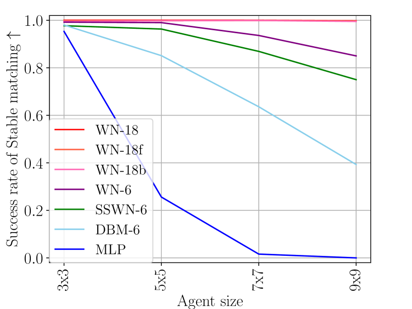
Figure 4: Change in the success rates of stable matching ($\uparrow$) according to $N$. 

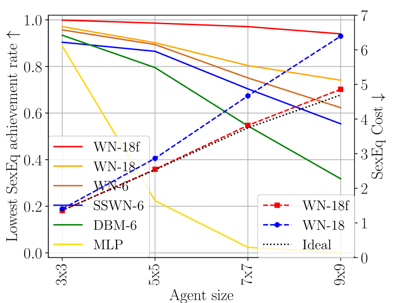
Figure 5: The rates of achieving the ideal fair-stable matching with minimum $SEq$ (solid, $\uparrow$), and the average $SEq$ (dashed, $\downarrow$).

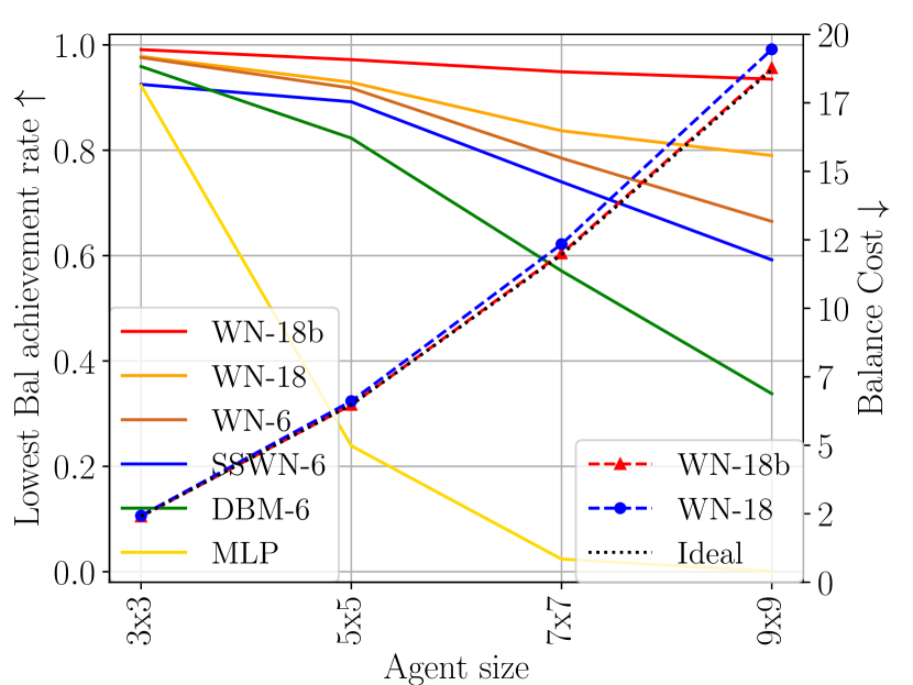
Figure 6: The rates of achieving the ideal fair-stable matching with minimum $Bal$ (solid, $\uparrow$), and the average $Bal$ (dashed, $\downarrow$).

4 Experiments

We evaluated WeaveNet through two experiments and one demonstration. First, with test samples of $N<10$, we compared its performance with learning-based baselines and optimal solutions obtained by a brute-force search. Second, we compared WeaveNet with algorithmic baselines at $N=20,~{}30$. Third, we demonstrate its performance at $N=100$. Note that we always assume $M=N$ hereafter.

4.0.1 Sample Generation Protocol

In the experiments, we used the same method as Tziavelis et al. (2019) to generate synthetic datasets that draw preference lists from the following distributions.

Uniform (U)

Each agent’s preference towards any matching candidate is totally random, defined by a uniform distribution $\mathcal{U}(0,1)$ (larger value means prior in the preference list).

Discrete (D)

Each agent has a preference of $\mathcal{U}(0.5,1)$ towards a certain group of $\lfloor 0.4N\rfloor$ popular candidates, while $\mathcal{U}(0,0.5)$ towards the rest.

Gauss (G)

Each agent’s preference towards $i$-th candidate is defined by a Gaussian distribution $\mathcal{N}(i/N,0.4)$.

LibimSeTi (Lib)

Simulate real rating activity on the online dating service LibimSeTi Brozovsky and Petricek (2007) based on the 2D distribution of frequency of each rating pair ($p^{A}_{ij},~{}p^{B}_{ji}$).

Choosing the above preference distributions for group $A$ and $B$ respectively, we obtained five different dataset settings, namely UU, DD, GG, UD, and Lib. We randomly generated 1,000 test samples and 1,000 validation samples for each of the five distribution settings.

4.0.2 Training Protocol

We trained any learning-based models 200k total iterations at $N\leq 30$ and 300k at $N=100$, with a batch size of $8$. We randomly generated training samples at each iteration based on the distribution of each dataset and used the Adam optimizer Kingma and Ba (2015). We set learning rate 0.0001 and loss weights $\lambda_{s}=0.7$, $\lambda_{m}=1.0$, $\lambda_{f}=\lambda_{b}=0.01$ based on a preliminary experiment (see A.4).

4.1 Comparison with Learning-based Methods

In this experiment, we show results obtained by following baselines and WeaveNet variants. MLP is the model proposed in Li (2019). DBM-6 is Deep Bipartite Matching Gibbons et al. (2019) with $L=6$ layers. SSWN-6 is the single-stream WeaveNet with $L=6$ layers. This variant is to test how WeaveNet works when adopting the single-stream design of DBM. WN-6 and WN-18 is the standard WeaveNet with $L=6$ and $L=18$ layers, respectively. All the above models were trained to optimize Eq. (4). WN-18f and WN-18b have the same architecture with WN-18, but were trained to optimize Eq. (3) and Eq. (5), respectively. Note that MLP was trained for each $N$ because the network cannot flexibly accept different-size problem instances. The other methods were trained with samples of $N=10$ and tested on samples of $N=3,~{}5,~{}7,~{}9$. Models with $L=6$ have a similar number of parameters with the MLP model (for sample size $N=5$), so they can have a fair comparison of parameter efficiency. WN models with $L=18$ are aimed to show a larger potential. See B.1 for more precise definition of each architecture.

Fig. 6 shows the success rates of finding a stable matching. MLP can hardly find stable matchings when $N\geq 5$. DBM performs better than MLP but still obviously worse than any of WeaveNet variants. Standard WeaveNet’s two-stream architecture shows advantages over its single-stream variant.

Fig. 6 and 6 show the success rates of finding the possibly fairest (i.e., lowest $SEq$ or $Bal$) stable matching (solid lines) and the average costs of $SEq$ and $Bal$ (dashed lines), respectively. Each method has the same trend of performance as in Fig. 6. Specifically, the gap between WN-18 and WN-18f/b proved the flexibility of the model for customizing the objective function.

Agents ($N\times M$)	$20\times 20$					$30\times 30$
Datasets (Distribution Type)	UU	DD	GG	UD	Lib	UU	DD	GG	UD	Lib
GS	41.89	18.81	19.52	70.97	19.66	94.03	43.46	36.56	163.77	39.78
PolyMin	19.93	11.83	20.57	87.08	18.47	35.52	21.21	37.37	209.62	31.85
DACC	24.34	20.13	23.07	101.75	20.40	40.87	34.35	40.59	240.48	33.88
Power Balance	16.28	8.93	17.07	71.09	15.40	18.45	11.05	27.22	163.90	21.57
WN-60f (Ours)	11.44	6.32	15.34	71.18	14.44	16.07	9.64	26.46	162.61	21.29
Stable Match (%)	99.10	99.40	99.40	99.50	99.80	98.10	99.00	98.00	93.90	98.60
Win (%)	25.90	29.70	12.20	0.00	9.50	14.60	25.30	9.30	0.10	8.00
Tie (%)	67.30	60.60	83.20	96.70	86.20	72.30	54.70	78.10	89.20	80.80
Loss+Unstable (%)	6.80	9.70	4.60	3.30	4.30	13.10	20.00	12.60	10.70	11.20

Table 2: Average $SEq$ ($\downarrow$), success rate of stable matching, and winning/losing rate against the best algorithmic method (underlined).

Agents ($N\times M$)	$20\times 20$					$30\times 30$
Datasets (Distribution Type)	UU	DD	GG	UD	Lib	UU	DD	GG	UD	Lib
GS	89.14	146.16	108.36	140.53	68.62	184.05	322.05	225.49	312.12	137.59
PolyMin	74.19	140.99	108.04	145.28	66.94	144.48	306.28	224.13	324.54	130.79
DACC	78.49	146.71	110.06	151.34	68.75	150.71	316.18	227.52	337.43	133.59
Power Balance	73.28	140.12	106.92	140.55	65.89	138.04	302.30	220.26	312.12	126.96
WN-60b (Ours)	71.29	138.57	106.50	140.72	65.63	137.70	301.08	221.12	313.11	127.12
Stable Match (%)	98.00	99.10	98.60	99.80	99.10	97.00	98.60	93.70	98.80	98.00
Win (%)	20.60	29.80	9.40	0.00	6.60	10.40	25.70	6.20	0.10	5.60
Tie (%)	69.50	63.70	81.90	95.00	86.60	71.60	63.20	69.50	83.90	81.50
Loss+Unstable (%)	9.90	6.50	8.70	5.00	6.80	18.00	11.10	24.30	16.00	12.90

Table 3: Average $Bal$ ($\downarrow$), success rate of stable matching, and winning/losing rate against the best algorithmic method (underlined).

4.2 Comparison with Algorithmic Methods

GS is the better result of applying the GS algorithm Gale and Shapley (1962) to prioritize each side once. PolyMin is an algorithm that minimizes the regret and egalitarian costs (Table 1) instead of $SEq$ and $Bal$ costs, which we can calculate in polynomial time. DACC Dworczak (2016) is an approximate algorithm that runs in $O(n^{4})$. PowerBalance is the state-of-the-art method that runs in $O(n^{2})$.

WN-60f/b is WeaveNet with $L=60$ layers. It was trained with samples of $N=30$ and tested on $N=20,~{}30$. Note that we used the asymmetric variant for UD and Lib. See B.2 for a detailed ablation study for the symmetric and asymmetric variants and so on.

We show the results in Tables 3 and 3. In the $SEq$ experiment, the proposed WN-60f achieved the best scores almost in all the cases, and narrowly lost in UD for $N=20$. In the $Bal$ experiment, WN-60b also achieved the best scores in UU, DD, GG, and Lib for $N=20$ and UU, DD for $N=30$, and narrowly lost in the other four cases. Note that these scores of WN-60f/b involve unstable matchings.

To evaluate the results while strictly forbidding unstable matchings, we compared $SEq$ and $Bal$ obtained by WN-60f/b with the best algorithmic method (underlined in the table) sample by sample, and counted win, tie, and loss percentages of WN, where unstable matchings were treated as losses. Even with this setting, WN-60f beat the best algorithmic method in six among all the ten cases, and WN-60b won four among ten. To our best knowledge, other learning-based methods have never achieved such comparable results.

It is noteworthy that the asymmetric variant achieved a similar performance to the best algorithmic methods even in UD, the most biased setting, and Lib, the simulation of real preference distribution while keeping its parameter efficiency.

$100\times 100$, UU	$SEq$	$Bal$
GS	1259.39	1709.53
PolyMin	153.35	952.85
DACC	194.65	988.02
Power Balance	49.41	909.73
WN-80f/b+Hungarian	68.36	919.75
Stable Match (%)	89.4	80.8

Table 4: Average $SEq$ ($\downarrow$) and $Bal$ ($\downarrow$) at $N=100$.

4.3 Demonstration with $N=100$

We further demonstrate the capability of WeaveNet under relatively large size of problem instances, $N=100$. In this case, we found that the binarization process ${\rm argmax}(\hat{m})$ of WeaveNet does not always successfully yield a one-to-one matching. Specifically, WN-80f and WN-80b found stable matchings for 84.4% and 73.2% samples while failed to yield one-to-one matchings for 13.4% and 19.8%, respectively (see the Table 9 in B.2 for details). To compensate for this problem, we applied the Hungarian algorithm to $\hat{m}$ to force an output of one-to-one matching. The results in Table 4 demonstrate that WeaveNet still achieved a close performance to the state-of-the-art algorithmic method, under a problem size that other learning-based-method studies have never set foot into. We consider this result promising, and expect to further improve the scalability and the binarization reliability of WeaveNet.

5 Conclusion

This paper proposed a novel neural network architecture, WeaveNet, and evaluated it on fair stable matching, a strongly NP-hard problem. It outperformed any other learning-based methods by a large margin and achieved a comparative performance with the state-of-the-art algorithms under a limited size of problem instances. We hope that our proposed core module, the feature weaving layer, opens a new vista for machine learning and combinatorial optimization applications.

Appendix

Appendix A Further Implementation Details

A.1 Scaling Function

$p^{A}_{ij}$ has a value range of $[1,N]$, which depends on the size of the input problem instance. Moreover, general deep-learning frameworks (e.g., PyTorch and TensorFlow) initialize model weights under the assumption where the maximum value in the input data is around $1.0$. Hence, to re-scale $p^{A}_{ij}$ to $s^{A}_{ij}$, we used the following function $h$, which is

$$\begin{split}h(p^{A}_{ij})=((1-C_{min})(N-p^{A}_{ij}))/N+C_{min}\\ h(p^{B}_{ji})=((1-C_{min})(N-p^{B}_{ji}))/N+C_{min},\\ \end{split}$$ (11)

where $C_{min}$ should be a constant value in range $(0,1)$ and is set to 0.1 in our experiments.

A.2 Visualization of Set Encoder and Calculation Cost

The purpose of the set encoder is to embed the feature of an edge $a_{i}\rightarrow b_{j}$ while considering the relative relationship among the other out-edges from $a_{i}$. Because the number of out-edges is variable, the set encoder should also accept variable-size inputs. Besides, since the set of edges have no order, the encoder should output a permutation invariant result.

Such network structure is proposed in Zaheer et al. [2017] and Qi et al. [2017]. Following these studies, we implemented the encoder of WeaveNet as a structure that has two convolutional layers with a set-wise max-pooling layer. The pooling is done for each element in the feature vector and yields a single vector, which is then concatenated to each input feature. The illustration is in Fig. 7. In the experimental part, we refer to the number of output channels from the convolutional layers as $D^{\prime}$ and $D$, where $D^{\prime}$ is the intermediate feature fed to the max-pooling layer and $D$ is the output of this encoder. Following Qi et al. [2017], $D^{\prime}$ is typically set larger than $D$. Note that the structure is followed by the batch normalization and activation, for which we adopted the PReLU function.

A.2.1 Computational Complexity

With $D_{\max}=\max\{D^{\prime},D\}$, the theoretical calculation cost of a single set encoder on a single core processing unit is $O(N^{2}D_{\max}^{2})$, where a single linear operation in the convolution requires $D^{2}$ and we repeat it for $2N\times M$ elements ($N\geq M$). The other operations in WeaveNet, such as cross-concatenation, clearly have less cost. Hence, the entire WeaveNet has its calculation cost of $O(LN^{2}D_{\max}^{2})$.

We can reduce this into $O(L\log(ND_{\max}))$ with an ideal parallel processing unit. We have $2N\times M$ elements for the convolution and can linearly operate them independently. Each linear operation can be done in parallel except for weighted sum aggregation, which takes $O(\log(D_{\max}))$. Besides, we have a max-pooling operation, which consists of $D$ parallel max operations. It can also be done in parallel and each max operation for $N$ elements takes $O(\log N)$. Therefore, we can execute the calculation of a single set encoder in $O(\log(N)+\log(D_{\max}))$.

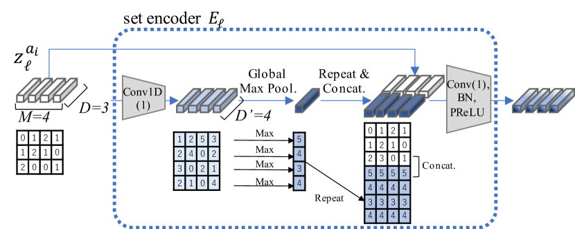
Figure 7: Illustration of the process in set encoder $E_{\ell}$, where $z_{\ell}^{a_{i}}$ (colored in white) is once encoded to $D^{\prime}$ channel features (colored in pale blue), then max-pooled to obtain statistics in the feature set (colored in blue). The statistics information is concatenated to each input feature and further encoded (color in a gradation).

A.3 Information Propagation with WeaveNet

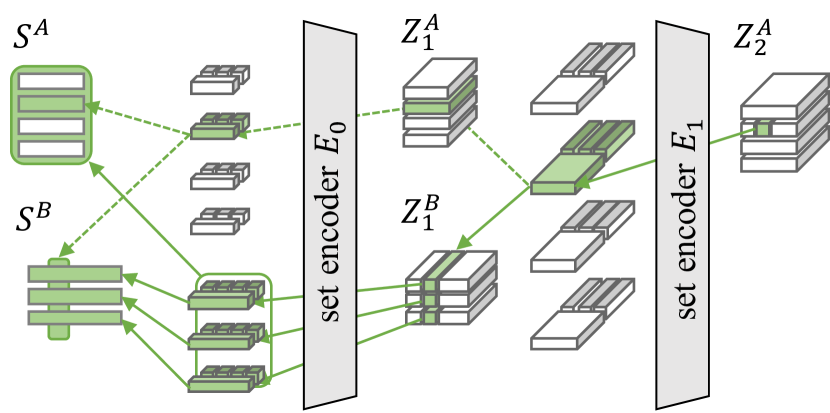
Figure 8: Backward path of WeaveNet (two-stream architecture) from $ij$-th feature in $Z^{A}_{2}$. The upper stream terminates at $i$-th row of $S^{A}$ and $i$-th column of $S^{B}$, which are the weights on outgoing and incoming edges of the agent $a_{i}$, respectively. The lower stream refers to all the elements in $S^{A}$ and $S^{B}$.

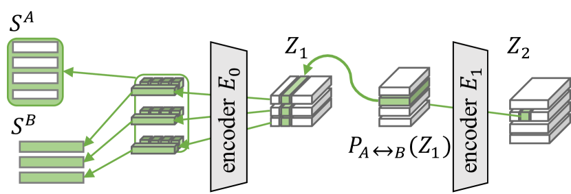
Figure 9: Backward path of DBM (single-stream architecture) from $ij$-th feature in $Z_{2}$, where the stream refers to all the elements in $S^{A}$ and $S^{B}$. This structure is common with SSWN.

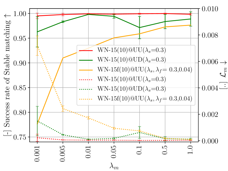
Figure 10: Sensitivity against $\lambda_{m}$

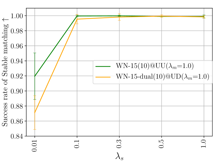
Figure 11: Sensitivity against $\lambda_{s}$

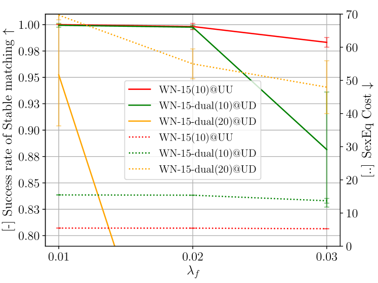
Figure 12: Sensitivity against $\lambda_{f}$

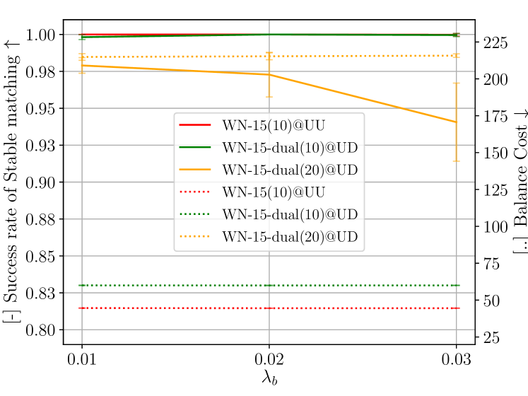
Figure 13: Sensitivity against $\lambda_{b}$

By stacking two or more FW layers, every latent feature of $ij$-th element in $Z^{*}_{\ell}$ ($\ell\geq 2$) has a receptive field that covers all over the preference lists. Fig. 8 illustrates the receptive field, where green elements are upstream components of the $ij$-th element, and $E_{0}$, $E_{1}$ are encoders that involve all the input into the calculation of each feature in the output sequence. Let us backtrack the path of back-propagation from the $ij$-th element in $Z^{A}_{2}$. It derives from the $i$-th row of $Z^{A}_{1}$ and the $i$-th column of $Z^{B}_{1}$. Focusing on the $i$-th column (e.g., the green column) of $Z^{B}_{1}$, each element (in the $k$-th row) derives from all the elements in the $k$-th row of $S^{B}$, plus all the elements in the $k$-th column of $S^{A}$. In this way, all the elements in $S^{A}$ and $S^{B}$ contribute to a column of $Z^{B}_{1}$, then an element of $Z^{A}_{2}$. Symmetrically, all the elements in $S^{A}$ and $S^{B}$ contribute to a column of $Z^{A}_{1}$, then an element of $Z^{B}_{2}$. Hence, we can see that stacking two FW layers can cover the entire bipartite graph in its reference.

We also visualize the back-propagation path of DBM in Fig. 9. DBM also covers the entire bipartite graph within two layers, but each encoder is used only for one direction (either weftwise or warpwise). Here, the path in Fig. 9 is identical with the lower path in Fig. 8. From this perspective, WeaveNet innately contains the path of DBM.

A.4 Loss Weights

Through the experiments, we set the loss weights $\lambda_{m}=1.0$, $\lambda_{s}=0.7$, and $\lambda_{f}=\lambda_{b}=0.01$ to train any learning-based methods. We adjusted these parameters in the following process.

As a preliminary model, we prepared WN-15 with a set encoder with $D=64$ and $D^{\prime}=256$. In this investigation, we used a balanced dataset UU and the most biased dataset UD.

Because we experimentally found the tendency that the model hardly outputs a stably matched solution without minimizing ${\mathcal{L}}_{m}$, we first tried to fix ${\mathcal{L}}_{m}$. Fig. 13 shows the success rate of stable matching with different ${\mathcal{L}}_{m}$ in the range $\{0.001,~{}0.005,~{}0.010,~{}0.050,~{}0.100,~{}0.500,~{}1.000\}$, where WN-15($n$) is the model trained and validated with the samples of $N=n$. From this result, we decided to set $\lambda_{m}=1.0$ and use it as the maximum weight among the loss weights.

Next, fixing $\lambda_{m}=1.0$, we observed the trend in success rate of stable matching against $\lambda_{s}$. Fig. 13 shows our investigation of ${\mathcal{L}}_{s}$ in the range $\{0.01,0.10,0.30,0.50,1.00\}$. Here, WN-dual is a WeaveNet variant to deal with the inconsistent distributions of UD (see B.2 for details of WN-dual). As a result, we found that $\lambda_{s}$ should simply be large enough (ca. $\lambda_{s}\geq 0.30$).

To investigate sensitivity of the model against $\lambda_{f}$ and $\lambda_{b}$, in this experiment, we set $\lambda_{s}=0.3$ as the minimum satisfiable value in Fig. 13, and obtained Figures 13 and 13. From these figures, we found that too-strong weights for fairness may disrupt stability, which matches a theoretical expectation. Hence, we decided to use $\lambda_{f}=\lambda_{b}=0.01$, which achieved the highest success rate of stable matching in the search range of $\{0.01,0.02,0.03\}$.

A.5 Network Architecture

We can customize the shape of WeaveNet architecture finely by using set encoders with different shapes in each FW layer; however, we avoided such a complex architecture design to simplify the analysis and decided to use common-shape set encoders for all $L$ FW layers. With this setting, we have only three hyper-parameters to decide the architecture: $L$, $D$, and $D^{\prime}$. The shortcut path is regularly connected to the input of $\ell$-th layer with an even number of $\ell$.

Name	$L$	$D$	$D^{\prime}$	# of params.	Stably Matched (%)
Deep	30	22	44	117k	95.7%
Wide1	15	32	64	119k	76.0%
Wide2	15	24	98	120k	73.1%

Table 5: Comparison in parameter efficiency among different shape architectures. Deep achieved the best success rate in stable matching despite its smallest architecture.

Table 5 shows the success rate of stable matching after 100,000 iterations of training. Here, we drew samples from the UU distribution with $N=30$ for both training and validation. The result shows that the deepest model performs the best despite its smallest number of parameters. Hence, we decided to use the set encoder that has $D\leq 32$ and $D^{\prime}=2D$.

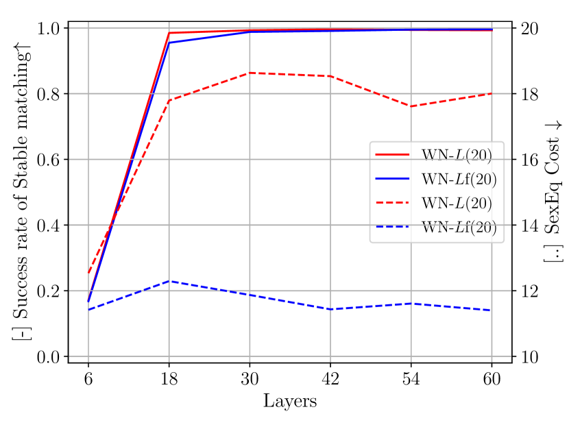
Figure 14: Success rate of stable matching (solid, $\uparrow$) and $SEq$ (dashed, $\downarrow$) according to $L$.

We further investigated the impact of network depth on the problem. To observe how the strongly NP-hard target increases the difficulty in optimization, we plotted both results by WN-$L$ and WN-$L$f with $L\in\{6,18,30,42,54,60\}$. Fig. 14 shows the trend of success rate against different $L$. Here, the models were trained and validated with the UU dataset at $N=20$. We can see from the result that $L=6$ is not enough to stably match samples of $N=20$, but $L=18$ is enough if only for that purpose. Besides, we observed that a deeper stack of layers tends to improve $SEq$ slightly.

Model	Encoder	$D$	$D^{\prime}$	Res.	# of params.
MLP-3	dense layer	100	-	w/o	28k
GIN-2	graph conv.	44	-	w/o	29k
DBM-6	max pooling	48	-	w/o	29k
DBM_A-6	self-attention	48	32	w/	28k
SSWN-6	set encoder	48	48	w/o	25k
SSWN-60	set encoder	64	64	w/	740k
WN-6	set encoder	24	48	w/o	25k
WN_A-6	self-attention	32	28	w/	29k
WN-18	set encoder	32	64	w/	143k
WN-60	set encoder	32	64	w/	493k
WN-80	set encoder	32	64	w/	659k

Table 6: Hyper-parameters for each baseline, where $D^{\prime}$ represents the length of key and query features for self-attention, and the max-pooling input for the set encoder. Note that the $D$-dimentional feature of WN is cross-concatenated and processed as a $2D$-dimensional features in the encoders.

A.6 Hyper-parameter Settings for the Other Baselines

Here, we denote the hyper-parameters for learning-based baseline methods, including those used in B.1 and B.2. The detail is summarized in Table 6. Note that MLP could not converge when more than three hidden layers are stacked. Hence, we set the number of layers to be three, as used in Li [2019]. For GIN Xu et al. [2019], we put two layers because the original paper reported it performs best. Besides that, some papers provide theoretical analyses that graph convolutional networks (GCNs) suffer from over-smoothing Li et al. [2018]; Oono and Suzuki [2020]. Namely, it loses the discriminative capacity for nodes on a dense graph when the layers are deeply stacked. This is exactly our case because a complete bipartite graph is always dense; its connection density is $N/(2N-1)(>1/2)$ (there are $2N^{2}$ edges among $2N(2N-1)$ possible edges). Hence, a deeper stack does not contribute to solving the problem.

Note that we used the same loss weights decided in A.4 for all the methods since the loss weights derive from the task property rather than the architecture. For simplicity in comparison, we also used the three hyper-parameters, $L$, $D$, and $D^{\prime}$, to identify the architecture following to A.5. We experimentally decided whether to use the residual structure or not for the models which have more than four layers. Hence, the shown results are always better ones.

Appendix B Additional Experiments

B.1 Additional Learning-based Baselines and Ablations.

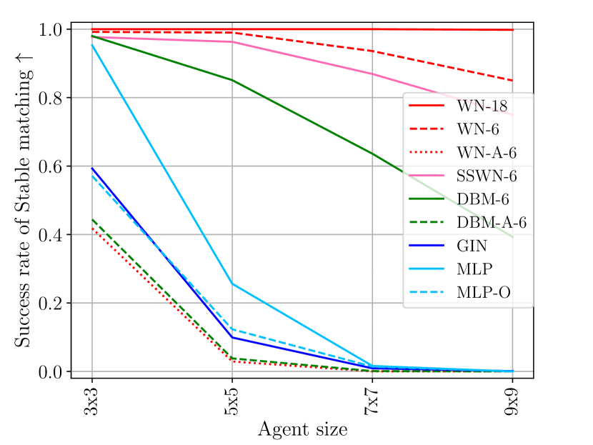
Figure 15: Change in success rate of stable matching ($\uparrow$) according to $N$, as a complement of Fig. 6.

We compared WeaveNet to more comprehensive baselines: a variation of MLP, DBM, WeaveNet, and a GCN model. Fig. 15 shows the results.

MLP-O is a variant of MLP that faithfully follows the loss functions proposed in Li [2019]. The difference is in the matrix constraint loss function ${\mathcal{L}}_{m}$. Ours defined in Eq. (6) is cosine-distance based, while the one proposed in the original paper is Euclidean-distance based, which is

$$\begin{split}{\mathcal{L}}_{m}(\hat{m}^{A},\hat{m}^{B})&=\sum_{\{i,j\}\in A\times B}|\hat{m}^{A}_{ij}-\hat{m}^{B}_{ji}|.\end{split}$$ (12)

The above loss function restricts $i$-th column and $i$-th row of $\hat{m}$ to be the same point in the $N\times M$ space. In other words, the column and row must match in a scale variant manner. We considered that this is unnecessarily strict for maintaining $\hat{m}$ to be symmetric. Hence we adopted the cosine distance for ${\mathcal{L}}_{m}$. In Fig. 15, we observed that MLP has a clear performance gain from MLP-O by our cosine-distance-based ${\mathcal{L}}_{m}$.

GIN is the state-of-the-art GCN architecture Xu et al. [2019]. Some readers may consider GCNs as the solution to this problem. We put two GIN layers followed by one Linear layer that outputs $\hat{m}$ as a flat vector as MLP. From the result, we confirmed that the GCN is not suitable to solve this problem.

DBM proposed in Gibbons et al. [2019] has two variations; one uses max-pooling with one convolutional layer as the layer-wise encoder (DBM) and self-attention (DBM_A). We also integrated self-attention into the WeaveNet architecture (WN_A-6) to complete the comparison of the encoder choice. As a result, we have confirmed that self-attention does not work well for stable matching problem.

Agents ($N\times M$)	20$\times$20					30$\times$30
Datasets (Distribution Type)	UU	DD	GG	UD	Lib	UU	DD	GG	UD	Lib
WN-60f-sym	11.44	6.32	15.34	81.21	14.39	16.07	9.64	26.46	194.24	21.16
Stably Matched (%)	99.10	99.40	99.40	96.00	99.50	98.10	99.00	98.00	81.50	98.80
WN-60f-asym	-	-	-	71.18	14.44	-	-	-	162.61	21.29
Stably Matched (%)	-	-	-	99.50	99.80	-	-	-	93.90	98.60
WN-60f-dual	-	-	-	71.25	14.58	-	-	-	163.71	22.12
Stably Matched (%)	-	-	-	98.50	99.60	-	-	-	94.80	97.50
WN-60f(20)	11.49	6.20	15.30	71.10	14.40	16.66	9.55	26.57	162.91	21.82
Stably Matched (%)	98.90	99.50	99.40	99.60	99.30	94.60	97.30	95.70	91.30	97.70
SSWN-60f	12.82	7.41	16.62	70.94	15.20	19.13	12.76	28.33	160.83	22.45
Stably Matched (%)	95.80	99.20	96.50	92.40	97.90	90.00	97.50	89.00	69.20	92.30
WN-60f+Hung	11.51	6.35	15.37	71.18	14.45	16.14	9.69	26.58	162.73	21.32
Stably Matched (%)	99.80	99.90	100.00	99.60	100.00	99.70	99.90	99.90	95.20	99.20

Table 7: Ablation study for the network architecture difference with $SEq$ ($\downarrow$) and the success rate of stable matching ($\uparrow$). The scores shown in Table 3 are underlined.

Agents ($N\times M$)	20$\times$20					30$\times$30
Datasets (Distribution Type)	UU	DD	GG	UD	Lib	UU	DD	GG	UD	Lib
WN-60b-sym	71.29	138.57	106.50	141.96	65.59	137.70	301.08	221.12	315.51	127.05
Stably Matched (%)	98.00	99.10	98.60	97.30	98.90	97.90	98.60	93.70	80.30	98.10
WN-60b-asym	-	-	-	140.72	65.63	-	-	-	313.11	127.12
Stably Matched (%)	-	-	-	99.80	99.10	-	-	-	98.80	98.00
WN-60b-dual	-	-	-	141.20	65.70	-	-	-	314.79	127.25
Stably Matched (%)	-	-	-	99.60	99.30	-	-	-	98.90	97.90
WN-60b(20)	71.05	138.53	106.13	140.81	65.53	137.06	301.21	220.23	313.68	127.62
Stably Matched (%)	98.50	98.80	99.50	99.70	98.80	96.10	96.70	95.00	88.90	93.80
SSWN-60b	76.54	139.29	107.58	141.37	66.99	150.88	302.90	223.62	314.91	129.52
Stably Matched (%)	92.60	98.50	98.40	99.60	98.60	79.80	96.70	93.90	94.0	92.80
WN-60b+Hung	71.45	138.60	106.55	140.73	65.68	137.92	301.14	221.42	313.13	127.22
Stably Matched (%)	99.90	99.90	99.60	99.90	100.00	99.00	99.90	96.90	99.30	99.20

Table 8: Ablation study for the network architecture difference with $Bal$ ($\downarrow$) and the success rate of stable matching ($\uparrow$). The scores shown in Table 3 are underlined.

B.2 Additional Ablation in $N=20,~{}30$

We provide a detailed ablation study to finely analyze the symmetric and asymmetric variants, the effect of two-stream architecture, the size of training samples, and the binarization operation.

First, we refer to the symmetric and asymmetric variants of WN-60f/b as WN-60f/b-sym and WN-60f/b-asym, respectively. Note that both models have the two-stream architecture, but sym shared batch normalization layers and asym does not. In addition, asym has an additional channel in inputs for side-identifiable code. In addition to them, we further prepared WN-60f/b-dual, a model that separately holds the entire set encoder for $Z^{A}_{\ell}$ and $Z^{B}_{\ell}$ at each layer to deal with asymmetric inputs. Since UD is a highly asymmetric dataset, the symmetric variant (WN-60f/b-sym) does not work appropriately while the asymmetric variants (asym and dual) could deal with it. In the dataset Lib, where we assumed an unknown bias strength, asym worked as well as sym and dual. This result showed that we can safely apply the asymmetric variation for any situation.

Comparing asym with dual, asym marked slightly smaller fairness costs than dual while keeping comparative success rate in stable matching. This result experimentally confirmed the parameter efficiency of asym against dual since dual has roughly twice more parameters than asym.

Second, to investigate the effect of choosing different training sample size, we prepared WN-60f/b(20), a model trained by samples of $N=20$, and applied it to test datasets of $N=20,~{}30$. The asymmetric variant was applied for UD and Lib. From the results, we confirmed that the models trained with $N=30$ has no degradation from WN-60f/b(20) even when tested at $N=20$. In contrast, WN-60f/b(20) did not perform well when applied to the samples of $N=30$. This trend implies that we should train the model with a larger $N$ to cover a wide range of input-size variations.

Third, SSWN-60, a single-stream WeaveNet with set encoders, was prepared to measure the contribution of the two-stream architecture. SSWN-60f/b achieved consistently worse result than WN-60f/b (underlined), and collapsed in UD ($N=30$) in Table 3 and UU ($N=30$) in Table 3. These results experimentally proved the importance of the two-stream structure.

Finally, to avoid an increase of theoretical calculation cost, WeaveNet applied ${\rm argmax}$ operation to binarize $\hat{m}$ rather than the Hungarian algorithm, whose calculation cost is $O(N^{3})$. To demonstrate how well the network maintains ${\rm argmax}(\hat{m})$ to be a matching, we compared the result with those obtained with the Hungarian algorithm (WN-60f+Hung). Again, the asymmetric variant was applied for UD and Lib. From the result, we confirmed that WN-60f/b+Hung achieved higher success rates in stable matching while worse $SEq$ and $Bal$ costs. This behavior implies that the output matched only by the Hungarian algorithm tends to have higher fairness costs.

To obtain further insight, we prepared Table 9, which summarizes the difference w/ and w/o the Hungarian algorithm at $N=100$. In this setting, we have more samples with which WN-80f/b fails to even obtain one-to-one matching by the ${\rm argmax}$ binarization. Binarization by the Hungarian algorithm forces such failure estimation $\hat{m}$ to be a matching; however we obtained only 5.0% additional stable matchings from the 13.4% failure cases with WN-80f, and 7.5% from 19.8% failure cases with WN-80b. A similar number of cases resulted in matchings with more than three blocking pairs.

From these results, we concluded that the Hungarian algorithm does not essentially improve the quality of fair stable matching, although it ensures $\hat{m}$ to be a one-to-one matching.

#Block. Pairs	WN-80f	+Hung.	WN-80b	+Hung.
0	84.4%	89.4%	73.2%	80.8%
1	2.2%	4.6%	6.7%	10.9%
2	0.0%	0.4%	0.3%	1.2%
$\geq 3$	0.0%	5.6%	0.0%	7.1%
Fail	13.4%	-	19.8%	-

Table 9: Number of blocking pairs in the estimated matching with UU $N=100$. Fail counts outputs that are not a one-to-one matching. Outputs with no blocking pairs are stable matchings.

Appendix C Data for Reproduction

C.1 Calculation Time and Computing Infrastructure

We trained and tested the learning-based models used in the experiments on a single GPU (Tesla V100, memory size 16GB) mounted on NVIDIA DGX-1. We developed the environment on Ubuntu18.04.

Elapsed Time	for training	for test
	200,000 iters.	1,000 samples
WN-6  ($N=10$)	10.39 hours	5.82 s
WN-18 ($N=10$)	13.10 hours	14.83 s
WN-60 ($N=20$)	30.10 hours	75.15 s
WN-60 ($N=30$)	43.58 hours	74.10 s
WN-80 ($N=100$)	111.10 hours	103.66 s

Table 10: Elapsed time for training and testing the models.

The above training required less than 16GB of memory space in our setting as long as the batch size is no larger than $8$. The training and inference time are summarized in Table 10.

C.2 Dataset

We implemented the data generator for UU, DD, GG, UD, and Lib following the explanation in Tziavelis et al. [2019] since they are not provided by the authors. In the process, we also extracted the distribution of the LibimSeTi dataset Brozovsky and Petricek [2007], where the original data of the LibimSeTi dataset is accessible in http://www.occamslab.com/petricek/data/. We filtered out data that do not have bidirectional preference rank, as stated in Tziavelis et al. [2019]. We yielded the validation and test datasets with a fixed random seed to make them reproducible.

All the code for data generation is included in the submission (with the random seeds and fairness costs of each sample obtained by the traditional algorithmic baselines). They will become publicly available at the timing of publication of this paper.

References

- Ahuja et al. [2007] Ravindra K Ahuja, Arvind Kumar, Krishna C Jha, and James B Orlin. Exact and heuristic algorithms for the weapon-target assignment problem. Operations research, 55(6):1136–1146, 2007.
- Brozovsky and Petricek [2007] Lukas Brozovsky and Vaclav Petricek. Recommender system for online dating service. In Proceedings of Conference Znalosti 2007, Ostrava, 2007.
- Chen et al. [2018] Jiehua Chen, Rolf Niedermeier, and Piotr Skowron. Stable marriage with multi-modal preferences. In Proceedings of ACM Conference on Economics and Computation, page 269â286, 2018.
- Dworczak [2016] Piotr Dworczak. Deferred acceptance with compensation chains. In Proceedings of the 2016 ACM Conference on Economics and Computation, pages 65–66, 2016.
- Emami et al. [2020] Patrick Emami, Panos M. Pardalos, Lily Elefteriadou, and Sanjay Ranka. Machine learning methods for data association in multi-object tracking. ACM Computing Surveys, 53(4), 2020.
- Fathony et al. [2018] Rizal Fathony, Sima Behpour, Xinhua Zhang, and Brian Ziebart. Efficient and consistent adversarial bipartite matching. In Proceedings of International Conference on Machine Learning, pages 1457–1466, 2018.
- Feder [1992] Tomás Feder. A new fixed point approach for stable networks and stable marriages. Journal of Computer and System Sciences, 45(2):233–284, 1992.
- Feder [1995] Tomás Feder. Stable networks and product graphs. American Mathematical Society, 1995.
- Gale and Shapley [1962] David Gale and Lloyd S Shapley. College admissions and the stability of marriage. The American Mathematical Monthly, 69(1):9–15, 1962.
- Gibbons et al. [2019] Daniel Gibbons, Cheng-Chew Lim, and Peng Shi. Deep learning for bipartite assignment problems. In Proceedings of IEEE International Conference on Systems, Man and Cybernetics, pages 2318–2325, 2019.
- Gupta et al. [2019] Sushmita Gupta, Sanjukta Roy, Saket Saurabh, and Meirav Zehavi. Balanced stable marriage: How close is close enough? In Workshop on Algorithms and Data Structures, pages 423–437, 2019.
- Gusfield and Irving [1989] Dan Gusfield and Robert W Irving. The stable marriage problem: structure and algorithms. MIT press, 1989.
- Gusfield [1987] Dan Gusfield. Three fast algorithms for four problems in stable marriage. SIAM Journal on Computing, 16(1):111–128, 1987.
- Irving et al. [1987] Robert W Irving, Paul Leather, and Dan Gusfield. An efficient algorithm for the “optimal” stable marriage. Journal of the ACM, 34(3):532–543, 1987.
- Iwama et al. [2010] Kazuo Iwama, Shuichi Miyazaki, and Hiroki Yanagisawa. Approximation algorithms for the sex-equal stable marriage problem. ACM Transaction on Algorithms, 7(1), 2010.
- Kato [1993] Akiko Kato. Complexity of the sex-equal stable marriage problem. Japan Journal of Industrial and Applied Mathematics, 10(1):1, 1993.
- Kingma and Ba [2015] Diederik P. Kingma and Jimmy Ba. Adam: A method for stochastic optimization. In Proceedings of International Conference on Learning Representations, 2015.
- Kuhn [1955] Harold W Kuhn. The hungarian method for the assignment problem. Naval research logistics quarterly, 2(1-2):83–97, 1955.
- Li et al. [2018] Qimai Li, Zhichao Han, and Xiao-Ming Wu. Deeper insights into graph convolutional networks for semi-supervised learning. In Proceedings of AAAI Conference on Artificial Intelligence, pages 3538–3545, 2018.
- Li [2019] Shira Li. Deep Learning for Two-Sided Matching Markets. Bachelor’s thesis, Harvard University, 2019.
- McDermid and Irving [2014] Eric McDermid and Robert W Irving. Sex-equal stable matchings: Complexity and exact algorithms. Algorithmica, 68(3):545–570, 2014.
- Oono and Suzuki [2020] Kenta Oono and Taiji Suzuki. Graph neural networks exponentially lose expressive power for node classification. In Proceedings of International Conference on Learning Representations, 2020.
- Qi et al. [2017] Charles R. Qi, Hao Su, Kaichun Mo, and Leonidas J. Guibas. PointNet: Deep learning on point sets for 3D classification and segmentation. In Proceedings of IEEE Conference on Computer Vision and Pattern Recognition, July 2017.
- Tziavelis et al. [2019] Nikolaos Tziavelis, Ioannis Giannakopoulos, Katerina Doka, Nectarios Koziris, and Panagiotis Karras. Equitable stable matchings in quadratic time. In Proceedings of Advances in Neural Information Processing Systems, pages 457–467, 2019.
- Wang et al. [2019] Yansheng Wang, Yongxin Tong, Cheng Long, Pan Xu, Ke Xu, and Weifeng Lv. Adaptive dynamic bipartite graph matching: A reinforcement learning approach. In Proceedings of IEEE International Conference on Data Engineering, pages 1478–1489, 2019.
- Xu et al. [2019] Keyulu Xu, Weihua Hu, Jure Leskovec, and Stefanie Jegelka. How powerful are graph neural networks? In Proceedings of International Conference on Learning Representations, 2019.
- Zaheer et al. [2017] Manzil Zaheer, Satwik Kottur, Siamak Ravanbakhsh, Barnabas Poczos, Russ R Salakhutdinov, and Alexander J Smola. Deep sets. In Proceedings of Advances in Neural Information Processing Systems, volume 30, pages 3391–3401, 2017.