Online Estimation with Rolling Validation:
Adaptive Nonparametric Estimation with Stream Data

Abstract

Online nonparametric estimators are gaining popularity due to their efficient computation and competitive generalization abilities. An important example includes variants of stochastic gradient descent. These algorithms often take one sample point at a time and instantly update the parameter estimate of interest. In this work we consider model selection and hyperparameter tuning for such online algorithms. We propose a weighted rolling-validation procedure, an online variant of leave-one-out cross-validation, that costs minimal extra computation for many typical stochastic gradient descent estimators. Similar to batch cross-validation, it can boost base estimators to achieve a better, adaptive convergence rate. Our theoretical analysis is straightforward, relying mainly on some general statistical stability assumptions. The simulation study underscores the significance of diverging weights in rolling validation in practice and demonstrates its sensitivity even when there is only a slim difference between candidate estimators.

1 Introduction

Online estimators are a collection of statistical learning methods where the estimate of the parameter of interest is sequentially updated during the reception of a stream of data ([14], Section 3). In contrast to traditional batch (or offline) estimators that learn from the entire training data set all at once, online estimators gradually improve themselves after more data points are processed. They have gained popularity in recent years especially due to their lower computational expense compared to traditional batch learning methods. This characteristic has made online learning particularly attractive in scenarios where data arrives continuously and computational resources are limited. Even with a complete, “offline” data set in hand, online methods are still routinely applied given their fast training speed and competitive prediction quality. Over the past two decades, there has been significant progress in the development of online estimators, both in terms of their implementation and our understanding of their statistical properties [7, 8, 19, 25, 32, 17]. Several works [3, 8, 35] have shown that estimators trained with stochastic gradient descent (SGD) can achieve certain statistical optimality.

The performance of nonparametric estimators, usually measured as the predictive accuracy, often crucially depends on some hyperparameters that need to be specified in the algorithm, such as the number of basis functions in basis expansion-based algorithm and step size in gradient-based algorithms. Selecting a good hyperparameter value is both practically important and theoretically desirable. Cross-validation (CV) is one of the most widely used techniques in batch learning to assess the generalization ability of a fitted model and perform model selection. The data is divided into multiple (say, $K$) equal-sized folds. The model is then trained on $K-1$ folds and evaluated on the remaining fold. This process rotates over the holdout fold and takes the average holdout validation accuracy as the overall assessment. Although CV has a long history [24, 20] and arguably the most implemented model selection methods in practice [6, 21, 1, 22, 9], its practical performance and theoretical investigation leaves many questions to be answered. There is strong empirical evidence that cross-validation tends to give slightly biased model selection results, and several empirical adjustments have been proposed, such as the “0.632 rule” [10] and the “one standard error rule” [27]. Theoretically, while CV is known to be risk-consistent [5, 15] under very general conditions when it comes to model selection, it is shown [31, 12] that batch CV may not consistently select the correct model under some natural scenarios.

In this work, we study the problem of online model/hyperparameter selection using a variant of cross-validation. To begin with, we must clarify what it means by model selection consistency in online estimation, which turns out quite different between the batch setting and the online setting. In the theory of nonparametric and/or high-dimensional statistics, the optimal hyperparameter is determined by three components: the complexity of parameter space, the amount of noise in the data, and the sample size. Therefore, in a batch setting, where the sample size is known and fixed, one can simply compare different hyperparameters. However, in the online setting, the sample size keeps increasing and the optimal hyperparameter must change accordingly as predicted by the theory. For example, the optimal lasso penalty should scale inversely as the square root of the sample size. In this work, we propose to focus on selecting among sequences of hyperparameters rather than among individual hyperparameters. More specifically, we are given a collection of sequences of hyperparameters, each specified by a particular function form with respect to the sample size, and the inference task is to find out the optimal sequence that gives the best prediction accuracy. When the $n$-th sample is revealed to the estimation algorithm, it updates the current estimate, for example, by taking an SGD step. The specifics of this update, such as the step size and/or the model capacity of the update, are determined by the $n$-th element of the hyperparameter sequence, $\lambda_{n}$. When the next sample arrives, the update procedure will iterate with $\lambda_{n+1}$. More detailed discussion and motivation of the tuning sequence selection problem and its difference from the batch tuning problem is given in Section 2.2.

To select the best hyperparameter sequence, we propose a new methodology called “weighted rolling validation”, which can be viewed as a variant of leave-one-out cross-validation adapted to online learning. Unlike batch learning, where data is artificially split into fitting and validation folds, in the online setting the “next data point” naturally becomes the validating sample for the current estimate. Such a validation scheme, called “rolling validation” (RV), efficiently exploits the computational advantage of online learning algorithms, because the standard leave-one-out batch CV requires re-fitting the model $n$ times, whereas rolling validation incurs no extra fitting at all. Our theoretical and methodological framework for rolling validation allows for different weights to different time points in calculating the cumulative validated risks. Such weights add additional flexibility to the algorithm design and show remarkable practical improvements. Our main theoretical result states that, under certain stability conditions on the fitting algorithms, the weighted rolling validation can select the best hyperparameter sequence with probability tending to one as the sample size diverges to infinity, provided the candidate sequences are sufficiently different. This result agrees with the existing results for batch CV. If the candidate sequences are too similar, such as both being $\sqrt{n}$-consistent, then CV-based model selection is known to be inconsistent [23, 33, 31].

Related work.

Procedures that are formally similar to RV have been implemented in real-world data analysis, especially for time series data [2, 30], but neither have they been implemented nor formally well-studied in the context of online adaptive nonparametric estimation. In the field of time series analysis, these procedures are referred to as “expanding window cross-validation” or “walk-forward validation”. To the best of the authors’ knowledge, the earliest related work was published in 1972 ([2], page 216), which implements a similar performance metric for long-range market forecasting tasks. The idea of RV is also mentioned in an earlier review paper [26], under the name “rolling-origin calibration”. In a more recent study [4], the authors applied unweighted RV—referred to as “online cross-validation” in their work—to ensemble learning and present some favorable guarantees of the proposed estimators. Compared with their work, we explicitly engage with nonparametric procedures, elucidate what the hyperparameters are in these settings, and go into more details of the theoretical analysis. Moreover, our proposed weighted RV statistics can much better trace the transition of estimators’ generalization error than the unweighted version, which may take $10$k more samples for the latter to make the correct choice in some typical settings (Section 6).

Notation.

We will use $\mathbb{R}$ to denote real numbers and $\mathbb{N}^{+}$ to denote the set of positive integers. For any vector $x$ in $\mathbb{R}^{p}$ or $(\mathbb{N}^{+})^{p}$, we use $x[j]$ to denote its $j$-th element. Notation $a\vee b=\max\{a,b\}$ for $a,b\in\mathbb{R}$. For a random variable $X$ and a probability distribution $P$, the notation $X\sim P$ means “the distribution of $X$ is $P$”. In some conditional expectation notation such as $E[f(X,Y)|F^{i}]$, we use $F^{i}$ to denote the $\sigma$-algebra generated by sample $\{(X_{j},Y_{j}),1\leq j\leq i\}$. We use $\delta_{jk}$ to represent Kronecker delta: $\delta_{jk}=1$ when $j=k$ and $\delta_{jk}=0$ otherwise. The inequality $a\lesssim b,a,b\in\mathbb{R}$ means $a\leq Cb$ for some constant $C$, but the value of $C$ may be different from line to line.

2 Stochastic Approximation and the Problem of Online Model Selection

In a typical statistical learning scenario, we have sample points of a pair of random variables $(X,Y)\in\mathbb{R}^{p}\times\mathbb{R}^{1}$ with joint distribution $P$, and want to minimize the predictive risk over a class $\mathcal{F}$ of regression functions: $\min_{f\in\mathcal{F}}E_{(X,Y)\sim P}[l(f;X,Y)]$ under a loss function $l(\cdot)$. We denote the marginal distribution of $X$ as $P_{X}$ and assume that $E(Y^{2})<\infty$. For regression problems, we typically consider the squared loss $l(f;X,Y)=(f(X)-Y)^{2}$. When $\mathcal{F}$ is the function space of mean-square integrable functions $L_{2}(P(X))$, the corresponding minimizer

$$f_{0}=\operatorname*{argmin}_{f\in L_{2}(P(X))}E[(f(X)-Y)^{2}]$$ (1)

is the conditional mean function or the true regression function.

In contrast to batch learning where all the data is available at once, stream samples are usually revealed to the researchers continuously. For the sake of storage and computing, it is more common to treat large data sets as a data stream and apply online methods. The estimates need to be frequently updated whenever new samples arrive. For simplicity, we set the initial estimate to the zero function without loss of generality. When a new sample $(X_{i+1},Y_{i+1})\sim P(X,Y)$ arrives, the algorithm uses this new piece of information to update the current estimate, denoted as $\hat{f}_{i}$, to a new estimate $\hat{f}_{i+1}$. One may convert any batch estimator to an online one by storing all the past data and refitting the whole model repeatedly. But this is often computationally infeasible. For example, fitting a kernel ridge regression estimator using $i$ samples (by matrix inversion) requires $i^{3}$-order computation. This would result in a cumulative $n^{4}$ computation to process $n$ samples in an online fashion. Moreover, batch estimators often need to load the whole data set into the memory, causing significant storage costs, whereas genuine online algorithms only need to load a small portion of data and have a much lower memory footprint.

For genuine online estimators, the new estimate $\hat{f}_{i+1}$ can be written as the output of a pre-defined $\text{Update}(\cdot)$ mapping, whose inputs are the current estimate $\hat{f}_{i}$, the new sample $(X_{i+1},Y_{i+1})$ and hyperparameters $\lambda_{i}\in\mathbb{R}^{\Lambda}$, for some $\Lambda\in\mathbb{N}^{+}$. Formally,

$$\hat{f}_{0} \leftarrow 0$$ (2)

$$\hat{f}_{i+1} \leftarrow\operatorname{Update}\left(\hat{f}_{i},\left(X_{i+1},Y_{i+1}\right),\lambda_{i}\right).$$

In such an online scheme, it is important that the updating function depends on the past data only through the current estimate $\hat{f}_{i}$ for computational efficiency. Although Update$(\cdot)$ is a fixed function of its components, the varying hyperparameter $\lambda_{i}$ allows much flexibility in the overall algorithm.

2.1 Examples of Online Estimators and their Hyperparameters

In this section, we review the basic ideas of stochastic approximation and SGD, and the explicit forms of hyperparameter sequences. Assume the conditional mean function $f_{0}$ is linear: $f_{0}\in\mathcal{F}_{linear}$, so that for each $f\in\mathcal{F}_{linear}$, there exists a vector $\beta\in\mathbb{R}^{p}$ such that $f(X;\beta)=X^{\top}\beta$. Then we arrive at a parametric stochastic optimization problem:

$$\min_{\beta\in\mathbb{R}^{p}}E\left[l(f(\cdot;\beta);X,Y)\right]$$ (3)

The gradient descent method, a basic numerical optimization technique, uses the following iterative estimation procedure: First, initialize $\tilde{\beta}_{0}=0$, then iteratively update the estimate using the gradient descent formula:

$$\tilde{\beta}_{i+1}\leftarrow\tilde{\beta}_{i}-\gamma_{i}\nabla_{\beta}E\left[l(f(\cdot;\beta);X,Y)\right]\big{|}_{\tilde{\beta}_{i}},$$ (4)

where $\gamma_{i}\in\mathbb{R}^{+}$ is a pre-specified sequence of step sizes (or learning rates). In practice the expectation $E[\cdot]$ cannot be evaluated and must be approximated from the data. Typical stochastic gradient descent procedures replace it with a one-sample (or mini-batch) estimate. In the case of linear regression:

$$\tilde{\beta}_{i+1}\leftarrow\tilde{\beta}_{i}-\gamma_{i}\left.\nabla_{\beta}\left(X_{i+1}^{\top}\beta-Y_{i}\right)^{2}\right|_{\tilde{\beta}_{i}}=\tilde{\beta}_{i}+2\gamma_{i}\left(Y_{i+1}-X_{i+1}^{\top}\tilde{\beta}_{i}\right)X_{i+1}.$$ (5)

Since $\tilde{f}_{i}(X)=X^{\top}\tilde{\beta}_{i}$ is uniquely determined by the coefficients, we have our first concrete example of the stochastic approximation rule (2). Here the hyperparameter sequence is a sequence of real numbers $\lambda_{i}=\gamma_{i}\in\mathbb{R}^{1}$. Alternatively, we can also re-write the above iteration in a function-updating style:

$$\tilde{f}_{i+1}(\cdot)\leftarrow\tilde{f}_{i}(\cdot)+2\gamma_{i}\left(Y_{i+1}-\tilde{f}_{i}\left(X_{i+1}\right)\right)\sum_{k=1}^{p}\phi_{k}\left(X_{i+1}\right)\phi_{k}(\cdot).$$ (6)

The function $\phi_{k}:\mathbb{R}^{p}\rightarrow\mathbb{R}$ maps a $p$-dimensional vector to its $k$-th entry $\phi_{k}(X)=X[k]$. We write in this more intricate format to make the above updating rule more comparable with the rest of this section. The Polyak-averaging of $\{\tilde{f}_{i}\}$:

$$\hat{f}_{i}=i^{-1}\sum_{m=1}^{i}\tilde{f}_{m}=\frac{i-1}{i}\hat{f}_{i-1}+\frac{1}{i}\tilde{f}_{i}$$ (7)

is shown [3] to achieve the parametric minimax rate of estimating $f_{0}$ when the model is well-specified.

Now we turn to nonparametric online estimation with a diverging model capacity. In this case, the tuning hyperparameter at each step usually involves a truncation dimension. We illustrate this issue using the reproducing kernel stochastic gradient descent estimator (kernel-SGD). Let $\mathcal{K}(\cdot,\cdot):\mathbb{R}^{p}\times\mathbb{R}^{p}\rightarrow\mathbb{R}$ be a reproducing kernel, with eigen-value/eigen-function pairs $(q_{k},\phi_{k}(\cdot):k\geq 1)$. The kernel-SGD update rule is

$$\tilde{f}_{i+1}(\cdot) \leftarrow\tilde{f}_{i}(\cdot)+\gamma_{i}\left(Y_{i+1}-\tilde{f}_{i}\left(X_{i+1}\right)\right)\mathcal{K}\left(X_{i+1},\cdot\right)$$ (8)

$$=\tilde{f}_{i}(\cdot)+\gamma_{i}\left(Y_{i+1}-\tilde{f}_{i}\left(X_{i+1}\right)\right)\sum_{k=1}^{\infty}q_{k}\phi_{k}\left(X_{i+1}\right)\phi_{k}(\cdot).$$

This is our second example of the abstract updating rule (2). The related rate-optimal estimator [8] is its Polyak-averaging $\hat{f}_{i}=i^{-1}\sum_{m=1}^{i}\tilde{f}_{m}$, which can also be updated as described earlier (7).

The performance of kernel SGD depends on the chosen kernel function $\mathcal{K}$ and the learning rate sequence $\gamma_{i}$. It is shown that a sequence of slowly decreasing step sizes $\gamma_{i}=Ai^{-\zeta}$ would lead to rate-optimal estimators, where $A$ is a positive constant and $\zeta$ is typically small, $\zeta\in(0,1/2)$. However, the best choice of $\zeta$ depends on the expansion coefficients $\langle f_{0},\phi_{k}\rangle_{L_{2}(P(X))}$ and its relative magnitude to the eigenvalues $q_{k}$, which is in general not available to the algorithm. Data-adaptive procedures of choosing $\gamma_{i}$ is needed for better performance of the kernel-SGD in practice. Since theoretical results told us a polynomially decreasing step size is enough, the task of selecting $\gamma_{i}$ can be reduced to selecting proper $A$ and $\zeta$. Our framework also allows a varying reproducing kernel such as Gaussian kernels with a varying bandwidth. In the language of (2), the hyperparameters $\lambda_{i}=\gamma_{i}$ is of one dimension when assuming the kernel function is pre-specified and is of two dimension $\lambda_{i}=(\gamma_{i},\sigma_{i})^{\top}$ when there is a varying kernel bandwidth $\sigma_{i}$.

The second line of the kernel-SGD update (8) also suggests a direct way to construct the update from basis expansions without specifying a kernel. Recently, [35] consider “sieve-type” nonparametric online estimators that explicitly use an increasing number of orthonormal basis functions $\{\phi_{k}:k\geq 1\}$, with updating rule

$$\tilde{f}_{i+1}(\cdot)\leftarrow\tilde{f}_{i}(\cdot)+\gamma_{i}\left(Y_{i+1}-\tilde{f}_{i}\left(X_{i+1}\right)\right)\sum_{k=1}^{J_{i}}k^{-2\omega}\phi_{k}\left(X_{i+1}\right)\phi_{k}(\cdot),$$ (9)

and the averaged version $\hat{f}_{i}$ is similarly updated as in (7). Here $\gamma_{i}$ is a learning rate sequence as before, $J_{i}$ is a positive integer indicating the number of basis functions used in the $(i+1)$-th update, and $\omega$ is a shrinkage parameter which in practice can be taken as $1/2$. Sieve-SGD is more flexible as it does not require knowing the kernel, and is computationally more efficient since $J_{i}$ is usually much smaller than $n$ for moderate-dimension problems (where we do not model $p$ increasing with $n$). Under the assumption that $f_{0}$ belong to some Sobolev ellipsoid $W(s)$ spanned by $\{\phi_{k}\}$:

$$W(s)=W(s;Q)=\left\{f=\sum_{k=1}^{\infty}\beta_{k}\phi_{k},\beta_{k}\in\mathbb{R}\mid\sum_{k=1}^{\infty}\left(\beta_{k}k^{s}\right)^{2}\leq Q^{2}\right\}\,,$$ (10)

[36] showed that the sieve-SGD has minimal space expense (computer memory cost) among all statistically near-optimal estimators. The rate optimal hyperparameters are

$$\gamma_{i}=Ai^{-(2s+1)^{-1}}\text{ and }J_{i}=Bi^{(2s+1)^{-1}}.$$ (11)

The hyperparameter sequence $\{\lambda_{i}\}$ of sieve-SGD (9) is typically of two-dimension: $\lambda_{i}=(\gamma_{i},J_{i})^{\top}$.

2.2 The Goals and Targets of Model Selection in Batch and Online Estimation

The goals of model selection are subtly different in batch and online estimation. In batch learning, the hyperparameter governs the static capacity (or flexibility) of an estimator for a fixed sample size and is meant to be optimized with respect to this fixed sample size. Suppose we have a batch data set of size $i$ and $K$ candidate estimates $\hat{f}^{(k)}_{i}(\cdot;\lambda^{(k)}),k=1,2,...,K$, each is trained with a candidate hyperparameter vector $\lambda^{(k)}$, the goal of batch model selection at sample size $i$ is finding $k_{i}^{*}$ such that

$$k_{i}^{*} =\operatorname*{argmin}_{k\in\{1,..,K\}}r(\hat{f}^{(k)}_{i}),$$ (12)

$$\text{ where }r(\hat{f}^{(k)}_{i}) :=E\left[\left\|\hat{f}_{i}^{(k)}-f_{0}\right\|_{L_{2}\left(P_{X}\right)}^{2}\right].$$

The sample size $i$ is fixed in this batch setting. However, for online learning, the hyperparameter sequence governs how fast the model capacity increases as more training sample size increases and the model selection concerns how fast the risks decrease. Suppose we have a data stream and $K$ candidate estimate sequences $\{\hat{f}^{(k)}_{i}(\cdot;\lambda^{(k)}_{i}),i=1,2,...\},k=1,2,...,K$, each is trained with a hyperparameter sequence $\{\lambda^{(k)}_{i},i=1,...\}$. The goal of online model selection, in this paper, is to find the $k^{*}$ that eventually dominates all other candidates as the sample size increases:

$$\limsup_{i\rightarrow\infty}\ r(\hat{f}^{(k^{*})}_{i})/r(\hat{f}^{(k)}_{i})<1,\text{ for all }k\in\{1,...,K\}\backslash\{k^{*}\},$$ (13)

provided such a $k^{*}$ exisits.

We take sieve-type estimators as an example. For brevity of discussion, we omit the step-size $\gamma_{i}$ and focus only on the number of bases $J_{i}$, while keeping in mind that the full candidate grid should be formed in the 3-dimension space for $(A,B,s)$. Consider estimators of the form $\hat{f}_{i}(\cdot;J_{i})=\sum_{k=1}^{J_{i}}\beta_{k}\phi_{k}(\cdot)$, where the estimate can be written as a weighted combination of some pre-specified basis functions $\{\phi_{k}\}$. In the batch setting, we would estimate the weights $\{\beta_{k}\}$ using data $\{(X_{1},Y_{1}),...,(X_{i},Y_{i})\}$ once a candidate $J_{i}$ is proposed. So the overall batch estimation procedure can be described as follows: 1) collect $i$ samples and specify some grids $\{J^{(1)},..,J^{(K)}\}$; 2) apply cross-validation to fit $\hat{f}_{i}(\cdot;J^{(k)})$ and estimate its testing error $E[(Y-\hat{f}_{i}(X;J^{(k)}))^{2}]$. 3) Choose the $J^{*}\in\{J^{(1)},...,J^{(K)}\}$ that gives the lowest CV error and let $\hat{f}_{i}(\cdot;J^{*})=\sum_{k=1}^{J^{*}}\hat{\beta}_{k}\phi_{k}(\cdot)$ be our adaptive estimate. Such a selected tuning parameter $J^{*}$ is probably a good choice for that fixed sample size $i$, but probably not so when the sample size changes from $i$ to a larger value.

In contrast, online Sieve-SGD (9) is expected to use an increasing number of basis functions as training samples accumulate. Therefore an online model selection procedure should not aim at tuning the hyperparameter $J_{i}$ for a single sample size $i$. As we mentioned earlier, it is more natural to compare hyperparameter sequences. Our proposal is to integrate the theoretical “optimal converging/diverging order” (11) of the hyperparameters into the model selection procedure, and better connect the application and theoretical investigation. For instance, in the sieve-SGD setting, we consider some candidate grid $\{(B^{(1)},s^{(1)}),...,(B^{(K)},s^{(K)})\}$ over $(B,s)\in\mathbb{R}^{2}$ and (implicitly) construct $K$ infinite sequences of basis function numbers

$$\mathbf{J}^{(k)}=\left\{J_{i}^{(k)}=B^{(k)}i^{\left(2s^{(k)}+1\right)^{-1}},i=0,1,\ldots\right\}\,,~{}~{}k=1,2,\ldots,K.$$ (14)

We would, correspondingly, obtain $K$ sequences of estimators $\{\hat{f}^{(k)}_{i},i=1,2,...\},k=1,..,K$, each of them is trained with a different sequence of $\{J_{i}^{(k)}\}$. An online model selection procedure should point us to a choice of $\mathbf{J}_{i}^{(k)}$ that will eventually become the best for each $i$, which will further imply which $B$ and $s$ combination is the best based on available data.

3 Methods: Weighted Rolling Validation

In a stochastic approximation-type estimator (2), each new sample point is used to update the current estimates. Our method for tuning sequence selection is based on the idea of “rolling validation”, which, in addition to the estimate update, also uses the new sample point to update the online prediction accuracy of each candidate tuning sequence. Consider $K$ sequences of online estimators for $f_{0}$: $\{\hat{f}^{(k)}_{i}\},k=1,...,K$ with iterative formulas

$$\hat{f}_{i+1}^{(k)}=\operatorname{Update}\left(\hat{f}_{i}^{(k)},\left(X_{i+1},Y_{i+1}\right),\lambda_{i}^{(k)}\right).$$ (15)

To compare their online prediction accuracy, we consider the weighted Rolling Validation (wRV) statistic sequence for each candidate sequence:

$$RV_{i}^{(k)}=RV\left(\left\{\hat{f}_{l}^{(k)},l=1,\ldots,i\right\},\xi\right)=\sum_{l=1}^{i}l^{\xi}\left(\hat{f}_{l}^{(k)}\left(X_{l+1}\right)-Y_{l+1}\right)^{2},$$ (16)

where $\xi\geq 0$ is a rolling weight exponent to be chosen by the user. A positive $\xi$ will put more weight for larger values of $i$, which reflects the objective in (13) because we care more about the accuracy for larger values of $i$. For a finite sample size $i$, we use $\hat{k}^{*}_{i}=\arg\min_{1\leq k\leq K}RV_{i}^{(k)}$ to estimate $k^{*}$ as specified by (13).

Again, we emphasize that the quality of our estimate $\hat{k}^{*}_{i}$ should not be evaluated for any fixed finite sample, but rather in an asymptotic setting when $n\rightarrow\infty$, to match the sequential tuning objective (13). Therefore, we would hope that $\lim_{i\rightarrow\infty}P(\hat{k}^{*}_{i}=k^{*})=1$ under some reasonable conditions. Here we provide some quick intuitions. It is direct to see that $RV_{i}^{(k)}$ is an unbiased estimator of accumulated prediction error:

$$E\left[RV_{i}^{(k)}\right]=\sum_{l=1}^{i}l^{\xi}E\left[\left(\hat{f}_{l}^{(k)}(X)-Y\right)^{2}\right].$$ (17)

For the estimator to select the correct value of $k^{*}$, we need the following two conditions:

1. There is a gap between $E\left[RV_{i}^{(k^{*})}\right]$ and $\sup_{k\neq k^{*}}E\left[RV_{i}^{(k)}\right]$. This can be guaranteed by a more sophisticated form of (13).

2. The sample versions $RV_{i}^{(k)}$ do not deviate too far away from their expected values. This is technically more challenging as the dependence structure between the terms involved in $RV_{i}^{(k)}$ is complicated. We will resort to a stability-based argument.

A formal analysis will be presented in detail in Section 4, where the quality gap condition is given in 2 and the stability condition is given in 3.

In the literature, the unweighted version $\xi=0$ has been discussed [17], which corresponds to minimizing the unweighted rolling prediction risk ${\tt cum}_{i}^{(k)}=\sum_{l=1}^{i}E[(\hat{f}_{l}^{(k)}(X)-Y)^{2}]$. In another extreme case, when $\xi\rightarrow\infty$, the criterion corresponds to minimizing the local error ${\tt local}_{i}^{(k)}=E[(\hat{f}_{i}^{(k)}(X)-Y)^{2}]$ at time $i$. While the criterion based on ${\tt cum}_{i}$ can work in theory, its practical performance can be improved by using a positive finite $\xi$ that assigns more weights to more recent, larger values of $i$. On the other hand, the local criterion ${\tt local}_{i}^{(k)}$ may suffer from high variability due to the observation error carried in $Y$. We demonstrate such a phenomenon in our simulation (for a specific example, see Figure 2, A, model 8).

3.1 Computational Advantages of Rolling Validation

Input: A stream of training samples $(X_{i},Y_{i}),i\geq 1$. The estimator updating rule $\text{Update}(f,(X,Y),\lambda)$. Candidate hyperparameter sequences $\{\lambda^{(k)}_{i}:i\geq 1\}$, $1\leq k\leq K$, weight exponent $\xi$.

Initialize Estimators $\hat{f}^{(1)}=...=\hat{f}^{(K)}=0$. Rolling validation statistics $RV^{(1)}=...=RV^{(K)}=0$. Training sample index $i=0$.

while there are training samples not processed do

       Read in a new training sample $(X_{i+1},Y_{i+1})$
for $k$ in $1$ to $K$ do

             Calculate prediction from the $k$th estimate $\hat{Y}_{i+1}\leftarrow\hat{f}^{(k)}(X_{i+1})$
Update its RV statistics $RV^{(k)}\leftarrow RV^{(k)}+i^{\xi}(Y_{i+1}-\hat{Y}_{i+1})^{2}$
Update the estimator $\hat{f}^{(k)}\leftarrow\text{Update}(\hat{f}^{(k)},(X_{i+1},Y_{i+1}),\lambda^{(k)}_{i+1})$

       end for

      Output current selection $\hat{k}_{i}^{*}=\arg\min_{k}RV^{(k)}$
Increase training sample index $i\leftarrow i+1$

end while

Algorithm 1 Stochastic approximation with wRV for regression problems.

The RV statistics (16) is not only a natural target to examine when comparing online estimators, it can also save much computational expense when implemented efficiently. In Algorithm 1, we summarize our recommended framework of integrating model training and model selection in an online fashion. In contrast to the batch-learning scenario where training, validation and testing are typically done in three phases, our proposed procedure: 1) updates multiple estimators simultaneously; 2) calculates the RV statistics interchangeably with model training; and 3) offers a selected model at any time during the training process.

We take the kernel-SGD estimator (8) as an example to explicitly quantify the computational gain. Examining the updating rule, we can verify that both the trajectory functions $\{\tilde{f}_{i}\}$ and the (Polyak-averaged) estimator $\{\hat{f}_{i}\}$ are a linear combination of $i$ kernel functions “centered” at the past sample covariate vectors. Formally, there are some $\tilde{\beta}_{mi},\hat{\beta}_{mi}\in\mathbb{R}:$

$$\tilde{f}_{i}(\cdot)=\sum_{m=1}^{i}\tilde{\beta}_{mi}\mathcal{K}(X_{m},\cdot),\quad\hat{f}_{i}(\cdot)=\sum_{m=1}^{i}\hat{\beta}_{mi}\mathcal{K}(X_{m},\cdot).$$

Suppose evaluating one kernel function $\mathcal{K}(x,z)$ takes $O(p)$ computation—recall that $p$ is the dimension of $X_{i}$—then the majority of computation for the Update operator is calculating $\mathcal{K}(X_{i+1},X_{m})$ for all $m\in\{1,2,...,i\}$. This means $O((p+C)i)$ calculation when processing one sample $(X_{i+1},Y_{i+1})$, where $C$ is a small constant corresponding to the extra computation after evaluating all $\mathcal{K}(X_{i+1},X_{m})$. Moreover, the above computational expense accumulates to the order of $O((p+C)n^{2})$ for processing the first $n$ samples $\{(X_{1},Y_{1}),...,(X_{n},Y_{n})\}$. Naively training $K$ kernel-SGD estimators one at a time with $n$ samples would require $O(K(p+C)n^{2})$ computation if no intermediate quantities are saved. However, when the $K$ sequences of trajectories only differ at the learning rate $\gamma_{i}=Ai^{-\zeta}$, they can be simultaneously updated with only $O((p+KC)n^{2})$ computation, simply because the evaluated $\mathcal{K}(X_{i+1},X_{m})$ kernel value at each step can be shared between the estimators.

In addition to the computational gain for simultaneous training, these evaluated kernel values can be further shared with the the RV statistic calculation that only increases the total expense to at most $O((p+2KC)n^{2})$. This basically means that performance assessment is a “free-lunch” compared with the expense of training, without the need for a hold-out data for model selection. The only extra space expense is saving extra $K$ numbers $\{RV^{(k)}\}$. A similar calculation also holds for Sieve-SGD (9): the computational expense of training and validating $K$ estimators can be bounded by $O((p+2KC)nJ(n))$, where $J(\cdot)$ is largest basis number among the candidate $K$ estimators. For a fixed $p$, $J(n)$ is typically a diverging sequence such that $J(n)=o(\sqrt{n})$.

4 Consistency of Rolling Validation

In this section, we will investigate the statistical properties of the proposed rolling validation procedure for (non)parametric regression problems. In particular, we focus on whether wRV is able to select $k^{*}$ specified in (13) from a finite and fixed candidate set. Because the candidate set is finite and fixed, we can simply consider the case $K=2$, with two sequences of online estimators $\{h_{i}\}$ and $\{g_{i}\}$ of the conditional mean function $f_{0}$, we will show that when the online generalization errors of them are sufficiently different and stable under small perturbations of the training data, wRV can pick the better model with probability approaching one. This consistency result easily extends to any finite $K\geq 2$ by considering $k^{*}$ against each candidate and use union bound. Below we list the technical conditions.

First, we assume IID samples generated from a fixed underlying distribution.

Assumption 1 (A1, IID samples and finite noise variance).

The data points $\{(X_{i},Y_{i})\in\mathbb{R}^{p+1},i\geq 1\}$ are IID samples from a common distribution $P(X,Y)$. The centered noise variable $\epsilon_{1}=Y_{1}-f_{0}(X_{1})$ has a finite variance: $E[\epsilon_{1}^{2}|X_{1}=x]\leq\sigma^{2}$ for any $x$ in the support of $X_{1}$.

We allow the noise variables $\epsilon_{i}$ to be associated with the covariate $X_{i}$. We also only require it to have a finite second moment given $X_{i}$, which is much milder than some existing works on model selection via CV [29, 4].

Next, we formalize our requirement on the generalization quality of the candidate estimator sequences.

Assumption 2 (A2, Estimator quality).

Let $\{\hat{f}_{i},i=0,1,...\}$ be a sequence of estimators of $f_{0}$. There exists constants $a\in[0,1],M>0$ such that

$$\lim_{i\rightarrow\infty}i^{a}E\left[\left\{\hat{f}_{i-1}\left(X_{i}\right)-f_{0}\left(X_{i}\right)\right\}^{2}\right]=M,$$ (18)

and $E\left[\left\{\hat{f}_{i-1}\left(X_{i}\right)-f_{0}\left(X_{i}\right)\right\}^{2}\right]$ is uniformly bounded. Moreover, we assume that there exists a constant $C_{1}\geq 0$ such that:

$$\lim_{i\rightarrow\infty}i^{2a}E\left[\left\{\hat{f}_{i-1}\left(X_{i}\right)-f_{0}\left(X_{i}\right)\right\}^{4}\right]=C_{1}.$$ (19)

Remark 1.

In our main results Theorem 4.1, we will compare two sequences of estimators $\{h_{i}\},\{g_{i}\}$ that satisfy condition (A2) but with different constants $a,M$ (we do not use constant $C_{1}$ in (19) to formulate the estimator quality. The fourth moment bounds are mainly for technical reasons). Let us assume condition (A2) holds for $h_{i}$ ($g_{i}$) with constants $a=a_{h},M=M_{h}$ ($a=a_{g},M=M_{g}$). When $a_{h}<a_{g}$, regardless of the magnitudes of $M_{g}$ or $M_{h}$, we would prefer $g_{i}$ over $h_{i}$ since it has a more favorable MSE convergence rate. When $a_{h}=a_{g}<1$, we are comparing two sequences of nonparametric estimators. In this case, we would prefer the one whose asymptotic risk has a smaller constant $M$ in (18). However, we are not engaging with comparing two parametric rate estimators—$a_{g}=a_{h}=1$—that are of different constants $M_{g}\neq M_{h}$. This is a hard task: typical implementation of batch CV procedure cannot pick the better estimator with probability converging to $1$. See Example 1 in [18] for a very simple counter-example.

Our selection consistency result still holds if the limit in (18) is replaced by

$$\lim\inf_{i\rightarrow\infty}i^{a_{h}}E\left[\left\{h_{i-1}(X_{i})-f_{0}(X_{i})\right\}^{2}\right]\geq M_{h}$$

and

$$\lim\sup_{i\rightarrow\infty}i^{a_{g}}E\left[\left\{g_{i-1}(X_{i})-f_{0}(X_{i})\right\}^{2}\right]\leq M_{g},$$

where $\{g_{i}\}$ is the better sequence.

In addition to the estimator quality conditions (A2), we also need the following stability conditions in order to control the deviation of the losses from their expected values. Let $(X^{\prime}_{j},Y^{\prime}_{j})$ be an IID copy of $(X_{j},Y_{j})$ for $j\geq 1$. The actual estimator $\hat{f}_{i}(x)$ is trained with samples $Z_{i}=\{(X_{j},Y_{j}),1\leq j\leq i\}$ and can be more explicitly expressed as $\hat{f}_{i}(x)=\hat{f}_{i}(x;Z_{i})$. We use $Z_{i}^{j}$ to denote an imaginary data set obtained by replacing $(X_{j},Y_{j})$ in $Z_{j}$ by its IID copy $(X^{\prime}_{j},Y^{\prime}_{j})$. The imaginary estimator trained with $Z_{i}^{j}$ is denoted as $\hat{f}^{j}_{i}(x)=\hat{f}_{i}(x;Z_{i}^{j})$. We need the following conditions on the difference between $\hat{f}_{i}(x;Z_{i})$ and its perturb-one version: $\nabla_{j}\hat{f}_{i}\left(x\right):=\hat{f}_{i}\left(x;Z_{i}\right)-\hat{f}^{j}_{i}\left(x;Z_{i}^{j}\right)$:

Assumption 3 (A3, Estimator stability).

There exists some $b,C_{2}>0$ such that: for any $1\leq j\leq i$:

$$i^{b}\sqrt{E[\{\nabla_{j}\hat{f}_{i}(X)\}^{2}|F^{j}]}\leq C_{2}\qquad\text{almost surely}.$$ (20)

where $F^{j}$ is the $\sigma$-algebra generated by the first $j$ samples in $Z_{i}$.

Remark 2.

The stability condition quantifies the variability of the estimator when switching one training sample. The exponent $b$ in (A3) is of the most interest in our analysis. For many parametric estimators, the stability rate $b$ is equal to $1$ but for general nonparametric procedures, the rate is smaller than $1$, indicating a worse stability. In Section 5, we establish bounds on $b$ for some example estimators such as batch projection estimators, parametric and non-parametric SGD estimators. A condition similar to (A3) is also used in batch, high-dimensional CV procedures [16]. The sup-norm stability condition in (20) can be simplified and relaxed to $\|\nabla_{j}\hat{f}_{i}(X)\|_{2}\lesssim i^{-b}$ if we strengthen the consistency condition (18) to the corresponding sup norm: $\|\hat{f}_{i}-f_{0}\|_{\infty}\lesssim i^{-a}$. Such a trade-off between the stability condition and the accuracy condition is specific to the squared loss. Similar conditions can be derived for other loss functions.

Now we present our main result that establishes the consistency of wRV: It selects the better estimator sequence with probability tending to one as the online sample size $n$ increases.

Theorem 4.1.

Assume the IID learning setting (A1). Let $\{h_{i}\}$ be a sequence of estimators satisfying condition (A2) with parameter $a=a_{h}\in[0,1)$, $M=M_{h}>0$ and condition (A3) with parameter $b=b_{h}>1/2+a_{h}/2$. Let $\{g_{i}\}$ be another sequence of estimators satisfying condition (A2) with parameter $a_{g},M_{g}$ and (A3) with $b_{g}>1/2+a_{h}-a_{g}/2$. We further assume either one of the following conditions holds:

1. Estimators $\{g_{i}\}$ achieve a better rate: $a_{g}\in(a_{h},1]$;

2. Estimators $\{g_{i}\}$ achieve a better constant at the same nonparametric rate: $a_{g}=a_{h}<1$ and $0<M_{g}<M_{h}$.

Under the above assumptions, we have

$$\lim_{n\rightarrow\infty}\operatorname{pr}\left[RV\left(\left\{g_{i},i=1,...,n\right\},\xi\right)<RV\left(\left\{h_{i},i=1,...,n\right\},\xi\right)\right]=1\,.$$ (21)

The proof of Theorem 4.1 is presented in Appendix A. We will discuss some important proof components in Section 4.1.

Remark 3.

In Theorem 4.1, the larger the difference between $a_{h}$ and $a_{g}$ is, the milder stability conditions we require to establish consistency results. We can plug in some concrete values to get some intuition of the interplay between convergence rates and stability rates.

• For two sequences of inconsistent estimators, $a_{g}=a_{h}=0$ and we only require $b_{g},b_{h}>1/2$.

• When $g_{i}$ converges to $f_{0}$ at a parametric rate ($a_{g}=1$), we require $b_{g}>a_{h}$, which is stronger than the requirement of $b_{h}$ ($b_{h}>(a_{h}+1)/2$).

• When both estimator sequences have the same nonparametric rate $a_{g}=a_{h}=1/2$, the stability requirements are identical as well: $b_{g},b_{h}>3/4$.

4.1 Sketch of analysis and some technical results

The wRV statistics is an unbiased estimator of its rolling population risk $\sum_{i=1}^{n}i^{\xi}E\left[\left\{\hat{f}_{i-1}(X)-Y\right\}^{2}\right]$, where $\hat{f}_{i}\in\{g_{i},h_{i}\}$ as in Theorem 4.1. Assumption (A2) implies a “gap” between the rolling population risks for $g_{i}$ and $h_{i}$. To ensure statistical consistency of wRV, we need to establish some concentration results of the sample RV statistics. Specifically, the fluctuation of the sample quantities should be of a smaller order than the magnitude of the population risk gap. Consequently, the realized trajectories of $RV(\{g_{i}\})$ and $RV(\{h_{i}\})$ will eventually separate. To show the concentration properties, we rewrite the difference between sample wRV and its population mean as:

$$\sum_{i=1}^{n}i^{\xi}\{\hat{f}_{i-1}(X_{i})-Y_{i}\}^{2}-i^{\xi}\epsilon_{i}^{2}-\sum_{i=1}^{n}i^{\xi}E[\{\hat{f}_{i-1}(X)-f_{0}(X)\}^{2}]$$

$$= \sum_{i=1}^{n}u_{i}-2i^{\xi}\epsilon_{i}\{\hat{f}_{i-1}(X_{i})-f_{0}(X_{i})\}-\sum_{i=1}^{n}E[u_{i}]\quad\text{denote }u_{i}=i^{\xi}\{\hat{f}_{i-1}(X_{i})-f_{0}(X_{i})\}^{2}$$

$$= \left(\sum_{i=1}^{n}u_{i}-E[u_{i}|F^{i-1}]\right)+\left(\sum_{i=1}^{n}E[u_{i}|F^{i-1}]-E[u_{i}]\right)-\left(2\sum_{i=1}^{n}i^{\xi}\epsilon_{i}\{\hat{f}_{i-1}(X_{i})-f_{0}(X_{i})\}\right)\,.$$ (22)

For each of the three terms, we can derive a concentration result. The first and the third terms are typical, and deriving their concentration does not need the stability conditions (A3) of the estimators. For the last term, we have the following result.

Lemma 4.2.

Assume IID sampling scheme (A1) and $\{\hat{f}_{i}\}$ satisfying (A2) with constants $a,M$, we have

$$\lim_{n\rightarrow\infty}\operatorname{pr}\left(\left|\sum_{i=1}^{n}i^{\xi}\epsilon_{i}\left\{\hat{f}_{i-1}\left(X_{i}\right)-f_{0}\left(X_{i}\right)\right\}\right|\geq c_{n}\right)=0$$ (23)

for any positive $c_{n}$ satisfying $\lim_{n\rightarrow\infty}c_{n}^{-2}(n^{1-a+2\xi}\vee\log n)=0$.

The proof of Lemma 4.2 is based on a direct application of Chebyshev’s inequality and controlling the variance. The detail is given in Appendix C. We can also derive the concentration properties of the first term using a similar argument.

Lemma 4.3.

Assume IID sampling scheme (A1) and $\{\hat{f}_{i}\}$ satisfying (A2) with constants $a,M$, we have

$$\lim_{n\rightarrow\infty}\operatorname{pr}\left(\left|\sum_{i=1}^{n}u_{i}-E\left[u_{i}\mid F^{i-1}\right]\right|\geq c_{n}\right)=0$$ (24)

for any positive $c_{n}$ such that $\lim_{n\rightarrow\infty}c_{n}^{-2}(n^{1-2a+2\xi}\vee\log n)=0$.

The proof of Lemma 4.3 is very similar to that of Lemma 4.2. We present it in Appendix C.

The second term in (22) is technically the most challenging part since we are no longer engaging with a simple martingale sequence. We need the stability of the estimator to control the second term.

Lemma 4.4.

Assume IID sampling scheme (A1) and $\{\hat{f}_{i}\}$ satisfying (A2)-(A3) with constants $a,M,b$, we have

$$\lim_{n\rightarrow\infty}\operatorname{pr}\left(\left|\sum_{i=1}^{n}E\left[u_{i}\mid F^{i-1}\right]-E\left[u_{i}\right]\right|\geq c_{n}\right)=0$$ (25)

for any positive sequence $c_{n}$ satisfying $\lim_{n\rightarrow\infty}c_{n}^{-2}(\log n\vee n^{3-a-2b+2\xi}\log n)=0$.

The proof of Lemma 4.4 is presented in Appendix D. Compared with Lemma 4.2 and 4.3, the proof is more involved—we no longer have a martingale—and requires the stability properties of the estimators.

Remark 4.

A typical $c_{n}$ that we are interested in is $c_{n}=n^{1-a+\xi}$—this is the order of $\sum_{i=1}^{n}E[u_{i}]$ when $a\in[0,1)$. If we want the deviation $\left|\sum_{i=1}^{n}E[u_{i}|F^{i-1}]-E[u_{i}]\right|$ to be of a smaller order than the mean $\sum_{i=1}^{n}E[u_{i}]$, we need the stability index $b$ to be greater than $(a+1)/2$ (stated in Theorem 4.1). As $a$ gets larger, the convergence rate of the considered estimator gets better, but the stability requirement becomes more stringent.

Combining the above lemmas with union bound, we can derive the following concentration of sample wRV over its expectation, which then yields the consistency result claimed in Corollary 4.5, as detailed in Appendix A.

Corollary 4.5.

Under condition (A1-3), let $a$ be the parameter in (A2) and $b$ be the one in (A3). We have

$$\lim_{n\rightarrow\infty}\operatorname{pr}\left(\left|\sum_{i=1}^{n}i^{\xi}\left\{\hat{f}_{i-1}\left(X_{i}\right)-Y_{i}\right\}^{2}-i^{\xi}\epsilon_{i}^{2}-\sum_{i=1}^{n}i^{\xi}E\left\{\hat{f}_{i-1}(X)-f_{0}(X)\right\}^{2}\right|\geq c_{n}\right)=0$$ (26)

for any $c_{n}$ satisfying

$$\lim_{n\rightarrow\infty}c_{n}^{-2}\left(\log n\vee n^{1-a+2\xi}\vee n^{3-a-2b+2\xi}\log n\right)=0\,.$$ (27)

5 Stability of Estimators

The consistency of wRV model selection only relies on three interpretable conditions: IID sampling (A1), estimator convergence (A2), and estimator stability (A3). While the convergence rates of estimators have been extensively studied in the literature, the stability condition (A3) is relatively new and deserves more discussion. In this section we evaluate the stability rates for multiple prototypical estimators, providing sufficient conditions for the assumptions in Theorem 4.1 to hold.

5.1 Batch Sieve Estimators

The concept of stability applies to both online and batch (“off-line”) estimators. We begin our discussion with a batch sieve estimator which is simpler and easier to understand at first reading.

Recall the basic nonparametric regression model for IID sample $(X_{i},Y_{i})$ on $[0,1]\times\mathbb{R}$:

$$Y_{i}=f_{0}(X_{i})+\epsilon_{i},\ i=1,2,...,n\,.$$

Assume that there is an orthonormal basis of $L^{2}([0,1])$, $\{\phi_{k}\}$, such that

$$f_{0}=\sum_{k=1}^{\infty}\beta_{k}\phi_{k}\,.$$

We assume the coefficients satisfying a Sobolev ellipsoid condition that $\sum_{k=1}^{\infty}k^{2s}\beta_{k}^{2}\leq Q$ for some $s>1/2,Q>0$.

Consider estimators using $J=J_{n}$ many basis in $\{\phi_{k}\}$ to construct estimators of the form

$$\hat{f}=\hat{f}_{n}=\sum_{k=1}^{J}\hat{\beta}_{k}\phi_{k}\,,$$

where the regression coefficients are calculated from the sample as:

$$\hat{\beta}_{k}=n^{-1}\sum_{i=1}^{n}Y_{i}\phi_{k}(X_{i})\,.$$

Under some extra distributional assumption (the most essential one is assuming $X_{i}$ take value on a evenly-spaced grid), the MSE of the batch sieve estimators can be decomposed as ([28], p.55)

$$E[(\hat{f}(X)-f_{0}(X))^{2}] \lesssim J/n+\sum_{k=J+1}^{\infty}\beta_{k}^{2}$$

$$\leq J/n+J^{-2s}\sum_{k=J+1}^{\infty}k^{2s}\beta_{k}^{2}$$

$$\leq J/n+J^{-2s}Q\,.$$

In order to obtain rate optimal estimators, we need to balance the $J/n$ (variance) and the $J^{-2s}Q$ (squared bias) terms so that they are of the same order. This leads to $J=J_{n}\sim n^{1/(2s+1)}$, with an MSE convergence rate $n^{-2s/(2s+1)}$.

To quantify the stability of the batch sieve estimator, we consider general $J$ of the order $n^{\alpha}$ for some $0<\alpha<1/2$. In this case when $\alpha<(2s+1)^{-1}$, the bias term $J^{-2s}Q$ would dominate the variance term $J/n$ and the convergence rate of $\hat{f}$ will be $n^{-2s\alpha}$. When we use significantly more basis than needed ($\alpha>(2s+1)^{-1}$), the convergence rate behaves like $n^{\alpha-1}$.

Let $\hat{f}(\cdot)=\hat{f}_{n}(\cdot;Z_{n})$, $\hat{f}^{\prime}=\hat{f}^{\prime}_{n}(\cdot;Z_{n}^{j})$ be two estimates that are trained with different $j$-th sample. The stability difference in (A3) can be expanded as ($1\leq j\leq n$):

$$\nabla_{j}\hat{f}_{n}(X) =\hat{f}\left(X\right)-\hat{f}^{\prime}\left(X\right)$$

$$=n^{-1}\sum_{k=1}^{J_{n}}\left\{Y_{j}\phi_{k}\left(X_{j}\right)-Y_{j}^{\prime}\phi_{k}\left(X_{j}^{\prime}\right)\right\}\phi_{k}\left(X\right)\,.$$

Therefore,

$$E\left[\left\{\nabla_{j}\hat{f}_{i}(X)\right\}^{2}\mid F^{j}\right] =n^{-2}E\left[\left(\sum_{k=1}^{J_{n}}\left\{Y_{j}\phi_{k}\left(X_{j}\right)-Y_{j}^{\prime}\phi_{k}\left(X_{j}^{\prime}\right)\right\}\phi_{k}(X)\right)^{2}\mid F^{j}\right]$$

$$\stackrel{{\scriptstyle(I)}}{{=}}n^{-2}\sum_{k=1}^{J}\left\{Y_{j}\phi_{k}\left(X_{j}\right)-Y_{j}^{\prime}\phi_{k}\left(X_{j}^{\prime}\right)\right\}^{2}\stackrel{{\scriptstyle(II)}}{{\lesssim}}n^{\alpha-2}\,,$$

where in step $(I)$ we used $\{\phi_{k}\}$ is orthonormal: $E[\phi_{l}(X)\phi_{k}(X)]=\delta_{lk}$, and in step $(II)$ we assumed the outcome variable and the basis functions are uniformly bounded.

At this point, the convergence rate and stability rate are both explicitly related to how fast the number of basis function diverges. Suppose we are estimating $f_{0}$ using repeatedly refitted batch sieve estimators (just for theoretical interest) and we are comparing the following two sequences of candidates: $\{g_{i}\}$ uses the first $i^{1/(2s+1)}$ basis functions and $\{h_{i}\}$ uses $i^{\alpha}$ of them for $\alpha\neq 1/(2s+1)$. We know $g_{i}$ is the better sequence because it implements the correct order of model capacity, so a good model selection procedure should choose it. In view of Theorem 4.1, we require the following stability conditions to ensure $\lim_{n\rightarrow\infty}\operatorname{pr}\left(RV\left(\left\{g_{i}\right\}\right)<RV\left(\left\{h_{i}\right\}\right)\right)=1$:

$$b_{h}>1/2+a_{h}/2,$$

$$b_{g}>1/2+a_{h}-a_{g}/2\,,$$ (28)

which is equivalent to

$$\alpha<(2s+1)^{-1}.$$

That is, the RV procedure can consistently select $\{g_{i}\}$ over $\{h_{i}\}$ if the latter uses fewer basis functions than the optimal order. In other words, RV can rule out over-smoothing estimators. However, when we compare the optimal sequence $\{g_{i}\}$ against a sequence of estimators that uses more basis functions, Theorem 4.1 can not provide selection guarantee for this regime. In addition to the above “hard” setting, if we instead assume $\{h_{i}\}$ uses $i^{\alpha}$ many basis functions but is an inconsistent estimator of $f_{0}$ (a trivial example is $\{h_{i}\}$ does not use function $\psi_{1}$ to construct estimator when it is needed), then conditions in (5.1) are much easier to satisfy and RV can always pick the better sequence $g_{i}$ so long as $\alpha<1$.

5.2 Online Parametric SGD

In Section 5.1 we discussed the stability properties of batch sieve estimators. Now we switch back to the online setting. In this section, we consider a linear SGD estimator with an update iteration

$$\beta_{0} =0\in\mathbb{R}^{p},$$ (29)

$$\beta_{i} =\beta_{i-1}+\gamma(Y_{i}-X_{i}^{\top}\beta_{i-1})X_{i}\,,$$

where $(X_{i},Y_{i})\in\mathbb{R}^{p+1}$ and $\gamma$ is a fixed learning rate. We cosndier the estimator $\hat{f}_{i}$ using the averaged parameter:

$$\hat{f}_{i}(x)=x^{\top}\left(i^{-1}\sum_{k=1}^{i}\beta_{k}\right)\,.$$

This estimator has been shown to achieve the parametric minimax rate in [19] when the truth is indeed linear. Stability results under strongly convex losses are known in [13], but our treatment can handle the cases when the loss is “on average strongly convex” (the treatment in [13] does not cover the simple, unpenalized regression setting). We also note that (29) does not implement vanishing learning rates $\gamma$, which can actually be a constant – although the exact value needs to be “tuned”. The following results may be of interest itself, whose proof techniques are also a primer of the nonparametric results in Section 5.3.

Theorem 5.1.

Assume we observe IID samples $\{X_{i},Y_{i}\}$ satisfying condition (A1). We further assume that $\|X_{i}\|\leq R$ and $|Y_{i}-X_{i-1}^{\top}\beta_{i}|\leq M$ almost surely. The minimal eigenvalue of the covariance matrix is bounded away from zero: $\lambda_{min}(E[XX^{\top}])\geq\underline{\lambda}>0$. When the learning rate $\gamma\leq R^{-1}$, we have, for any $1\leq j\leq i$,

$$i\sqrt{E\left[\left\{\nabla_{j}\hat{f}_{i-1}\left(X\right)\right\}^{2}\mid F^{j}\right]}\leq C(\gamma,\underline{\lambda},M,R)\quad\text{ almost surely },$$ (30)

where $C(\gamma,\underline{\lambda},M,R)$ is a constant depending on $\gamma,\underline{\lambda},M,R$.

The proof is given in Appendix E.1. Theorem 5.1 states that parametric SGD has a strong mode of stability, in the language of (A3), whose rate $b=1$. Our result is also sharp: it is direct to verify that the stability rate cannot be larger than $b=1$, because $E\left[\left\{\nabla_{i}\hat{f}_{i-1}(X)\right\}^{2}\mid F^{i}\right]$ is indeed of order $i^{-2}$.

5.3 Nonparametric SGD: Sieve-type

In this section we study the stability of a genuinely nonparametric SGD estimator: the sieve-SGD (9), by combining the treatments of the batch sieve estimators and online parametric SGD estimators. Recall that the estimator $\hat{f}_{i}$ is a weighted linear combination of $J_{i}$ pre-specified basis functions

$$\hat{f}_{i}(x)=\sum_{k=1}^{J_{i}}\hat{\beta}_{i}[k]\phi_{k}(x),$$ (31)

where the weights $\hat{\beta}_{i}\in\mathbb{R}^{J_{i}}$ is determined using data. We will consider functions $\phi_{k}$ that are a set of orthonormal basis with respect to some measure $\nu$:

Assumption 4 (B1).

Assume $\int\phi_{l}(x)\phi_{k}(x)d\nu(x)=\delta_{lk}$, where $\delta_{lk}$ is the Kronecker delta. Moreover, the basis functions are uniformly bounded: $\|\phi_{j}\|_{\infty}\leq 1$.

Denote

$$\bm{\phi}_{i}=\phi(X_{i};J_{i})=(\phi_{1}(X_{i}),...,\phi_{J_{i}}(X_{i}))^{\top}\in\mathbb{R}^{J_{i}}.$$ (32)

Very similar to the parametric correspondence, the coefficient updating rule for sieve-SGD is:

$$\beta_{0}=0\in\mathbb{R}$$ (33)

$$\beta_{i}=\beta_{i-1}^{\wedge}+\gamma_{i}(Y_{i}-\bm{\phi}_{i}^{\top}\beta_{i-1}^{\wedge})D_{i}\bm{\phi}_{i}\,,$$

where the $\beta^{\wedge}$ notation means embedding a vector $\beta$ into a higher dimension Euclidean space — such that its length is compatible with the other vector to be multiplied — and filling the extra dimensions with $0$. For example, in the second line of (33), $\beta_{i-1}^{\wedge}=(\beta_{i-1}^{\top},0,...,0)^{\top}\in\mathbb{R}^{J_{i}}$, which is of the same dimension as $\bm{\phi}_{i}$ multiplying it. The matrix $D_{i}$ is a diagonal weight matrix with elements $(1^{-2\omega},...,J_{i}^{-2\omega})$. The final coefficient vector in (31) is just the average of the trajectory:

$$\hat{\beta}_{i}=i^{-1}\sum_{l=1}^{i}\beta_{l}^{\wedge}\in\mathbb{R}^{J_{i}}\,.$$

Now we are ready to state our main result regarding the stability of sieve-SGD:

Theorem 5.2.

Assume we observe IID samples $\{X_{i},Y_{i}\}$ satisfying condition (A1) and the basis function satisfying assumption (B1). We further assume that $|Y_{i}-\bm{\phi}_{i-1}^{\top}\beta_{i}|\leq M$ almost surely and the density (with respect to $\nu$) of $X$ is bounded from above and below. When $\gamma_{i}=i^{-\zeta}$, $J_{i}=i^{\zeta},\omega>1/2$:

$$i^{1-2\omega\zeta}\sqrt{E\left[\left\{\nabla_{j}\hat{f}_{i-1}\left(X_{i}\right)\right\}^{2}\mid F^{j}\right]}\leq C\quad\text{ almost surely},$$

for some constant $C>0$.

The proof of Theorem 5.2 is given in Appendix E.2.

Suppose we have multiple sieve-SGD estimators that assume a different degree of smoothness $s^{(k)}$, $1\leq k\leq K$ and take the hyperparameter $\zeta$ in Theorem 5.2 as $\zeta^{(k)}=(2s^{(k)}+1)^{-1}$. Denote their convergence rates in (A2) as $a^{(1)},...,a^{(K)}$. If one of the models properly specifies the smoothness $s^{*}$ (more accurately, it specifies the largest possible $s$ such that $f_{0}\in W(s)$) and achieves a MSE convergence rate $2s^{*}/(2s^{*}+1)$, Theorem 5.2 tells us that this estimator will have a smaller wRV value against those satisfying (using (5.1)):

$$1-2\omega\zeta^{(k)} >1/2+a^{(k)}/2,$$

$$1-2\omega(2s^{*}+1)^{-1} >1/2+a^{(k)}/2-s^{*}/(2s^{*}+1).$$

Rearranging the terms and let $\omega$ approach $1/2$, the above condition becomes:

$$a^{(k)}<\frac{2s-1/2}{2s+1},$$

$$a^{(k)}+\frac{2}{2s^{(k)}+1}<1\ .$$ (34)

According to (5.3), any alternative sieve-SGD will be excluded by wRV if it (1) has a gap in convergence rate against the better value $2s/(2s+1)$ (first line of (5.3)) and (2) uses a large enough $s^{(k)}$ (second line of (5.3)). This is similar but weaker than the results we derived in Section 5.1 for batch orthogonal series estimators. We conjecture the $i^{1-2\omega\zeta}$ factor in Theorem 5.2 can possibly be improved using different conditions or arguments, and will pursue this in future work.

6 Numerical Examples

We consider two settings: a univariate setting with a theoretically tractable true regression function and a more practically relevant $10$-dimensional setting.

Example 6.1 (One-dimensional nonparametric regression).

We generate IID samples as follows:

$$X_{i} \sim\mathcal{U}([0,1]),$$

$$\epsilon_{i} \sim\mathcal{N}(0,0.5^{2}),$$

$$Y_{i} =\sum_{k=1}^{30}k^{-2.5}\cos\left((k-1)\pi X_{i}\right)+\epsilon_{i},$$ (35)

where $\mathcal{U}(\mathcal{N}$) indicates a uniform (normal) distribution.

We compare four Sieve-SGD models trained with different smoothness parameters. It is expected that the one with the correctly specified smoothness would have the lowest estimation error and should be selected by our proposed wRV procedure. In the notation of (9), we set $\omega=0.51$, $\phi_{k}(x)=\cos\left((k-1)\pi x\right)$, $J_{i}=i^{-1/(2s+1)}$ and $\gamma_{i}=0.1\cdot i^{-1/(2s+1)}$. The smoothness parameter $s$ varies between the four models considered: $\{1,2,3,4\}$. Note that the true regression function in (35) and the basis functions of Sieve-SGD are both cosine functions. Our main interest is whether wRV can pick $s=2$ as the better model. Data is generated and processed in an online fashion: each mini-bath contains $100$ samples. When revealed to the learners, the samples are processed one by one (i.e. taking $100$ stochastic gradient descent steps for each mini-batch).

In Figure 1, we present averaged simulation results from 500 repetitions. Subplot A shows the true distance between the estimators and the underlying regression function, which is a piece of information not available in practice. Subplots B, C, and D show the average ranking of the four models, based on rolling statistics wRV with different weight exponent $\xi\in\{0,1,2\}$. A smaller ranking value corresponds to a model better preferred by wRV.

After processing the first $100$ samples ($\log_{10}(n)=2$), Panel A tells us the best model is the one with smoothness parameter $s=4$, followed very closely by $s=3$ and $2$. The corresponding wRV statistics in Panels B, C, and D at $\log_{10}n=2$ also rank $s=4$ as the best. However, as more data comes in, the models $s=3$ and $s=4$ start to be outperformed by the other two due to over-smoothing, as reflected in panel A. In other words, they do not increase the number of basis functions fast enough and miss a better trade-off between the estimation and approximation errors.

Asymptotically, we would expect $s=2$ to give the lowest estimation in this specific simulation setting since it properly specifies the smoothness level. Indeed, it eventually becomes the best-performing model among the four after processing $10^{3}$ samples (Panel A). The unweighted RV, unfortunately, cannot adjust its “outdated” choice until $10^{4}$ samples are collected. But the weighted version has a much faster transition: they start to consistently pick the correct model before $n\approx 2\times 10^{3}$. Although they are all asymptotically consistent methods under certain conditions, the finite sample performance can be significantly improved by implementing a diverging weight even in cases as simple as univariate regression.

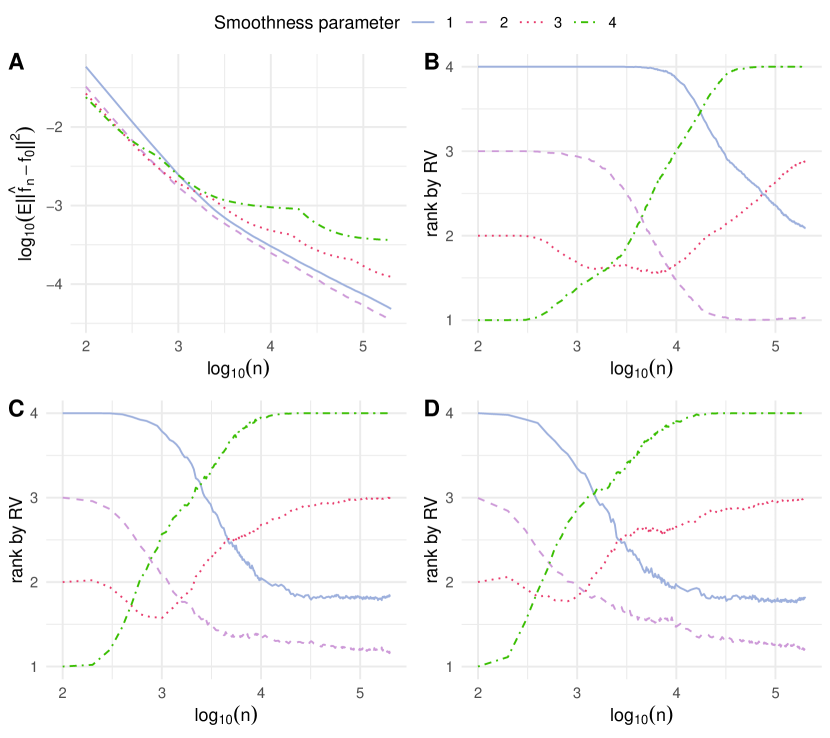
Figure 1: Model selection results of Example 6.1. (A) the (unavailable) true estimation errors of the candidate models; (B)-(D), average rankings of the models at different sample sizes over 500 repetitions, according to wRV, with weight exponent $\xi=0,1,2$, respectively.

Example 6.2 (Multivariate nonparametric regression).

We also include a set of simulation results of multivariate nonparametric online estimation. In this setting, we have

$$X_{i} \sim\mathcal{U}([0,1]^{10}),$$

$$\epsilon_{i} \sim\mathcal{N}(0,2^{2}),$$

$$f_{0}(X_{i}) =\sum_{j\text{ is odd }}\left\{0.5-\left|X_{i}[j]-0.5\right|\right\}+\sum_{j\text{ is even }}\exp\left(-X_{i}[j]\right),$$

$$Y_{i} =f_{0}\left(X_{i}\right)+\epsilon_{i}\,,$$

where the notation $X_{i}[j]$ means taking the $j$-th component of the $10$-dimensional vector $X_{i}$.

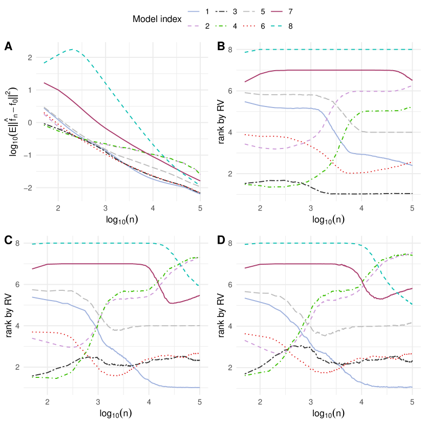
Figure 2: Model selection results of Example 2. $n$, number of samples processed by the estimators. (A) the (unavailable) true estimation errors of $8$ models; (B)-(D), average ranking of the models at different sample size, according to wRV. The RV weight exponents are $\xi=0,1,2$, respectively. Averaged over 500 repeats.

We compare eight different Sieve-SGD estimators that take different combinations of (1) assumed smoothness level $s\in\{1,2\}$; (2) initial step size $A\in\{0.1,1\}$ and (3) the initial number of basis functions $B\in\{2,8\}$. The definitions of these hyperparameters are given in (11), and see also the paragraph following equation (9). The exact model number and combination correspondence are given in Table 1 in Appendix F. The basis functions we use are products of univariate cosine functions: $\prod_{m=1}^{10}\cos((l[m]-1)\pi x[m])$ for some $l\in(\mathbb{N}^{+})^{10}$. In the univariate feature case, people almost always use the cosine basis of lower frequency first. However, in the multivariate case, there is no such ordering of the product basis functions. We reorder the multivariate cosine functions based on the product magnitude ($=\prod_{m=1}^{10}l[m]$) of the index vector $l$, in an increasing order. This way of reordering multivariate sieve basis functions can lead to rate-optimal estimators in certain tensor product Sobolev spaces [34].

The actual estimation errors (Panel A) and model selection frequencies (Panels BD̃) for this example are presented in Figure 2. According to Panel A, models 3 and 4 are better when sample size is less than $250$. As more samples are being processed, models 1, 3, and 6 perform better.

According to the unweighted RV statistics (Panel B), model 3 is always one of the best-performing ones (second place when $n<10^{2.7}$). This is consistent with the (unavailable) true estimation error in Panel A. The wRV statistics also captured the phenomenon that model 4 is better when the sample size is small but falls behind when the sample size is larger. If one observes Panel A closely, model 1 is narrowly the best one when $n>10^{3.5}$. Unfortunately, this small difference seems not fully captured by the unweighted RV in Panel B (model 1 does not frequently win the first place). This difficulty is overcome by weighted RV in Panels C and D. Model 1 becomes the preferred choice of wRV as the best when the sample size exceeds $10^{3.7}$ samples, and such selection becomes consistent when $n\geq 10^{4}$. Models $7$ and $8$ use a large initial learning rate and initial basis function number that result in a larger estimation error at an early stage—model $8$ even has an irregular increasing error. After a fast-improving stage, they eventually surpassed models $2$ and $4$ that performed well in the beginning. This feature is barely captured by unweighted RV at the sample size range considered here but is better reflected by weighted RV in panel D.

7 Discussion

The rolling validation method provides a computationally efficient way for online adaptive regression, with a theoretically justifiable performance guarantee under stability conditions. We analyze our method in the regression setting but the method and results can be extended to other nonparametric estimation tasks. For example, one can replace the squared loss with the “pinball” loss

$$l(f;X,Y):=\begin{cases}\alpha(Y-f(X))&\text{ if }Y>f(X)\\ (1-\alpha)(f(X)-Y)&\text{ otherwise }\end{cases}$$

to perform online adaptive quantile regression. In Figure 3 we demonstrate the $95\%$ and $5\%$ conditional quantile regression results (using Sieve-SGD). The hyperparameter is tuned by weighted RV with rolling weight exponent $\xi=1$. We also report the probability of the outcome lying between the regression curves.

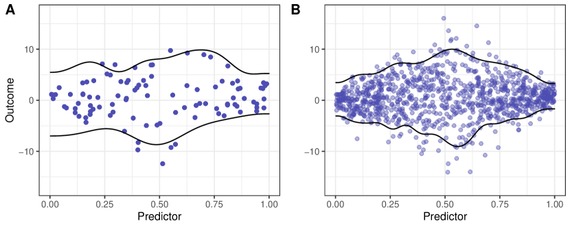
Figure 3: An example of applying weighted RV to quantile regression. The blue points represent training samples. (A) training sample size = 100. (B) training size increases to $10^{3}$, the blue points in (A) is a strict subset of those shown in (B). The estimators are trained in an online fashion using the same trajectory. The estimated coverage between the quantiles using a testing sample size $=10^{4}$ is (A) $91.7\%$ and (B) $90.6\%$.

So far we have been focusing on the scenario where the data points are generated from an unknown but not varying “true” distribution. However, the analysis framework presented in this paper can potentially be generalized to allow for time-varying distributions. One of the most interesting cases would be the true regression function experiencing certain “concept-drifts”: they may change abruptly at some time points or gradually over time. We expect some variants of the proposed weighted RV method can provide insights and practical tools in tracing the time-varying model selection target.

Appendix A Proof of Theorem 4.1

Proof.

We first present the proof of comparing two estimators that are different in convergence rates, that is, under the assumption that $a_{g}>a_{h}$. Denote $H_{n}=\sum_{i=1}^{n}i^{\xi}E\left\{h_{i-1}(X)-f_{0}(X)\right\}^{2}$. For any $\delta\in(0,1/4)$:

$$\operatorname{pr}(\text{ correct selection }) =\operatorname{pr}\left(\sum_{i=1}^{n}i^{\xi}\left\{h_{i-1}\left(X_{i}\right)-Y_{i}\right\}^{2}-i^{\xi}\epsilon_{i}^{2}\geq\sum_{i=1}^{n}i^{\xi}\left\{g_{i-1}\left(X_{i}\right)-Y_{i}\right\}^{2}-i^{\xi}\epsilon_{i}^{2}\right)$$ (36)

$$\geq\operatorname{pr}\left(\sum_{i=1}^{n}i^{\xi}\left\{h_{i-1}\left(X_{i}\right)-Y_{i}\right\}^{2}-i^{\xi}\epsilon_{i}^{2}\geq(1-\delta)H_{n}\right.\text{ and }$$

$$\left.\sum_{i=1}^{n}i^{\xi}\left\{g_{i-1}\left(X_{i}\right)-Y_{i}\right\}^{2}-i^{\xi}\epsilon_{i}^{2}\leq(1-\delta)H_{n}\right)$$

$$=1-\operatorname{pr}\left(\sum_{i=1}^{n}i^{\xi}\left\{h_{i-1}\left(X_{i}\right)-Y_{i}\right\}^{2}-i^{\xi}\epsilon_{i}^{2}\leq(1-\delta)H_{n}\right.\text{ or }$$

$$\quad\left.\sum_{i=1}^{n}i^{\xi}\left\{g_{i-1}\left(X_{i}\right)-Y_{i}\right\}^{2}-i^{\xi}\epsilon_{i}^{2}\geq(1-\delta)H_{n}\right)$$

$$\geq 1-\operatorname{pr}\left(\sum_{i=1}^{n}i^{\xi}\left\{h_{i-1}\left(X_{i}\right)-Y_{i}\right\}^{2}-i^{\xi}\epsilon_{i}^{2}\leq(1-\delta)H_{n}\right)$$

$$\quad-\operatorname{pr}\left(\sum_{i=1}^{n}i^{\xi}\left\{g_{i-1}\left(X_{i}\right)-Y_{i}\right\}^{2}-i^{\xi}\epsilon_{i}^{2}\geq(1-\delta)H_{n}\right)$$

Applying Corollary 4.5, we can verify that the probabilities in the last line converges to zero under the Theorem’s assumptions. For the first probability, we have:

$$\operatorname{pr}\left(\sum_{i=1}^{n}i^{\xi}\left\{h_{i-1}\left(X_{i}\right)-Y_{i}\right\}^{2}-i^{\xi}\epsilon_{i}^{2}\leq(1-\delta)H_{n}\right)$$ (37)

$$\leq\operatorname{pr}\left(\left|\sum_{i=1}^{n}i^{\xi}\left\{h_{i-1}\left(X_{i}\right)-Y_{i}\right\}^{2}-i^{\xi}\epsilon_{i}^{2}-H_{n}\right|\geq\delta H_{n}\right)$$

$$\stackrel{{\scriptstyle(I)}}{{\leq}}\operatorname{pr}\left(\left|\sum_{i=1}^{n}i^{\xi}\left\{h_{i-1}\left(X_{i}\right)-Y_{i}\right\}^{2}-i^{\xi}\epsilon_{i}^{2}-H_{n}\right|\geq\delta n^{1-a_{h}+\xi}\tilde{M}_{h}/2\right)$$

$$\text{ (for large }n\text{ such that }\left|n^{a_{h}-\xi-1}H_{n}-\tilde{M}_{h}\right|\leq\tilde{M}_{h}/2\text{ ) }$$

In step $(I)$ we used the fact that (it can be proved using the definition of limit, see an example in Lemma A.1):

$$\lim_{i\rightarrow\infty}i^{a_{h}}E\left\{h_{i-1}(X)-f_{0}(X)\right\}^{2} =M_{h}$$ (38)

$$\Rightarrow\lim_{n\rightarrow\infty}n^{a_{h}-1-\xi}\sum_{i=1}^{n}i^{\xi}E\left\{h_{i-1}(X)-f_{0}(X)\right\}^{2} =M_{h}/(1+\xi-a_{h})=:\tilde{M}_{h}$$

Then we can apply Corollary 4.5 to show the last line of (37) converging to zero as $n\rightarrow\infty$.

To bound $\operatorname{pr}\left(\sum_{i=1}^{n}i^{\xi}\left\{g_{i-1}\left(X_{i}\right)-Y_{i}\right\}^{2}-i^{\xi}\epsilon_{i}^{2}\geq(1-\delta)H_{n}\right)$, we denote $G_{n}=\sum_{i=1}^{n}i^{\xi}E\left\{g_{i-1}(X)-f_{0}(X)\right\}^{2}$. Then we have:

$$\operatorname{pr}\left(\sum_{i=1}^{n}i^{\xi}\left\{g_{i-1}\left(X_{i}\right)-Y_{i}\right\}^{2}-i^{\xi}\epsilon_{i}^{2}\geq(1-\delta)H_{n}\right)$$ (39)

$$\stackrel{{\scriptstyle(I)}}{{=}}\operatorname{pr}\left(\sum_{i=1}^{n}i^{\xi}\left\{g_{i-1}\left(X_{i}\right)-Y_{i}\right\}^{2}-i^{\xi}\epsilon_{i}^{2}-G_{n}\geq(1-\delta)H_{n}-G_{n}\right)$$

(for large $$n G_{n}<(1-\delta)H_{n}$$ such that )

$$\stackrel{{\scriptstyle(II)}}{{\leq}}\operatorname{pr}\left(\sum_{i=1}^{n}i^{\xi}\left\{g_{i-1}\left(X_{i}\right)-Y_{i}\right\}^{2}-i^{\xi}\epsilon_{i}^{2}-G_{n}\geq(1-2\delta)H_{n}\right)$$

(for large $$n G_{n}<\min\{\delta H_{n},(1-\delta)H_{n}\}=\delta H_{n} \delta<1/4$$ such that , since )

$$\stackrel{{\scriptstyle(III)}}{{\leq}}\operatorname{pr}\left(\sum_{i=1}^{n}i^{\xi}\left\{g_{i-1}\left(X_{i}\right)-Y_{i}\right\}^{2}-i^{\xi}\epsilon_{i}^{2}-G_{n}\geq(1-2\delta)n^{1-a_{h}+\xi}\tilde{M}_{h}/2\right)$$

(for large $$n G_{n}<\delta H_{n} |n^{a_{h}-\xi-1}H_{n}-\tilde{M}_{h}|\leq\tilde{M}_{h}/2$$ such that and )

In step $(I),(II)$ we used $H_{n}$ is a positive sequence diverging in a faster rate than $G_{n}$ (by our assumption that $a_{g}>a_{h}$). In step $(III)$ we used (38) again. Under the conditions on the convergence rate and estimator stability, we can verify that $c_{n}=(1-2\delta)n^{1-a_{h}+\xi}\tilde{M}_{h}/2$ satisfies the requirement in (27). Therefore the above deviation probability converges to $0$ according to Corollary 4.5.

In the case that $a_{g}=a_{h}$ but the constants differ $M_{g}<M_{h}$, the proof is very similar. The only twist is that we cannot pick any $\delta\in(0,1/4)$ as above. Instead, we should more carefully choose $\delta\in(0,1-(M_{g}/M_{h})^{1/3})$. We keep the same argument in (36) and (37), but modify (39) as:

$$\operatorname{pr}\left(\sum_{i=1}^{n}i^{\xi}\left\{g_{i-1}\left(X_{i}\right)-Y_{i}\right\}^{2}-i^{\xi}\epsilon_{i}^{2}\geq(1-\delta)H_{n}\right)$$ (40)

$$\leq\operatorname{pr}\left(\sum_{i=1}^{n}i^{\xi}\left\{g_{i-1}\left(X_{i}\right)-Y_{i}\right\}^{2}-i^{\xi}\epsilon_{i}^{2}\geq(1-\delta)^{2}n^{1-a_{h}+\xi}\tilde{M}_{h}\right)$$

(for large $$n \left|n^{a_{h}-\xi-1}H_{n}-\tilde{M}_{h}\right|\leq\delta\tilde{M}_{h}$$ such that )

$$\stackrel{{\scriptstyle(IV)}}{{\leq}}\operatorname{pr}\left(\sum_{i=1}^{n}i^{\xi}\left\{g_{i-1}\left(X_{i}\right)-Y_{i}\right\}^{2}-i^{\xi}\epsilon_{i}^{2}-G_{n}\geq(1-\delta)^{2}n^{1-a_{h}+\xi}\tilde{M}_{h}-G_{n}\right)$$

(for large $$n \left|n^{a_{h}-\xi-1}H_{n}-\tilde{M}_{h}\right|\leq\delta\tilde{M}_{h} G_{n}\leq(1-\delta)^{3}n^{1-a_{h}+\xi}\tilde{M}_{h}$$ such that and )

$$\leq\operatorname{pr}\left(\sum_{i=1}^{n}i^{\xi}\left\{g_{i-1}\left(X_{i}\right)-Y_{i}\right\}^{2}-i^{\xi}\epsilon_{i}^{2}-G_{n}\geq\delta(1-\delta)^{2}n^{1-a_{h}+\xi}\tilde{M}_{h}\right)$$

(for large $$n \left|n^{a_{h}-\xi-1}H_{n}-\tilde{M}_{h}\right|\leq\delta\tilde{M}_{h} G_{n}\leq(1-\delta)^{3}n^{1-a_{h}+\xi}\tilde{M}_{h}$$ such that and )

In step $(IV)$, it is possible to find large enough $n$ such that $G_{n}\leq(1-\delta)^{3}n^{1-a_{h}+\xi}\tilde{M}_{h}$. In fact, similar to $H_{n}$, we also have (recall $a_{g}=a_{h}$):

$$\lim_{n\rightarrow\infty}n^{a_{h}-1-\xi}\sum_{i=1}^{n}i^{\xi}E\left\{g_{i-1}(X)-f_{0}(X)\right\}^{2}=M_{g}/\left(1+\xi-a_{h}\right)=:\tilde{M}_{g}.$$ (41)

This means we can find large enough $n$ such that

$$G_{n}\leq(\tilde{M}_{g}+\epsilon)n^{1+\xi-a_{h}}\text{ for any }\epsilon>0.$$ (42)

Specifically, we can take $\epsilon=(1-\delta)^{3}\tilde{M}_{h}-\tilde{M}_{g}$ (Due to our choice of $\delta\in\left(0,1-\left(M_{g}/M_{h}\right)^{1/3}\right)$, this is indeed a positive number). The last line of (40) can be bounded using Corollary 4.5. ∎

Lemma A.1.

Suppose for a bounded positive sequence $\{h_{i},i=1,2,...\}$ we have

$$\lim_{i\rightarrow\infty}i^{a}h_{i}=M,$$ (43)

for some $a\in(0,1),M>0$. Then for any $\xi\geq 0$, we have

$$\lim_{n\rightarrow\infty}n^{a-\xi-1}\sum_{i=1}^{n}i^{\xi}h_{i}=M/(1+\xi-a)=:\tilde{M}.$$ (44)

Proof.

By definition of limit, we have: for any $\epsilon_{1}>0$, there exists some $N_{1}$ such that for any $i\geq N_{1}$:

$$|i^{a}h_{i}-M|\leq\epsilon_{1}.$$ (45)

We want to show that for any $\epsilon_{2}>0$, there exists some $N_{2}$ such that for any $n\geq N_{2}$:

$$\left|n^{a-\xi-1}\sum_{i=1}^{n}i^{\xi}h_{i}-\tilde{M}\right|\leq\epsilon_{2}$$ (46)

We show the details of upper bounding $n^{a-\xi-1}\sum_{i=1}^{n}i^{\xi}h_{i}-\tilde{M}$:

$$n^{a-\xi-1}\sum_{i=1}^{n}i^{\xi}h_{i}-\tilde{M}$$ (47)

$$\leq n^{a-\xi-1}\{\sum_{i=1}^{N_{1}}i^{\xi}h_{i}+\sum_{i=N_{1}+1}^{n}i^{\xi}(M+\epsilon_{1})i^{-a}\}-\tilde{M}$$

$$=n^{a-\xi-1}\sum_{i=1}^{N_{1}}i^{\xi}h_{i}+n^{a-\xi-1}(M+\epsilon_{1})\sum_{i=N_{1}+1}^{n}i^{\xi-a}-\tilde{M}$$

The term $n^{a-\xi-1}\sum_{i=1}^{N_{1}}i^{\xi}h_{i}$ above can be arbitrarily small as $n\rightarrow\infty$ since $h_{i}$ is uniformly bounded.

When $\xi-a>0$ (the other cases can be done similarly):

$$\sum_{i=N_{1}+1}^{n}i^{\xi-a}\leq\int_{N_{1}+1}^{n+1}x^{\xi-a}dx\leq(1+\xi-a)^{-1}(n+1)^{1+\xi-a},$$ (48)

then

$$n^{a-\xi-1}\left(M+\epsilon_{1}\right)\sum_{i=N_{1}+1}^{n}i^{\xi-a}\leq\frac{M+\epsilon_{1}}{1+\xi-a}\left(\frac{n+1}{n}\right)^{1+\xi-a}$$ (49)

$$\Rightarrow n^{a-\xi-1}\left(M+\epsilon_{1}\right)\sum_{i=N_{1}+1}^{n}i^{\xi-a}-\tilde{M}\leq\frac{M+\epsilon_{1}}{1+\xi-a}\left(\frac{n+1}{n}\right)^{1+\xi-a}-\tilde{M}$$

Since $\left(\frac{n+1}{n}\right)^{1+\xi-a}$ converges to $1$, (49) can also be arbitrarily small. ∎

Appendix B Proof of Lemma 4.2

Proof.

All we need is Chebyshev’s inequality ($u_{i}$ is defined in (22)):

$$\operatorname{pr}\left(\left|\sum_{i=1}^{n}i^{\xi}\epsilon_{i}\left\{\hat{f}_{i-1}\left(X_{i}\right)-f_{0}\left(X_{i}\right)\right\}\right|\geq c_{n}\right)\leq 2c_{n}^{-2}\text{var}\left(\sum_{i=1}^{n}i^{\xi}\epsilon_{i}\left\{\hat{f}_{i-1}\left(X_{i}\right)-f_{0}\left(X_{i}\right)\right\}\right)$$

$$=2c_{n}^{-2}\left(\sum_{i=1}^{n}\text{var}[i^{\xi}\epsilon_{i}\{\hat{f}_{i-1}(X_{i})-f_{0}(X_{i})\}]+\sum_{i\neq j}\text{cov}[i^{\xi}\epsilon_{i}\{\hat{f}_{i-1}(X_{i})-f_{0}(X_{i})\},j^{\xi}\epsilon_{j}\{\hat{f}_{j-1}(X_{j})-f_{0}(X_{j})\}]\right)$$

$$\stackrel{{\scriptstyle(I)}}{{=}}2c_{n}^{-2}\sum_{i=1}^{n}i^{2\xi}E[\epsilon_{i}^{2}u_{i}]\leq 2\sigma^{2}c_{n}^{-2}\sum_{i=1}^{n}i^{2\xi}E[u_{i}]\stackrel{{\scriptstyle(II)}}{{\rightarrow}}0$$

In step $(I)$ we used the noise variables $\epsilon_{i}$ are centered and independent from each other. Recall $\sigma^{2}$ is the bound on the variance of $\epsilon_{i}$ (conditioned on $X_{i}$). For step $(II)$ we combined condition (A2) and the assumption on sequence $c_{n}$. ∎

Appendix C Proof of Lemma 4.3

Proof.

Denote $Z_{i}=u_{i}-E[u_{i}\mid F^{i-1}]$, we have $E[Z_{i}]=E[Z_{i}\mid F^{i-1}]=0$. Then applying Chebyshev’s inequality:

$$\operatorname{pr}\left(\left|\sum_{i=1}^{n}Z_{i}\right|\geq c_{n}\right) \leq 2c_{n}^{-2}\operatorname{var}\left(\sum_{i=1}^{n}Z_{i}\right)$$ (50)

$$=2c_{n}^{-2}E\left(\sum_{i=1}^{n}Z_{i}\right)^{2}$$

$$=2c_{n}^{-2}\left\{\sum_{i=1}^{n}EZ_{i}^{2}+\sum_{i\neq j}E[Z_{i}Z_{j}]\right\}$$

Note that, for $j\leq i-1$:

$$E[Z_{i}Z_{j}]=E[Z_{j}E[Z_{i}|F^{j}]]=0$$ (51)

So we have

$$\operatorname{pr}\left(\left|\sum_{i=1}^{n}Z_{i}\right|\geq c_{n}\right) \leq 2c_{n}^{-2}\sum_{i=1}^{n}EZ_{i}^{2}=2c_{n}^{-2}\sum_{i=1}^{n}E\left(u_{i}-E\left[u_{i}\mid F^{i-1}\right]\right)^{2}$$ (52)

$$=2c_{n}^{-2}\sum_{i=1}^{n}Eu_{i}^{2}+E[E^{2}[u_{i}\mid F^{i-1}]]-2E[u_{i}E[u_{i}\mid F^{i-1}]]$$

$$\leq 2c_{n}^{-2}\sum_{i=1}^{n}Eu_{i}^{2}=2c_{n}^{-2}\sum_{i=1}^{n}i^{2\xi}E\left[\left\{\hat{f}_{i-1}\left(X_{i}\right)-f_{0}\left(X_{i}\right)\right\}^{4}\right]\stackrel{{\scriptstyle(I)}}{{\rightarrow}}0$$

In step $(I)$ we used condition A2 and our assumption on sequence $c_{n}$. ∎

Appendix D Proof of Lemma 4.4

Proof.

We will show that

$$c_{n}^{-1}\left|\sum_{i=1}^{n}E[u_{i}|F^{i-1}]-E[u_{i}]\right|\rightarrow 0\text{ in probability,}$$ (53)

which is implied by

$$Ec_{n}^{-2}\left|\sum_{i=1}^{n}E[u_{i}|F^{i-1}]-E[u_{i}]\right|^{2}\rightarrow 0\,,$$ (54)

or equivalently

$$c_{n}^{-1}\left\|\sum_{i=1}^{n}E[u_{i}|F^{i-1}]-\sum_{i=1}^{n}E[u_{i}]\right\|_{2}=c_{n}^{-1}\left(E\left|\sum_{i=1}^{n}E[u_{i}|F^{i-1}]-\sum_{i=1}^{n}E[u_{i}]\right|^{2}\right)^{1/2}\rightarrow 0$$ (55)

We rearrange the terms on the left-hand-side of (55):

$$\left\|\sum_{i=1}^{n}E[u_{i}|F^{i-1}]-\sum_{i=1}^{n}E[u_{i}]\right\|_{2}^{2}$$

$$= \left\|\sum_{i=1}^{n}\left(E[u_{i}|F^{i-1}]-E[u_{i}|F^{i-2}]+E[u_{i}|F^{i-2}]-E[u_{i}|F^{i-3}]+\cdot\cdot\cdot+E[u_{i}|F^{1}]-E[u_{i}]\right)\right\|_{2}^{2}$$

$$= \left\|\sum_{i=1}^{n}\sum_{j=1}^{i-1}E\left[u_{i}\mid F^{j}\right]-E\left[u_{i}\mid F^{j-1}\right]\right\|_{2}^{2}$$

$$= \left\|\sum_{j=1}^{n-1}\sum_{i=j+1}^{n}E\left[u_{i}\mid F^{j}\right]-E\left[u_{i}\mid F^{j-1}\right]\right\|_{2}^{2}$$

$$\stackrel{{\scriptstyle(I)}}{{=}} \sum_{j=1}^{n-1}\left\|\sum_{i=j+1}^{n}E[u_{i}|F^{j}]-E[u_{i}|F^{j-1}]\right\|_{2}^{2}$$

$$\stackrel{{\scriptstyle(II)}}{{=}} \sum_{j=1}^{n-1}\left\|\sum_{i=j+1}^{n}E[\nabla_{j}u_{i}|F^{j}]\right\|_{2}^{2}\stackrel{{\scriptstyle(III)}}{{\leq}}\sum_{j=1}^{n-1}\left(\sum_{i=j+1}^{n}\|E[\nabla_{j}u_{i}|F^{j}]\|_{2}\right)^{2}\,.$$ (56)

In step $(I)$ we used that $M_{j}=\sum_{i=j+1}^{n}E[u_{i}|F^{j}]-E[u_{i}|F^{j-1}]$ is a martingale-difference sequence w.r.t. to the filtration $F^{j}$. Therefore $E[M_{l}M_{k}]=0$ for all $l\neq k$. In step $(II)$ we used the definition of the difference operator $\nabla_{j}$ and realize that $E(u_{i}(Z_{i})|F^{j-1})=E(u_{i}(Z_{i}^{j})|F^{j})$. where $Z_{i}=\{(X_{1},Y_{1}),...,(X_{i},Y_{i})\}$ and $Z_{i}^{j}$ is replacing the $j$-th component of $Z_{i}$ with an IID copy. Step $(III)$ is triangule inequality.

Now we look at the scale of each term in the summation above. We will need the following decomposition of the stability of the loss function:

$$i^{-\xi}\nabla_{j}u_{i}$$

$$= \nabla_{j}\{\hat{f}_{i-1}(X_{i})-f_{0}(X_{i})\}^{2}$$

$$= \{\hat{f}_{i-1}(X_{i};Z_{i-1})-f_{0}(X_{i})\}^{2}-\{\hat{f}_{i-1}(X_{i};Z_{i-1}^{j})-f_{0}(X_{i})\}^{2}$$

$$= \{\hat{f}_{i-1}(X_{i};Z_{i-1})-\hat{f}_{i-1}(X_{i};Z_{i-1}^{j})\}\{\hat{f}_{i-1}(X_{i};Z_{i-1})-f_{0}(X_{i})+\hat{f}_{i-1}(X_{i};Z_{i-1}^{j})-f_{0}(X_{i})\}$$

$$= \nabla_{j}\hat{f}_{i-1}(X_{i})\{\hat{f}_{i-1}(X_{i};Z_{i-1})-f_{0}(X_{i})+\hat{f}_{i-1}(X_{i};Z_{i-1}^{j})-f_{0}(X_{i})\}\,.$$ (57)

We use the shorter notation $\hat{f}_{i-1}^{(j)}(x)=\hat{f}(x;Z_{i-1}^{j})$. Then

$$E[\nabla_{j}u_{i}|F^{j}]$$

$$= i^{\xi}E[\{\nabla_{j}\hat{f}_{i-1}(X_{i})\}\{\hat{f}_{i-1}(X_{i})-f_{0}(X_{i})+\hat{f}_{i-1}^{(j)}(X_{i})-f_{0}(X_{i})\}|F^{j}]$$

$$\leq i^{\xi}\sqrt{E[\{\nabla_{j}\hat{f}_{i-1}(X_{i})\}^{2}|F^{j}]}\sqrt{E[\{\hat{f}_{i-1}(X_{i})-f_{0}(X_{i})+\hat{f}_{i-1}^{(j)}(X_{i})-f_{0}(X_{i})\}^{2}|F^{j}]}\,.$$

Under our assumptions (A3) that $\sqrt{E[\{\nabla_{j}\hat{f}_{i-1}(X_{i})\}^{2}|F^{j}]}$ can be bounded by some $\Xi_{i}=D_{2}i^{-b}$ almost surely, we can continue (56) as following:

$$\sum_{i=j+1}^{n}\left\|E[\nabla_{j}u_{i}|F^{j}]\right\|_{2}$$

$$\leq \sum_{i=j+1}^{n}i^{\xi}\left\|\sqrt{E[\{\nabla_{j}\hat{f}_{i-1}(X_{i})\}^{2}|F^{j}]}\sqrt{E[\{\hat{f}_{i-1}(X_{i})-f_{0}(X_{i})+\hat{f}_{i-1}^{(j)}(X_{i})-f_{0}(X_{i})\}^{2}|F^{j}]}\right\|_{2}$$

$$\leq \sum_{i=j+1}^{n}i^{\xi}\Xi_{i}\left\|\sqrt{E[\{\hat{f}_{i-1}(X_{i})-f_{0}(X_{i})+\hat{f}_{i-1}^{(j)}(X_{i})-f_{0}(X_{i})\}^{2}|F^{j}]}\right\|_{2}$$

$$= \sum_{i=j+1}^{n}i^{\xi}\Xi_{i}\left\|\hat{f}_{i-1}\left(X_{i}\right)-f_{0}\left(X_{i}\right)+\hat{f}_{i-1}^{(j)}\left(X_{i}\right)-f_{0}\left(X_{i}\right)\right\|_{2}$$

$$\lesssim \sum_{i=j+1}^{n}i^{\xi}\Xi_{i}\left\|\hat{f}_{i-1}\left(X_{i}\right)-f_{0}\left(X_{i}\right)\right\|_{2}$$

Under the assumption $\|\hat{f}_{i-1}(X_{i})-f_{0}(X_{i})\|_{2}\lesssim Ci^{-a/2}$ for some $a\in(1/2,1]$, we can further simplify the above to be

$$\sum_{i=j+1}^{n}\left\|E[\nabla_{j}u_{i}|F^{j}]\right\|_{2}\lesssim\sum_{i=j+1}^{n}i^{-c},\text{ where }c:=(a/2+b-\xi)\,.$$

1. When $c>1$,

   $$\sum_{j=1}^{n-1}\left(\sum_{i=j+1}^{n}\left\|E[\nabla_{j}u_{i}|F^{j}]\right\|_{2}\right)^{2}\lesssim\sum_{j=1}^{n-1}(j^{1-c}-n^{1-c})^{2}\lesssim n^{3-2c}\vee\log n$$

   Plugging above into (56),

   $$c_{n}^{-1}\left\|\sum_{i=1}^{n}E[u_{i}|F^{i-1}]-\sum_{i=1}^{n}E[u_{i}]\right\|_{2}\lesssim c_{n}^{-1}n^{3/2-c}\vee c_{n}^{-1}\log^{1/2}n$$

   Under the assumptions of $c_{n}$, the RHS above converges to $0$ as $n\rightarrow\infty$.

2. When $c=1$, by definition of $c$, we have $a/2+b-\xi=1$. Our assumptions on $c_{n}$ are reduced to $\lim_{n}c_{n}^{-1}n^{1/2}\log n=0$. So in this case we have

   $$\sum_{j=1}^{n-1}\left(\sum_{i=j+1}^{n}\left\|E[\nabla_{j}u_{i}|F^{j}]\right\|_{2}\right)^{2}\lesssim\sum_{j=1}^{n-1}\log^{2}n\lesssim n\log^{2}n\,,$$

   and

   $$c_{n}^{-1}\left\|\sum_{i=1}^{n}E[u_{i}|F^{i-1}]-\sum_{i=1}^{n}E[u_{i}]\right\|_{2}\lesssim c_{n}^{-1}n^{1/2}\log n\rightarrow 0\text{ as }n\rightarrow\infty$$

3. When $c<1$, we have

   $$\sum_{j=1}^{n-1}\left(\sum_{i=j+1}^{n}\left\|E[\nabla_{j}u_{i}|F^{j}]\right\|_{2}\right)^{2}\lesssim\sum_{j=1}^{n-1}(n^{1-c}-j^{1-c})^{2}\lesssim n^{3-2c}$$

   Similar to the case 1, we have $c_{n}^{-1}\left\|\sum_{i=1}^{n}E[u_{i}|F^{i-1}]-\sum_{i=1}^{n}E[u_{i}]\right\|_{2}\rightarrow 0$ as $n\rightarrow\infty$. ∎

Appendix E Stability of SGD estimators

E.1 Proof of Theorem 5.1

Proof.

Recall the iteration formula of the model parameter:

$$\beta_{0} =0\in\mathbb{R}^{p}$$ (58)

$$\beta_{i} =\beta_{i-1}+\gamma\left(Y_{i}-X_{i}^{\top}\beta_{i-1}\right)X_{i}$$

$$=\gamma Y_{i}X_{i}+(I-\gamma X_{i}X_{i}^{\top})\beta_{i-1}$$

In our stability notation, $\beta_{i}$ can be written as $\beta_{i}(Z_{i})$, meaning it is calculated using the true sample $Z_{i}=\{(X_{1},Y_{1}),...,(X_{i},Y_{i})\}$. And we use $\beta^{\prime}_{i}=\beta^{\prime}_{i}(\nabla_{j}Z_{i})$ to denote the model parameter trained with sample $\nabla_{j}Z_{i}$, whose $j$-th sample is a IID copy of $(X_{j},Y_{j})$ in $Z_{i}$. We use $\eta_{i}$ to denote the difference between $\beta_{i}$ and $\beta^{\prime}_{i}$

$$\eta_{i}=\beta_{i}-\beta^{\prime}_{i}.$$ (59)

We are going to show $\eta_{i}$’s are vectors of small norm. It is trivial that $\eta_{i}=0$ when $j>i$ (the parameters are calculated using the same samples). When $i=j$,

$$\eta_{j}=\gamma Y_{i}X_{i}+\left(I-\gamma X_{i}X_{i}^{\top}\right)\beta_{i-1}-\gamma Y^{\prime}_{i}X^{\prime}_{i}+\left(I-\gamma X^{\prime}_{i}X_{i}^{\prime\top}\right)\beta_{i-1}$$ (60)

For $i\geq j+1$, we have the iteration formula:

$$\eta_{i} =(I-\gamma\|X_{i}\|^{2}H_{i})\eta_{i-1}$$ (61)

$$=H_{i}^{\perp}\eta_{i-1}+(1-\gamma\|X_{i}\|^{2})H_{i}\eta_{i-1},$$ (62)

where we used $H_{i}=X_{i}(\|X_{i}\|^{2})^{-1}X_{i}^{\top}$ to denote the projection matrix onto the direction of $X_{i}$ and $H_{i}^{\perp}=I-H_{i}$ is the projection onto its orthogonal complement.

Then we have

$$\|\eta_{i}\|^{2} =\|H_{i}^{\perp}\eta_{i-1}\|^{2}+(1-\gamma\|X_{i}\|^{2})^{2}\|H_{i}\eta_{i-1}\|^{2}$$ (63)

$$\stackrel{{\scriptstyle(I)}}{{\leq}}\|H_{i}^{\perp}\eta_{i-1}\|^{2}+(1-\gamma\|X_{i}\|^{2})\|H_{i}\eta_{i-1}\|^{2}$$ (64)

$$\leq\|\eta_{i-1}\|^{2}-\gamma\|X_{i}\|^{2}\|H_{i}\eta_{i-1}\|^{2}$$ (65)

In step $(I)$ we used $\gamma\|X_{i}\|^{2}\leq 1$. Therefore,

$$\frac{\|\eta_{i}\|^{2}}{\|\eta_{i-1}\|^{2}}\leq 1-\gamma\|X_{i}\|^{2}\frac{\|H_{i}\eta_{i-1}\|^{2}}{\|\eta_{i-1}\|^{2}}=1-\gamma\frac{\eta_{i-1}^{\top}X_{i}X_{i}^{\top}\eta_{i-1}}{\|\eta_{i-1}\|^{2}}$$ (66)

Take conditional expectation on both sides:

$$E\left[\left.\frac{\|\eta_{i}\|^{2}}{\|\eta_{i-1}\|^{2}}\right|F_{i-1}\right] \leq 1-\gamma\|\eta_{i-1}\|^{-2}\eta_{i-1}^{\top}E[X_{i}X_{i}^{\top}]\eta_{i-1}$$ (67)

$$\stackrel{{\scriptstyle(II)}}{{\leq}}1-\gamma\underline{\lambda}\leq\exp(-\gamma\underline{\lambda}).$$

In step $(II)$ we used the assumption that $\lambda_{min}(E[X_{i}X_{i}^{\top}])\geq\underline{\lambda}>0$. Now we established some “exponential contraction” properties for the sequence of vectors $\{\eta_{i}\}$. Then we can apply Lemma E.1 (with parameter $a$ therein equals to $0$) to conclude that the averaged coefficient vector $\hat{\eta}_{i}=i^{-1}\sum_{k=1}^{i}\eta_{k}$ has magnitude:

$$E[\|\hat{\eta}_{i}\|^{2}|F^{j}]\lesssim i^{-2}\|\eta_{j}\|^{2}$$ (68)

Recall that our goal is to control the stability of the estimator. Use the bound on $\hat{\eta}_{i}$ we have:

$$E\left[\left\{\nabla_{j}\hat{f}_{i-1}\left(X_{i}\right)\right\}^{2}\mid F^{j}\right] =E\left[\left\{\hat{f}_{i-1}\left(X_{i};Z_{i}\right)-\hat{f}_{i-1}\left(X_{i};\nabla_{j}Z_{i}\right)\right\}^{2}\mid F^{j}\right]$$ (69)

$$=E\left[\left\{X_{i}^{\top}\hat{\beta}_{i-1}-X_{i}^{\top}\hat{\beta}_{i-1}^{\prime}\right\}^{2}\mid F^{j}\right]$$

$$\text{ (where }\hat{\beta}_{i}=i^{-1}\sum_{k=1}^{i}\beta_{k},\ \hat{\beta}^{\prime}_{i}=i^{-1}\sum_{k=1}^{i}\beta^{\prime}_{k})$$

$$=E\left[\left.\{X_{i}^{\top}\hat{\eta}_{i-1}\}^{2}\right|F^{j}\right]$$

$$\leq E\left[\left.\|X_{i}\|^{2}\|\hat{\eta}_{i-1}\|^{2}\right|F^{j}\right],$$

Under the assumption that $E[\|X_{i}\|^{2}]\leq R^{2}$,

$$E\left[\left\{\nabla_{j}\hat{f}_{i-1}\left(X_{i}\right)\right\}^{2}\mid F^{j}\right] \leq R^{2}E\left[\left\|\hat{\eta}_{i-1}\right\|^{2}\mid F^{j}\right]$$ (70)

$$\stackrel{{\scriptstyle(III)}}{{\lesssim}}i^{-2}\|\eta_{j}\|^{2}$$

In step $(III)$ we used (68). Under the uniform assumptions: $\|X_{j}\|^{2}\leq R^{2}$ and $|Y_{j}-X_{j}^{\top}\beta_{j-1}|\leq M$, we have

$$\left\|\eta_{j}\right\| \leq\left\|\gamma X_{j}\left(Y_{j}-X_{j}^{\top}\beta_{j-1}\right)\right\|+\left\|\gamma X_{j}^{\prime}\left(Y_{j}^{\prime}-X_{j}^{\prime\top}\beta_{j-1}\right)\right\|$$ (71)

$$\leq 2\gamma MR$$

$$\Rightarrow\|\eta_{j}\|^{2} \leq 4\gamma^{2}M^{2}R^{2}.$$

Combine (70) and (71), we know

$$E\left[\left\{\nabla_{j}\hat{f}_{i-1}\left(X_{i}\right)\right\}^{2}\mid F^{j}\right]\lesssim i^{-2},$$ (72)

which concludes our proof.

∎

E.2 Proof of Theorem 5.2

Proof.

Let $\beta_{i}$ be the coefficient vectors trained with sample $Z_{i}=\left\{\left(X_{1},Y_{1}\right),\left(X_{2},Y_{2}\right),\ldots,\left(X_{j},Y_{j}\right),\ldots,\left(X_{i},Y_{i}\right)\right\}$ and $\beta_{i}^{\prime}$ be the coefficient vectors trained with sample $\nabla_{j}Z_{i}=\left\{\left(X_{1},Y_{1}\right),\left(X_{2},Y_{2}\right),\ldots,\left(X_{j}^{\prime},Y_{j}^{\prime}\right),\ldots,\left(X_{i},Y_{i}\right)\right\}$. The two sets of training samples are the same except for the $j$-th pair. Here we used $i\geq j$—for $i<j$ the two coefficient vectors are the same. At the $j$-th step, $\beta_{i}$ is updated using sample $\left(X_{j},Y_{j}\right)$:

$$\beta_{j}=\beta_{j-1}^{\wedge}+\gamma_{j}\left(Y_{j}-\bm{\phi}_{j}^{\top}\beta_{j-1}^{\wedge}\right)D_{j}\phi_{j},$$ (73)

And we have a similar updating rule for $\beta_{j}^{\prime}$ using sample $\left(X_{j}^{\prime},Y_{j}^{\prime}\right)$ :

$$\beta_{j}^{\prime} =\beta_{j-1}^{\prime\wedge}+\gamma_{j}\left(Y_{j}-\bm{\phi}_{j}^{\prime\top}\beta_{j-1}^{\prime\wedge}\right)D_{j}\bm{\phi}_{j}^{\prime}$$ (74)

$$=\beta_{j-1}^{\wedge}+\gamma_{j}\left(Y_{j}-\bm{\phi}_{j}^{\prime\top}\beta_{j-1}^{\wedge}\right)D_{j}\bm{\phi}_{j}^{\prime}$$

Here $\bm{\phi}_{j}^{\prime}=\left(\phi_{1}\left(X_{j}^{\prime}\right),\ldots,\phi_{J_{i}}\left(X_{j}^{\prime}\right)\right)^{\top}$.

Let $\eta_{i}=\beta_{i}-\beta_{i}^{\prime}$ be the difference between the two vectors. We have $\eta_{i}=0$ for $i<j$. And

$$\eta_{j}=\gamma_{j}\left(Y_{j}-\bm{\phi}_{j}^{\top}\beta_{j-1}^{\wedge}\right)D_{j}\bm{\phi}_{j}-\gamma_{j}\left(Y_{j}-\bm{\phi}_{j}^{\prime\top}\beta_{j-1}^{\prime\wedge}\right)D_{j}\bm{\phi}_{j}^{\prime}.$$ (75)

From the recursive formula of $\beta_{i},\beta^{\prime}_{i}$ we can also derive one for $\eta_{i}$:

$$\eta_{i}=\eta_{i-1}^{\wedge}-\gamma_{i}D_{i}\bm{\phi}_{i}\bm{\phi}_{i}^{\top}\eta_{i-1}^{\wedge}$$ (76)

Multiply $D_{i}^{-1/2}$ on both sides:

$$D_{i}^{-1/2}\eta_{i}^{\wedge}=D_{i}^{-1/2}\eta_{i-1}^{\wedge}-\gamma_{i}D_{i}^{1/2}\bm{\phi}_{i}\left(D_{i}^{1/2}\bm{\phi}_{i}\right)^{\top}D_{i}^{-1/2}\eta_{i-1}^{\wedge}$$ (77)

Denote $\theta_{i}=D_{i}^{-1/2}\eta_{i},W_{i}=D_{i}^{1/2}\bm{\phi}_{i}$, we rewrite the above equation as:

$$\theta_{i}=\theta^{\wedge}_{i-1}-\gamma_{i}W_{i}W_{i}^{\top}\theta^{\wedge}_{i-1}$$ (78)

For the rest of the proof, we aim to derive some bounds on $\|\theta_{i}\|^{2}$ (and their averaged version $\hat{\theta}_{i}=i^{-1}\sum_{k=1}^{i}\theta_{k}$).

For $\theta_{j}$ we have the following bound:

$$\left\|\theta_{j}\right\| =\left\|\gamma_{j}\left(Y_{j}-\bm{\phi}_{j}^{\top}\beta_{j-1}^{\wedge}\right)D_{j}^{1/2}\bm{\phi}_{j}-\gamma_{j}\left(Y_{j}-\bm{\phi}_{j}^{\prime\top}\beta_{j-1}^{\prime\wedge}\right)D_{j}^{1/2}\bm{\phi}_{j}^{\prime}\right\|$$ (79)

$$\leq M\gamma_{j}\left(\left\|D_{j}^{1/2}\bm{\phi}_{j}\right\|+\left\|D_{j}^{1/2}\bm{\phi}_{j}^{\prime}\right\|\right)\stackrel{{\scriptstyle(I)}}{{\lesssim}}\gamma_{j}$$

In step $(I)$ above we used the norm of $D_{j}^{1/2}\bm{\phi}_{j}$ is uniformly bounded:

$$\|D_{j}^{1/2}\bm{\phi}_{j}\|^{2}=\sum_{k=1}^{J(j)}(k^{-\omega}\phi_{k}(X_{j}))^{2}\leq C\sum_{k=1}^{\infty}k^{-2\omega}<\infty,$$ (80)

recall that $\omega>1/2$. Now we are going to use the iteration formula to derive bounds for $\|\theta_{i}\|,i>j$. Take inner product on both sides of (78):

$$\left\|\theta_{i}\right\|^{2} =\left\|\theta_{i-1}^{\wedge}\right\|^{2}+\gamma_{i}^{2}\left(\theta_{i-1}^{\wedge}\right)^{\top}W_{i}W_{i}^{\top}W_{i}W_{i}^{\top}\theta_{i-1}^{\wedge}-2\gamma_{i}\left(\theta_{i-1}^{\wedge}\right)^{\top}W_{i}W_{i}^{\top}\theta_{i-1}^{\wedge}$$ (81)

$$\stackrel{{\scriptstyle(II)}}{{\leq}}\left\|\theta^{\wedge}_{i-1}\right\|^{2}-\gamma_{i}\theta_{i-1}^{\wedge\top}W_{i}W_{i}^{\top}\theta^{\wedge}_{i-1}$$

In step $(II)$ above we used $\gamma_{i}\|W_{i}\|^{2}\leq 1$. Take conditional expectation

$$E[\|\theta_{i}\|^{2}|F^{i-1}] \leq\|\theta^{\wedge}_{i-1}\|^{2}-\gamma_{i}\theta_{i-1}^{{}^{\wedge}\top}E[W_{i}W_{i}^{\top}]\theta^{\wedge}_{i-1}$$ (82)

$$=\|\theta_{i-1}\|^{2}-\gamma_{i}\theta_{i-1}^{{}^{\wedge}\top}D_{i}^{1/2}E[\bm{\phi}_{i}\bm{\phi}_{i}^{\top}]D_{i}^{1/2}\theta^{\wedge}_{i-1}$$

Divide $\|\theta_{i-1}\|^{2}=\|\theta^{\wedge}_{i-1}\|^{2}$ on both sides:

$$E[\|\theta_{i}\|^{2}/\|\theta_{i-1}\|^{2}|F^{i-1}]\leq 1-\gamma_{i}\frac{\theta_{i-1}^{{}^{\wedge}\top}D_{i}^{1/2}E[\bm{\phi}_{i}\bm{\phi}_{i}^{\top}]D_{i}^{1/2}\theta^{\wedge}_{i-1}}{\|\theta^{\wedge}_{i-1}\|^{2}}$$ (83)

By our assumption, $\lambda_{min}(E[\bm{\phi}_{i}\bm{\phi}_{i}^{\top}])$ is strictly larger than a constant (we postpone the proof after equation (88)). Also note that $D_{i}^{1/2}=diag(1^{-\omega},...,J_{i}^{-\omega})$ has eigenvalues greater than $J_{i}^{-\omega}=i^{-\zeta\omega}$. So overall we have

$$\frac{\theta_{i-1}^{{}^{\wedge}\top}D_{i}^{1/2}E[\bm{\phi}_{i}\bm{\phi}_{i}^{\top}]D_{i}^{1/2}\theta^{\wedge}_{i-1}}{\|\theta^{\wedge}_{i-1}\|^{2}}\geq i^{-2\zeta\omega}.$$ (84)

Then we have a exponential contraction recursion:

$$E[\|\theta_{i}\|^{2}/\|\theta_{i-1}\|^{2}|F^{i-1}]\leq 1-\gamma_{i}i^{-2\zeta\omega}=1-i^{-2\zeta\omega-\zeta}\leq\exp(-i^{-\alpha}),$$ (85)

for the ease of notation we defined $\alpha=2\zeta\omega+\zeta$. Now we are ready to apply Lemma E.1 to bound the magnitude of $\hat{\theta}_{i}=i^{-1}\sum_{k=1}^{i}\theta_{k}^{\wedge}$ as:

$$E[\|\hat{\theta}_{i}\|^{2}|F^{j}]\lesssim i^{-2}j^{2\alpha}\|\theta_{j}\|^{2}$$ (86)

Plug this into (79), we get

$$E[\|\hat{\theta}_{i}\|^{2}|F^{j}]\lesssim i^{-2}j^{2\alpha-2\zeta}=i^{-2}j^{4\omega\zeta}$$ (87)

This implies the stability property of the sieve SGD estimator, let $\hat{\beta}_{i}=i^{-1}\sum_{k=1}^{i}\beta_{k}^{\wedge}$ denote the averaged coefficient vector ($\hat{\beta}_{i}^{\prime},\hat{\eta}_{i}$ are similarly defined):

$$E\left[\left\{\nabla_{j}\hat{f}_{i-1}\left(X_{i}\right)\right\}^{2}\mid F^{j}\right] =E\left[\left\{\hat{f}_{i-1}\left(X_{i};Z_{i}\right)-\hat{f}_{i-1}^{\prime}\left(X_{i};\nabla_{j}Z_{i}\right)\right\}^{2}\mid F^{j}\right]$$ (88)

$$=E\left[\left\{\left\langle\hat{\beta}_{i-1}^{\wedge},\bm{\phi}_{i}\right\rangle-\left\langle\hat{\beta}_{i-1}^{\prime\wedge},\bm{\phi}_{i}\right\rangle\right\}^{2}\mid F^{j}\right]$$

$$=E\left[\left(\hat{\eta}_{i-1}^{\wedge\top}\bm{\phi}_{i}\right)^{2}\mid F^{j}\right]$$

$$=E\left[\left(\hat{\theta}_{i-1}^{\wedge\top}W_{i}\right)^{2}\mid F^{j}\right]$$

$$=E\left[\hat{\theta}_{i-1}^{\top}E\left[W_{i}W_{i}^{\top}\right]\hat{\theta}_{i-1}\mid F^{j}\right]$$

$$\lesssim\lambda_{\max}\left(E\left[W_{i}W_{i}^{\top}\right]\right)i^{4\omega\zeta-2}$$

To finalize the proof, we just need to bound the minimal (maximal) eigenvalue of matrix $E[\bm{\phi}_{i}\bm{\phi}_{i}^{\top}]$ ($E[W_{i}W_{i}^{\top}]$). We denote the density of $X$ (with respect to the measure $\nu$) as $p_{X}$. By our assumption there exists some positive constants $\bar{p}_{X},\underline{p}_{X}$ such that $0<\underline{p}_{X}\leq p_{X}(x)\leq\bar{p}_{X}<\infty$. Let $v$ denote any eigenvector of $E[\bm{\phi}_{i}\bm{\phi}_{i}^{\top}]$, we have:

$$v^{\top}E[\bm{\phi}_{i}\bm{\phi}_{i}^{\top}]v=E\left[\left(\sum_{k=1}^{J_{i}}\phi_{k}(X_{i})v_{k}\right)^{2}\right]\geq\underline{p}_{X}\int\left(\sum_{k=1}^{J_{i}}\phi_{k}(X_{i})v_{k}\right)^{2}d\nu=\underline{p}_{X}\|v\|^{2}$$ (89)

So we know $\lambda_{min}(E[\bm{\phi}_{i}\bm{\phi}_{i}^{\top}])\geq\underline{p}_{X}$. Similarly, let $u$ denote any eigenvector of $E[W_{i}W_{i}^{\top}]$:

$$u^{\top}E[W_{i}W_{i}^{\top}]u=E\left[\left(\sum_{k=1}^{J_{i}}k^{-\omega}\phi_{k}(X_{i})u_{k}\right)^{2}\right]\leq\bar{p}_{X}\|u\|^{2}.$$ (90)

So we know $\lambda_{max}(E[W_{i}W_{i}^{\top}])\leq\bar{p}_{X}$. Combine these eigenvalue results with (88), we conclude that

$$E\left[\left\{\nabla_{j}\hat{f}_{i-1}\left(X_{i}\right)\right\}^{2}\mid F^{j}\right]\lesssim i^{4\omega\zeta-2}$$

.

∎

E.3 A Technical Lemma

The following lemma was used in the proof of the stability properties of SGD estimators.

Lemma E.1.

Let $\{\eta_{i},i=1,2,...\}$ be a sequence of real vectors. Assume that there exists some $j\in\{1,2,...\}$ and some $a\in[0,1),A>0$ such that:

• $\eta_{i}=0$ when $i=1,2,...,j-1$;

• For all $i\geq j$, the sequence satisfies the following step-wise “exponential contraction” condition:

  $$E[\|\eta_{i+1}\|^{2}/\|\eta_{i}\|^{2}|F^{i}] \leq\exp(-Ai^{-a}).$$ (91)

Then for $\hat{\eta}_{n}=n^{-1}\sum_{i=1}^{n}\eta^{\wedge}_{i}$, we have

$$n^{2}E[\|\hat{\eta}_{n}\|^{2}|F^{j}]\leq C(a,A)j^{2a}\|\eta_{j}\|^{2},$$ (92)

with some constant $C(a,A)$ depending on $a,A$.

Remark 5.

the $\eta_{i}$ vectors in Lemma E.1 may belong to the same real-vector space $\mathbb{R}^{J}$ for a fixed, positive integer $J$. It is also possible that they belong to vector spaces of different dimensions, that is, $\eta_{i}\in\mathbb{R}^{J_{i}}$ where $J_{i}$ is a sequence of positive integers. The latter case is especially important when we prove the stability of Sieve-type SGD estimators (Theorem 5.2). To accommodate the varying dimension case, we used the $\wedge$ sign when defining the average vector $\hat{\eta}_{n}$: for vectors of lower dimension, we need to embed them into the higher dimensions and fill the extra entries with $0$.

Proof.

Our readers can take $a=0$ for the first pass which alleviates the technical complexity. For the ease of notation, we use $E_{j}$ to denote the conditional expectation $E[\cdot|F^{j}]$.

By our assumption (91), we have that for any $k>i\geq j$:

$$E_{k-1}\left[\|\eta_{k}\|^{2}/\|\eta_{i}\|^{2}\right] =E_{k-1}\left[\frac{\|\eta_{k-1}\|^{2}}{\|\eta_{i}\|^{2}}\frac{\|\eta_{k}\|^{2}}{\|\eta_{k-1}\|^{2}}\right]=\frac{\|\eta_{k-1}\|^{2}}{\|\eta_{i}\|^{2}}E_{k-1}\left[\frac{\|\eta_{k}\|^{2}}{\|\eta_{k-1}\|^{2}}\right]$$ (93)

$$\leq\exp(-A(k-1)^{-a})\|\eta_{k-1}\|^{2}/\|\eta_{i}\|^{2}$$

Iterate the above argument we have:

$$E_{i}[\|\eta_{k}\|^{2}/\|\eta_{i}\|^{2}]\leq\exp\left(-A\sum_{l=i}^{k-1}l^{-a}\right)$$ (94)

Apply Jensen’s inequality, we also have:

$$E_{i}[\|\eta_{k}\|/\|\eta_{i}\|] \leq\sqrt{E_{i}[\|\eta_{k}\|^{2}/\|\eta_{i}\|^{2}]}\leq\exp\left(-A\sum_{l=i}^{k-1}l^{-a}/2\right)$$ (95)

$$\Rightarrow E_{i}[\|\eta_{k}\|] \leq\exp\left(-A\sum_{l=i}^{k-1}l^{-a}/2\right)\|\eta_{i}\|$$

Expand the quantity of interest and plug in the above iteration equations we can derive our results:

$$n^{2}E_{j}[\|\hat{\eta}_{n}\|^{2}] =E_{j}\left[\left\|\sum_{i=j}^{n}\eta_{i}\right\|^{2}\right]\quad\text{ ($\eta_{i}=0$ for $i<j$)}$$ (96)

$$\leq 2\sum_{i=j}^{n}\sum_{k=i}^{n}E_{j}[\eta_{k}^{\top}\eta_{i}]$$

$$\leq 2\sum_{i=j}^{n}\sum_{k=i}^{n}E_{j}[\|\eta_{k}\|\|\eta_{i}\|]$$

$$\leq 2\sum_{i=j}^{n}\sum_{k=i}^{n}\exp\left(-A\sum_{l=i}^{k-1}l^{-a}/2\right)E_{j}[\|\eta_{i}\|^{2}]$$

$$\stackrel{{\scriptstyle(I)}}{{\leq}}C(a,A)\sum_{i=j}^{n}i^{a}E_{j}[\|\eta_{i}\|^{2}]$$

$$\leq C(a,A)\sum_{i=j}^{n}i^{a}\exp\left(-\sum_{l=j}^{i-1}l^{-a}\right)\|\eta_{j}\|^{2}$$

$$\stackrel{{\scriptstyle(II)}}{{\leq}}C(a,A)j^{2a}\|\eta_{j}\|^{2}$$

Step $(I)$ and $(II)$ are technical, we will present them below.

For step $(I)$, we need to show $\sum_{k=i}^{n}\exp(-\sum_{l=i}^{k-1}Al^{-a})\leq C(a,A)i^{a}$. Each term in the summation has the following bound:

$$\exp\left(-\sum_{l=i}^{k-1}Al^{-a}\right)\leq\exp(-A(1-a)^{-1}\{(k-1)^{1-a}-i^{1-a}\})$$ (97)

Then we have

$$\sum_{k=i}^{n}\exp\left(-\sum_{l=i}^{k-1}Al^{-a}\right) \leq\exp(A(1-a)^{-1}i^{1-a})\sum_{k=i}^{n}\exp(-A(1-a)^{-1}(k-1)^{1-a})$$ (98)

$$\leq\exp(A(1-a)^{-1}i^{1-a})\int_{i}^{n+1}\exp(-A(1-a)^{-1}(k-1)^{1-a})dk$$

Define $u=A(1-a)^{-1}(k-1)^{1-a}$, we have $du=A(k-1)^{-a}dk$ and $(k-1)^{-a}=\{A^{-1}(1-a)u\}^{-a/(1-a)}$. Therefore,

$$du =A\{A^{-1}(1-a)u\}^{-a/(1-a)}dk$$ (99)

$$\Rightarrow dk =A^{-1}\{A^{-1}(1-a)u\}^{a/(1-a)}du$$

Make the change of variable in (98), we simplify the integral as

$$\int_{A(1-a)^{-1}(i-1)^{1-a}}^{A(1-a)^{-1}n^{1-a}}\exp(-u)A^{-1}\{A^{-1}(1-a)u\}^{a/(1-a)}du$$ (100)

Note that the above integral is essentially the upper incomplete gamma function. We have the following upper bound of its magnitude:

Lemma E.2.

(Theorem 4.4.3 of [11]) Let $\Gamma(m,x)$ denote the upper incomplete gamma function:

$$\Gamma(m,x)=\int_{x}^{\infty}\exp(-u)u^{m-1}du,$$ (101)

with $x>m\geq 1$, then we have the upper bound

$$\Gamma(m,x)\leq m\exp(-x)x^{m-1}.$$ (102)

Applying Lemma E.2, we can continue (100) as:

$$\int_{i}^{n+1}\exp(-A(1-a)^{-1}k^{1-a})dk$$ (103)

$$\leq A^{-1-a/(1-a)}(1-a)^{a/(1-a)}\Gamma((1-a)^{-1},A(1-a)^{-1}(i-1)^{1-a})$$

$$\leq A^{-1-a/(1-a)}(1-a)^{a/(1-a)-1}\exp(-A(1-a)^{-1}(i-1)^{1-a})(A(1-a)^{-1}(i-1)^{1-a})^{a/(1-a)}$$

$$\leq A^{-1}(1-a)^{-1}\exp(-A(1-a)^{-1}(i-1)^{1-a})i^{a}$$

Combine (98) and (LABEL:good_term), we conclude the proof of step $(I)$ in (96).

The step $(II)$ of (96) can be shown using a similar argument.

$$\sum_{i=j}^{n}i^{a}\exp\left(-\sum_{l=j}^{i-1}Al^{-a}\right) \leq\exp(A(1-a)^{-1}j^{1-a})\sum_{i=j}^{n}\exp(-A(1-a)^{-1}(i-1)^{1-a})i^{a}$$ (104)

$$\leq\exp(A(1-a)^{-1}j^{1-a})\int_{j}^{n+1}\exp(-A(1-a)^{-1}(i-1)^{1-a})i^{a}di$$

Change the variable in the integral: $u=A(1-a)^{-1}(i-1)^{1-a}$, $du=A(i-1)^{-a}di$, $di=A^{-1}\{A^{-1}(1-a)u\}^{a/(1-a)}du$, so we can bound the integral in (104) by

$$\int_{A(1-a)^{-1}(j-1)^{1-a}}^{\infty}\exp(-u)i^{a}\{(1-a)u\}^{a/(1-a)}du$$ (105)

$$\leq 2^{a}A^{-1-2a/(1-a)}(1-a)^{2a/(1-a)}\int_{A(1-a)^{-1}(j-1)^{1-a}}^{\infty}\exp(-u)u^{2a/(1-a)}du$$

$$=2^{a}A^{-1-2a/(1-a)}(1-a)^{2a/(1-a)}\Gamma((1+a)/(1-a),A(1-a)^{-1}(j-1)^{1-a})$$

$$\leq 2^{a}A^{-1-2a/(1-a)}(1-a)^{2a/(1-a)}(1+a)/(1-a)$$

$$\qquad\exp(-A(1-a)^{-1}(j-1)^{1-a})\{A(1-a)^{-1}(j-1)^{1-a}\}^{2a/(1-a)}$$

$$\leq 2^{a}A^{-1}(1+a)(1-a)^{-1}\exp(-A(1-a)^{-1}(j-1)^{1-a})j^{2a}$$

∎

Appendix F More Details of the Numerical Study

In Section 6, example 2, we described performing model selection among $8$ sieve-SGD estimators. Here we list their hyperparameters. Recall that $\gamma_{i}=Ai^{-(2s+1)^{-1}}$ is the learning rate and $J_{i}=Bi^{(2s+1)^{-1}}$ is the number of basis function, as defined in (11). For all eight methods, $\omega$ in (9) is 0.51.

Model Index	$s$	$A$	$B$
1	1	0.1	2
2	2	0.1	2
3	1	1	2
4	2	1	2
5	1	0.1	8
6	2	0.1	8
7	1	1	8
8	2	1	8

Table 1: Hyperparameter for the estimators of example 2.

References

• Arlot and Celisse [2010] Arlot, S. and A. Celisse (2010). A survey of cross-validation procedures for model selection.
• Armstrong and Grohman [1972] Armstrong, J. S. and M. C. Grohman (1972). A comparative study of methods for long-range market forecasting. Management Science 19(2), 211–221.
• Bach and Moulines [2013] Bach, F. and E. Moulines (2013). Non-strongly-convex smooth stochastic approximation with convergence rate o (1/n). Advances in neural information processing systems 26.
• Benkeser et al. [2018] Benkeser, D., C. Ju, S. Lendle, and M. van der Laan (2018). Online cross-validation-based ensemble learning. Statistics in medicine 37(2), 249–260.
• Bousquet and Elisseeff [2002] Bousquet, O. and A. Elisseeff (2002). Stability and generalization. The Journal of Machine Learning Research 2, 499–526.
• Browne [2000] Browne, M. W. (2000). Cross-validation methods. Journal of mathematical psychology 44(1), 108–132.
• Calandriello et al. [2017] Calandriello, D., A. Lazaric, and M. Valko (2017). Efficient second-order online kernel learning with adaptive embedding. Advances in Neural Information Processing Systems 30.
• Dieuleveut and Bach [2016] Dieuleveut, A. and F. Bach (2016). Nonparametric stochastic approximation with large step-sizes.
• Ding et al. [2018] Ding, J., V. Tarokh, and Y. Yang (2018). Model selection techniques: An overview. IEEE Signal Processing Magazine 35(6), 16–34.
• Efron and Tibshirani [1997] Efron, B. and R. Tibshirani (1997). Improvements on cross-validation: the $.632+$ bootstrap method. Journal of the American Statistical Association 92(438), 548–560.
• Gabcke [1979] Gabcke, W. (1979). Neue Herleitung und explizite Restabschätzung der Riemann-Siegel-Formel. Ph. D. thesis, Georg-August-Universität Göttingen.
• Györfi et al. [2002] Györfi, L., M. Kohler, A. Krzyzak, H. Walk, et al. (2002). A distribution-free theory of nonparametric regression, Volume 1. Springer.
• Hardt et al. [2016] Hardt, M., B. Recht, and Y. Singer (2016). Train faster, generalize better: Stability of stochastic gradient descent. In International conference on machine learning, pp. 1225–1234. PMLR.
• Hoi et al. [2021] Hoi, S. C., D. Sahoo, J. Lu, and P. Zhao (2021). Online learning: A comprehensive survey. Neurocomputing 459, 249–289.
• Homrighausen and McDonald [2017] Homrighausen, D. and D. J. McDonald (2017). Risk consistency of cross-validation with lasso-type procedures. Statistica Sinica, 1017–1036.
• Kissel and Lei [2022] Kissel, N. and J. Lei (2022). On high-dimensional gaussian comparisons for cross-validation. arXiv preprint arXiv:2211.04958.
• Langford et al. [2009] Langford, J., L. Li, and T. Zhang (2009). Sparse online learning via truncated gradient. Journal of Machine Learning Research 10(3).
• Lei [2020] Lei, J. (2020). Cross-validation with confidence. Journal of the American Statistical Association 115(532), 1978–1997.
• Marteau-Ferey et al. [2019] Marteau-Ferey, U., F. Bach, and A. Rudi (2019). Globally convergent newton methods for ill-conditioned generalized self-concordant losses. Advances in Neural Information Processing Systems 32.
• Picard and Cook [1984] Picard, R. R. and R. D. Cook (1984). Cross-validation of regression models. Journal of the American Statistical Association 79(387), 575–583.
• Rao et al. [2008] Rao, R. B., G. Fung, and R. Rosales (2008). On the dangers of cross-validation. an experimental evaluation. In Proceedings of the 2008 SIAM international conference on data mining, pp.  588–596. SIAM.
• Roberts et al. [2017] Roberts, D. R., V. Bahn, S. Ciuti, M. S. Boyce, J. Elith, G. Guillera-Arroita, S. Hauenstein, J. J. Lahoz-Monfort, B. Schröder, W. Thuiller, et al. (2017). Cross-validation strategies for data with temporal, spatial, hierarchical, or phylogenetic structure. Ecography 40(8), 913–929.
• Shao [1993] Shao, J. (1993). Linear model selection by cross-validation. Journal of the American statistical Association 88(422), 486–494.
• Stone [1978] Stone, M. (1978). Cross-validation: A review. Statistics: A Journal of Theoretical and Applied Statistics 9(1), 127–139.
• Tarres and Yao [2014] Tarres, P. and Y. Yao (2014). Online learning as stochastic approximation of regularization paths: Optimality and almost-sure convergence. IEEE Transactions on Information Theory 60(9), 5716–5735.
• Tashman [2000] Tashman, L. J. (2000). Out-of-sample tests of forecasting accuracy: an analysis and review. International journal of forecasting 16(4), 437–450.
• Tibshirani and Tibshirani [2009] Tibshirani, R. J. and R. Tibshirani (2009). A bias correction for the minimum error rate in cross-validation. The Annals of Applied Statistics 3(2), 822–829.
• Tsybakov [2008] Tsybakov, A. (2008). Introduction to Nonparametric Estimation. Springer Science & Business Media.
• Vaart et al. [2006] Vaart, A. W. v. d., S. Dudoit, and M. J. v. d. Laan (2006). Oracle inequalities for multi-fold cross validation. Statistics & Decisions 24(3), 351–371.
• Vien et al. [2021] Vien, B. S., L. Wong, T. Kuen, L. Rose, and W. K. Chiu (2021). A machine learning approach for anaerobic reactor performance prediction using long short-term memory recurrent neural network. Struct. Health Monit. 8apwshm 18, 61.
• Yang [2007] Yang, Y. (2007). Consistency of cross validation for comparing regression procedures. The Annals of Statistics 35(6), 2450 – 2473.
• Ying and Pontil [2008] Ying, Y. and M. Pontil (2008). Online gradient descent learning algorithms. Foundations of Computational Mathematics 8, 561–596.
• Zhang [1993] Zhang, P. (1993). Model selection via multifold cross validation. The Annals of Statistics, 299–313.
• Zhang and Simon [2022a] Zhang, T. and N. Simon (2022a). Regression in tensor product spaces by the method of sieves. arXiv preprint arXiv:2206.02994.
• Zhang and Simon [2022b] Zhang, T. and N. Simon (2022b). A sieve stochastic gradient descent estimator for online nonparametric regression in sobolev ellipsoids. The Annals of Statistics 50(5), 2848–2871.
• Zhang and Simon [2023] Zhang, T. and N. Simon (2023). An online projection estimator for nonparametric regression in reproducing kernel hilbert spaces. Statistica Sinica 33, 127–148.