Simulating 2D lattice gauge theories on a qudit quantum computer

Abstract

Particle physics underpins our understanding of the world at a fundamental level by describing the interplay of matter and forces through gauge theories. Yet, despite their unmatched success, the intrinsic quantum mechanical nature of gauge theories makes important problem classes notoriously difficult to address with classical computational techniques. A promising way to overcome these roadblocks is offered by quantum computers, which are based on the same laws that make the classical computations so difficult. Here, we present a quantum computation of the properties of the basic building block of two-dimensional lattice quantum electrodynamics, involving both gauge fields and matter. This computation is made possible by the use of a trapped-ion qudit quantum processor, where quantum information is encoded in $d$ different states per ion, rather than in two states as in qubits. Qudits are ideally suited for describing gauge fields, which are naturally high-dimensional, leading to a dramatic reduction in the quantum register size and circuit complexity. Using a variational quantum eigensolver we find the ground state of the model and observe the interplay between virtual pair creation and quantized magnetic field effects. The qudit approach further allows us to seamlessly observe the effect of different gauge field truncations by controlling the qudit dimension. Our results open the door for hardware-efficient quantum simulations with qudits in near-term quantum devices.

I Introduction

Computing today is almost exclusively based on binary information encoding. This holds true for classical computers operating with bits, as well as for the emerging area of quantum computing that uses qubits to exploit quantum superposition and entanglement for information processing. However, quantum systems underpinning today’s quantum computers offer the possibility to process information in several different energy levels Ahn et al. (2000); Godfrin et al. (2017); Anderson et al. (2015); Morvan et al. (2021); Senko et al. (2015); Wang et al. (2018); Chen et al. (2021), so-called qudits. A key to unlocking the potential of this approach, and to realizing qudit algorithms Wang et al. (2020) in practice is the availability of programmable, high-fidelity qudit entangling gates. We realize this capability in a linear ion-trap quantum processor with all-to-all connectivity Ringbauer et al. (2022) by extending qubit entangling gates Cirac and Zoller (1995); Kuzmin and Silvi (2020); Meth et al. (2022) to mixed-dimensional qudit systems. These resources open up exciting avenues for native quantum simulation of $d$-level systems (e.g. in chemistry Cao et al. (2019); MacDonell et al. (2021); Maskara et al. (2023) or condensed matter physics Haldane (1983); Sawaya et al. (2020)) with smaller registers and reduced gate depth compared to a qubit approach.

A natural application for qudit quantum hardware is lattice gauge theory (LGT) calculations, where qudits naturally represent high-dimensional gauge fields. Gauge theories are the backbone of the standard model of particle physics. Studying them on a lattice through computer simulations has been key in the quest for a more complete understanding of the phenomenology within the standard model and for discovering physics beyond it. Yet, despite the tremendous success of classical LGT simulations Aoki et al. (2022), this endeavor is increasingly hindered by the fact that important problem classes, such as real-time evolutions and problems involving high matter densities, are plagued by sign problems Gattringer and Langfeld (2016), which are believed to be classically intractable Robaina et al. (2021); Banuls et al. (2019). Quantum computations, on the other hand, are by design not affected by sign problems and thus offer a unique scientific opportunity for advancing the frontier of gauge theory simulations.

Here we address two major hurdles in realizing quantum LGT simulations. The first obstacle is the hardware-efficient representation of formally infinite-dimensional gauge fields on quantum computers, which requires discretization and truncation to a finite number of levels Hackett et al. (2019); Haase et al. (2021); Bauer and Grabowska (2023), as shown in Fig. 1b. Importantly, truncated gauge fields must remain sufficiently high-dimensional to capture the relevant physics, which is most naturally achieved by encoding them into qudits Yang et al. (2016); Mil et al. (2020); González-Cuadra et al. (2022). The second difficulty is the quantum simulation of LGTs beyond one spatial dimension (1D). This is due to the fact that there is no non-trivial gauge field dynamics in 1D models. As a consequence, 1D LGT simulations Martinez et al. (2016) fail to capture features such as magnetic fields, that are defining factors of 2D and 3D physics. While quantum LGT simulations have seen impressive advances Meglio et al. (2023), experimental demonstrations only targeted more than one spatial dimension for models where either gauge fields or matter are trivial Klco et al. (2020); Ciavarella et al. (2021); A Rahman et al. (2021); Ciavarella and Chernyshev (2022); A Rahman et al. (2022); Rahman et al. (2022); Ciavarella (2023). Including matter, however, is key in a simulation that is meant to describe nature. Here, we address both challenges by combining qudit-encodings for gauge fields with high-fidelity all-to-all connected qudit-gates for arbitrary geometries, enabling us to perform a first quantum computation of a LGT for particle physics beyond one spatial dimension that involves both, dynamical matter and gauge fields.

Specifically, we consider quantum electrodynamics in two spatial dimensions (2D-QED) and simulate the basic building block of the lattice—a single plaquette—on a qudit quantum computer, see Fig. 1a. This allows us to study the interplay of magnetic fields and electron-positron pair creation. We do so by observing the ground state plaquette expectation value Creutz et al. (1983), a central quantity in LGT calculations related to the so-called running coupling Aoki et al. (2017, 2020) in gauge theories, which is absent in 1D-QED. To this end, we prepare the ground state of 2D-QED with matter and gauge fields using a variational quantum eigensolver (VQE) Farhi et al. (2014); Peruzzo et al. (2014); McClean et al. (2016), a hybrid method in which a classical computer and a quantum co-processor work together in a closed feedback loop. We further explore the possibility of increasing the gauge field truncation from three-level qutrits to five-level ququints. Our computation shows this aspect for 2D-QED without matter fields, where a qubit-only approach quickly becomes infeasible for current quantum hardware, see Sec E in the Appendix. In contrast, for our qudit hardware, the register size and gate count do not grow with increasing local dimension.

II LGT simulations with qudits

We simulate lattice QED, defined on a two-dimensional discretization of space, where matter (electrons and positrons) reside on the sites of the lattice, and gauge bosons (photons) on the links, see Fig. 1a. Matter is described by fermionic field operators, where we use a staggered formulation Kogut and Susskind (1975) in which lattice sites can either be in the vacuum state or host electrons (positrons) residing on even (odd) lattice sites, as depicted in Fig. B4 in the Appendix. The gauge fields residing on the links between each pair of sites are each described by electric field operators $\hat{E}$ that possess an infinite, but discrete, spectrum $\hat{E}\ket{E}=E\ket{E}$, where $E=0,\,\pm 1,\,\pm 2,\dots$ The total Hamiltonian is then given by the sum Kogut and Susskind (1975)

$$\hat{H}=g^{2}\hat{H}_{E}+\frac{1}{g^{2}}\hat{H}_{B}+m\hat{H}_{m}+\Omega\hat{H}_{k},$$ (1)

which describes the free electric (E), magnetic (B), and matter (m) field energy and the kinetic energy term (k) responsible for pair creation processes, see Eqs. (B2) in the Appendix. The bare coupling strength $g$ is determined by the charge of the elementary particles with bare mass $m$. Both parameters enter into the energy cost associated with the creation of an electron-positron pair and the associated electromagnetic field. The rate of these pair- and field-creation processes is characterized by $\Omega$. As explained in the Appendix, we employed here the Kogut-Susskind Hamiltonian formulation Kogut and Susskind (1975) in natural units $\hbar=c=1$, and with lattice spacing $a=1$. Importantly, not all quantum states in the considered Hilbert space are physical. In particular, the gauge field and charge configurations of physical states $|\Psi_{\text{phys}}\rangle$ have to fulfill Gauss’ law at each site. Here, the familiar law from classical electrodynamics $\nabla\mathbf{E}(\mathbf{r})-\rho(\mathbf{r})=0$, where $\rho(\mathbf{r})$ is the charge density at point $\mathbf{r}$, takes the form $\hat{G}_{\mathbf{n}}|\Psi_{\text{phys}}\rangle=0$, with the Gauss operator $\hat{G}_{\mathbf{n}}$ at lattice site $\mathbf{n}$ given in Eq. (B5) in the Appendix.

To observe 2D effects in this model, we study the local plaquette operator $\hat{\square}=-\frac{1}{V}\hat{H}_{B}$, where $V$ is the number of plaquettes. As explained in Appendix B, the plaquette operator involves four gauge fields forming a closed loop along a single plaquette, see Eq. (C11) and Fig. B4b in the Appendix. Since this observable is related to the curl of the vector potential, it is a true multi-dimensional quantity that has no analog in 1D-QED. The dependence of the plaquette ground state (i.e. vacuum) expectation value $\langle\hat{\square}\rangle$ on $g^{-2}$ can be related to the running of the coupling Clemente et al. (2022), which is a fundamental feature of gauge theories that captures the dependence of the charge on the distance (energy scale) on which it is probed.

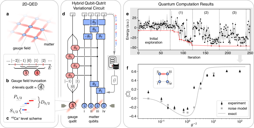
Figure 1: Simulating two-dimensional lattice QED with matter fields. a, The lattice of 2D-QED is comprised of vertices containing matter particles (blue) connected by links carrying the associated gauge field (red). The local gauge field at a particular link possesses an infinite, yet discrete spectrum that can be simulated using a truncated representation. b, The truncated gauge fields are naturally represented by $d$-level qudits. c, In our experiment these qudits (red) are encoded in different Zeeman levels of the S_1/2 ground state and D_5/2 excited state of trapped ${}^{40}\mathrm{Ca}^{+}$ ions. Matter particles, on the other hand, are faithfully represented by qubits (blue), marking their presence or absence. d, Our variational ansatz for simulating a single plaquette with open boundary conditions is thus a mixed-dimensional qubit-qudit quantum circuit, see Sec. III. Employing Gauss’ law to eliminate three of the four gauge fields, we truncate the remaining field to contain at most one energy quantum, hence our quantum register contains one qutrit (red) for the gauge field and four qubits (blue) representing the matter vertices of the plaquette. A fanning-out of the qudit circuit line is used to illustrate the coupling of the qudit entangling gates to certain subspaces, see also Appendix D1. Note that the all-to-all connectivity of the ion trap quantum processor enables a highly efficient circuit realization. During the variational optimization, a classical optimizer varies the gate angles $\theta_{j}$ in order to minimize the energy of the produced quantum state, as measured by the quantum computer. e, An exemplary optimization run for $g^{-2}=10^{2}$. The red line shows the current lowest energy found by the algorithm. Here, the first block of 71 evaluations sets up a grid in parameter space, while the subsequent block of 50 evaluations (1) optimizes the energy at $g^{-2}=10^{2}$. Each following block of 60 evaluations ((2), (3), … not all shown) is used to optimize for a different value of $g^{-2}$, while at the same time providing refinement for all other values of $g^{-2}$, see Appendix D2. One standard deviation of statistical uncertainty is given by the shaded region. Once an optimal set of parameters $\mathbf{\theta}^{*}$ is found, the properties of the so-created approximate (ground) state can be studied. f, The expectation value of the plaquette operator $\langle\hat{\square}\rangle$ as defined in the main text. The triangular data points are measured on the VQE optimized state, with error bars representing one standard deviation of statistical noise. The squares are obtained from a numerical simulation of an ideal VQE, with an experimentally motivated noise model applied to the final state, see Appendix H). The line is obtained from a classical calculation of the exact ground state, using exact diagonalization.

Quantum simulations of 2D-LGTs face the difficulty of finding an adequate representation for the gauge field operators $\hat{E}$. While the fermionic field can be straightforwardly transformed to qubits Jordan and Wigner (1928), whose states either represent the presence or absence of a particle (see Appendix C and Fig. B4c), the gauge field requires a truncation of its spectrum and a description containing at least three quantum states, representing positive, zero, and negative flux values. In principle, such a representation could be constructed from qubits. However, in practice, using qubits drastically increases the quantum register size and immediately results in complex many-body interactions Paulson et al. (2021), see Appendix E for details. For example, encoding $d$-level gauge fields requires at least $\lceil\mathrm{log}_{2}(d)\rceil$ qubits and even the application of local gauge field operators involves $\mathcal{O}(d^{2})$ two-qubit gates Sawaya et al. (2020). Gauss’ law requires that the creation or annihilation of particles occurs with the corresponding change in flux, which necessitates the application of gauge-field rising or lowering operators that are controlled by the state of the matter configuration, see Appendix Eq. (B1). Implementing such controlled gauge-field operations requires an even higher qubit gate count than the local gauge field operators. We circumvent this issue by representing each gauge field directly with a qudit system, containing exactly as many levels as required for the chosen truncation. As a consequence, local operations on the gauge fields remain local in the quantum computer, and the coupling between a matter site and a gauge field is realized as a two-body qubit-qudit interaction. We achieve an efficient implementation of these interactions through the use of explicit entanglement between the ion’s internal state and the common motional mode in the spirit of the seminal Cirac-Zoller gate Cirac and Zoller (1995). Conditional on the state of one ion (regardless of qudit dimension) a phonon is injected into the motional mode. If the phonon is present, a local operation is performed on the second ion, otherwise not. In the end, the phonon is deterministically removed from the motional mode and the internal states of the two ions are left entangled, see Appendix A for details. We realize both – qubits for matter fields and qudits for gauge fields – within the $4S_{1/2}$ ground state and the $3D_{5/2}$ excited state manifolds of trapped ${}^{40}\mathrm{Ca}^{+}$ ions Ringbauer et al. (2022), and thereby demonstrate quantum computations with tailored mixed-dimensional quantum systems. As shown in Fig. 1d and Appendix D2, we perform a variational ground-state search, using a suitable ansatz in the form of a quantum circuit with gates that are parameterized by a set $\mathbf{\theta}$ (see Sec. III below). A classical optimizer then varies the gate parameters to minimize the energy $\langle\hat{H}\rangle$ of the prepared states, which serves here as a cost function and is measured by the quantum computer. This optimization loop is repeated until the energy is minimized and one obtains a parameter set $\mathbf{\theta}^{*}$, such that the ansatz approximates the ground state of $\hat{H}$.

III Simulating gauge fields and matter

In our first experiment, we study 2D-QED on a lattice with open boundary conditions, crucially including both matter and gauge fields. In contrast to previous experiments (simulating LGTs in 1D or without matter) we observe the effects of virtual pair-creation, electromagnetic fields, and their interplay Paulson et al. (2021) by studying the ground state expectation value of the plaquette operator $\langle\hat{\square}\rangle=-\frac{1}{V}\langle\hat{H}_{B}\rangle$. Specifically, we consider the basic building block of the two-dimensional lattice, i.e. a single plaquette with open boundary conditions, consisting of four matter sites and four gauge fields, see inset in Fig. 1f. These gauge and matter degrees of freedom are constrained by Gauss’ law in Eq. (B4) at each vertex. These constraints can be encoded explicitly into an effective Hamiltonian, in which redundant gauge degrees of freedom are eliminated, see Appendix C. As a result, the resource requirements for our quantum computation are significantly reduced, while at the same time, the simulated states are guaranteed to be physical, i.e. obey Gauss’ law. The effective Hamiltonian per plaquette then involves only one gauge field. Employing the minimal gauge field truncation using three levels (i.e. $d=3$), our VQE ansatz is then given by a hybrid qudit-qubit approach with one qutrit representing the gauge degree of freedom, and four qubits representing electrons and positrons residing on the four vertices, see Fig. 1d.

This ansatz is based on the effective Hamiltonian given in Eq. (C7) and reflects the underlying physics of pair creation processes: the qubit states $\ket{\downarrow}/\ket{\uparrow}$ represent vacuum/electrons on even lattice sites and positrons/vacuum on odd lattice sites, as shown in Fig. B4 in the Appendix. The qutrit states $\{\ket{-1},\ket{0},\ket{+1}\}$ represent the electric field eigenstates of the gauge field. The circuit is initialized in the qudit-qubit state $\ket{\downarrow\uparrow\downarrow\uparrow,0}$, representing the bare vacuum $|vvvv,0\rangle$, where no particles (first four entries) or gauge field excitations (last entry) are present. As shown in Fig. 1d, the two-qubit gates on the matter qubits (blue) at the beginning of the circuit populate the plaquette with electrons and positrons. When the two lattice sites directly next to the remaining gauge field are populated (see inset of Fig. 1f), Gauss’ law requires the excitation of the gauge field to change accordingly, which is achieved by the qubit-qutrit controlled-rotation gates (red). In the final part of the circuit, four two-qubit gates (blue) adjust the matter state. This last step can be done without modifying the state of the qutrit, since the matter fields also have gauge-field-independent free dynamics. The described Hamiltonian-based VQE circuit design is extendable to larger lattices as explained in Ref. Paulson et al. (2021).

Figure 1e shows a typical experimental run of the variational circuit. The resulting measured plaquette expectation values as a function of the parameter $g^{-2}$ are shown in Fig. 1f for $\Omega=5$ and $m=0.1$. The experimental data approximate the ideal result well and agree with our theoretical predictions using a simple error model, as explained in Appendix H. In the large coupling regime ($g^{-2}\ll 1$) the electric field energy term $\hat{H}_{E}$ dominates the Hamiltonian of Eq. (1), favoring the ground state $|vvvv,0\rangle$ with $\langle\hat{\square}\rangle=0$. In the weak coupling regime, on the other hand, the magnetic field energy term $\hat{H}_{B}$ dominates the Hamiltonian, favoring a positive vacuum plaquette expectation value ($\langle\hat{\square}\rangle=\frac{1}{\sqrt{2}}\approx 0.707$ for the chosen truncation). In the intermediate regime where $g^{-2}\approx 1$, we encounter a competition between the two field-energy terms and $\hat{H}_{k}$. The presence of the kinetic term $\hat{H}_{k}$ makes it energetically favorable to create pairs, which in turn produce a background magnetic flux that opposes the flux present in the ground state preferred by the term $\hat{H}_{B}$. On its own, the term $\hat{H}_{k}$ leads to a ground state with a negative plaquette expectation value ($\langle\hat{\square}\rangle=-0.642$ in the considered case). The presence of dynamical matter, therefore, results in a reduction of the plaquette expectation value in the ground state, as shown in Fig. 1f. Notably, even with our small system size we already clearly observe the dip in the plaquette expectation value that originates from pair creation processes in the ground state, see Ref. Paulson et al. (2021) for details.

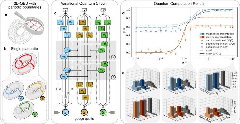
Figure 2: Refining the gauge field discretization a, We consider pure gauge QED in two spatial dimensions with periodic boundary conditions, i.e. on a lattice on the surface of a torus. As before, the gauge field resides on the links of the lattice, while here the vertices remain empty. b, We consider the smallest instance of such a torus, containing four empty sites and eight gauge field links. The ground state of this particular system can be described via three separate circulation-paths of the gauge field, called rotators as discussed in Appendix C2. Each rotator fulfills an eigenvalue equation equivalent to a single link gauge field and can thus be subject to the same truncation rules as discussed in the main text by employing a $d$-level qudit. Here, we demonstrate the difference between a realization employing qutrits and ququints. c, The variational circuit in the electric representation (see main text) for the qutrit (solid lines) and the ququint (all, except shaded box marked with qutrit symbol) truncation. The explicit form of the gates employed is given in Appendix D1. d, Experimentally measured ground-state expectation values of the plaquette operator $\hat{\square}$ using qutrits (VQE optimized) compared to ququints (direct preparation with one VQE-optimized point in the highly-entangled regime of the electric representation at $g^{-2}{=}10^{2}$). The error bars indicate one sigma statistical uncertainty. The black line represents numerical results obtained for $d=21$, using the electric (magnetic) representation for small (large) values of $g^{-2}$. e, The duality between the electric (all orange bars) and magnetic (all blue bars) representations is clearly seen in the experimentally measured populations of the eigenvectors of the yellow rotator from panel b for the qutrit VQE experiment and ququint experiment. The grey bars are results obtained via exact diagonalization. In the regime dominated by the electric Hamiltonian (small $g^{-2}$) a qutrit (light orange) representation is enough to approximate the correct ground state, while for larger $g^{-2}$ truncation errors become more relevant and a ququint representation (dark orange) becomes advantageous. A complementary argument applies to the magnetic qutrit (light blue) and ququint (dark blue) representation.

IV Towards refining the gauge field discretization

While our results in Fig. 1f show that the relevant physics is already captured even for the minimal truncation of $d=3$, we now turn our attention to controlling the number of gauge field levels. More specifically, we demonstrate how our qudit platform allows us to seamlessly improve the gauge field discretization from qutrits ($d=3$) to ququints ($d=5$). As a concrete example, we study the dependence of the plaquette expectation value on the bare coupling at different discretizations, as a first important step towards quantum computations of the running of the coupling. To this end, we consider QED on a 2D lattice with periodic boundary conditions, which takes the form of a torus, see Fig. 2a.

For our proof-of-concept demonstration, we consider a pure gauge theory $\hat{H}=g^{2}\hat{H}_{E}+(1/g^{2})\hat{H}_{B}$, see Eq. (B2). Fig. 2b shows the minimal system consisting of four vertices and eight gauge fields (one per link). Using Gauss’ law we reduce the number of independent gauge fields to five, and it can be shown that three of these are sufficient to describe ground state properties Haase et al. (2021). Instead of describing the gauge degrees of freedom in terms of the fields associated with the individual links of the lattice as before, we switch to a more convenient description in terms of operators called “rotators”. As explained in Ref. Haase et al. (2021), each of the three rotators in our simulation can be visualized as loops around a different plaquette, see Fig. 2b.

So far, we truncated the gauge field directly in the electric field eigenbasis, i.e. in our first experiment we included eigenstates $|E\rangle$ of the electric field operator $\hat{E}$ with $\hat{E}|E\rangle=E|E\rangle$ and $E=0,\pm 1$. However, to determine the plaquette expectation value resource-efficiently across all values of the coupling, we now employ a more suitable truncation scheme that we introduced in Ref. Haase et al. (2021). Our method is based on a Fourier transformation: for large couplings (where $g^{-2}\ll 1$), the Hamiltonian is dominated by the electric field contribution $\hat{H}_{E}$, and a gauge field truncation in the electric (E-) field basis is suitable, which we refer to as the electric representation. For small couplings (where $g^{-2}\gg 1$), the magnetic field term dominates, and accordingly, a magnetic (B-) field basis (using B-field eigenstates) is more efficient. The VQE circuits for the E- and B- representations are shown in the Appendix and in Fig. 2c respectively. As explained in Appendix F, their construction is inspired by the form of the Hamiltonian.

Figure 2d shows the resulting ground-state plaquette expectation values versus $g^{-2}$, along with our theoretical predictions that include a simple noise model, as described in Appendix H. For the ququints, we perform the VQE for one point in the highly-entangled regime of the electric representation at a bare coupling of $g^{-2}{=}10^{2}$, and a direct preparation (i.e. perform the circuit in Fig. 2c for optimal parameters $\theta$) for the whole range of couplings. For qutrits, we performed the full VQE as in Fig. 1. Note that we show the results for both representations across all values of the coupling $g^{-2}$, even though the validity of the electric (magnetic) representation is restricted to the large (small) coupling regime, where $g^{-2}\ll 1$ ($g^{-2}\gg 1$). The gap between the curves in the intermediate region $g^{-2}\approx 1$, where the electric and magnetic representations perform equally, stems from the truncation of the gauge fields, see Ref. Haase et al. (2021). As the truncation is increased, the two curves rapidly approach each other and eventually agree for some intermediate value of $g^{-2}$, as indicated by the experimental data and confirmed by a numerical simulation at $d=21$, see Fig. 2d. The value of $g^{-2}$ where the curves are closest indicates the point at which the representation should be switched.

This effect can also be observed in Fig. 2e, where we depict the measured populations of the gauge fields in the ground state. In the large coupling regime (where $g^{-2}\ll 1$), the distribution of electric field states is narrow, which allows for an efficient truncation in the E-basis. By contrast, this distribution becomes very broad in the small coupling regime, where it tends to an equally weighted superposition of infinitely many E-field levels in the limit $g^{-2}\gg 1$. As a result, the accurate approximation of the ground state in the E-basis implies exploding resource costs without a basis change Haase et al. (2021). The behavior of the B-representation is complementary. The aforementioned closing of the gap between the plaquette expectation values in the E-representation (red) and the B-representation (blue) in Fig. 2d thus corresponds to a better representation of the ground state in Fig. 2e. The closing gap for intermediate values of $g^{-2}$ provides an indication of how well LGT quantum computations with finite $d$ approximate the untruncated results Haase et al. (2021).

Similarly, the so-called “freezing” of the truncated plaquette expectation value (the dashed blue lines for $d=3,5$ in Fig. 2d flatten out earlier than the solid black line for $d=21$) in the weak coupling regime $g^{-2}\gg 1$ serves as an indicator for how well the ground state is approximated. Freezing occurs in both classical and quantum computations if the number of levels $d$ is insufficient to capture the fine features of the theory. A detailed explanation and analysis are provided in Ref. Haase et al. (2021), showing fast convergence of the plaquette expectation value to the true value already for moderate values of $d\leq 10$. Hence, the number of available internal states in typical atomic systems is sufficient for reaching a good representation of the ground state. Notably, our experimental setup allows for improving the gauge field discretization from $d=3$ to $d=5$ with only minor modifications, involving the same number of ions and the same number of entangling gates, see Appendix.

V Outlook

Qudits provide a hardware-efficient approach to quantum-simulating gauge theories. Using a universal trapped-ion qudit quantum computer with all-to-all connectivity enables us to simulate arbitrary geometries, and thus perform quantum simulations of 2D-LGTs. In particular, we are able to simulate a basic building block of 2D-QED with both dynamical matter and gauge fields. These complex computations are rendered possible by high-fidelity qudit control, combined with VQE circuits that are much shallower than comparable qubit-based implementations of gauge theory calculations. While we exploit native qudit circuits to study equilibrium properties, the techniques we developed are directly adaptable to digital quantum simulations of real-time dynamics Nguyen et al. (2022). This offers an exciting perspective for quantum simulations of LGT dynamics in regimes that are classically intractable due to sign problems Robaina et al. (2021); Banuls et al. (2019).

The ultimate goal is to simulate nature in three spatial dimensions. Importantly, there is a dramatic change in the simulation requirements from 1D to 2D, while there is little change going from 2D to the full 3D model Kan et al. (2021); Zohar (2021). In particular, while the high-dimensional gauge fields can be integrated out in 1D models, they are dynamical degrees of freedom in 2D and 3D and must be simulated explicitly. Our results on QED simulations beyond 1D thus represent a major step towards simulating 3D LGTs. In particular, our protocol based on eliminating redundant gauge degrees of freedom employed here can be directly extended to 3D (in the case of QED shown in Ref. Kan et al. (2021)). Our qudit techniques can be applied to virtually all other quantum computing architectures and hardware platforms. For all of them, the remaining major task is scaling up the system sizes, which makes an efficient gauge field representation even more important. Beyond just programmable local dimensions, qudit-based systems enjoy larger freedom for designing interactions to match the target problem for a highly efficient implementation. Our demonstration of a qudit-based quantum simulation of high-energy physics phenomena paves the way to a new generation of qudit-based applications in all areas of quantum technology.

Appendix A Realizing controlled rotations in qudits

We encode each qudit in Zeeman states of trapped ${}^{40}\mathrm{Ca}^{+}$ ions and manipulate their quantum state by sequences of laser pulses. Doppler cooling and state detection is performed by driving the short-lived $S_{\nicefrac{{1}}{{2}}}\longleftrightarrow P_{\nicefrac{{1}}{{2}}}$ transition, monitoring the fluorescence of the individual ions on a CCD camera; a simplified level scheme of the relevant states is shown in Fig. A1. Quantum gate operations are implemented by selectively addressing single – or arbitrary pairs of – ions via a high numerical aperture objective, coupling the $D_{\nicefrac{{5}}{{2}}}$ manifold with the $S_{\nicefrac{{1}}{{2}}}$ ground states Kim et al. (2008). Due to the geometry of our ion trap, the beam is aligned at an angle of $22.5^{\circ}$ with respect to the trap axis, leading to a Lamb-Dicke factor of $\eta=0.041$ for an axial trap frequency of $\omega_{z}=0.77~{}\mathrm{MHz}$. We measure a heating rate of $2.7(2)$ phonons per second and a motional coherence time $\tau$ of $27.4(4)~{}\mathrm{ms}$.

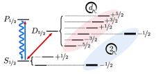
Figure A1: Simplified level scheme of ${}^{40}\mathrm{Ca}^{+}$. Doppler cooling and state detection is performed on the short-lived $S_{\nicefrac{{1}}{{2}}}\leftrightarrow P_{\nicefrac{{1}}{{2}}}$ transition with a life time of $\approx 9~{}\mathrm{ns}$. Qubits are encoded in the Zeeman states $\ket{0}=S_{m=-\nicefrac{{1}}{{2}}}$ and $\ket{1}=D_{m=-\nicefrac{{1}}{{2}}}$, while qudits are encoded only in the $D_{\nicefrac{{5}}{{2}}}$ manifold. Any excitation of a $D_{\nicefrac{{5}}{{2}}}$ state decays in $T_{1}\approx 1.1~{}\mathrm{s}$ to the $S_{\nicefrac{{1}}{{2}}}$ ground states; this transition is addressed by a narrow-band laser with a coherence time of $T_{2}=92(9)~{}\mathrm{ms}$.

Qudits with dimension $d=2$ (i.e. qubits) are encoded, such that $\ket{0}=S_{\nicefrac{{1}}{{2}}}(m=-1/2)$ and $\ket{1}=D_{\nicefrac{{5}}{{2}}}(m=-1/2)$ as shown in Fig. A1. For $d>2$ only the $D_{\nicefrac{{5}}{{2}}}$ manifold of ${}^{40}\mathrm{Ca}^{+}$ is used for encoding the qudit, while the $S_{1/2}$ ground states act as auxilliary levels $\ket{g}$, which are only populated during gate operations and readout.

Mixed-dimensional qudit-qudit interactions are engineered by controllably coupling qudits to a single phonon mode, effectively, using an Anti-Jaynes-Cummings Hamiltonian described by

$$H_{j}=i\eta\Omega_{j}\left(\hat{a}^{\dagger}\sigma^{+\ket{k}}_{j}+\hat{a}\sigma^{-\ket{k}}_{j}\right),$$

on the $j$-th ion with Rabi frequency $\Omega_{j}$. Here, $\hat{a}^{\dagger}\sigma^{+}_{j}$ excites the qudit from the (auxilliary) ground state $\ket{g}$ from the $S_{\nicefrac{{1}}{{2}}}$ manifold to a state $\ket{k}$ the $D_{\nicefrac{{5}}{{2}}}$ manifold, while injecting a phonon into the motional mode. In our setup, we realize this interaction by driving controlled laser pulses $B(\theta,\phi)$ tuned to the first (blue) sideband (BSB) of the axial center-of-mass (COM) motional mode. This mode is favorable due to the homogenous coupling for all ions in the string and the reduced calibration effort, as all laser pulses have close to identical parameters for all qudits.

Envisioned to realize the Cirac-Zoller controlled-NOT (CNOT) quantum gate in trapped ions Cirac and Zoller (1995), this approach is well suited to implement mixed-dimensional controlled rotations (C-ROTs) in qudits as shown in Fig. A2. Here, we consider a two-level subspace of a qudit, described by the states $\ket{0}$ and $\ket{1}$, which can be coupled to the motional mode $\ket{n}$ via an auxiliary ground state $\ket{\mathrm{aux}.}$. We bring the control state – here $\ket{1}$ – of the control qudit to $\ket{\mathrm{aux.}}$ via a resonant interaction, before bringing it back to the original state and exciting the motion by a $\pi$-pulse $B(\pi,0)$ on the BSB, entangling the system with the COM mode. It is evident that this operation has no effect if the control qudit is initially not in the state $\ket{1}$. On the target qudit, we apply a sequence of three sideband pulses, namely

$$B(\pi,0)^{\ket{\mathrm{aux.}}\to\ket{1}}B(\theta,\phi)^{\ket{\mathrm{aux.}}\leftrightarrow\ket{0}}B(-\pi,0)^{\ket{1}\to\ket{\mathrm{aux.}}},$$

where the superscripts indicate the respective coupling between the state $\ket{\mathrm{aux.}}$ and the states $\ket{0},\ket{1}$. Crucially, these operations affect the target qudit only if the phonon mode is excited. In the final step, the initial operations on the control qudit are applied in reversed order, disentangling the control qudit from the COM mode and restoring their initial states.

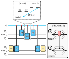
Figure A2: Qudit circuit for implementing a mixed-dimensional controlled rotation (C-ROT) gate. For each 5-dimensional qudit (right), we consider a two-level subspace (left), containing the states $\ket{0}$ and $\ket{1}$, coupled to an auxiliary ground state $\ket{\mathrm{aux.}}$. After an initial transfer of the control state $\ket{1}_{c}$ to the auxiliary level (yellow), the motional mode $\ket{n}$ is excited by a blue sideband (BSB) pulse $B(\theta,\phi)$, entangling the ion qudits with the phonon mode (blue). Conditional on the phonon being present in the motional mode, further BSB pulses act locally on the target qudit. At the end of the sequence, the qudits are again disentangled from the motion. In the inset on the right, we introduce a symbol for the C-ROT operation $CROT(\theta,\phi)$, which allows us to draw controlled qudit operations in quantum circuits in a similar manner to qubit gates, see e.g. Fig. 1d.

We extend the well-established circuit representation of quantum gates in qubits by introducing a way to draw interactions in qudits in a similar manner. As shown in the panel in Fig. A2, we expand the line representing each qudit into $d$ individual rails, allowing us to draw gates acting on subspaces of the qudit unambiguously, and contract the rails back to a single line after the subspace gate. In the case of C-ROTs, the control state is indicated in the usual fashion.

As the Rabi frequency on the BSB is proportional to the Lamb-Dicke factor $\eta$, driving the blue sideband requires substantially more laser power than carrier transitions. Each $B(\theta,\phi)^{\ket{g}\leftrightarrow\ket{k}}$ will thus introduce unwanted AC Stark shifts $\Delta_{\mathrm{AC}}$ on the order of a few $\mathrm{kHz}$ Ringbauer et al. (2022), which must be carefully taken into account for achieving high-fidelity C-ROT gates. We compensate the $\Delta_{\mathrm{AC}}$ using a two-fold approach: (1) shifts on the actively driven BSB transition are compensated by an off-resonant second-beam technique Häffner et al. (2003); Meth et al. (2022), while (2) additional shifts on spectator carrier transitions $\ket{l\neq k}$ are measured and compensated in software by frame updates on subsequent operations. An example of shifted spectator states is shown in Fig. A3 for $B(\theta,\phi)$ on the blue sideband of the transition $S_{-1/2}\leftrightarrow D_{-1/2}$ with a Rabi frequency $\tilde{\Omega}=2\pi\cdot 4~{}\mathrm{kHz}$. For each state $\Delta_{\mathrm{AC}}$ is obtained by a Ramsey measurement.

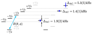
Figure A3: AC stark shifts on spectator levels for an excitation of the blue sideband of the $S_{-1/2}\leftrightarrow D_{-1/2}$ transition. While the AC Stark shift on this transition is directly compensated by a second, off-resonant laser beam, the spectator levels $D_{-5/2}$, $D_{+1/2}$ and $D_{+3/2}$ remain shifted by a few $\mathrm{kHz}$ with respect to the $S_{-1/2}$ ground state. The individual blue dots correspond to different runs over the course of several days and the uncertainty represents one standard deviation of the fit uncertainty. These spectator shifts are compensated in software by storing a phase register for each qudit state and phase-shifting the subsequent operations on the affected qudit transitions by an appropriate amount.

Appendix B 2D-QED Hamiltonian

The models we simulate are instances of lattice QED and are defined on a two-dimensional discretization of space. Matter (electrons and positrons) and gauge bosons (photons) are defined on the sites and on the links of this lattice respectively, as shown in Fig. 1a.

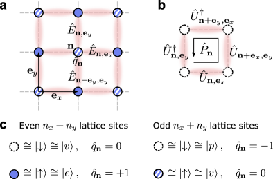
Figure B4: Elements of two-dimensional lattice QED. a, 2D lattice for the Kogut-Susskind Hamiltonian formulation. On each site $\mathbf{n}=(n_{x},n_{y})$ resides a fermionic field operator $\hat{\phi}_{\mathbf{n}}$ that represents the presence or absence of particles. Each site can either be in the vacuum state or occupied by an electron (positron) for even (odd) sites. Electrons (positrons) are shown as filled circles with solid (striped) color, see panel c. The gauge bosons are described by operators on the links of the lattice. b, The operator $\hat{P}_{\mathbf{n}}$ is defined around a counterclockwise path around the plaquette with origin in $\mathbf{n}$. For every link, $\hat{P}_{\mathbf{n}}$ acquires a factor $\hat{U}$ if the path goes towards the positive directions $\mathbf{e}_{\mu}$, with $\mu\in\{x,y\}$, and a factor $\hat{U}^{\dagger}$ otherwise. c, Mapping between fermionic states, qubit states (obtained via a Jordan-Wigner transformation), and physical states, including associated charges.

Here, matter is described by fermionic field operators $\hat{\phi}_{\mathbf{n}}$ with spatial label $\mathbf{n}=(n_{x},n_{y})$. We employ the staggered formulation Kogut and Susskind (1975), in which lattice sites can either be in the vacuum state or host electrons (positrons) residing on even (odd) lattice sites, carrying a $+1$ ($-1$) charge, as depicted in Fig. B4. The charge in terms of the fermionic field is given by $\hat{q}_{\mathbf{n}}=\hat{\phi}_{\mathbf{n}}^{\dagger}\hat{\phi}_{\mathbf{n}}-\frac{1-(-1)^{n_{x}+n_{y}}}{2}$.

The gauge field residing on the links between each pair of sites is described by an electric field operator $\hat{E}_{\mathbf{n},\mathbf{e}_{\mu}}$ ($\mu\in\{x,y\}$) that possesses an infinite but discrete spectrum $\hat{E}_{\mathbf{n},\mathbf{e}_{\mu}}\ket{E_{\mathbf{n},\mathbf{e}_{\mu}}}=E_{\mathbf{n},\mathbf{e}_{\mu}}\ket{E_{\mathbf{n},\mathbf{e}_{\mu}}}$, where $E_{\mathbf{n},\mathbf{e}_{\mu}}=0,\,\pm 1,\,\pm 2,\dots$. The link operator $\hat{U}_{\mathbf{n},\mathbf{e}_{\mu}}$ acts as a lowering operator for the electric field:

$$\hat{U}_{\mathbf{n},\mathbf{e}_{\mu}}\ket{E_{\mathbf{n},\mathbf{e}_{\mu}}}=\ket{E_{\mathbf{n},\mathbf{e}_{\mu}}-1}.$$ (B1)

The total Hamiltonian is then given by a sum of four parts as shown in Eq. (1). Note that compared to the convention used in Haase et al. (2021); Paulson et al. (2021) we have opted to redefine the four Hamiltonians such that they are independent of the mass and coupling constant. More explicitly, by employing the Kogut-Susskind formulation in natural units $\hbar=c=1$, and with lattice spacing $a=1$, these terms read

$$\hat{H}_{E} =\frac{1}{2}\sum_{\mathbf{n}}\left(\hat{E}_{\mathbf{n},\mathbf{e}_{x}}^{2}+\hat{E}_{\mathbf{n},\mathbf{e}_{y}}^{2}\right),$$ (B2a)

$$\hat{H}_{B} =-\frac{1}{2}\sum_{\mathbf{n}}\left(\hat{P}_{\mathbf{n}}+\hat{P}_{\mathbf{n}}^{\dagger}\right),$$ (B2b)

$$\hat{H}_{m} =\sum_{\mathbf{n}}(-1)^{n_{x}+n_{y}}\hat{\phi}_{\mathbf{n}}^{\dagger}\hat{\phi}_{\mathbf{n}},$$ (B2c)

$$\hat{H}_{k} =\sum_{\mathbf{n}}\sum_{\mu=x,y}\left(\hat{\phi}_{\mathbf{n}}\hat{U}_{\mathbf{n},\mathbf{e}_{\mu}}^{\dagger}\hat{\phi}_{\mathbf{n}+\mathbf{e}_{\mu}}^{\dagger}+\mathrm{H.c.}\right).$$ (B2d)

$\hat{H}_{E}$ and $\hat{H}_{B}$ represent the free electric and magnetic field, while $\hat{H}_{m}$ and $\hat{H}_{k}$ describe the free matter field and its interaction with the gauge field. The operator $\hat{P}_{\mathbf{n}}$ is defined on a counterclockwise closed loop around the plaquette with origin $\mathbf{n}$ (see Fig. B4b) as

$$\hat{P}_{\mathbf{n}}=\hat{U}_{\mathbf{n},\mathbf{e}_{x}}\hat{U}_{\mathbf{n}+\mathbf{e}_{x},\mathbf{e}_{y}}\hat{U}_{\mathbf{n}+\mathbf{e}_{y},\mathbf{e}_{x}}^{\dagger}\hat{U}_{\mathbf{n},\mathbf{e}_{y}}^{\dagger}.$$ (B3)

Noting that the link operator $\hat{U}_{\mathbf{n},\mathbf{e}_{\mu}}$ is expressed in terms of the gauge fields’ vector potential $\hat{A}_{\mathbf{n},\mathbf{e}_{\mu}}$, i.e. $\hat{U}_{\mathbf{n},\mathbf{e}_{\mu}}\sim\mathrm{exp}\{ig\hat{A}_{\mathbf{n},\mathbf{e}_{\mu}}\}$, one observes that the exponent of $\hat{P}_{\mathbf{n}}$ forms a discrete lattice curl of the vector potential. The plaquette operator $\hat{\square}=\frac{1}{2V}\sum_{\mathbf{n}}\left(\hat{P}_{\mathbf{n}}+\hat{P}_{\mathbf{n}}^{\dagger}\right)$, where $V$ is the number of plaquettes, is therefore proportional to the magnetic field energy and a true multi-dimensional quantity which has no analog in 1D-QED. In quantum field theories the spontaneous creation of particle/antiparticle pairs in vacuum means that, when measuring the strength of a charge, the result can depend on the distance and energy scale at which it is probed. Since the coupling is proportional to the charge Hamer et al. (1997), this means that the physical coupling, which is an important parameter in phenomenological HEP models, also depends on the energy scale. This phenomenon is known as the running of the coupling. The dependence of the ground-state plaquette expectation value $\langle\hat{\square}\rangle$ on $g^{-2}$, where $g$ is the bare coupling, can be related to the running of the coupling and it is discussed more in detail in Clemente et al. (2022).

Importantly, not all quantum states in the considered Hilbert space are physical. The gauge field and charge configurations of physical states $|\Psi_{\text{phys}}\rangle$ have to fulfill Gauss’ law at every site. Here, the familiar law from classical electrodynamics $\nabla\mathbf{E}(\mathbf{r})-\rho(\mathbf{r})=0$, where $\rho(\mathbf{r})$ is the charge density at point $\mathbf{r}$, takes the form

$$\hat{G}_{\mathbf{n}}|\Psi_{\text{phys}}\rangle=0,$$ (B4)

where the Gauss’ operator is defined as

$$\hat{G}_{\mathbf{n}}=\sum_{\mu}(\hat{E}_{\mathbf{n},\mathbf{e}_{\mu}}-\hat{E}_{\mathbf{n}-\mathbf{e}_{\mu},\mathbf{e}_{\mu}})-\hat{q}_{\mathbf{n}}.$$ (B5)

In general, Gauss’ law requires physical states to be eigenvectors of the Gauss operator; we have made the choice in Eq. (B4) to consider the eigenvalues to be zero, which describes a model with no external charges. The total charge $\sum_{\mathbf{n}}\hat{q}_{\mathbf{n}}$ can be shown to also be a symmetry of the Hamiltonian. In this work, we choose to study states that have zero total charge.

Appendix C Encoded Hamiltonian

In the following, we provide the Hamiltonians studied via the VQE circuits given in Fig. 1d and Fig. 2c.

C1 2D-QED with matter

Let us consider a single plaquette with open boundary conditions with origin in $\mathbf{n}=(0,0)$, as shown in the inset of Fig. 1f. As was discussed in Paulson et al. (2021), Gauss’ law given in Eq. (B4) can be used to eliminate three gauge fields, resulting in an effective Hamiltonian that contains four fermionic fields and one gauge field, which we choose to be the one between sites ii and iii. We encode the fermions i$,\dots,$ iv (conventionally ordered clockwise around the plaquette) into a chain of qubits indexed by $1,\dots,4$ respectively by applying the following Jordan-Wigner transformation

$$\hat{\phi}_{i}=\prod_{j<i}(-\hat{\sigma}_{j}^{z})\hat{\sigma}_{i}^{-},\quad\hat{\phi}_{i}^{\dagger}=\prod_{j<i}(-\hat{\sigma}_{j}^{z})\hat{\sigma}_{i}^{+}.$$ (C6)

In particular, the charge associated to each site is now given by $\hat{q}_{i}=\frac{\hat{\sigma}_{i}^{z}+(-1)^{i+1}}{2}$. A table summarizing how the spin states are related to the fermionic states is given in Fig. B4c.

The Hamiltonian given by the Jordan-Wigner transformation reads

$$\begin{split}\hat{H}_{E}&=\frac{1}{4}(8\hat{E}+2\hat{E}\left(-\hat{\sigma}^{z}_{1}-2\hat{\sigma}^{z}_{2}+3\hat{\sigma}^{z}_{3}+2\right)\\ &\qquad\quad-\hat{\sigma}^{z}_{2}+\hat{\sigma}^{z}_{3}+\hat{\sigma}^{z}_{1}\hat{\sigma}^{z}_{2}+3),\end{split}$$ (C7a)

$$\hat{H}_{B} =-\frac{1}{2}\left(\hat{U}+\hat{U}^{\dagger}\right),$$ (C7b)

$$\hat{H}_{m} =\frac{1}{2}\left(\hat{\sigma}^{z}_{1}-\hat{\sigma}^{z}_{2}+\hat{\sigma}^{z}_{3}-\hat{\sigma}^{z}_{4}\right),$$ (C7c)

$$\hat{H}_{k} =-\hat{\sigma}^{+}_{1}\hat{\sigma}^{-}_{4}+\hat{\sigma}^{+}_{1}\hat{\sigma}^{-}_{2}+\hat{\sigma}^{+}_{4}\hat{\sigma}^{-}_{3}+\hat{\sigma}^{+}_{2}\hat{U}\hat{\sigma}^{-}_{3}+\text{H.c.},$$ (C7d)

where we have simplified terms in the kinetic Hamiltonian, by using the fact that we consider only states with zero total charge (and therefore zero total magnetization for the qubits), as discussed below Eq. (B4).

The gauge degree of freedom is encoded in a qutrit, and following Ref. Paulson et al. (2021), we truncate the gauge field operators as

$$\hat{E}=\begin{pmatrix}1&0&0\\ 0&0&0\\ 0&0&-1\end{pmatrix},\qquad\hat{U}=\begin{pmatrix}0&0&0\\ 1&0&0\\ 0&1&0\end{pmatrix}.$$ (C8)

C2 Pure gauge 2D-QED

The second simulated model is a pure gauge theory with periodic boundary conditions as shown in Fig. 2a. We consider here the minimal instance consisting of four vertices, as depicted in Fig. 2b. As discussed in Ref. Haase et al. (2021), Gauss’ law can be used to reduce the system to three independent degrees of freedom; these are described by three operators $\hat{P}_{i}$ ($i=1,2,3$) which are defined in Eq. (B3), and are each associated to the magnetic energy of a plaquette depicted in the lower part of Fig. 2b. For each plaquette we define the corresponding rotator operator as the circulation of the gauge field going counterclockwise. It can be shown that the rotators have integer spectrum

$$\hat{R}_{i}\ket{r_{i}}=\ket{r_{i}},r_{i}\in\mathbb{Z},$$ (C9)

and that the operators $\hat{P}_{i}$ act as lowering operators on these states, i.e. $\hat{P}_{i}\ket{r_{i}}=\ket{r_{i}-1}$.

In order to study this model on a quantum computer, the infinite-dimensional Hilbert spaces of the rotators need to be truncated with a strategy that allows one to systematically increase the truncation size and approach the continuum limit, as discussed in detail in Ref. Haase et al. (2021). We summarize here the essential points of the derivation. As a first step the gauge group $\operatorname{U(1)}$ is substituted by the discrete group $\mathbb{Z}_{2L+1}$, and the Hilbert space is then truncated for each rotator to the $2l+1$ eigenstates $\ket{-l},\dots,\ket{l}$, for some $l\leq L$. The action of the truncated $\hat{P}_{i}$ operator is then given by

$$\hat{P}_{i}\ket{r_{i}}=\begin{cases}\ket{r_{i}-1},\text{if }r_{j}>-l\\ \delta_{lL}\ket{l},\text{if }r_{j}=-l.\end{cases}$$ (C10)

The Hamiltonian in terms of the rotators reads

$$\hat{H}^{\text{(e)}} =g^{2}\hat{H}^{\text{(e)}}_{E}+\frac{1}{g^{2}}\hat{H}^{\text{(e)}}_{B},$$ (C11a)

$$\hat{H}^{\text{(e)}}_{E} =2\left[\hat{R}_{1}^{2}+\hat{R}_{2}^{2}+\hat{R}_{3}^{2}-\hat{R}_{2}\left(\hat{R}_{1}+\hat{R}_{3}\right)\right],$$ (C11b)

$$\hat{H}^{\text{(e)}}_{B} =-\frac{1}{2}\left(\hat{P}_{1}+\hat{P}_{2}+\hat{P}_{3}+\hat{P}_{1}\hat{P}_{2}\hat{P}_{3}+\text{H.c.}\right),$$ (C11c)

where we have used the superscript (e) to indicate that we are using here the so-called electric representation, in which the electric Hamiltonian $\hat{H}^{\text{(e)}}_{E}$ is diagonal. The parameter $g$ is the bare coupling and is proportional to the bare electric charge Hamer et al. (1997).

In the regime where $g\ll 1$, it is more convenient to apply a discrete Fourier transform to the Hamiltonian, which leads to a magnetic representation, where $\hat{H}^{\text{(b)}}_{B}$ is diagonal. For the calculations, let us define the following coefficients, defined in terms of the polygamma functions $\psi_{\nu}(x)$

$$f_{\nu}^{s} =\frac{(-1)^{\nu+1}}{2\pi}\left[\psi_{0}\!\left(\frac{2+L1+\nu}{2(2L+1)}\right)-\psi_{0}\!\left(\frac{\nu}{2(2L+1)}\right)\right],$$ (C12a)

$$f_{\nu}^{c} =\frac{(-1)^{\nu}}{4\pi^{2}}\left[\psi_{1}\!\left(\frac{\nu}{2(2L+1)}\right)-\psi_{1}\!\left(\frac{2L+1+\nu}{2(2L+1)}\right)\right],$$ (C12b)

and introduce the notation $\ket{\bm{r}}=\ket{r_{1}}\ket{r_{2}}\ket{r_{3}}$. The Hamiltonian in the magnetic representation is then given by

$$\hat{H}^{\text{(b)}} =g^{2}\hat{H}^{\text{(b)}}_{E}+\frac{1}{g^{2}}\hat{H}^{\text{(b)}}_{B},$$ (C13a)

$$\begin{split}\hat{H}^{\text{(b)}}_{E}&=\sum_{\nu=1}^{2L}\bigg{[}f_{\nu}^{c}\left(\hat{P}_{1}^{\nu}+\hat{P}_{2}^{\nu}+\hat{P}_{3}^{\nu}\right)\\ &\quad+\frac{f_{\nu}}{2}\left(\hat{P}_{2}^{\nu}-\left(\hat{P}_{2}^{\dagger}\right)^{\nu}\right)\sum_{\mu=1}^{2L}f_{\mu}^{s}\left(\hat{P}_{1}^{\mu}+\hat{P}_{3}^{\mu}\right)\bigg{]}+\text{H.c.},\end{split}$$ (C13b)

$$\begin{split}\hat{H}^{\text{(b)}}_{B}&=-\sum_{\bm{r}=-\bm{L}}^{\bm{L}}\Bigg{[}\cos\!\left(\frac{2\pi r_{1}}{2L+1}\right)+\cos\!\left(\frac{2\pi r_{2}}{2L+1}\right)\\ &\qquad+\cos\!\left(\frac{2\pi r_{3}}{2L+1}\right)+\cos\!\left(\frac{2\pi(r_{1}+r_{2}+r_{3})}{2L+1}\right)\Bigg{]}\outerproduct{\bm{r}}{\bm{r}}.\end{split}$$ (C13c)

For our quantum calculations shown in Fig. 2 we choose $(L,l)=(2,1)$ for the qutrit experiment, and $(L,l)=(3,2)$ for the ququint experiment. Throughout the paper we use $L=l+1$.

Appendix D A Variational Quantum Eigensolver for Qudits

D1 Variational circuit

As explained in the main text, the variational circuit shown in Fig. 1d is designed based on the form of the target Hamiltonian given in Eqs. (C7). Since all the coefficients of the Hamiltonian are real, it is convenient to use gates in the variational circuit that rotate between states with real coefficients only. This approach also allows us to formulate a circuit that is more efficient in the number of variational parameters. In particular, the square blue gates between qubits are the magnetization-conserving gates studied in Ref. Gard et al. (2020), defined as

$$A(\theta,\phi)=\left(\begin{matrix}1&0&0&0\\ 0&\cos\theta&e^{i\phi}\sin\theta&0\\ 0&e^{-i\phi}\sin\theta&-\cos\theta&0\\ 0&0&0&1\\ \end{matrix}\right).$$ (D14)

We choose $\phi=0$ for all gates, which results in a transformation with real coefficients, and the qubits on which $A$ acts are ordered by decreasing index.

The entangling gates in Fig. 1d, Fig. 2c, Fig. E5, and Fig. F6 marked by the rounded box are controlled rotations. When the control is active, the rotation on the target qudit is given by

$$R^{i,j}_{y}(\theta)=\exp\left(-i\theta\sigma^{i,j}_{y}/2\right),$$ (D15)

where $i,j$ are the levels addressed in the target qudit, and $\sigma^{i,j}_{y}$ is the corresponding Pauli $y$ matrix; this choice ensures that the rotation has real coefficients. In the qubit-qudit configuration, the rotation is active when the control qubit is in the $\ket{\downarrow}$ state, while for the qudit-qudit gate, the control state is explicitly marked in the corresponding circuits. The experimental implementation of these gates is discussed in more detail in Sec. A. The last type of gate used in our variational circuit is the qudit-internal rotation shown in Fig. 2c and Fig. F6 as square boxes. They are given by the $x$ rotation between the addressed states $i,j$

$$R^{i,j}_{x}(\theta)=\exp\left(-i\theta\sigma^{i,j}_{x}\right).$$ (D16)

D2 Optimization algorithm

For our VQE experiments, we employ two optimization strategies, which are both based on Bayesian optimization (BO)Frazier (2018). Here, the algorithm collects evaluations of the cost function and constructs a surrogate model via a Gaussian process to represent the cost function. This allows one to quantify how likely further evaluations of the cost function are to achieve an improvement over the best-found value so far and hence reduces the overall number of evaluations to be performed. Importantly, the method does not require gradient evaluations and can tolerate noisy input data.

In the case of the periodic system, our BO strategy is very close to the one described in Ref. Frazier (2018), where we first evaluate a three-by-three grid (in the qutrit case) and up to 100 further data points to refine the optimal value.

The variational optimization for the case involving matter and gauge fields is more complex. Here, we modified a recently proposed trust region BO Eriksson et al. (2019) to accept noisy cost function evaluations and coupled it to a storage system that contains all evaluations performed so far. An important observation here is that the measurements themselves do not depend on $g^{-2}$, hence already collected data can be recompiled for any value of the bare coupling. The BO algorithm can thus access an increasing number of measurements that are directly loaded if contained in a trust region and aid the optimization when $g^{-2}$ is varied. To make full use of this concept, we sweep three times through the whole parameter range and record the best values obtained after the last run.

D3 VQE Measurements for Qudits

In the following, we explain the qudit measurements and basis decompositions that are performed in our VQE experiments. Contrary to qubits where one naturally chooses the Pauli product basis, there is no clear indication for the best possible basis to decompose a given qudit (possibly mixed-dimensional) Hamiltonian. This is due to the fact that the Pauli operators allow one for an efficient classical determination of a circuit that diagonalizes a group of commuting Pauli operators so they can be measured simultaneously Shlosberg et al. (2023).

For qudits, we represent the Hamiltonian in terms of the so-called clock and shift operators, which are normalized by the generalized Clifford group comprising of the $d$-dimensional SUM (generalized CNOT), Hadamard and S gates Gottesman (1999); Jena et al. . More precisely, the clock and shift operators are respectively defined as $\hat{Z}=\mathrm{diag}\{e^{\frac{2\pi i}{d}k}\}_{k=0}^{d-1}$ and $(\hat{X})_{kl}=\delta_{k,j-1}+\delta_{k,d}\delta_{j,d}$. By expressing the matter and gauge fields, as well as the operators $\hat{P}_{\mathbf{n}}$ as linear combinations of tensor products of $\hat{X}^{\alpha}\hat{Z}^{\beta}$ ($\alpha,\beta\in\{0,\dots,d-1\}$), we can therefore write the Hamiltonian $\hat{H}$ with contributions from Eqs. (C11) and (C13) in terms of the clock and shift operators only, $\hat{H}=\sum_{i}c_{i}\hat{O}_{i}$, Jena et al. . Here, $c_{i}\in\mathbb{C}$ and $\hat{O}_{i}=\bigotimes_{j=1}^{m}\hat{X}^{\alpha_{j}^{i}}\hat{Z}^{\beta_{j}^{i}}$ for $m$ qudits and coefficients $\alpha_{j}^{i}$ and $\beta_{j}^{i}$ determined by the decomposition of $\hat{H}$.

Normalizing these operators with gates from the generalized Clifford group then maps a subset of the $\hat{O}_{i}$ operators to clock operators $\hat{Z}^{\gamma_{i}}$ (with all $\gamma_{i}$ not necessarily identical), which can subsequently be measured simultaneously.

Appendix E Qudit Advantage

We are now comparing our native qudit implementation to a standard qubit implementation of the circuits presented in the main text. Here we follow the efficient paradigm outlined in Ref. Haase et al. (2021), where high-dimensional gauge fields are encoded into qubits using a one-hot encoding: we map each $d$-level gauge field onto $d$ qubits. All qubits are in the up state, except for one; which qubit is in the down state indicates which of the $d$ levels is occupied. This has the advantage of greatly simplifying the required entangling gates and thus reducing the circuit depth, at the cost of an increase in qubit number. One may also consider a binary encoding, where we map a qudit onto $\lceil{\log_{2}d}\rceil$ qubits. This optimizes the required register size at the cost of more complicated entangling gates. For the qudit platform, we make the assumption that an embedded CNOT gate (i.e. a CNOT gate acting on a qubit subspace of the qudit Hilbert space) can be performed with roughly equal fidelity as the same gate in a pure qubit system. This is the case for the trapped-ion platform used here.

We now consider the scaling of circuit complexity with increasing gauge-field truncation to capture the physics more accurately. Starting with the full gauge theory of one plaquette in 2D, as shown in the main text Fig. 1, we propose a physically motivated generalization of the VQE circuit, which requires a linear increase in gate count with gauge field dimension. In particular, we show in Fig. E5 the generalization of the circuit when using a ququint truncation for the gauge field. More in general the qudit implementation of the circuit requires three CNOT for each of the qubit $A$ gates, and two CNOT for each of the CROT for a total of $18+4(d-1)$ CNOT gates. In the case of the qubit implementation studied in Ref. Paulson et al. (2021) $18+36(d-1)$, since the implementation of a control-rotation, in this case, requires six CNOT. This shows that the scaling of the qudit platform is about an order of magnitude better than a comparable qubit platform, already in this simplest instance of the problem. Note that we use the CNOT-based gate count for cross-platform comparability, while our experiment is using a different decomposition of the gates, specific to trapped ions. The results are summarized in Tab. E1.

	Qudit encoding			Qubit encoding
dimension $d$	3	5	7	3	5	7
register size	5	5	5	7	9	11
CNOT count	26	34	42	90	162	234
CNOT fidelity	99%
approx. circ. fid.	77%	71%	66%	40%	20%	10%
CNOT fidelity	99.5%
approx. circ. fid.	88%	84%	81%	64%	44%	31%

Table E1: Circuit complexity of a single plaquette of the full gauge theory in 2D. The complexity is measured in a hardware-agnostic way by the gate count when all entangling gates (qubit and qudit) are decomposed into two-level CNOT gates under the assumption that these gates work equally well in qudit as in qubit systems. More efficient decompositions might exist by using custom hardware-efficient gates.

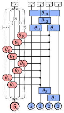
Figure E5: Variational ansatz for simulating a single plaquette with open boundary condition when the gauge field is represented by a ququint. The gates used in the circuit are defined in Appendix D1.

The results are even more striking in the case of a pure gauge theory as discussed in Fig. 2 of the main text. Here, the qudit platform shows no scaling with gauge field truncation, as the added complexity is only in the local qudit operations. In the qubit platform, on the other hand, the gate count scales as $48+12d$, and the register size scales as $3d$, see Tab. E2. Considering an encoding optimized for register size, this growth can be reduced to $3\lceil\log_{2}(d)\rceil$, at the cost of a gate count that scales in general quadratically with the dimension.

	Qudit encoding			Qubit encoding
dimension $d$	3	5	7	3	5	7
register size	3	3	3	9	15	21
CNOT count	8	8	8	84	108	132
CNOT fidelity	99%
approx. circ. fid.	92%	92%	92%	43%	34%	27%
CNOT fidelity	99.5%
approx. circ. fid.	96%	96%	96%	66%	58%	52%

Table E2: Circuit complexity of a pure gauge plaquette with periodic boundary conditions. The complexity is measured in a hardware-agnostic way by the gate count when all entangling gates (qubit and qudit) are decomposed into two-level CNOT gates under the assumption that these gates work equally well in qudit as in qubit systems. More efficient decompositions might exist by using custom hardware-efficient gates.

Finally, one might suspect that the price to pay for the reduced circuit complexity in the qudit approach is a less favorable runtime. While it is generally true that the qudit circuits take longer due to long readout times, we show in Tab. E3 that even the tradeoff between qudit readout ($(d-2)4$ ms) and qubit gate complexity ($0.2$ ms per gate) is slightly in favor of the qudit system for the problems studied here.

	Qudit encoding			Qubit encoding
dimension $d$	3	5	7	3	5	7
register size	3	3	3	9	15	21
rel. runtime open	1	1.52	2.04	1.48	2.26	3.04
rel. runtime periodic	1	1.54	2.08	1.76	2.08	2.41

Table E3: Runtimes of one execution of the qubit and qudit implementations. These times are calculated for the device used in the main text and may differ in other architectures.

Appendix F VQE circuit for pure-gauge QED with periodic boundary conditions

We give here the essential points of the design of the circuit used to study the pure-gauge QED model producing the results shown in Fig. 2d. A more detailed discussion is found in Ref. Paulson et al. (2021).

As for the case of 2D-QED with matter discussed in the main text, the form of the circuit is inspired by the Hamiltonian that the VQE solves, providing us with a scalable strategy that works also for higher truncations of the gauge field, and also with two different variational circuits for the electric and magnetic representation respectively. Let us consider the electric Hamiltonian given in Eqs. (C11), which is solved by the circuit given in Fig. 2c. After creating superpositions of all states for rotator $\hat{R}_{2}$, there is a layer of C-ROT gates that reflects the coupling between rotators given by $\hat{H}^{(e)}_{E}$, where we have used the symmetry between rotator $\hat{R}_{1}$ and $\hat{R}_{3}$ to reduce the number of independent variational parameters. For larger values of $g^{-2}$, the system tends to occupy states where the three rotators occupy the same electric field eigenstate, therefore we spread the population of rotators 1 and 3 controlling suitably on the corresponding state of rotator 2.

The circuit for the magnetic Hamiltonian given in Eqs. (C13) and depicted in Fig. F6 is designed with similar arguments.

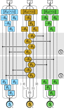
Figure F6: Variational circuit for the magnetic representation for the qutrit (solid lines) and the ququint (all, except box marked with qutrit) truncation. The explicit form of the gates employed is given in Appendix D1. The last gate in the circuit is defined as $R_{Z}(\theta)=\exp\left(-i\theta Z\right)$, where $Z=\operatorname{diag}(-1,0,1)$ for the qutrit, and $Z=\operatorname{diag}(-2,-1,0,1,2)$ for the ququint truncation.

Appendix G Experimental details

G1 Optimal encoding and cross-talk suppression

In circuits with embedded C-ROTs the choice of the qudit encoding requires careful treatment of the frequency spectrum and the structure of the quantum circuit to optimize the encoding of qudits in trapped ions. From the pure gauge variational ququint circuit shown in Fig. 2c, it is evident that only few states participate in the C-ROTs, namely $\ket{\pm 2}$ of control qudit and $\ket{0}$, $\ket{\pm 1}$ of the two target qudits. Optimal encoding yields the strongest coupling of the qudit states with the auxiliary ground state $\ket{g}$ on the blue sideband while simultaneously minimizing accumulating phase errors as a consequence of imperfect AC Stark shift compensation. The latter is achieved by restricting transitions, which lead to large Stark shifts, to static angles of $\pm\pi$, making the shift constant and easier to compensate. Figure G7 shows the chosen encodings for control and target qudits for the ququint circuit shown in Fig. 2c for the electric representation. The states with the largest coupling to $\ket{g}$ are highlighted in blue. Note, that in the magnetic representation, a different encoding is chosen.

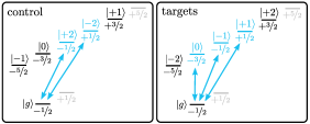
Figure G7: Optimal encodings of control and target qudits in the $D_{\nicefrac{{5}}{{2}}}$ manifold of ${}^{40}\mathrm{Ca}^{+}$ applied for the pure gauge ququint circuit in Fig. 2c – the encoding is chosen such that relevant states for the C-ROTs have the strongest coupling to the blue sideband. We seek to minimize phase errors by allowing only $\pi$ rotations on all transitions, which induce large Stark shifts on the spectator levels.

The pure-gauge qutrit circuit can be constructed in such a way that spatially neighboring ions store the qutrit in different sets of Zeeman levels, with each set separated by frequencies of a few $\mathrm{MHz}$. Assigning integers to each ions in the string from left to right, ions with even indices encode the qutrit in Zeeman states with positive magnetic quantum numbers $\ket{-1^{\prime}}=D_{+\nicefrac{{1}}{{2}}}$, $\ket{0^{\prime}}=D_{+\nicefrac{{3}}{{2}}}$ and $\ket{+1^{\prime}}=D_{+\nicefrac{{5}}{{2}}}$, coupled via the second ground state $\ket{g^{\prime}}=S_{+\nicefrac{{1}}{{2}}}$ as shown in Fig. G8. With this spectroscopic decoupling scheme, next-neighbor cross-talk is effectively eliminated Meth et al. (2022) and higher axial trap frequencies can be used. However, spectroscopic decoupling is not possible for ququints, as no bi-partition of the $D_{\nicefrac{{5}}{{2}}}$ manifold exists in ${}^{40}\mathrm{Ca}^{+}$ for qudits of dimension $d>3$; here one would require different ion species or isotopes to apply this scheme.

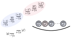
Figure G8: Next-neighbor cross-talk suppression in qutrits by proper choice of encoding – spatially neighboring ions encode the qutrit in different sets of Zeeman states with each set separated by a few $\mathrm{MHz}$. This encoding pattern is well suited to suppress cross-talk Meth et al. (2022), allowing higher axial trap frequencies, reducing the inter-ion distance.

A second approach to reduce next-neighbor cross-talk is to increase the spatial separation between ions encoding the qudits. This can be achieved in two ways, either lowering the axial confinement by reducing the end-cap voltage of the ion trap or by introducing additional buffer ions, which are transferred to a hidden state which does not couple with the laser pulses driving the actual quantum circuit. The former strategy is less suited for our specific circuits due to significant crowding of the mode spectrum, making it difficult to faithfully implement the CROT operations. Thus, for the $d=5$ pure gauge circuit as well as the gauge-matter circuit we chose the second method and introduced a pair of extra ions - in the pure gauge circuits, these buffers are located between each qudit, while the open plaquette circuit requires a buffer between each of the matter qubits, while we order the ion string in such a way that the gauge field qudit is physically located in the center of the string as shown in Fig. Fig. G9. This re-ordering ensures optimal performance of the Mølmer-Sørensen gates on the matter qubits at the very end of the circuit.

Figure G9: Artificially increasing the inter-qudit distance by introducing buffer ions. Buffer ions do not contribute to the circuit and do not couple with the light fields used to control the qudits. This strategy is employed for the $d=5$ pure gauge system as well as the circuits describing dynamical matter. For the latter case, we also chose to re-order the qudits inside the ion string to enhance the performance of the Mølmer-Sørensen entangling gates.

Additionally, to the two approaches presented in this section, we also employ composite rotations Meth et al. (2022) when bringing the buffer ions to their hidden state.

G2 Gate count optimization

The structure of the quantum circuits enables us to implement shortcuts, reducing the number of entangling gates; these shortcuts are best explained by the circuit in Fig. 1d. First, if the input state of one of the qudits is known, the number of interactions with the phonon mode $B(\theta,\phi)$ can be reduced to $n_{\mathrm{B(\theta,\phi)}}=2$ compared to the general case of a C-ROT being composed of $n_{B(\theta,\phi)}=5$ BSB pulses. This strategy is applied to the matter qubits in the gauge-matter-circuit for the angles $\theta_{1}$, $\theta_{2}$ and $-\theta_{7}$, where the state of the ‘left’ qubit entering each operation is exactly known. Second, if two C-ROTs are executed successively on the same control state as it would be for the pairs $(\theta_{3},\theta_{4})$ and $(\theta_{5},\theta_{6})$ in Fig. 1d, two successive $B(\theta,\phi)$ cancel out as it can be imagined by extending the sequence in Fig. A2 by a second C-ROT. Third, we implement the SWAP operations with angles $\theta_{7}$, $\theta_{8}$ and $\theta_{9}$ by sequences of three Mølmer-Sørensen (MS) gates Sørensen and Mølmer (1999) and local single-qubit rotations, which, in this case, is more favorable than the blue-sideband approach in terms of gate count.

G3 Measurement and readout of qudits

Measurements on a qudit with dimension $d$ are implemented by a series of single-qudit operations followed by a sequence of $d-1$ detection events and local $\pi$ rotations. Our optimal encoding of the qudits requires an additional reordering of the quantum states to match a $W$-pattern as shown in Fig. G10. In this arrangement any state $\ket{i}$ directly couples with $\ket{i\pm 1}$, which enables a straightforward QR-decomposition-based compilation of the measurement operator into a sequence of single qudit rotations.

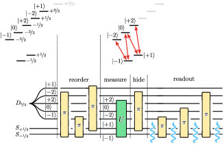
Figure G10: Measurement and readout of a ququint – the ququint is initially encoded in the $D_{\nicefrac{{5}}{{2}}}$ manifold of ${}^{40}\mathrm{Ca}^{+}$ similar to Fig. G7 (left). It is then reordered by a sequence of $\pi$-pulses, such that the states are arranged in the shape of the letter W (right). The coupling between states $\ket{i\pm 1}\leftrightarrow\ket{i}$ is required to faithfully implement the measurement operation $U$ in green. After hiding $\ket{+1}$ in the $D_{\nicefrac{{5}}{{2}}}$ manifold, the readout sequence is executed as a series of detection and re-cooling & optical pumping pulses indicated by blue arrows. Additional $\pi$-pulses rotate the desired state to the ground state manifold, such that photons can be scattered on the short-lived $S_{\nicefrac{{1}}{{2}}}\leftrightarrow P_{\nicefrac{{1}}{{2}}}$ transition.

After the measurement operation has been applied, the readout is implemented by a sequence of $d-2$ local $\pi$-flips and $d-1$ detection events. Each event is composed of a $1~{}\mathrm{ms}$ window, during which the fluorescence of each ion is recorded on a sensitive EMCCD camera, followed by $2~{}\mathrm{ms}$ of Doppler cooling and $0.5~{}\mathrm{ms}$ of polarization gradient cooling; this re-cooling pattern is not required after the last detection. We mention, that the duration of the readout in our experiment scales as $\approx(d-2)\cdot 3.5~{}\mathrm{ms}+1~{}\mathrm{ms}$ for any qudit dimension $d$ – this is on the order of the duration of the ground state cooling sequence at the beginning of each experiment run.

Appendix H Noise Model

While systems consisting of qubits only can often be accurately described by generic noise models such as simple depolarising noise, we found that for our qudit systems this is too reductive. Therefore, we construct a more realistic noise model based on the physics of how the gates of our circuits are realized. In particular, our heuristic model includes imperfect precision in the variational parameters and dephasing of the prepared quantum state. We find good agreement between the experimental results and the simulated data.

Amplitude fluctuations. We expect that the precision in the gate angles we aim to apply throughout the experiment suffers from fluctuations of the addressing laser amplitude. A gate $\hat{U}(\theta)$ is hence replaced by $\hat{U}(\theta+\delta\theta)$, where $\delta\theta$ is a stochastic variable extracted from a Gaussian $\mathcal{N}(0,\sigma_{\text{a}})$ with mean $\mu=0$ and variance $\sigma_{\text{a}}$.

Phase errors. In trapped ion systems, while single qudit operations can be carried out with a fidelity close to unity, two-qudit entangling gates and controlled excitation of the ions’ motion are the dominant sources of errors. C-ROT operations in qudits introduce phase noise due to AC Stark shifts of different magnitude: (1) exciting the motion on a chosen control state $\ket{i}$ introduces a (small) phase error $\phi_{i}$ on that state due to imperfect compensation and (2) spectator states that are not involved in the interaction ($\ket{j}$, with $j\neq i$) accumulate a phase $\Phi_{j}$ due to imperfect compensation of AC stark shifts. Each C-ROT is a composition of single qudit operations as shown in Fig. A2—for any blue sideband operation exciting the motion via the state $\ket{i}$, we identify the mapping $c_{i}\ket{i}+\sum_{j\neq i}c_{j}\ket{j}\mapsto e^{i\phi_{i}}c_{i}\ket{i}+\sum_{j\neq i}e^{i\Phi_{j}}c_{j}\ket{j}$. As such, the control qudit is mapped to the state in Eq. (H17), while the target acquires phases according to Eq. (H18).

$$c_{i}\ket{i}+\sum_{j\neq i}c_{j}\ket{j}\mapsto e^{i2\phi_{i}}c_{i}\ket{i}+\sum_{j\neq i}e^{i2\Phi_{j}}c_{j}\ket{j}$$ (H17)

$$\begin{split}&c_{i}\ket{i}+c_{j}\ket{j}+\sum_{k\neq i,j}c_{k}\ket{k}\mapsto\\ &e^{i(2\phi_{i}+\Phi_{i})}c_{i}\ket{i}+e^{i(2\Phi_{j}+\phi_{j})}c_{j}\ket{j}+c_{k}\sum_{k\neq i,j}e^{i3\Phi_{k}}\ket{k}\end{split}$$ (H18)

The second-beam technique Häffner et al. (2008) applied to cancel the AC Stark shift on the actively driven transition $\ket{g}\leftrightarrow\ket{i}$ is robust to intensity noise, as both beams are affected equally by fluctuations. Thus, the phase error $\phi_{i}$ is considered to be small compared to $\Phi_{j}$ and can be neglected for simplicity. Furthermore, we make the simplifying assumption that the passively (in software) compensated spectator shifts yield the same phase error for all levels $\Phi_{j}\mapsto\Phi$, and thus the mappings simplify to Eq. (H19) and Eq. (H20).

$$c_{i}\ket{i}+\sum_{j\neq i}c_{j}\ket{j}\mapsto c_{i}\ket{i}+e^{i2\Phi}\sum_{j\neq i}c_{j}\ket{j}$$ (H19)

$$\begin{split}&c_{i}\ket{i}+c_{j}\ket{j}+\sum_{k\neq i,j}c_{k}\ket{k}\mapsto\\ &e^{i\Phi}c_{i}\ket{i}+e^{i2\Phi}c_{j}\ket{j}+e^{i3\Phi}\sum_{k\neq i,j}c_{k}\ket{k}\end{split}$$ (H20)

Consecutive C-ROTs controlled by the same qudit and same state (see for example circuit in Fig. 2c) can be contracted, reducing the number of blue sideband pulses. For target qutrits, we deduce the pattern

$$e^{i3\Phi}c_{-1}\ket{-1}+e^{i2\Phi}c_{0}\ket{0}+e^{i3\Phi}c_{+1}\ket{+1},$$ (H21)

while for ququints we find

$$\begin{split}&e^{i3\Phi}c_{-2}\ket{-2}+e^{i3\Phi}c_{-1}\ket{-1}+e^{i2\Phi}c_{0}\ket{0}+\\ &e^{i\Phi}c_{+1}\ket{+1}+e^{i2\Phi}c_{+2}\ket{+2}.\end{split}$$ (H22)

We model the phase error $\Phi$ with a Gaussian distribution $\mathcal{N}(0,\sigma_{\text{p}})$ with mean $\mu=0$ and variance $\sigma_{\text{p}}$.

Results. In Fig. H11 we compare the experimental VQE results with simulated data for the open plaquette (first column) and for the pure gauge theory (second column). In the latter case the blue (orange) markers correspond to the electric (magnetic) representation. For the simulation, we consider variational parameters obtained without noise, and we calculate the expectation values of the relevant observables when the variational circuit is affected by the noise with parameters estimated as $\sigma_{\text{a}}=0.022$, $\sigma_{\text{p}}=0.36$. We can see good qualitative agreement between the experimental and the simulated data. In particular, in the case of QED with matter, while the energy obtained experimentally can be above the exact first excited energy level, we can see from the plaquette expectation value that the ground state properties are correctly obtained.

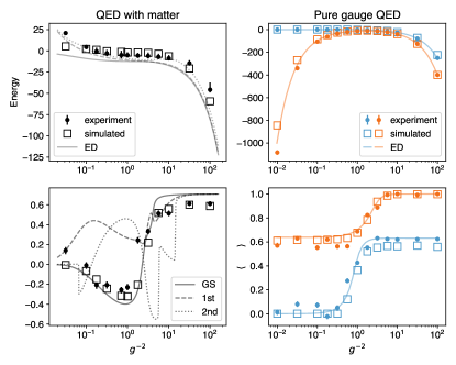
Figure H11: Simulated noise model for the experiment. Energy (first row) and plaquette expectation value (second row) for the two models studied via experimental VQE, namely 2D-QED with matter (first column), and an instance of pure gauge 2D-QED (second column). For the pure gauge model, blue (orange) lines and markers correspond to the simulations performed with the electric (magnetic) representation. After obtaining variational parameters in the absence of noise, the simulated noisy data (squares) is obtained via the noise model detailed in the text, which includes amplitude fluctuations and phase errors. The results from experimental quantum computations (dots) show good agreement with the simulated noisy data. As a reference, we plot as lines the results for the ground state from an exact diagonalization, and for the plaquette with matter we also plot the observables for the first and second excited state. While the energy obtained experimentally can be above the exact first excited energy level, we can see from the plaquette expectation value that the ground state properties are correctly obtained.

References

- Ahn et al. (2000) J. Ahn, T. Weinacht, and P. Bucksbaum, Science 287, 463 (2000).
- Godfrin et al. (2017) C. Godfrin, A. Ferhat, R. Ballou, S. Klyatskaya, M. Ruben, W. Wernsdorfer, and F. Balestro, Phys. Rev. Lett. 119, 187702 (2017).
- Anderson et al. (2015) B. E. Anderson, H. Sosa-Martinez, C. A. Riofrío, I. H. Deutsch, and P. S. Jessen, Phys. Rev. Lett. 114, 240401 (2015).
- Morvan et al. (2021) A. Morvan, V. V. Ramasesh, M. S. Blok, J. M. Kreikebaum, K. O’Brien, L. Chen, B. K. Mitchell, R. K. Naik, D. I. Santiago, and I. Siddiqi, Phys. Rev. Lett. 126, 210504 (2021).
- Senko et al. (2015) C. Senko, P. Richerme, J. Smith, A. Lee, I. Cohen, A. Retzker, and C. Monroe, Phys. Rev. X 5, 021026 (2015).
- Wang et al. (2018) J. Wang, S. Paesani, Y. Ding, R. Santagati, P. Skrzypczyk, A. Salavrakos, J. Tura, R. Augusiak, L. Mančinska, D. Bacco, D. Bonneau, J. W. Silverstone, Q. Gong, A. Acín, K. Rottwitt, L. K. Oxenløwe, J. L. O’Brien, A. Laing, and M. G. Thompson, Science 360, 285 (2018).
- Chen et al. (2021) W. Chen, J. Gan, J.-N. Zhang, D. Matuskevich, and K. Kim, Chinese Physics B 30, 060311 (2021).
- Wang et al. (2020) Y. Wang, Z. Hu, B. C. Sanders, and S. Kais, Front. Phys. 8 (2020).
- Ringbauer et al. (2022) M. Ringbauer, M. Meth, L. Postler, R. Stricker, R. Blatt, P. Schindler, and T. Monz, Nat. Phys. 18, 1053 (2022).
- Cirac and Zoller (1995) J. I. Cirac and P. Zoller, Phys. Rev. Lett. 74, 4091 (1995).
- Kuzmin and Silvi (2020) V. V. Kuzmin and P. Silvi, Quantum 4, 290 (2020).
- Meth et al. (2022) M. Meth, V. Kuzmin, R. van Bijnen, L. Postler, R. Stricker, R. Blatt, M. Ringbauer, T. Monz, P. Silvi, and P. Schindler, Phys. Rev. X 12, 041035 (2022).
- Cao et al. (2019) Y. Cao, J. Romero, J. P. Olson, M. Degroote, P. D. Johnson, M. Kieferová, I. D. Kivlichan, T. Menke, B. Peropadre, N. P. D. Sawaya, S. Sim, L. Veis, and A. Aspuru-Guzik, Chem. Rev. 119, 10856 (2019).
- MacDonell et al. (2021) R. J. MacDonell, C. E. Dickerson, C. J. T. Birch, A. Kumar, C. L. Edmunds, M. J. Biercuk, C. Hempel, and I. Kassal, Chem. Sci. 12, 9794 (2021).
- Maskara et al. (2023) N. Maskara, J. Shee, S. Ostermann, A. M. Gomez, R. A. Bravo, D. Wang, M. P. Head-Gordon, S. F. Yelin, and M. D. Lukin, in Bulletin of the American Physical Society (American Physical Society, 2023).
- Haldane (1983) F. D. M. Haldane, Phys. Rev. Lett. 50, 1153 (1983).
- Sawaya et al. (2020) N. P. D. Sawaya, T. Menke, T. H. Kyaw, S. Johri, A. Aspuru-Guzik, and G. G. Guerreschi, NPJ Quantum Inf. 6, 49 (2020).
- Aoki et al. (2022) Y. Aoki, T. Blum, G. Colangelo, S. Collins, M. D. Morte, P. Dimopoulos, S. Dürr, X. Feng, H. Fukaya, M. Golterman, S. Gottlieb, R. Gupta, S. Hashimoto, U. M. Heller, G. Herdoiza, P. Hernandez, R. Horsley, A. Jüttner, T. Kaneko, E. Lunghi, S. Meinel, C. Monahan, A. Nicholson, T. Onogi, C. Pena, P. Petreczky, A. Portelli, A. Ramos, S. R. Sharpe, J. N. Simone, S. Simula, S. Sint, R. Sommer, N. Tantalo, R. Van de Water, U. Wenger, H. Wittig, and Flavour Lattice Averaging Group (FLAG), Eur. Phys. J. C 82, 869 (2022).
- Gattringer and Langfeld (2016) C. Gattringer and K. Langfeld, Int. J. Mod. Phys. A 31, 1643007 (2016).
- Robaina et al. (2021) D. Robaina, M. C. Bañuls, and J. I. Cirac, Phys. Rev. Lett. 126, 050401 (2021).
- Banuls et al. (2019) M. C. Banuls, K. Cichy, J. I. Cirac, K. Jansen, and S. Kühn, PoS Proc. Sci. Lattice 2018, 022 (2019).
- Hackett et al. (2019) D. C. Hackett, K. Howe, C. Hughes, W. Jay, E. T. Neil, and J. N. Simone, Phys. Rev. A 99, 062341 (2019).
- Haase et al. (2021) J. F. Haase, L. Dellantonio, A. Celi, D. Paulson, A. Kan, K. Jansen, and C. A. Muschik, Quantum 5, 393 (2021).
- Bauer and Grabowska (2023) C. W. Bauer and D. M. Grabowska, Phys. Rev. D 107, L031503 (2023).
- Yang et al. (2016) D. Yang, G. S. Giri, M. Johanning, C. Wunderlich, P. Zoller, and P. Hauke, Phys. Rev. A 94, 052321 (2016).
- Mil et al. (2020) A. Mil, T. V. Zache, A. Hegde, A. Xia, R. P. Bhatt, M. K. Oberthaler, P. Hauke, J. Berges, and F. Jendrzejewski, Science 367, 1128 (2020).
- González-Cuadra et al. (2022) D. González-Cuadra, T. V. Zache, J. Carrasco, B. Kraus, and P. Zoller, Phys. Rev. Lett. 129, 160501 (2022).
- Martinez et al. (2016) E. A. Martinez, C. A. Muschik, P. Schindler, D. Nigg, A. Erhard, M. Heyl, P. Hauke, M. Dalmonte, T. Monz, P. Zoller, et al., Nature 534, 516 (2016).
- Meglio et al. (2023) A. D. Meglio, K. Jansen, I. Tavernelli, C. Alexandrou, S. Arunachalam, C. W. Bauer, K. Borras, S. Carrazza, A. Crippa, V. Croft, R. de Putter, A. Delgado, V. Dunjko, D. J. Egger, E. Fernandez-Combarro, E. Fuchs, L. Funcke, D. Gonzalez-Cuadra, M. Grossi, J. C. Halimeh, Z. Holmes, S. Kuhn, D. Lacroix, R. Lewis, D. Lucchesi, M. L. Martinez, F. Meloni, A. Mezzacapo, S. Montangero, L. Nagano, V. Radescu, E. R. Ortega, A. Roggero, J. Schuhmacher, J. Seixas, P. Silvi, P. Spentzouris, F. Tacchino, K. Temme, K. Terashi, J. Tura, C. Tuysuz, S. Vallecorsa, U.-J. Wiese, S. Yoo, and J. Zhang, “Quantum Computing for High-Energy Physics: State of the Art and Challenges. Summary of the QC4HEP Working Group,” (2023), arXiv:2307.03236 [quant-ph] .
- Klco et al. (2020) N. Klco, M. J. Savage, and J. R. Stryker, Phys. Rev. D 101, 074512 (2020).
- Ciavarella et al. (2021) A. Ciavarella, N. Klco, and M. J. Savage, Phys. Rev. D 103, 094501 (2021).
- A Rahman et al. (2021) S. A Rahman, R. Lewis, E. Mendicelli, and S. Powell, Phys. Rev. D 104, 034501 (2021).
- Ciavarella and Chernyshev (2022) A. N. Ciavarella and I. A. Chernyshev, Phys. Rev. D 105, 074504 (2022).
- A Rahman et al. (2022) S. A Rahman, R. Lewis, E. Mendicelli, and S. Powell, Phys. Rev. D 106, 074502 (2022).
- Rahman et al. (2022) S. A. Rahman, R. Lewis, E. Mendicelli, and S. Powell, “Real time evolution and a traveling excitation in SU(2) pure gauge theory on a quantum computer,” (2022), arXiv:2210.11606 [hep-lat] .
- Ciavarella (2023) A. N. Ciavarella, “Quantum Simulation of Lattice QCD with Improved Hamiltonians,” (2023), arXiv:2307.05593 [hep-lat] .
- Creutz et al. (1983) M. Creutz, L. Jacobs, and C. Rebbi, Phys. Rep. 95, 201 (1983).
- Aoki et al. (2017) S. Aoki, Y. Aoki, C. Bernard, T. Blum, G. Colangelo, M. Della Morte, S. Dürr, A. X. El-Khadra, H. Fukaya, R. Horsley, et al., Eur. Phys. J. C 77, 112 (2017).
- Aoki et al. (2020) S. Aoki, Y. Aoki, D. Bečirević, T. Blum, G. Colangelo, S. Collins, M. Della Morte, P. Dimopoulos, S. Dürr, H. Fukaya, et al., Eur. Phys. J. C 80, 1 (2020).
- Farhi et al. (2014) E. Farhi, J. Goldstone, and S. Gutmann, “A quantum approximate optimization algorithm,” (2014), arXiv:1411.4028 [quant-ph] .
- Peruzzo et al. (2014) A. Peruzzo, J. McClean, P. Shadbolt, M.-H. Yung, X.-Q. Zhou, P. J. Love, A. Aspuru-Guzik, and J. L. O’brien, Nat. Comm. 5, 1 (2014).
- McClean et al. (2016) J. R. McClean, J. Romero, R. Babbush, and A. Aspuru-Guzik, New J. Phys. 18, 023023 (2016).
- Kogut and Susskind (1975) J. Kogut and L. Susskind, Phys. Rev. D 11, 395 (1975).
- Clemente et al. (2022) G. Clemente, A. Crippa, and K. Jansen, Phys. Rev. D 106, 114511 (2022).
- Jordan and Wigner (1928) P. Jordan and E. P. Wigner, Z. Phys. 47, 631 (1928).
- Paulson et al. (2021) D. Paulson, L. Dellantonio, J. F. Haase, A. Celi, A. Kan, A. Jena, C. Kokail, R. van Bijnen, K. Jansen, P. Zoller, and C. A. Muschik, PRX Quantum 2, 030334 (2021).
- (47) A. Jena et al., In preparation.
- Nguyen et al. (2022) N. H. Nguyen, M. C. Tran, Y. Zhu, A. M. Green, C. H. Alderete, Z. Davoudi, and N. M. Linke, PRX Quantum 3, 020324 (2022).
- Kan et al. (2021) A. Kan, L. Funcke, S. Kühn, L. Dellantonio, J. Zhang, J. F. Haase, C. A. Muschik, and K. Jansen, Phys. Rev. D 104, 034504 (2021).
- Zohar (2021) E. Zohar, Philos. Trans. R. Soc. A 380, 20210069 (2021).
- Kim et al. (2008) S. Kim, R. R. Mcleod, M. Saffman, and K. H. Wagner, Appl. Opt. 47, 1816 (2008).
- Häffner et al. (2003) H. Häffner, S. Gulde, M. Riebe, G. Lancaster, C. Becher, J. Eschner, F. Schmidt-Kaler, and R. Blatt, Phys. Rev. Lett. 90, 143602 (2003).
- Hamer et al. (1997) C. Hamer, Z. Weihong, and J. Oitmaa, Phys. Rev. D 56, 55 (1997).
- Gard et al. (2020) B. T. Gard, L. Zhu, G. S. Barron, N. J. Mayhall, S. E. Economou, and E. Barnes, NPJ Quantum Inf. 6, 10 (2020).
- Frazier (2018) P. I. Frazier, “A tutorial on bayesian optimization,” (2018), arXiv:1807.02811 [stat.ML] .
- Eriksson et al. (2019) D. Eriksson, M. Pearce, J. Gardner, R. D. Turner, and M. Poloczek, in Advances in Neural Information Processing Systems, Vol. 32, edited by H. Wallach, H. Larochelle, A. Beygelzimer, F. d'Alché-Buc, E. Fox, and R. Garnett (Curran Associates, Inc., 2019).
- Shlosberg et al. (2023) A. Shlosberg, A. J. Jena, P. Mukhopadhyay, J. F. Haase, F. Leditzky, and L. Dellantonio, Quantum 7, 906 (2023).
- Gottesman (1999) D. Gottesman, in Quantum Computing and Quantum Communications: First NASA International Conference, QCQC’98 Palm Springs, California, USA February 17–20, 1998 Selected Papers (Springer, 1999) pp. 302–313.
- Sørensen and Mølmer (1999) A. Sørensen and K. Mølmer, Phys. Rev. Lett. 82, 1971 (1999).
- Häffner et al. (2008) H. Häffner, C. F. Roos, and R. Blatt, Phys. Rep. 469, 155 (2008).