Black-Box Training Data Identification in GANs via Detector Networks

Abstract

Since their inception Generative Adversarial Networks (GANs) have been popular generative models across images, audio, video, and tabular data. In this paper we study whether given access to a trained GAN, as well as fresh samples from the underlying distribution, if it is possible for an attacker to efficiently identify if a given point is a member of the GAN’s training data. This is of interest for both reasons related to copyright, where a user may want to determine if their copyrighted data has been used to train a GAN, and in the study of data privacy, where the ability to detect training set membership is known as a membership inference attack. Unlike the majority of prior work this paper investigates the privacy implications of using GANs in black-box settings, where the attack only has access to samples from the generator, rather than access to the discriminator as well. We introduce a suite of membership inference attacks against GANs in the black-box setting and evaluate our attacks on image GANs trained on the CIFAR10 dataset and tabular GANs trained on genomic data. Our most successful attack, called The Detector, involve training a second network to score samples based on their likelihood of being generated by the GAN, as opposed to a fresh sample from the distribution. We prove under a simple model of the generator that the detector is an approximately optimal membership inference attack. Across a wide range of tabular and image datasets, attacks, and GAN architectures, we find that adversaries can orchestrate non-trivial privacy attacks when provided with access to samples from the generator. At the same time, the attack success achievable against GANs still appears to be lower compared to other generative and discriminative models; this leaves the intriguing open question of whether GANs are in fact more private, or if it is a matter of developing stronger attacks.

1 Introduction

Beginning in 2014 with the seminal paper  [1], until the recent emergence of diffusion models  [2, 3, 4, 5], generative adversarial networks (GANs) have been the dominant generative model across image, audio, video, and tabular data generation  [6, 7, 8, 9, 10, 11], and are still in some cases competitive with diffusion models, for example in [12, 13, 14, 15]. One promising use case of generative models is when the underlying training data is private, and so there are restrictions on sharing the data with interested parties. Rather than sharing the data directly, after training a generative model $G$ on the private data, either $G$ can be shared directly, or a new synthetic dataset can be generated from $G$, which can be used for downstream tasks without sharing the underlying data. While this seems private on the surface, a line of work has shown that sharing access to a generative model or synthetic dataset may leak private information from the underlying training data  [16, 17]. Recent work  [18] has shown that as compared to GANs, diffusion models are far less private, memorizing as much as $5\times$ more of their training data, and as a result are highly susceptible to attacks that can reconstruct the underlying training data. These considerations make GANs a more natural choice of generative model for highly sensitive data – or do they?

Most existing work probing the privacy properties of GANs has typically focused on the "white-box" setting, where an adversary has access to the discriminator of the GAN, and is able to use standard techniques to conduct membership inference attacks based on the loss  [16]; a notable exception is [19]. While these white-box attacks demonstrate releasing the discriminator in particular leaks information about the underlying training set, they are unsatisfying from a practical perspective, since typically only the generator would be shared after training. This raises a natural question about the privacy of GANs:

In the black-box setting where an adversary only has sample access to the generator, are effective privacy attacks possible?

Another potential motivation for developing efficient methods to determine whether a point was used to train a GAN comes from copyright. Suppose the creator of an image for example, suspects that their image was used in the training set of a generative model without their permission. Since the vast majority of state-of-the-art generative models are only made available via access to the generator, applying a black-box membership inference attack is the only way the creator can argue it is (statistically) likely their image was part of the training set. We address this gap by developing a battery of membership inference attacks against GANs that only require access to generated samples. We evaluate our attacks on target GANs trained on image and tabular data, focusing on image GANs trained on the popular CIFAR10 dataset  [20], and on tabular GANs trained on SNP (Single Nucleotide Polymorphisms  [21]) data from two popular genomic databases  [22, 23]. We selected genomic data because of the obvious underlying privacy concerns, and because of the high-dimensionality of the data, which makes the setting more challenging from a privacy perspective. Early privacy attacks on genomic databases [24] led the NIH to take the extreme step of restricting access to raw genomic summary results computed on SNP datasets like dbGaP [22], although they later reversed course following scientific outcry.

Contributions.

In this work, we develop state-of-the-art privacy attacks against GANs under the realistic assumption of black-box access, and conduct a thorough empirical investigation across $2$ GAN architectures trained on $6$ different tabular datasets created by sub-sampling $2$ genomic data repositories, and $4$ GAN architectures trained to generate images from CIFAR-10. We develop a new attack, which we call the Detector (and its extended version called the Augmented Detector or ADIS ), that trains a second network to detect GAN-generated samples, and applies it to the task of membership inference. We also derive theoretical results (Theorem 4.1) that shed light on our attack performance. We compare our Detector-based methods to an array of distance and likelihood-based attacks proposed in prior work [16, 25, 26] which we are the first to evaluate with recent best practice metrics for MIAs [27]. Generally, we find that while privacy leakage from GANs seems to be lower than reported in prior work [25, 18] for other types of generative models, there does still appear to be significant privacy leakage even in the black-box setting. Moreover, this privacy-leakage as measured by the success of our MIAs seems to vary based on the type of GAN trained, as well as the dimension and type of the underlying training data. To our knowledge, we are the first to apply detectors for generated samples to the task of membership inference against generative models.

2 Related Work

Membership Inference Attacks or MIAs were defined by [24] for genomic data, and formulated by [28] against ML models. In membership inference, an adversary uses model access as well as some outside information to determine whether a candidate point $x$ is a member of the model training set. Standard MIAs typically exploit the intuition that a point $x$ is more likely to be a training point if the loss of the model evaluated at $x$ is small [29], or in the white-box setting where they have access to the model’s gradients, if the gradients are small [30], although other approaches that rely on a notion of self-influence [31] and distance to the model boundary have been proposed [32, 33]. The state of the art attack against discriminative classifiers, called LiRA [27], approximates the likelihood ratio of the loss when $x$ is in the training set versus not in the training set, training additional shadow models to sample from these distributions.

Assuming access to the discriminator’s loss, as in [25], loss-based attacks are easily ported over to GANs. However, given that the discriminator is not required to sample from the generator once training is finished, there is no practical reason to assume that the adversary has access to the discriminator. [25] find that by thresholding on the discriminator loss, TPR at FPR = $.2$ on DCGAN trained on CIFAR-10 is a little under $.4$ when the target GAN is trained for $100$ epochs, but goes up to almost $100\%$ after $200$ epochs, indicating severe over-fitting by the discriminator. When they employ a black-box attack, they are able to achieve TPR = $.37$ at FPR = $.2$. We note that this is a less than $2$x improvement over baseline, even in the presence of potentially severe over-fitting during training.

[34] propose a black-box attack on GANs trained on CIFAR-10 that is very similar to a distance-based attack. Their statistic samples from the GAN and counts the proportion of generated samples that fall within a given distance $\epsilon$ of the candidate point. In order to set $\epsilon$, they estimate the $1\%$ or $.1\%$ quantiles of distances to the generated GAN via sampling. Note that this assumes access to a set of candidate points $x_{i}$ rather than a single candidate point that may or may not be a training point, although a similar idea could be implemented using reference data. While their attacks were quite effective against VAEs and on the simpler MNIST dataset, the best accuracy one of their distance-based attacks achieves on CIFAR-10 is a TPR that is barely above $50\%$, at a massive FPR that is also close to $50\%$ (Figure $4$(c)) with their other distance-based method performing worse than random guessing. Relatedly,  [16] proposed a distance-based attack scheme based on minimum distance to a test sample. In  [16] the adversary has access to synthetic samples from the target GAN and synthetic samples from a GAN trained on reference data ($G_{ref}$). We follow this approach for distance-based attacks, which we discuss further in Section 4.2. The most closely related work to our detector methods is  [26] who propose a density-based model called DOMIAS (Detecting Overfitting for Membership Inference Attacks against Synthetic Data), which infers membership by targeting local overfitting of the generative models. Rather than train a detector network to classify whether samples are generated from the target GAN or the reference data, DOMIAS performs dimension reduction in order to directly estimate both densities, and then uses the ratio of the densities as a statistic for membership inference.

Related to our study of tabular GANs trained on genomic data,  [35] proposed the use of GANs for the synthesis of realistic artificial genomes with the promise of none to little privacy loss. The absence of privacy loss in the proposed model was investigated by measuring the extent of overfitting using the nearest neighbor adversarial accuracy (AAT_TS) and privacy score metrics discussed in  [36]. It should be noted that while overfitting is sufficient to allow an adversary to perform MI (and hence constitute a privacy loss), it is not a necessary prerequisite for the attack to succeed, as shown in the formal analysis presented in  [29].

There have been a handful of recent papers that propose black-box attacks against generative models, nearly all of which rely on the heuristic that if a point is “closer” to generated samples that to random points from the distribution, it is more likely to be a training point [34][16]. The most closely related work to our detector methods is  [26] who propose a density-based model called DOMIAS, which infers membership by targeting local over-fitting of the generative models. Rather than train a detector network to classify whether samples are generated from the target GAN or the reference data, DOMIAS performs dimension reduction in order to directly estimate both densities, and then uses the ratio of the densities as a statistic for membership inference. We implement many of these methods in our experiments section, and summarize them in more detail in Appendix B.4.

3 Preliminaries

Generative Adversarial Network(GANs). Given training data drawn from a distribution, $X_{T}\sim\mathcal{P}$, a generative model tries to approximate $\mathcal{P}$. Generative adversarial networks (GANs) are examples of generative models and have gained popularity for their ability to generate realistic samples across a range of domains  [37, 38, 39, 40, 41]. The basic GAN set-up consists of two players - the discriminator ($D^{\prime}$) and the generator ($\mathcal{G}$)- engaging in a minimax game  [42] with training objective given as:

$$\mathbb{E}_{\mathbf{x}\sim\mathcal{P}}[\log D^{\prime}(\mathbf{x})]+\mathbb{E}_{\mathbf{z}\sim p_{\mathbf{z}}(\mathbf{z})}[\log(1-D^{\prime}(G(\mathbf{z})))$$

The generator, $G$, takes latent noise, $z$, as an input and generates a sample as output, while the discriminator examines data samples (i.e, $\mathbf{x},\,\,\text{and}\,\,G(\mathbf{z})$) and tries to discriminate samples from the generator (i.e $G(\mathbf{z})$ ) from the real data samples (i.e $\mathbf{x}$). The generator’s target is to generate realistic samples that would fool the discriminator, while the discriminator tries to detect counterfeit samples from the generator [42]. The training objective is typically optimized by updating the generator and discriminator via simultaneous gradient ascent.

Throughout the paper we’ll let $\mathcal{T}$ be the distribution that samples a random point from $X_{T}$, $\mathcal{G}$ the distribution that samples a point from $G$, $\mathcal{M}=\frac{1}{2}\mathcal{G}+\frac{1}{2}\mathcal{P}$ be the mixture distribution of $\mathcal{G}$ and $\mathcal{P}$, which we will need to define our detector attack in Section 4.1, and $\mathcal{R}=\frac{1}{2}\mathcal{T}+\frac{1}{2}\mathcal{P}$ be the mixture distribution we evaluate our MIAs on. Given a point $x$ let $\mathcal{G}(x),\mathcal{P}(x)$ denote the respective probability densities evaluated at $x$.

Black-Box Setting.

Following convention, we assume that our black-box attacks have access to samples from $\mathcal{G}$ but not the weights of $G$ directly, access to details about how the GAN was trained (e.g. the architecture of course not the training samples), and fresh samples from the distribution $\mathcal{P}$ [28, 43, 44].

Attack Framework.

We adopt an attack framework similar to that used in countless papers on membership inference attacks against machine learning models [28, 45, 27]. The model developer samples a training set $X_{T}\sim\mathcal{P}$, and trains a GAN $G$ on $X_{T}$, $G\sim\text{Train}(X_{T})$. Now consider a membership inference attack (MIA) $\mathcal{A}$; draw $x^{\prime}\sim\mathcal{R}$ and send $x^{\prime}$ to $\mathcal{A}$. The membership inference attacker $\mathcal{A}$ receives the candidate point $x^{\prime}$ and then outputs a guess: $1$ if $x^{\prime}\in X_{T}$, $0$ if $x^{\prime}\not\in X_{T}$. Note that if $\mathcal{A}$ only receives $x^{\prime}$, then it is impossible for $\mathcal{A}$ to output a guess that has accuracy $>\frac{1}{2}$, since the marginal distribution on $x^{\prime}$ is always $\mathcal{P}$. Absent any additional information, for an fixed FPR $\alpha$, the TPR achieved by $\mathcal{A}$’s guess is always $\leq\alpha$. In the black-box setting $\mathcal{A}$ also receives black-box access to draw random samples from $\mathcal{G}$ and additional samples from $\mathcal{P}$. From the above discussion, any accuracy $\mathcal{A}$ is able to achieve that is better than a random guess must be due to the ability to infer if $x^{\prime}\in X_{T}$ through access to samples from $\mathcal{G}$. In practice, rather than an MIA $\mathcal{A}$ outputting a $1$ or $0$ guess, $\mathcal{A}$ will output a real-valued score $\mathcal{A}(x^{\prime})$ corresponding to how likely $x^{\prime}$ is to be in $X_{T}$. Then any threshold $\tau\in\mathbb{R}$ corresponds to an attack $\textbf{1}\{\mathcal{A}(x^{\prime})>\tau\}$, and varying $\tau$ traces out a receiver operating characteristic (ROC) curve of achievable FPR/TPRs [27].

Attack Evaluation Metrics.

Recent work [27, 46] argues the most meaningful way to evaluate a membership inference attack $\mathcal{A}$ is not to look at the overall accuracy, but to focus on what TPRs are achieveable at low FPRs, as this could correspond to a more realistic privacy violation: a small subset of the training data that model can identify with high confidence. Note that this correspond to large values of $\frac{\text{TPR}}{\text{FPR}}$ at small FPRs. We adopt this convention here, reporting the achievable TPR at fixed FPRs ($.001,.005,.01,.1$) for all of our attacks (Tables 3, 4). As in [27] we plot all our attack ROC curves on the log-log scale in order to visualize what is happening at low FPRs. We also report the AUCs for each ROC curve in order to provide a quick high-level summary of attack success, but again we regard such average summary statistics as less important than the $\frac{\text{TPR}}{\text{FPR}}$ statistics.

4 Attack Model Types

The attacks we study fall into two broad categories: (i) Detector-based attacks rely on training a second classifier to distinguish generator samples from reference data samples, and then using that classifier’s predicted probability of being generated by $\mathcal{G}$ as a proxy for training set membership (ii) Distance-based attacks compute the distance between the candidate point and samples from the generator and samples from the reference data, and predict the point is a training point if it is closer to generated samples. In Section 4.1 we outline the basic process of training the Detector, and define its augmented variant ADIS. We state theoretical results that characterize the performance of an optimal detector-based attack and show that under a simplified model where the generator learns the distribution subject to some mode collapse, detector-based attacks are approximately optimal MIAs. In Section 4.2 we define the distance-based attacks proposed in prior work that we evaluate our methods against. In our experiments we also compare against the DOMIAS attack proposed in [26] – we defer the details of our implementation to Appendix  B.4.

4.1 Detector-Based Attacks

Figure 1: The pipeline for training the Detector $D_{\theta}$.

The Detector is based on the premise that a network that can distinguish samples generated from the GAN from samples from the true distribution, can also distinguish training samples from the distribution. Specifically a network called the Detector ($D_{\theta}$) is trained to classify samples from the GAN as $1$, and samples from $\mathcal{P}$ as $0$. After training $D_{\theta}$, given a candidate point $x$, the membership inference score for $x$ is the predicted probability under $D_{\theta}$ of the point being generated from the GAN, which we’ll denote $D_{\theta}(x)$. The high-level pipeline for training $D_{\theta}$ is shown in Figure 1, with the algorithmic details of how to set the hyper-parameters deferred to the relevant experimental sections. The variant of the Detector attack we call the Augmented Detector (ADIS) follows the same process of training the Detector, but augments the feature space used to train the Detector with statistics based on the distance from $x$ to samples from the generator and reference data, including the DOMIAS statistic [26]. The full details of how we train ADIS are deferred to Appendix B.4.

Now let $f:\mathcal{X}\to[0,1]$, and $\text{Lip}(f)$ denote the Lipschitz constant of $f$. We can relate the error of $f$ when used for membership inference on points sampled from $\mathcal{R}$ to the error of $f$ when used to classify whether points from $\mathcal{M}$ were sampled from $\mathcal{G}$ or $\mathcal{P}$. If points sampled from $\mathcal{P}$ are labeled $0$ and points from $\mathcal{G}$ are labeled $1$, then the FPR of $f$ used to classify points from $\mathcal{M}$ is $\text{FPR}_{\mathcal{M}}=\frac{1}{2}\mathbb{E}_{\mathcal{P}}[f(x)]$. Now, the FPR of $f$ as an MIA is $\text{FPR}_{\mathcal{R}}=\mathbb{E}_{\mathcal{R}}[f(x)|x\in\mathcal{P}]=\text{FPR}_{\mathcal{M}}$, so the FPRs are the same. The TPR is more interesting; it is easy to show (Lemma A.1) that

$$\text{TPR}_{\mathcal{R}}(f)\leq\text{TPR}_{\mathcal{M}}(f)+\frac{\text{Lip}(f)}{2}W^{1}(\mathcal{G},\mathcal{T}),$$ (1)

where $W^{1}(\mathcal{G},\mathcal{T})$ is the $1$-Wasserstein distance between $\mathcal{G}$ and $\mathcal{T}$. Note that when $\mathcal{G}=\mathcal{T}$ then $\mathcal{R}=\mathcal{M}$, and the above inequality becomes equality, with $W^{1}(\mathcal{G},\mathcal{T})=0$. Equation 1 motivates the Detector attack, because although we can’t directly sample from $\mathcal{R}$, and therefore can’t train $f$ to maximize $\text{TPR}_{\mathcal{R}}(f)$ at a fixed FPR rate, in the black-box setting we can still sample from $\mathcal{M}$, and so we can train $f$ that maximizes $\text{TPR}_{\mathcal{M}}(f)$ subject to $\text{FPR}_{\mathcal{M}}(f)=\text{FPR}_{\mathcal{R}}(f)=\alpha$ for any $\alpha\in[0,1]$. While Equation 1 is nice in that we can upper bound the rate we’d expect $\text{TPR}_{\mathcal{R}}(f)\to\text{TPR}_{\mathcal{M}}(f)$ as $\mathcal{G}\to\mathcal{T}$, namely the rate $W^{1}(\mathcal{G},\mathcal{T})\to 0$, it doesn’t tell us much about why in practice a classifier $f$ that minimizes error on $\mathcal{M}$ might achieve low error on $\mathcal{R}$: (i) $f$ is a neural network and so $\text{Lip}(f)$ could be very large in practice, making Equation 1 vacuous and (ii) $W^{1}(\mathcal{G},\mathcal{T})$ can be quite large.

In Theorem 4.1 we prove the neat result that if $\mathcal{G}$ is a mixture of the training set distribution $\mathcal{T}$ and the dataset $\mathcal{P}$, and $f^{*}$ is the Bayes optimal classifier with respect to $\mathcal{M}$, then the MIA that thresholds based on $f^{*}$ achieves maximal TPR at any fixed FPR on the distribution $\mathcal{R}$. We defer the proof to the Appendix, which uses the form of $\mathcal{G}$ to decompose the error on $\mathcal{G}$ into errors on $\mathcal{T},\mathcal{P}$, and follows from the Neyman Pearson lemma [47] and the assumption that $f^{*}$ is Bayes optimal.

Theorem 4.1.

Suppose that $\mathcal{G}=\beta\mathcal{P}+(1-\beta)\mathcal{T}$ for some $\beta\in[0,1]$. Let $f^{*}:\mathcal{X}\to[0,1]$ be the posterior probability a sample from $\mathcal{M}$ is drawn from $\mathcal{G}:f^{*}(x)=\frac{\mathcal{G}(x)}{\mathcal{G}(x)+\mathcal{P}(x)}$. Then for any fixed $\alpha\in[0,1],\;\exists\tau_{\alpha}$ such that attack

$$F^{*}(x)=\textbf{1}\{f^{*}(x)>\tau_{\alpha}\}$$

satisfies $\text{FPR}_{\mathcal{R}}(F^{*})=\alpha$, and for any MIA $f$ such that $\text{FPR}_{\mathcal{R}}(f)=\alpha$, $\text{TPR}_{\mathcal{R}}(f)\leq\text{TPR}_{\mathcal{R}}(F^{*})$.

Proof.

Let $f:\mathcal{X}\to\{0,1\}$ be an arbitrary MIA achieving FPR $\alpha$, that is $\mathbb{E}_{x\sim\mathcal{D}}[f(x)]=\alpha$. Then the TPR of $f$ at distinguishing samples from $G$ is $\mathbb{E}_{x\sim G}[f(x)]=\beta\mathbb{E}_{x\sim\mathcal{\mathcal{T}}}[f(x)]+(1-\beta)\mathbb{E}_{x\sim\mathcal{D}}[f(x)]$, since $G=\beta\mathcal{T}+(1-\beta)\mathcal{D}$. Substituting in the FPR of $f$, we have $\mathbb{E}_{x\sim G}[f(x)]=\beta\mathbb{E}_{x\sim\mathcal{\mathcal{T}}}[f(x)]+(1-\beta)\alpha$. But $\mathbb{E}_{x\sim\mathcal{\mathcal{T}}}$ is just the TPR at detecting samples from $\mathcal{T}$. We can take $\inf_{f:\text{FPR}(f)=\alpha}$ of both sides of the prior equation, which shows that the MIA attack achieving optimal TPR at a fixed FPR $\alpha$ is exactly the optimal hypothesis test for distinguishing samples from $G$ from samples from $D$ with a fixed FPR $\alpha$. Next we note that the optimal hypothesis test in this latter scenario is characterized by the Neyman-Pearson Lemma [47]: There exists $\tau_{\alpha}$ such that $f^{*}(x)=\textbf{1}\{\frac{G(x)}{D(x)}>\tau_{\alpha}\}$ achieves the maximum achievable TPR at fixed FPR $\alpha$, and so this is the optimal MIA for detecting training samples from $\mathcal{T}$ at a fixed FPR $\alpha$. It remains to be shown that we recover $f^{*}$ of this form from minimizing the classification error on $\frac{1}{2}D+\frac{1}{2}G$. Under our assumption that we compute a classifier that exactly minimizes the loss on the distribution, it is a standard result that the optimal classifier is the Bayes optimal classifier $B(x)=\frac{G(x)}{G(x)+D(x)}$. Then the result follows from noting that $B(x)>\tau$ is equivalent to $\frac{G(x)}{D(x)}>\frac{1}{\frac{1}{\tau}-1}$. ∎

In practice of course we don’t have access to the densities $\mathcal{G}(x),\mathcal{P}$. Rather than approximate the likelihood ratio directly as in [26], we observe that as long as (i) the hypothesis class $\mathcal{F}$ is sufficiently rich that $f^{*}(x)$ is closely approximated by a function in $\mathcal{F}$, standard results on the consistency of the MLE show that

$$f^{*}=\operatorname*{argmin}_{f\in\mathcal{F}}-\mathbb{E}_{x\sim\mathcal{G}}[\log f(x)]-\mathbb{E}_{x\sim\mathcal{P}}[\log{1-f(x)}],$$

and so we can compute $f^{*}$ implicitly by minimizing the binary cross-entropy loss classifying samples from $\mathcal{M}$! Note that we aren’t restricted to use the negative log-likelihood, any Bayes consistent loss function [48] will suffice as a surrogate loss for the classification step; we use negative log-likelihood in our experiments. The assumption $\mathcal{G}$ is a simple mixture distribution is a stronger assumption, and Theorem 4.1 is better viewed as showing why our Detector outperforms the random baseline by a significant margin, but is likely far from the information theoretically optimal MIA. We note also that the widely observed phenomenon of partial mode-collapse [49], the tendency of GANs in particular to regurgitate a subset of their training data rather than learning the entire distribution, is another motivation for expressing $\mathcal{G}$ as a mixture of $\mathcal{T}$ and $\mathcal{P}$.

4.2 Distance Based Attacks.

The distance-based black-box attacks described in this section are based on the work of  [16]. The intuition behind the attack is that points $\tau$ that are closer to the synthetic sample than to the reference samples are more likely to be classified as being part of the training set. We define $3$ reconstruction losses that we use to define $3$ types of distance-based attacks. Given a distance metric $\delta$, a test point $\tau\sim\mathcal{R}$, and samples $X_{G}\sim\mathcal{G},|X_{G}|=n$ from the target GAN, we define the generator reconstruction loss $R(\tau|X_{G})=\mathop{\arg\min}\limits_{s\in X_{G}}\delta(s_{i},\tau)$. Similarly, given a distance metric $\delta$, a test point $\tau$ and reference samples $X_{R}\sim\mathcal{P}$, we define the reference reconstruction loss $R_{ref}(\tau|X_{R})=\mathop{\arg\min}\limits_{x\in X_{R}}\delta(x,\tau)$. Then we can define the relative reconstruction loss, $R_{L}(\tau|X_{G},X_{R})=R(\tau|G)-R_{ref}(\tau|X_{R})$. In the two-way distanced-based MI attack, we compute the relative reconstruction loss, $R_{L}(\tau|G,X_{R})$, and predict $\tau\in X_{T}$ if $x>\lambda$ for some threshold $\lambda$. In the one-way distanced-based MI attack, we substitute the relative reconstruction loss with the reconstruction loss relative to the GAN, $R_{L}(\tau|G)$.

Given a set $\Delta$ of distance metrics, for example hamming and Euclidean distance, we can naturally define a weighted distance-based attack that computes a weighted sum of the reconstruction losses for each distance metric:

$$\mathcal{W}=\sum\limits_{\delta\in\Delta}\alpha_{\delta}(R^{\delta}(\tau|G)-R_{ref}^{\delta}(\tau|X_{R}))=\sum\limits_{\delta\in\Delta}\alpha_{\delta}(R_{L}^{\delta}(\tau|G,X_{R}))$$

The notations $R^{\delta}(\tau|G)$ and $R_{ref}^{\delta}(\tau|X_{R})$ emphasize dependence on the distance metric. The weighting parameter $\alpha_{\delta}$ is a measure of how important the associated distance metric is for membership inference, and could be selected based on domain knowledge.

In the genomic data setting, we also implement the distance-based attack of  [50] that is tailored to attacks on genomic data. An improved “robust" version of this attack was proposed in  [51]. The detailed outline of the robust version of this attack is presented in Algorithm 1 in the Appendix.

5 Attacks on Tabular Data GANs

In this section we discuss MIA attack success against a variety of GAN architectures trained on tabular data. We evaluate $7$ attacks across datasets of dimension $d=805,5000,10000$. We first discuss the genomic datasets we used to train our target GANs and subsequently evaluate our attack methods.

5.1 Experimental Details

We evaluate our attacks on genomics data from two genomics databases 1000 Genomes (1KG)  [23] and dbGaP  [52]). We pre-processed the raw data from dbGaP to Variant Call Format (VCF)  [53] with PLINK  [54], we used the pre-processed 1KG data provided by  [35] without any further processing. For both datasets we sub-sampled the features to create three datasets of dimensions $\{805,5000,10000\}$ by selecting regular interval subsets of the columns. For each sub-sampled dataset, we trained two types of target GANs: the vanilla GAN [1] using the implementation from [35], and the Wasserstein GAN with gradient policies (WGAN-GP) [55]. For the 1KG dataset we train the target GAN on $3000$ samples, and use a further $2008$ samples to train the Detector. We evaluate our attacks using another held out sample of $500$ test points, and $500$ randomly sampled points used to train the target GAN. On dbGaP we train the target GAN, Detector, and evaluate on $6500,5508,1000$ data points respectively. Table 1 in the Appendix summarizes this setup. Figures $7a-7f$ depict the top $6$ principal components of both the training data and synthetic samples for each configuration in Table 1, showing visually that our GAN samples seem to converge in distribution to the training samples. We further verify that our GANs converged and did not overfit to the training data in Appendix C. In total, $7$ attack models (one-way distance, two-way distance, robust homer, weighted distance, Detector, ADIS, DOMIAS) were evaluated on different genomic data configurations. Each of our distance attacks we introduce in Section 4.2 requires a further choice of distance metric, $\delta$, that might be domain-specific and influenced by the nature of the data. We tested our attacks using Hamming distance and Euclidean distance, finding that Hamming distance performs better across all settings, and so we use that as our default distance metric. For the Robust Homer attack, in order to compute the synthetic data mean and reference data means we use all of the reference samples except one held-out sample, and an equal number of samples from the generator. We defer further details on detector architecture and training hyperparameters to Appendix B.3. Table 2 Appendix  B.3 lists the Detector’s test accuracy on $\mathcal{M}$, verifying we are successful in training the Detector. The details for ADIS training are discussed in detail in Appendix B.4, but at a high-level ADIS uses the same basic architecture as the Detector, but augments the input point $x$ with distance-based statistics, and the DOMIAS likelihood statistic.

5.2 MIA Success on Genomic GANs

We now discuss the relative attack success of our methods, reporting full ROC curves plotted on the log-log scale (Figures  2, 2f ), as well as Table 3 which reports the TPR at fixed low FPR rates for each attack. For both datasets, we trained average the ROC Curves and TPR/FPR results over $11$ training runs where each time we trained a new target GAN on a new sub-sample of the data.

(a) 1KG, 805 SNPs, Vanilla GAN

(b) 1KG, 5k SNPs, Vanilla GAN

(c) 1KG, 10k SNPs, Vanilla GAN

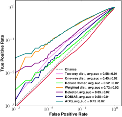
(d) 1KG, 805 SNPs, WGAN-GP

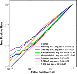
(e) 1KG, 5k SNPs, WGAN-GP

(f) 1KG, 10k SNPs, WGAN-GP

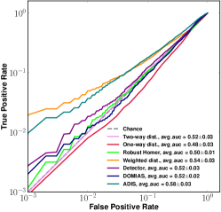
(g) dbGaP, 805 SNPs.,Vanilla

(h) dbGaP, 5k SNPs.,Vanilla

(i) dbGaP, 10k SNPs.,Vanilla

(j) dbGaP, 805 SNPs.,WGAN-GP

(k) dbGaP, 5k SNPs.,WGAN-GP

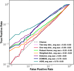
(l) dbGaP, 10k SNPs.,WGAN-GP

Figure 2: log-log ROC Curves for Vanilla GAN and WGAN-GP trained on 1KG and dbGaP.

Inspecting the results on 1KG in Figure  2, we see that when the target GAN is the Vanilla GAN, at $805$ SNPs the two-way distance attack achieves both the highest TPRs at low FPRs, and the highest AUC overall at $.66$, with all the attacks except the one-way distance attack outperforming the random baseline (curves above the diagonal) by a significant margin. As the number of SNPs increases to $5K$ and then $10K$, we see that the two-way distance attack performs worse than ADIS and the Detector, even performing worse than random guessing at $10K$. As the number of SNPs increases, the relative performance of the Robust Homer Attack increases, which we also observe in the WGAN-GP results, and on the dbGaP dataset. When the target GAN is a WGAN-GP, detector-based attacks outperform distance-based attacks or DOMIAS at every SNP dimension, which we also observe for the dbGaP dataset. While the trends in terms of relative performance of different attack methods are consistent across datasets, the actual levels of privacy leakage differ. Inspecting the dbGaP results in Figure  2f we see lower AUCs across the board, although we still observe high TPRs at low FPRs.

More generally, while the AUC results for the attack methods indicate moderately low privacy leakage relative to white-box attacks against the discriminator [17, 16, 34] or those reported against diffusion models [18], for the more meaningful metric of FPR at low fixed TPRs [27], Table 3 shows that for fixed FPRs ADIS in particular achieves TPRs that are as much as $10$x the random baseline (FPR = TPR). ADIS works especially well against WGAN-GP trained on dbGaP, with improved attack success for larger dimension.

In summary, while distance-based attacks are occassionally competitive with the detector-based attacks, the Detectors have more robust attack performance as we vary the data dimension, target GAN architecture, and dataset. While these factors impact the overall privacy leakage, they have little effect on the relative ordering of the attacks. While overall AUC is low, when we consider TPR at a fixed FPR, ADIS achieves attack results that are in some cases an order of magnitude better than the random baseline, evidence of serious privacy leakage. Moreover, the fact that ADIS consistently outperforms the Detector means that augmenting the feature space with distance-based features improved attack success relative to using the input point alone. This could be due to the fact that given our relatively small datasets, starting from the distance-based metrics enabled the algorithm to learn features more efficiently.

6 Attacks on Image GANs

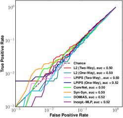
(a) Progressive GAN, CIFAR-10

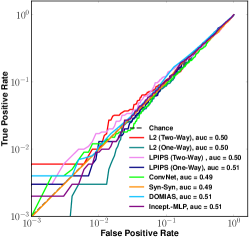
(b) ContraGAN, CIFAR-10

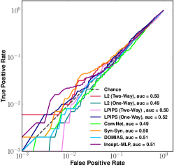
(c) BigGAN, CIFAR-10

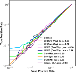
(d) DCGAN, CIFAR-10

Figure 3: log-log ROC curves for detector-based MIAs against different GAN architectures trained on CIFAR-10. While the AUCs are lower than the genomic settings, the different variants of the detector-based attacks work very well at low FPRs.

In this Section, we evaluate our attacks against $4$ GAN architectures trained on images from the CIFAR-10 dataset. We observe that relative to high dimensional tabular datasets, image GANs exhibit less privacy leakage on average, with AUCs that are barely above the random baseline. However, for the most meaningful metric, TPR at low FPRs, our detector-based attacks, and in some cases the distance-based attacks, are again able to achieve TPRs that are $2-6\times$ higher than the random baseline.

6.1 Experimental Details

We focused on GANs trained on the CIFAR-10 image dataset [20]. CIFAR-10 consists of $60000$ images across $10$ object categories, and so when sub-sampling the dataset for training the target GAN, Detectors, and evaluation, we performed stratified sampling to ensure balance across categories. The test sample size was set to $2000$ such that we have $200$ objects from each category, with $50000$ images used to train the target GAN, and $9000$ used to train the Detectors.

Four state-of-the-art GAN variants were trained: large-scale GANs for high fidelity image synthesis  [39], Conditional GANs with Projective Discriminator (PDGAN)  [56], Deep Convolutional Generative Adversarial Networks (DCGAN)  [41], and Contrastive Learning for Conditional Image Synthesis  [40]. We trained the GANs using the implementations in the Pytorch StudioGAN library [57].

We observed that training the Detector on image data proved a more delicate process than distinguishing genomic data – as a result we implemented $3$ Detector architectures. The first variant trains a CNN-based Detector  [58, 59]. In the second variant we extracted features from the training images using a pre-trained model (Inception model architecture)  [60] and fed this to an MLP pipeline. In the final variant, we trained a variational auto-encoder (VAE)  [61] on the $9000$ reference data images, and then trained a CNN classifier  [58] on synthetic samples from the VAE (label $0$) and synthetic samples from the target GAN (label $1$). This idea of training a second generative model on the reference data was proposed in [17]. Further details on Detector architectures, training parameters, and convergence plots are deferred to Section C.1 in the Appendix.

6.2 MIA Attack Success

Recall that for the image GANs we have $3$ variants of the detector attack, DOMIAS, and two distance measures ($\ell_{2}$, LPIPS [62]) were utilized for the distance-based attack. Each distance measure contributes $2$ attack types: one-way and two-way, and so for the full results in the Appendix we have a total of $8$ attacks. We summarize the results in Figure 3 and Table 3 We see that at low FPRs $<10^{-2}$, the Detector that achieves the highest TPR varies based on the target GAN architecture. For all of the target GANs Incept-MLP has the highest AUC of the detector-based methods, but performs poorly at low FPRs, albeit on BigGAN, where its AUC is about the same as the other methods. DOMIAS performs better on a relative basis on the image GANs, with the best performance in terms of AUC and low FPRs on DCGAN and second best performance at low FPRs on ContraGAN. However, when the target GAN was Progressive GAN or BigGAn, DOMIAS performed worse than random guessing at low FPRs, and so its performance overall seems inconsistent. This is an interesting direction for future investigation.

7 Conclusion

Our work provides the most thorough existing empirical analysis of attacks against GANs in the black-box setting. We prove theoretical results that build intuition for why a network that can detect samples generated from the GAN can also detect samples from the training set (Theorem 4.1), a result that has applications across all privacy attacks on ML models, not just GANs, and conduct an extremely thorough empirical evaluation of detector-based attacks, comparing their performance to existing black-box attacks across tabular and image domains. This work also raises several interesting directions for future research: although we expose significant privacy leakage from GANs, particularly at low FPRs, relative to other generative models explored in prior work, for example VAEs [25] or diffusion models [18], black-box access to the generator seems much more private. Is this actually the case, or is it simply a matter of developing better attack methods? If so, can we prove theoretically why GANs appear to be more privacy-preserving than other generative models?

Appendix A Lemmas and Proofs

We include the lemmas and proofs from the main paper in this section.

Lemma A.1.

$$\text{TPR}_{\mathcal{R}}(f)\leq\text{TPR}_{\mathcal{M}}(f)+\frac{\text{Lip}(f)}{2}W^{1}(\mathcal{G},\mathcal{T}),$$

Proof.

$\text{TPR}_{\mathcal{R}}(f)=\frac{1}{2}\mathbb{E}_{\mathcal{T}}[f(x)]=\frac{1}{2}(\mathbb{E}_{\mathcal{G}}[f(x)]+\mathbb{E}_{\mathcal{T}}[f(x)]-\mathbb{E}_{\mathcal{G}}[f(x)])=\text{TPR}_{\mathcal{M}}(f)+\frac{1}{2}(\mathbb{E}_{\mathcal{T}}[f(x)]-\mathbb{E}_{\mathcal{G}}[f(x)])\leq\text{TPR}_{\mathcal{M}}(f)+\frac{1}{2}|\mathbb{E}_{\mathcal{T}}[f(x)]-\mathbb{E}_{\mathcal{G}}[f(x)])|\leq\text{TPR}_{\mathcal{M}}(f)+\frac{1}{2\text{Lip}(f)}\sup_{g:\text{Lip}(g)=1}|\mathbb{E}_{\mathcal{T}}[f(x)]-\mathbb{E}_{\mathcal{G}}[f(x)])|=\text{TPR}_{\mathcal{M}}(f)+\frac{1}{2\text{Lip}(f)}W^{1}(\mathcal{G},\mathcal{T})$. ∎

Appendix B Attacks

We discuss the details of the different attack types in this section.

B.1 Robust Homer Attack

The intuition behind the attack lies in Line $7$ of Algorithm 1. Recall $X_{G}$ denotes synthetic samples from the GAN, $X_{R}$ denotes reference data sampled from $\mathcal{P}$, and $\tau\sim\mathcal{R}$ denotes a test point. Let $\mu_{g}=\frac{1}{n}\sum\limits_{i=0}^{n}x_{gi}\quad\text{where }\quad x_{g0},x_{g1},\dots x_{gn}\in X_{G}\quad\text{and}\quad\mu_{g}\in{[0,1]}^{d}$. Similarly, let $\mu_{r}=\frac{1}{m}\sum\limits_{i=\mathbf{1}}^{m}x_{i}\quad\text{where }\quad x_{1},x_{2}\dots x_{m}\in X_{R}\quad\text{and}\quad\mu_{r}\in{[0,1]}^{d}$. Then sample $x\sim\mathcal{P}$, and compute:

$$\langle\tau-x,\mu_{g}-\mu_{r}\rangle=\langle\tau,\mu_{g}-\mu_{r}\rangle-\langle x,\mu_{g}-\mu_{r}\rangle=\underbrace{\big{[}\langle\tau,\mu_{g}\rangle-\langle x,\mu_{g}\rangle\big{]}}_{(1)}+\underbrace{\big{[}\langle x,\mu_{r},\rangle-\langle\tau,\mu_{r},\rangle\big{]}}_{(2)}$$

Part $(1)$ above checks if $\tau$ is more correlated with $\mu_{g}$ than a random sample $x$ from $\mathcal{P}$, while $(2)$ checks if $x$ is more correlated with $\mu_{r}$ than $\tau$. Observe that this is similar to the intuition behind the distance-based attack, but here we compute an average similarity measure to $\mu_{g}$ and $\mu_{r}$, rather than a distance to the closest point.

Algorithm 1 Robust Homer Attack

1:$(X_{R}\in\{0,1\}^{d},G,x\sim\mathcal{R})$

2:$\mu_{r}=\frac{1}{m}\sum\limits_{i=1}^{m}x_{i}\quad\text{where }\quad x_{1},x_{2}\dots x_{m}\in X_{R}$

3:$\alpha\leftarrow\frac{1}{\sqrt{m}}+\epsilon,\quad\eta\leftarrow 2\alpha$ $\triangleright$ $\epsilon\geq 0$

4:$X_{G}\sim\mathcal{G}$ $\triangleright$ $X_{G}\in{\{0,1\}}^{d}$

5:$\mu_{g}=\frac{1}{n}\sum\limits_{i=0}^{n}x_{gi}\quad\text{where }\quad x_{g0},x_{g1},\dots x_{gn}\in X_{G}\quad\text{and}\quad\mu_{g}\in{[0,1]}^{d}$

6:Let ${\left\lfloor{\mu_{g}-\mu_{r}}\right\rceil}_{\eta}\in{[-\eta,+\eta]}^{d}$ $\triangleright$ entry-wise truncation of $\mu_{g}-\mu_{r}\,$ to $[-\eta,\eta]$

7:for  $\tau\sim\mathcal{R}$  do

8:     $\rho\leftarrow\langle\tau-x,{\left\lfloor{\mu_{g}-\mu_{r}}\right\rceil}_{\eta}\rangle$

9:     if $\rho>\kappa$ then $\triangleright$ $\kappa$ is an hyperparameter

10:         $\tau$ is in training set for $G$

11:     else

12:         $\tau$ is not in training set for $G$

13:     end if

14:end for

B.2 Distance Attacks on Image GAN

The choice of metric for the distance-based attack on image GANs requires some careful consideration. Though $\ell_{2}$ distance was suggested in  [16],  [63] notes that it can’t capture joint image statistics since it uses point-wise differences to measure image similarity  [63]. More recently, with the widespread adoption of deep neural networks, learning-based metrics have enjoyed wide popularity and acceptance  [64, 65, 66]. These metrics leverage pre-trained deep neural networks to extract features and use these features as the basis for metric computation  [63]. LPIPS  [62] (Learned Perceptual Image Patch Similarity) is the most common of such learning-based metrics and was also proposed in  [16] for carrying out distance-based attacks. Our distance-based attacks are implemented using both $\ell_{2}$ distance and LPIPS.

B.3 Detector Attack

The target GAN configurations for the genomic data setting are shown in Table  1.

Table 1: Target GAN configurations for genomic Data

Data	SNPs Dim.	Train Data Size	Ref. Data Size	Test Size	GAN Variant
1000 Genome	805	3000	2008	1000	vanilla & WGAN-GP
	5000	3000	2008	1000	vanilla & WGAN-GP
	1000	3000	2008	1000	vanilla & WGAN-GP
dbGaP	805	6500	5508	1000	vanilla & WGAN-GP
	5000	6500	5508	1000	vanilla & WGAN-GP
	10000	6500	5508	1000	vanilla & WGAN-GP

Detector Prediction Score.

In order to verify our Detectors succeed at the task for which they were trained, classifying samples from $\mathcal{M}$, in Table  2 we report the test accuracy for our Detectors.

Table 2: Detector Test Accuracy

Data	GAN Variant	SNPs Dim.	Test Size	Train Epochs	Mean Accuracy
1000 Genome	vanilla	805	1000	159	0.974
	vanilla	5000	3000	240	0.980
	vanilla	1000	3000	360	0.999
dbGaP	WGAN-GP	805	1000	300	0.995
	WGAN-GP	5000	1000	600	0.998
	WGAN-GP	10000	6500	1500	0.930

Detector Architecture for Genomic Data Setting

Figure  4 shows the Detector model architectures implemented in Keras [67] and Tensorflow [68] for the MIAs on genomic GANs. The exact architecture differs depending on the dimension of the input data.

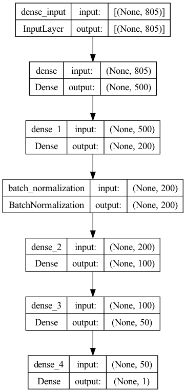
(a) Architecture for 805 SNPs

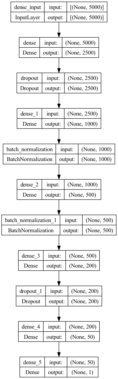
(b) Architecture for 5000 SNPs

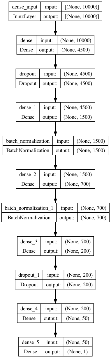
(c) Architecture for 10000 SNPs

Figure 4: Detector Architecture for MIA against Vanilla GAN trained on 1000 genome database for 805, 5000, and 10000 SNPS configurations. The Detector architecture varies depending on the SNPs configurations.

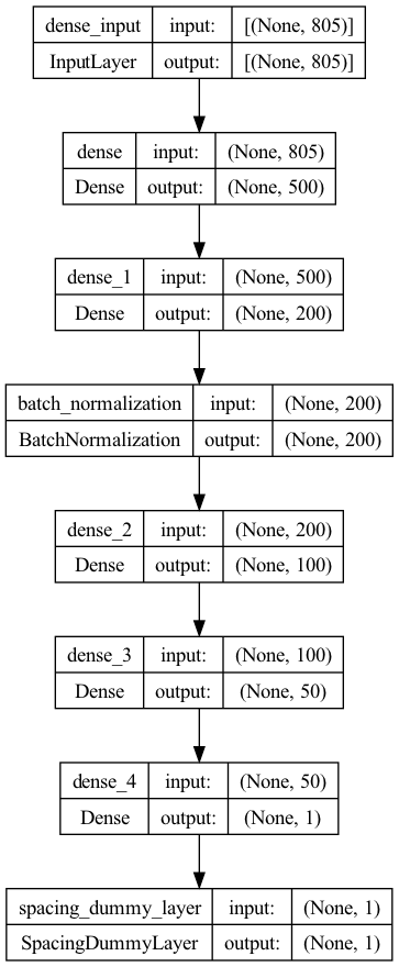
(a) Architecture for 805 SNPs

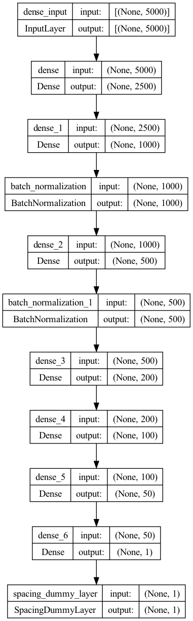
(b) Architecture for 5000 SNPs

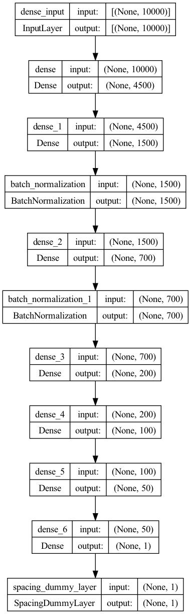
(c) Architecture for 10000 SNPs

Figure 5: Detector Architecture for MIA against Vanilla GAN trained on 1000 genome database for 805,5000 and 10000 SNP dimension. The Detector architecture varies depending on the SNPs configurations.

B.4 Augmented Detector(ADIS)

ADIS builds on the Detector by augmenting the feature space with variables derived from distance metrics and the DOMIAS attack. The pipeline is the same as that of training the Detector, with the following initial pre-processing step that creates the input to the network:

1. Sample $N(\approx 200)$ data points from $\mathcal{P},\mathcal{G}$ respectively. The sub-sampled data are for the computation of the reconstruction losses (see Section 4.2) and are not included again in the downstream training set.

2. Apply dimensionality reduction separately to synthetic and reference samples, using PCA (details below).

3. Given a test point $x\sim\mathcal{M}$, augment the feature space with test statistics computed using the projected and non-projected sample. We compute distance-based test statistics (one-way and two distances computed using the held-out sample), and the DOMIAS likelihood ratio statistic $\frac{P_{G}(x)}{P_{R}(x)}$  [26] where $P_{G}$ and $P_{X_{R}}$ are density models fitted on the synthetic and reference data respectively.

ADIS Training Details.

The architecture for ADIS is the same as the Detector, but there are additional preprocessing steps and fewer epochs ($\approx$ 10-30 epochs). A fixed sample size of $300$ from the reference and synthetic sample was set aside for the computation of reconstruction losses. This was followed by fitting principal component analysis (PCA)  [69, 70] on the training data (consisting of reference and synthetic data) and selecting the first $100\text{-}300$ principal components - the actual component selected depends on the dimension of the original feature space, but typically $100$ components were selected for 805 SNPs and $300$ for $5000$ SNPs. Subsequently, we computed one-way and two-way Hamming reconstruction losses on the non-transformed training data. Furthermore, as recommended in  [34], we computed the two-way $\ell_{2}$ reconstruction loss on the PCA-transformed training data. Note that the $300$ samples we set aside had to be PCA-transformed before being used for the computation of two-way $\ell_{2}$ reconstruction loss. For the computation of the test statistics of DOMIAS  [26], we first reduced the dimensionality of the synthetic samples and reference data separately with the fitted PCA. Then we fit a Gaussian mixture model  [71], $P_{G}$, on the PCA-transformed synthetic samples and another Gaussian mixture model, $P_{X_{R}}$, on the PCA-transformed reference data. Finally, we computed the test statistic $\frac{P_{G}(x)}{P_{X_{R}}(x)}$ for each PCA-transformed training point $x$.

Training DOMIAS

Training DOMIAS involves 2 steps – dimensionality reduction and density estimation. In the genomic data setting, we used PCA for dimension reduction following the same steps as described for ADIS. For density estimation, we using the non-volume preserving transformation (NVP)[72]. We fit the the estimator to the synthetic and reference samples separately. For image data, we projected the image onto a low dimensional sub-space using the encoder of a VAE trained on the reference and synthetic data. Subsequently, we fit the density estimator using NVP on the transformed data.

Appendix C Convergence Plots And Memorization

We present PCA convergence plots for GANs trained on genomic data and empirical analysis of memorization in these GANs.

C.1 Genomic GAN Convergence Plots

For image data, visual inspection is a quick way to examine if the synthetic samples have converged to the underlying training samples. Clearly, with high-dimensional tabular data such quick visual convergence examination does not work. Recent work [73] proposed using both the principal component analysis (PCA) and $t$-distributed stochastic neighbor embedding (T-SNE) plots for the analysis of genomic data population structure. Consequently, we examine the convergence of the synthetic samples using both PCA and T-SNE. In particular, the synthetic samples converge if the population structure as captured by the PCA and T-SNE is similar to that of the corresponding real genomic samples. Figures 6a - 6f depict the 6 principal components of both the training data and synthetic samples for each configuration in Table 1. Based on the plots it appears the synthetic samples are indeed converging towards the underlying data distribution.

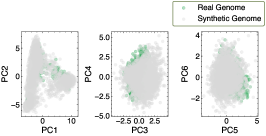
(a) 805 SNPS, 1k Genome

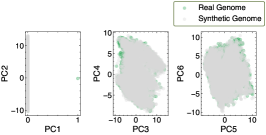
(b) $5$k SNPS, 1k Genome

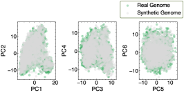
(c) 10 SNPS, 1k Genome

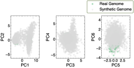
(d) 805 SNPS, dbGaP

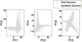
(e) $5$k SNPS, dbGaP

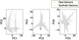
(f) $10$k SNPS, dbGaP

Figure 6: PCA Plots for all data configurations. The plot could be read row-wise or column-wise. The first row depicts PCA plots for synthetic samples from Vanilla GAN trained on 1000 Genome data for $805$, $5$k, and $10$k SNPS respectively. The second row depicts PCA plots for synthetic samples from WGAN trained on dbGaP data for $805$, $5$k, and $10$k SNPs respectively. Each column corresponds to 805,$5$k and $10$k SNPS configurations.

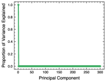
(a) $5$k SNPS, 1k Genome

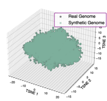
(b) $5$k SNPS, 1k Genome

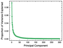
(c) $10$k SNPS, 1k Genome

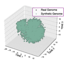
(d) $10$k SNPS, 1k Genome

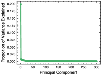
(e) $5$k SNPS, dbGaP

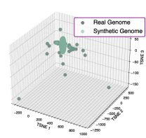
(f) $10$k SNPS,

(g) $10$k SNPS, dbGaP

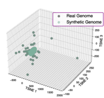
(h) $10$k SNPS, dbGaP

Figure 7: The first row shows scree and TSNE plots for synthetic samples from Vanilla GAN trained on 1000 Genome data for $5$k, $10$k SNPS respectively. The second row shows scree and TSNE plots for synthetic samples from WGAN trained on dbGaP data for $5$k, and $10$k SNPS respectively. The distance metric for the reconstruction loss is the Hamming distance.

C.2 Over-fitting and Memorization

This section performs some preliminary analyses on the genomic data GANs to ensure they aren’t memorizing the training set. Memorization is one indicator of overfitting, which would artificially inflate the attack success metrics of our MIAs.

Whole sequence memorization.

We iteratively sample batches of $3000$-$4000$ synthetic samples, $S_{B}$, from the GAN until the sample size is of order $\geq 10^{6}$. For each sample point in the $i$-th batch, $s_{b}\in S_{B_{i}}$ , we compute its minimum Hamming distance to $\mathcal{P}$, the training data. Observe that a Hamming distance of zero would indicate whole sequence memorization - since it implies that an exact copy of a training data sample is being synthesized by the GAN. Figures 8, 9 show the GAN models do not memorize the training data, since no reconstruction losses of zero are reported.

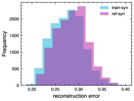
(a) 805 SNPS,1k Genome

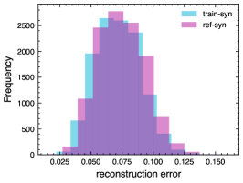
(b) $5$k SNPS,1k Genome

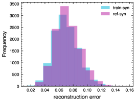
(c) $10$k SNPS,1k Genome

Figure 8: The plots show the frequency distribution of reconstruction error for whole sequence memorization test for 3 batches of synthetic samples from vanilla GAN trained. The label train-syn (in seafoam green) indicates that we are measuring reconstruction loss for each batch of the synthetic samples with respect to the training data. For reference purposes, we also plot, ref-syn, which is the reconstruction loss of the synthetic samples given the reference samples (in purple). The distance metric for the reconstruction loss is the Hamming distance.

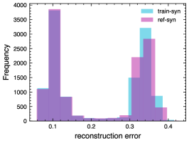
(a) 805 SNPs, dbGaP

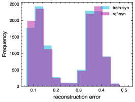
(b) $5$k SNPs, dbGap

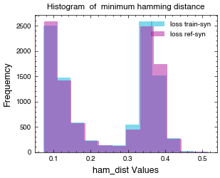
(c) $10$k SNPs, dbGaP

Figure 9: The plots show the frequency distribution of reconstruction error for 3 batches of synthetic samples from WGAN-GP. The label train-syn (in seafoam green) indicates that we are measuring reconstruction loss for each batch of the synthetic samples with respect to the training data . For reference purposes, we plot ref-syn, which is the reconstruction loss of the synthetic samples given the reference samples (in purple). The distance metric for the reconstruction loss is the Hamming distance.

Appendix D Results Table for Genomic GANs (TPR At Low FPR)

Table 3 depicts the TPR at FPR of $0.01$ , $0.1$, $0.005$ and $0.001$ respectively (see Figures 2 and 2d) for genomic data setting.

Table 3: Table of Attack Results (Genomic Data)

GAN Variant	Dataset	Attack Method	TPR @0.01 FPR	TPR @ 0.1 FPR	TPR @0.005 FPR	TPR @0.001 FPR
vanilla 805	1000 genome	one-way distance	1.02%	6.95%	0.51%	0.13%
vanilla 805	1000 genome	two-way distance	7.79%	28.86%	5.14%	1.89%
vanilla 805	1000 Genome	weighted distance	4.75%	21.76 %	2.85%	1.76%
vanilla 805	1000 Genome	Robust Homer	2.46%	17.89%	1.26%	0.20%
vanilla 805	1000 Genome	Detector	1.89%	13.72%	0.97%	0.19%
vanilla 805	1000 Genome	ADIS	5.31%	26.89%	3.14%	1.16%
vanilla $5$k	1000 genome	one-way distance	0.88%	7.6%	0.37%	0.10%
vanilla $5$k	1000 genome	two-way distance	1.36%	13.89%	0.68%	0.25%
vanilla $5$k	1000 Genome	weighted distance	1.00%	12.6%	0 .56%	0.15%
vanilla $5$k	1000 Genome	Robust Homer	0.88%	7.62%	0.58%	0.25%
vanilla $5$k	1000 Genome	Detector	1.52%	12.70%	0.82%	0.33%
vanilla $5$k	1000 Genome	ADIS	2.00%	13.40%	0.99%	0.26%
vanilla $10$k	1000 genome	one-way distance	1.10%	9.97%	0.62%	0.23%
vanilla $10$k	1000 genome	two-way distance	1.07%	10.52%	0.42%	0.17%
vanilla $10$k	1000 Genome	weighted distance	0.90%	10.4%	0.49%	0.15%
vanilla $10$k	1000 Genome	Robust Homer	1.11%	10.56%	0.58%	0.36%
vanilla $10$k	1000 Genome	Detector	1.38%	11.56%	0.68%	0.17%
vanilla $10$k	1000 Genome	ADIS	1.72%	12.56%	1.03%	0.25%
wgan-gp 805	dbGaP	one-way distance	0.91%	7.69%	0.54%	0.23%
wgan-gp 805	dbGaP	two-way distance	1.52%	11.91%	0.63%	0.23%
wgan-gp 805	dbGaP	weighted distance	1.41%	11.75%	0.91%	0.38%
wgan-gp 805	dbGaP	Robust Homer	1.37%	11.22%	0.67%	0.25%
wgan-gp 805	dbGaP	Detector	2.59%	16.01%	1.14%	0.22%
wgan-gp 805	dbGaP	ADIS	2.40%	15.15%	1.04%	0.35%
wgan-gp $5$k	dbGaP	one-way distance	0.93%	9.17%	0.23%	0.16%
wgan-gp $5$k	dbGaP	two-way distance	1.62%	12.81%	0.77%	0.29%
wgan-gp $5$k	dbGaP	weighted distance	1.90%	12.90%	1.90%	0.35%
wgan-gp $5$k	dbGaP	Robust Homer	2.13%	14.03%	1.48%	0.62%
wgan-gp $5$k	dbGaP	Detector	2.95%	20.10%	1.64%	0.37%
wgan-gp $5$k	dbGaP	ADIS	6.40%	28.70%	3.98%	1.32%
wgan-gp $10$k	dbGaP	one-way distance	1.42%	9.38%	0.55%	0.09%
wgan-gp $10$k	dbGaP	two-way distance	2.07%	12.45%	1.20%	0.47%
wgan-gp $10$k	dbGaP	weighted distance	1.96%	11.80%	0.98%	0.45%
wgan-gp $10$k	dbGaP	Robust Homer	2.71%	13.95%	1.35%	0.65%
wgan-gp $10$k	dbGaP	Detector	3.26%	24.23%	2.11%	0.67%
wgan-gp $10$k	dbGaP	ADIS	6.07%	24.49%	4.24%	1.6%

Appendix E Results Table for Image GANs (TPR At Low FPR)

Table 4 depicts the TPR at FPR of $0.01$ , $0.1$, $0.005$ and $0.001$ respectively (see Figures 2 and 2d) for genomic data setting.

Table 4: Table of Attack Results (Image Data)

GAN Variant	Dataset	Attack Method	TPR @0.01 FPR	TPR @0.1 FPR	TPR @0.005 FPR	TPR @0.001 FPR
BigGAN	CIFAR10	two-way distance ($\ell_{2}$)	1.0%	10.8%	0.6%	0.6%
BigGAN	CIFAR10	one-way distance ($\ell_{2}$)	0.6%	8.7%	0.2%	0.0%
BigGAN	CIFAR10	two-way distance (LPIPS)	0.4%	11.0%	0.1%	0.1%
BigGAN	CIFAR10	one-way distance (LPIPS)	1.2%	10.8%	0.7%	0.1%
BigGAN	CIFAR10	Detector (Conv. net)	0.8%	7.7%	0.3%	0.0%
BigGAN	CIFAR10	Detector (syn-syn)	1.4%	11.8%	0.7%	0.2%
BigGAN	CIFAR10	Detector(Incept.-MLP)	2.2%	9.3%	1.6%	0.2%
DCGAN	CIFAR10	two-way distance ($\ell_{2}$)	1.0%	10.8%	0.6%	0.6%
DCGAN	CIFAR10	one-way distance ($\ell_{2}$)	1.0%	11.1%	0.6%	0.6%
DCGAN	CIFAR10	two-way distance (LPIPS)	1.2%	13.0%	0.7%	0.3%
DCGAN	CIFAR10	one-way distance (LPIPS)	1.7%	9.0%	0.6%	0.2%
DCGAN	CIFAR10	Detector (Conv. net)	1.4%	9.7%	1.1%	0.3%
DCGAN	CIFAR10	Detector (syn-syn)	1.2%	9.6%	0.6%	0.1%
DCGAN	CIFAR10	Detector (Incept.-MLP)	0.8%	11.4%	0.4%	0.2%
ProjGAN	CIFAR10	two-way distance ($\ell_{2}$)	1.0%	10.7%	0.6%	0.6%
ProjGAN	CIFAR10	one-way distance ($\ell_{2}$)	0.6%	8.4%	0.3%	0.1%
ProjGAN	CIFAR10	two-way distance (LPIPS)	0.7%	10.7%	0.6%	0.1%
ProjGAN	CIFAR10	one-way distance (LPIPS)	1.0%	10.9%	0.8%	0.6%
ProjGAN	CIFAR10	Detector (Conv. net)	1.5%	9.9%	0.7%	0.1%
ProjGAN	CIFAR10	Detector (syn-syn)	2.0%	11.8%	1.4%	0.1%
ProjGAN	CIFAR10	Detector (Incept.-MLP)	0.9%	11.6%	0.2%	0.0%
ContraGAN	CIFAR10	two-way distance ($\ell_{2}$)	1.0%	10.8%	0.6%	0.6%
ContraGAN	CIFAR10	one-way distance ($\ell_{2}$)	0.3%	8.7%	0.3%	0.0%
ContraGAN	CIFAR10	two-way distance (LPIPS)	1.7%	12.3%	1.0%	0.3%
ContraGAN	CIFAR10	one-way distance (LPIPS)	1.3%	10.4%	0.4%	0.3%
ContraGAN	CIFAR10	Detector (Conv. net)	1.2%	9.6%	0.7%	0.1%
ContraGAN	CIFAR10	Detector (syn-syn)	0.9%	10.0%	0.5%	0.01%
ContraGAN	CIFAR10	Detector (Incept.-MLP)	0.9%	10.4%	0.3%	0.2%

References

- [1] Ian J. Goodfellow, Jean Pouget-Abadie, Mehdi Mirza, Bing Xu, David Warde-Farley, Sherjil Ozair, Aaron Courville, and Yoshua Bengio. Generative adversarial networks, 2014.
- [2] Jascha Sohl-Dickstein, Eric A. Weiss, Niru Maheswaranathan, and Surya Ganguli. Deep unsupervised learning using nonequilibrium thermodynamics. CoRR, abs/1503.03585, 2015.
- [3] Jonathan Ho, Ajay Jain, and Pieter Abbeel. Denoising diffusion probabilistic models. CoRR, abs/2006.11239, 2020.
- [4] Zhifeng Kong, Wei Ping, Jiaji Huang, Kexin Zhao, and Bryan Catanzaro. Diffwave: A versatile diffusion model for audio synthesis, 2020.
- [5] Jonathan Ho, Tim Salimans, Alexey Gritsenko, William Chan, Mohammad Norouzi, and David J. Fleet. Video diffusion models, 2022.
- [6] Lei Wang, Wei Chen, Wenjia Yang, Fangming Bi, and Fei Richard Yu. A state-of-the-art review on image synthesis with generative adversarial networks. IEEE Access, 8:63514–63537, 2020.
- [7] Jungil Kong, Jaehyeon Kim, and Jaekyoung Bae. Hifi-gan: Generative adversarial networks for efficient and high fidelity speech synthesis. Advances in Neural Information Processing Systems, 33:17022–17033, 2020.
- [8] Ming-Yu Liu, Xun Huang, Jiahui Yu, Ting-Chun Wang, and Arun Mallya. Generative adversarial networks for image and video synthesis: Algorithms and applications. Proceedings of the IEEE, 109(5):839–862, 2021.
- [9] Ting-Chun Wang, Ming-Yu Liu, Jun-Yan Zhu, Guilin Liu, Andrew Tao, Jan Kautz, and Bryan Catanzaro. Video-to-video synthesis. CoRR, abs/1808.06601, 2018.
- [10] Lei Xu, Maria Skoularidou, Alfredo Cuesta-Infante, and Kalyan Veeramachaneni. Modeling tabular data using conditional gan. Advances in Neural Information Processing Systems, 32, 2019.
- [11] Zilong Zhao, Aditya Kunar, Robert Birke, and Lydia Y. Chen. Ctab-gan: Effective table data synthesizing. In Vineeth N. Balasubramanian and Ivor Tsang, editors, Proceedings of The 13th Asian Conference on Machine Learning, volume 157 of Proceedings of Machine Learning Research, pages 97–112. PMLR, 17–19 Nov 2021.
- [12] Minguk Kang, Jun-Yan Zhu, Richard Zhang, Jaesik Park, Eli Shechtman, Sylvain Paris, and Taesung Park. Scaling up gans for text-to-image synthesis. In Proceedings of the IEEE Conference on Computer Vision and Pattern Recognition (CVPR), 2023.
- [13] Tero Karras, Miika Aittala, Samuli Laine, Erik Härkönen, Janne Hellsten, Jaakko Lehtinen, and Timo Aila. Alias-free generative adversarial networks. In Proc. NeurIPS, 2021.
- [14] Katherine Crowson, Stella Biderman, Daniel Kornis, Dashiell Stander, Eric Hallahan, Louis Castricato, and Edward Raff. Vqgan-clip: Open domain image generation and editing with natural language guidance. In European Conference on Computer Vision, pages 88–105. Springer, 2022.
- [15] Drew A. Hudson and C. Lawrence Zitnick. Generative adversarial transformers. CoRR, abs/2103.01209, 2021.
- [16] Dingfan Chen, Ning Yu, Yang Zhang, and Mario Fritz. GAN-Leaks: A Taxonomy of Membership Inference Attacks against Generative Models. In Proceedings of the 2020 ACM SIGSAC Conference on Computer and Communications Security, pages 343–362, October 2020. arXiv:1909.03935 [cs].
- [17] Jamie Hayes, Luca Melis, George Danezis, and Emiliano De Cristofaro. Logan: Membership inference attacks against generative models, 2018.
- [18] Nicholas Carlini, Jamie Hayes, Milad Nasr, Matthew Jagielski, Vikash Sehwag, Florian Tramèr, Borja Balle, Daphne Ippolito, and Eric Wallace. Extracting training data from diffusion models, 2023.
- [19] Boris van Breugel, Hao Sun, Zhaozhi Qian, and Mihaela van der Schaar. Membership inference attacks against synthetic data through overfitting detection, 2023.
- [20] Alex Krizhevsky. Learning multiple layers of features from tiny images. 2009.
- [21] Ian C Gray, David A Campbell, and Nigel K Spurr. Single nucleotide polymorphisms as tools in human genetics. Human molecular genetics, 9(16):2403–2408, 2000.
- [22] Kimberly A Tryka, Luning Hao, Anne Sturcke, Yumi Jin, Zhen Y Wang, Lora Ziyabari, Moira Lee, Natalia Popova, Nataliya Sharopova, Masato Kimura, et al. Ncbi’s database of genotypes and phenotypes: dbgap. Nucleic acids research, 42(D1):D975–D979, 2014.
- [23] 1000 Genomes Project Consortium et al. A global reference for human genetic variation. Nature, 526(7571):68, 2015.
- [24] Nils Homer, Szabolcs Szelinger, Margot Redman, David Duggan, John Tembe, Jill Muehling, John V. Pearson, Dietrich A. Stephan, Stanley F. Nelson, and David W. Craig. Resolving individuals contributing trace amounts of DNA to highly complex mixtures using high-density SNP genotyping microarrays. PLoS Genetics, 4(8):e1000167, August 2008.
- [25] J Hayes, L Melis, G Danezis, and E De Cristofaro. Logan: Membership inference attacks against generative models. In Proceedings on Privacy Enhancing Technologies (PoPETs), volume 2019, pages 133–152. De Gruyter, 2019.
- [26] Boris van Breugel, Hao Sun, Zhaozhi Qian, and Mihaela van der Schaar. Membership inference attacks against synthetic data through overfitting detection, 2023.
- [27] Nicholas Carlini, Steve Chien, Milad Nasr, Shuang Song, Andreas Terzis, and Florian Tramèr. Membership inference attacks from first principles. CoRR, abs/2112.03570, 2021.
- [28] Reza Shokri, Marco Stronati, Congzheng Song, and Vitaly Shmatikov. Membership Inference Attacks against Machine Learning Models, March 2017. arXiv:1610.05820 [cs, stat].
- [29] Samuel Yeom, Irene Giacomelli, Matt Fredrikson, and Somesh Jha. Privacy Risk in Machine Learning: Analyzing the Connection to Overfitting. In 2018 IEEE 31st Computer Security Foundations Symposium (CSF), pages 268–282, July 2018. ISSN: 2374-8303.
- [30] Milad Nasr, Reza Shokri, and Amir Houmansadr. Comprehensive privacy analysis of deep learning: Passive and active white-box inference attacks against centralized and federated learning. In 2019 IEEE Symposium on Security and Privacy (SP). IEEE, may 2019.
- [31] Gilad Cohen and Raja Giryes. Membership inference attack using self influence functions, 2022.
- [32] Martin Pawelczyk, Himabindu Lakkaraju, and Seth Neel. On the privacy risks of algorithmic recourse, 2022.
- [33] Christopher A. Choquette-Choo, Florian Tramèr, Nicholas Carlini, and Nicolas Papernot. Label-only membership inference attacks. CoRR, abs/2007.14321, 2020.
- [34] Benjamin Hilprecht, Martin Härterich, and Daniel Bernau. Monte carlo and reconstruction membership inference attacks against generative models. Proc. Priv. Enhancing Technol., 2019(4):232–249, 2019.
- [35] Burak Yelmen, Aurélien Decelle, Linda Ongaro, Davide Marnetto, Corentin Tallec, Francesco Montinaro, Cyril Furtlehner, Luca Pagani, and Flora Jay. Creating artificial human genomes using generative neural networks. PLOS Genetics, 17(2):e1009303, February 2021.
- [36] Andrew Yale, Saloni Dash, Ritik Dutta, Isabelle Guyon, Adrien Pavao, and Kristin P. Bennett. Privacy Preserving Synthetic Health Data. April 2019.
- [37] Martin Arjovsky, Soumith Chintala, and Léon Bottou. Wasserstein Generative Adversarial Networks. In Proceedings of the 34th International Conference on Machine Learning, pages 214–223. PMLR, July 2017. ISSN: 2640-3498.
- [38] Ning Yu, Ke Li, Peng Zhou, Jitendra Malik, Larry Davis, and Mario Fritz. Inclusive GAN: Improving Data and Minority Coverage in Generative Models. In Andrea Vedaldi, Horst Bischof, Thomas Brox, and Jan-Michael Frahm, editors, Computer Vision – ECCV 2020, Lecture Notes in Computer Science, pages 377–393, Cham, 2020. Springer International Publishing.
- [39] Andrew Brock, Jeff Donahue, and Karen Simonyan. Large scale GAN training for high fidelity natural image synthesis. CoRR, abs/1809.11096, 2018.
- [40] Minguk Kang and Jaesik Park. Contragan: Contrastive learning for conditional image generation, 2021.
- [41] Alec Radford, Luke Metz, and Soumith Chintala. Unsupervised representation learning with deep convolutional generative adversarial networks, 2016.
- [42] Ian Goodfellow, Jean Pouget-Abadie, Mehdi Mirza, Bing Xu, David Warde-Farley, Sherjil Ozair, Aaron Courville, and Yoshua Bengio. Generative adversarial networks. Communications of the ACM, 63(11):139–144, October 2020.
- [43] Jinyuan Jia, Ahmed Salem, Michael Backes, Yang Zhang, and Neil Zhenqiang Gong. Memguard: Defending against black-box membership inference attacks via adversarial examples. CoRR, abs/1909.10594, 2019.
- [44] Alexandre Sablayrolles, Matthijs Douze, Yann Ollivier, Cordelia Schmid, and Hervé Jégou. White-box vs black-box: Bayes optimal strategies for membership inference, 2019.
- [45] Jiayuan Ye, Aadyaa Maddi, Sasi Kumar Murakonda, Vincent Bindschaedler, and Reza Shokri. Enhanced membership inference attacks against machine learning models. arXiv preprint arXiv:2111.09679, 2021.
- [46] Yiyong Liu, Zhengyu Zhao, Michael Backes, and Yang Zhang. Membership inference attacks by exploiting loss trajectory, 2022.
- [47] Jerzy Neyman and Egon Sharpe Pearson. Ix. on the problem of the most efficient tests of statistical hypotheses. Philosophical Transactions of the Royal Society of London. Series A, Containing Papers of a Mathematical or Physical Character, 231(694-706):289–337, 1933.
- [48] Yi Lin. A note on margin-based loss functions in classification. Statistics & Probability Letters, 68(1):73–82, 2004.
- [49] Hoang Thanh-Tung, Truyen Tran, and Svetha Venkatesh. On catastrophic forgetting and mode collapse in generative adversarial networks. CoRR, abs/1807.04015, 2018.
- [50] Nils Homer, Szabolcs Szelinger, Margot Redman, David Duggan, Waibhav Tembe, Jill Muehling, John V. Pearson, Dietrich A. Stephan, Stanley F. Nelson, and David W. Craig. Resolving Individuals Contributing Trace Amounts of DNA to Highly Complex Mixtures Using High-Density SNP Genotyping Microarrays. PLoS Genetics, 4(8):e1000167, August 2008.
- [51] Cynthia Dwork, Adam Smith, Thomas Steinke, Jonathan Ullman, and Salil Vadhan. Robust traceability from trace amounts. In 2015 IEEE 56th Annual Symposium on Foundations of Computer Science, pages 650–669, 2015.
- [52] Matthew D Mailman, Michael Feolo, Yumi Jin, Masato Kimura, Kimberly Tryka, Rinat Bagoutdinov, Luning Hao, Anne Kiang, Justin Paschall, Lon Phan, et al. The ncbi dbgap database of genotypes and phenotypes. Nature genetics, 39(10):1181–1186, 2007.
- [53] Petr Danecek, Adam Auton, Goncalo Abecasis, Cornelis A. Albers, Eric Banks, Mark A. DePristo, Robert E. Handsaker, Gerton Lunter, Gabor T. Marth, Stephen T. Sherry, Gilean McVean, Richard Durbin, and 1000 Genomes Project Analysis Group. The variant call format and VCFtools. Bioinformatics, 27(15):2156–2158, 06 2011.
- [54] Shaun Purcell, Benjamin Neale, Kathe Todd-Brown, Lori Thomas, Manuel AR Ferreira, David Bender, Julian Maller, Pamela Sklar, Paul IW De Bakker, Mark J Daly, et al. Plink: a tool set for whole-genome association and population-based linkage analyses. The American journal of human genetics, 81(3):559–575, 2007.
- [55] Ishaan Gulrajani, Faruk Ahmed, Martin Arjovsky, Vincent Dumoulin, and Aaron C Courville. Improved Training of Wasserstein GANs. In Advances in Neural Information Processing Systems, volume 30. Curran Associates, Inc., 2017.
- [56] Takeru Miyato and Masanori Koyama. cgans with projection discriminator. CoRR, abs/1802.05637, 2018.
- [57] MinGuk Kang, Joonghyuk Shin, and Jaesik Park. StudioGAN: A Taxonomy and Benchmark of GANs for Image Synthesis. IEEE Transactions on Pattern Analysis and Machine Intelligence (TPAMI), 2023.
- [58] Alex Krizhevsky, Ilya Sutskever, and Geoffrey E Hinton. Imagenet classification with deep convolutional neural networks. Communications of the ACM, 60(6):84–90, 2017.
- [59] Saad Albawi, Tareq Abed Mohammed, and Saad Al-Zawi. Understanding of a convolutional neural network. In 2017 international conference on engineering and technology (ICET), pages 1–6. Ieee, 2017.
- [60] Christian Szegedy, Wei Liu, Yangqing Jia, Pierre Sermanet, Scott Reed, Dragomir Anguelov, Dumitru Erhan, Vincent Vanhoucke, and Andrew Rabinovich. Going deeper with convolutions (2014). arXiv preprint arXiv:1409.4842, 10, 2014.
- [61] Diederik P Kingma and Max Welling. Auto-encoding variational bayes, 2022.
- [62] Richard Zhang, Phillip Isola, Alexei A. Efros, Eli Shechtman, and Oliver Wang. The unreasonable effectiveness of deep features as a perceptual metric. CoRR, abs/1801.03924, 2018.
- [63] Stephanie Fu*, Netanel Tamir*, Shobhita Sundaram*, Lucy Chai, Richard Zhang, Tali Dekel, and Phillip Isola. Dreamsim: Learning new dimensions of human visual similarity using synthetic data. arXiv:2306.09344, 2023.
- [64] Alexey Dosovitskiy and Thomas Brox. Generating images with perceptual similarity metrics based on deep networks, 2016.
- [65] Leon A. Gatys, Alexander S. Ecker, and Matthias Bethge. A neural algorithm of artistic style, 2015.
- [66] Justin Johnson, Alexandre Alahi, and Li Fei-Fei. Perceptual losses for real-time style transfer and super-resolution, 2016.
- [67] François Chollet et al. Keras. https://keras.io, 2015.
- [68] Martín Abadi, Ashish Agarwal, Paul Barham, Eugene Brevdo, Zhifeng Chen, Craig Citro, Greg S. Corrado, Andy Davis, Jeffrey Dean, Matthieu Devin, Sanjay Ghemawat, Ian Goodfellow, Andrew Harp, Geoffrey Irving, Michael Isard, Yangqing Jia, Rafal Jozefowicz, Lukasz Kaiser, Manjunath Kudlur, Josh Levenberg, Dandelion Mané, Rajat Monga, Sherry Moore, Derek Murray, Chris Olah, Mike Schuster, Jonathon Shlens, Benoit Steiner, Ilya Sutskever, Kunal Talwar, Paul Tucker, Vincent Vanhoucke, Vijay Vasudevan, Fernanda Viégas, Oriol Vinyals, Pete Warden, Martin Wattenberg, Martin Wicke, Yuan Yu, and Xiaoqiang Zheng. TensorFlow: Large-scale machine learning on heterogeneous systems, 2015. Software available from tensorflow.org.
- [69] Rasmus Bro and Age K Smilde. Principal component analysis. Analytical methods, 6(9):2812–2831, 2014.
- [70] Markus Ringnér. What is principal component analysis? Nature biotechnology, 26(3):303–304, 2008.
- [71] Douglas A Reynolds et al. Gaussian mixture models. Encyclopedia of biometrics, 741(659-663), 2009.
- [72] Laurent Dinh, Jascha Sohl-Dickstein, and Samy Bengio. Density estimation using real NVP. CoRR, abs/1605.08803, 2016.
- [73] Alexander Platzer. Visualization of snps with t-sne. PloS one, 8(2):e56883, 2013.