A long-range contact process in a random environment

Abstract

We study survival and extinction of a long-range infection process on a diluted one-dimensional lattice in discrete time. The infection can spread to distant vertices according to a Pareto distribution, however spreading is also prohibited at random times. We prove a phase transition in the recovery parameter via block arguments. This contributes to a line of research on directed percolation with long-range correlations in nonstabilizing random environments.

Introduction

The contact process is a classical model for the spread of an infection through a spatially distributed population, where individuals may spontaneously lose the infection and become susceptible again. First introduced in [Har74], the model and its multiple generalisations still attract a tremendous amount of interest coming from a great variety of fields, see e.g., [RV22, Fon+23, LS23] for rather recent contributions and, important in view of this manuscript, [Hil+22, GL22, SS23], where random environments are considered. Focussing on the discrete-time version on lattices, the contact process is equivalent to certain models in oriented percolation. In particular, the key question of survival and extinction of the infection in the contact process is in one-to-one correspondence to the existence and absence of an infinite directed path in the associated percolation model.

The arguably simplest nontrivial undirected percolation model is the $\mathbb{Z}^{2}$-lattice with either vertices or edges being open with some probability $p$ independently from each other. The models are then called site (respectively bond) percolation models and the modeling idea is usually that of water flowing through open connected components, i.e., cluster. Now the standard question is whether water can flow all the way through, i.e., whether the origin lies in an infinite cluster with positive probability. If so, we are in the socalled supercritical percolation phase and in the subcritical phase otherwise. In the particular example just mentioned, the percolation phase transition for the bond model happens at $p_{c}=1/2$ [Kes80].

However, water can only flow in the direction of gravity, so it is natural to consider directed edges. A simple directed model is the north-east model on $\mathbb{Z}^{2}$ where connections only form in the north and east direction introduced in [BH57]. As pointed out in [Dur84], the directed models may have to be handled quite differently compared to their undirected counterparts. While results are often similar, the proofs differ greatly.

As mentioned before, we want to consider contact processes, i.e., infections in space-time rather than the flow of water under gravity. As seen in the past pandemic, a multitude of different factors influence this evolution. We want to focus on the following three aspects: range of infection, sparse environments and lockdowns. More precisely, in our model we assume that the infection can spread to distant vertices with polynomial decay in the probability. Additionally, we permanently remove lattice points via iid Bernoulli random variables, thereby diluting the lattice. Similarly but now on the time axis, we independently mark time points at which the transmission of the infection to other vertices is prohibited. Based on this random environment, we build our directed bond-site percolation model.

Let us mention that spatial stretches have already been considered in [BDS91]. There, a vertex $(t,x)$ is only open with probability $p(x)\in\{p_{\mathrm{bad}},p_{\mathrm{good}}\}$ where $p(x)$ does not depend on time. It is shown that survival occurs if $p_{\mathrm{good}}$ occurs sufficiently often and $p_{\mathrm{good}}$ is sufficiently large. On the other hand, in [KSV22], the case of temporal stretches (on the bonds) has been studied. Here, survival holds even for any $p_{\mathrm{good}}>p_{c}$ given that $p_{\mathrm{good}}$ occurs sufficiently often, where $p_{c}$ is the critical parameter for directed bond percolation. The strategy behind both results is to consider environment groupings and employ a multiscale analysis, i.e., $\mathbb{Z}^{2}$ is grouped into boxes at different levels and boxes are combined to form boxes on higher levels. We will follow this general idea as well and base our construction on [Hof05] – which we have already used in [JJV23] and further extend in this paper – where percolation of the randomly stretched (undirected) lattice on $\mathbb{Z}^{2}$ has been proven. Let us note that this result has recently been refined in [LSV23] all the way to the critical parameter $p_{\mathrm{good}}>p_{c}=1/2$.

Simultanously considering temporal and spatial stretches has its own challenges. For example in [Hil+23], the authors were able to link the existence of a nontrivial phase transition on the (undirected) $\mathbb{Z}^{2}$-lattice to the moments of the stretches. As mentioned there, their current method only works with one-dimensional stretches. The problem in our setting is that spreading in space takes time – time which might not be available due to lockdowns. We alleviate this issue by allowing long-range infections. Let us note that considering a discrete-time process is not a restriction as a simple discretisation scheme yields also the continuous time case.

The paper is organised as follows:

• In Section 1, we introduce the model as well as the main result, that is, the phase transition of survival and extinction. We also give the general idea of the proof in Section 1.3.

• Section 2 introduces the core definitions and lemmas which allow us to prove the main theorem. Details and their proofs are given in Section 3 and 4.

• Section 3 deals solely with the environment grouping framework while Section 4 applies said framework. In particular, this section deals with so called “drilling” (Section 4.5) for the multiscale-renormalisation argument.

1 A long-range contact process (LoRaC)

The model is given as a bond-site percolation model. We consider a very long street $\mathbb{Z}$ where each $x\in\mathbb{Z}$ represents a location. Normally, $x$ contains a house with residents (probability $1-q^{(x)}$), i.e., a potential host for infections. On the other hand, $x$ might also just be empty (with probability $q^{(x)}$). Now, assume that there is an infection starting in house $y$. During the day, the infection might spread to other houses due to people travelling to other houses. While trips to far-away destinations are rare, they still happen considerably often via e.g. airplanes (probability $(1+|y-x|)^{-\alpha}$). Each night, all residents of a house recover with probability $1-p$. In this setting, the survival of an infection corresponds to a bond-site percolation problem on $\mathbb{Z}\times\mathbb{Z}$ (with vertices $(t,x)$).

During the pandemic, governments have enforced lockdowns during which people cannot leave their houses. Therefore, no new infections occur in that time. We mimick this in our model also: Each morning, a global lockdown is imposed with probability $q^{(t)}$. An illustration of the model is given in Figure 1.

Figure 1: We start with an infection in the origin which starts infecting other houses – preferably close ones. Lockdowns happen at $t=4$ and $5$, so no spreading occurs during this time. Infections still recover at any time with probability $1-p$. Note that, here and elsewhere, we always assume time to flow from top to bottom.

1.1 Constructing the LoRaC model

After this verbal discription, let us now give a proper definition of our model. We highlight that, as mentioned already in the introduction, contact processes are closely linked to certain directed percolation problems where the directionality reflects the passing of time.

Definition 1 (The LoRaC).

Let $q^{(t)},q^{(x)},p\in(0,1)$ as well as $\alpha>1$ be given. We consider sequences of iid Bernoulli random variables $(\mathds{T}_{t})_{t\in\mathbb{Z}}$ and $(\mathbb{X}_{x})_{x\in\mathbb{Z}}$ with parameters $q^{(t)}$ respectively $q^{(x)}$. We call $t$ good if $\mathds{T}_{t}=1$ and bad otherwise. Analogously, we call $x$ good if $\mathbb{X}_{x}=1$.

Consider the graph $G=(\mathbb{Z}\times\mathbb{Z},E)$ where $E$ consists of directed edges of the form $(t,x)\to(t+1,y)$ with $t,x,y\in\mathbb{Z}$. We study a mixed bond-site-percolation model on $G$ where all vertices and edges are open (respectively closed) independently from each other with probability

$$\mathbb{P}\{(t,x)\text{ is open}\,|\,x\text{ is good}\}=p\qquad\text{and}\qquad\mathbb{P}\{(t,x)\text{ is open}\,|\,x\text{ is bad}\}=0\,,$$

and for an edge $e=\big{(}(t,x)\to(t+1,y)\big{)}$

$$\mathbb{P}\{e\text{ is open}\,|\,t\text{ is good}\}=(1+|y-x|)^{-\alpha}\qquad\text{and}\qquad\mathbb{P}\{e\text{ is open}\,|\,t\text{ is bad}\}=\delta_{xy}$$

where $\delta_{xy}=1$ iff $x=y$ and $0$ otherwise. We call the model LoRaC for long-range contact process.

Definition 2 (Percolation).

We say that the model percolates if there exists an infinite sequence of open vertices and edges such that

$$(t_{0},x_{0})\to(t_{0}+1,x_{1})\to(t_{0}+2,x_{2})\to\dots$$

almost surely. In this setting, an infection starting in $x_{0}$ at time $t_{0}$ will spread through open edges and vertices and therefore survive forever.

If $\alpha\leq 1$, then each vertex has infinitely many outgoing edges and therefore we already have an infinite number of infected houses in the first step as well as all subsequent steps. Therefore this case is trivial. If $\alpha>1$ however, the infection may die out in certain regimes.

Proposition 3 (Extinction).

1. Let $q^{(t)},q^{(x)}\in(0,1)$ and $\alpha>1$ be given. Then, there exists $p_{c}\in(0,1)$ such that for every $p<p_{c}$, the model does not percolate.

2. Let $q^{(t)},q^{(x)},p\in(0,1)$ be given. Then, there exists $\alpha_{c}>1$ such that for every $\alpha>\alpha_{c}$, the model does not percolate.

Proof.

Point 1 and 2 follow from a simple branching process argument. In these cases, we completely ignore the environment since it benefits extinction. $\alpha>1$ implies that the number of potential offsprings has expectation at most $2\zeta(\alpha)-1$ where

$$\zeta(\alpha):=\sum_{k=1}^{\infty}k^{-\alpha}\,.$$

Since each offspring only survives with probability $p$, the actual number of offsprings is just $(2\zeta(\alpha)-1)\cdot p$, so the process dies out if we choose $p<(\zeta(\alpha)+1)^{-1}$. (Note that $\zeta(\alpha)\to 1$ as $\alpha\to\infty$.) ∎

The question then becomes whether survival is actually possible. We prove a phase transition in the $p$ parameter:

Theorem 4 (Survival via low recovery).

Let $q^{(t)},q^{(x)}\in(0,1)$ and $\alpha>1$ be given. Then, there exists $p_{c}\in(0,1)$ such that for all $p>p_{c}$, the LoRaC percolates.

Remark (Continuous time).

Let us note that this result also holds for the continuous-time analogue of our model and the proof can be performed via discretisation arguments.

All results also apply for higher dimensions. Survival in $\mathbb{Z}\times\mathbb{Z}$ implies survival in higher dimensions, i.e., $\mathbb{Z}\times\mathbb{Z}^{d}$. The proof for extinction works analogously as well with $\alpha>d$.

1.2 Open questions

Our main theorem is essentially a phase transition in the recovery of single infections. However, we may also ask ourselves if the process can survive not by houses staying sick long enough, but rather just infecting many houses instead. Maybe some clever renormalisation argument would already do the trick?

Conjecture 5 (Survival via long spread).

Given $q^{(t)},q^{(x)},p\in(0,1)$, there exists $\alpha_{c}>1$ such that for every $\alpha\in(1,\alpha_{c})$, the LoRaC percolates.

A different epidemiological concern is the effectiveness of lockdowns and sparse environments. The comparison of the LoRaC to a Galton–Watson process with time-dependent offspring distribution tells us that sufficiently long lockdowns (i.e. $q^{(t)}$ close to $1$) will kill off the infections in the long run. Unfortunately, the effect of the sparse environment is more complicated to handle.

Conjecture 6 (Extinction due to sparse environment).

Given $q^{(t)},p\in(0,1)$ and $\alpha>1$, there exists $q_{c}^{(x)}\in(0,1)$ such that for every $q^{(x)}>q_{c}^{(x)}$, the LoRaC does not percolate.

We see that infinitely long edges are definitely required for the model to percolate. If the length of the edges was bounded, then the whole infection would be confined to a finite region since the infection is not able to cross over large gaps. However, the exact asymptotic decay of the edges is crucial and we are currently unable to deal with the case of exponential decay.

Conjecture 7 (Fewer edges).

The LoRaC has a phase transition even if edges are only present with probability

$$\exp(-\alpha|y-x|)\,.$$

This case would be related to the actual “randomly stretched directed lattice” with stretches in both the temporal [KSV22] and spatial component [BDS91].

Unfortunately, both ideas cannot be directly combined to prove percolation. In [BDS91], one considers extremely thin boxes where the height is an exponential of the width. While the multiscale estimates would still work, the frameworks in [Hof05, KSV22] restrict ourselves to boxes which do not permit the same extreme scaling.

1.3 Idea of proof

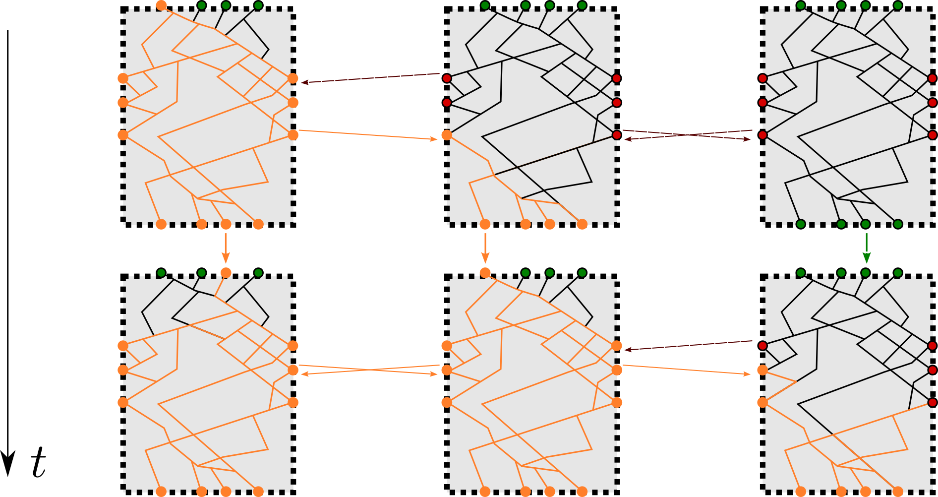
Figure 2: The environment is divided into boxes at different levels. An orange vertex starts infecting everything on its way down. Boxes are well connected since $p$ is large. The infection uses special vertices (outputs/inputs depicted as circles) to spread to other neighbouring boxes. The environment between boxes is hostile, so usually only few connections are found.

The setup for the proof of Theorem 4 is quite long and it is easy to get lost in details. While – as always – the main difficulty lies in those details, they are not as insightful to the general idea and have already been dealt with in other works. We will not reinvent the wheel, but building a cart from it has merit in itself. The procedure is as follows:

1. We move away from Bernoulli random variables in the LoRaC and use geometric ones instead. Both model formulations are equivalent in terms of percolation, but the latter is much more convenient to use.

2. The next step lies in dividing both the time and space random environments into bands.

3. From there, we will use these bands to define $n$ boxes: rectangular subsets in $\mathbb{Z}\times\mathbb{Z}$. These boxes are roughly exponentially large in $n$ and consist of $n-1$ boxes.

4. Each $n$ box has some special vertices on the boundary which we will call (horizontal/vertical) inputs and outputs. There are exponentially many of those vertices.

5. With high probability, $n$ boxes are “good” which means that the aforementioned inputs and outputs are well connected. Also with high probability, the output of an $n$ box will connect to the input of a neighbouring $n$ box (restricted by directionality). This is graphically represented in Figure 2.

6. As $n\to\infty$, the $n$ boxes will always be good which yields an infinite cluster.

We make this procedure rigorous in the next section.

2 Proof skeleton

In the following, we will give the bare proof skeleton leading up to the main result of phase transition. We try to keep the main ideas while omitting most details and proofs.

2.1 Alternative model construction and coupling

We use an alternative, more convenient description of the model. Instead of considering Bernoulli random variables with parameters $q^{(t)}$ and $q^{(x)}$, we directly condense consecutive Bernoulli failures into geometric random variables. Therefore, we will look at the total duration of consecutive lockdowns instead of their existence at a given time. Similarly, we consider distances between houses. The transition from $\mathbb{X}_{x}$ to $N^{(\mathbb{X})}_{x}$ is sketched in Figure 3. In terms of percolation, both constructions are equivalent. One just loses information at which time step exactly a house recovers.

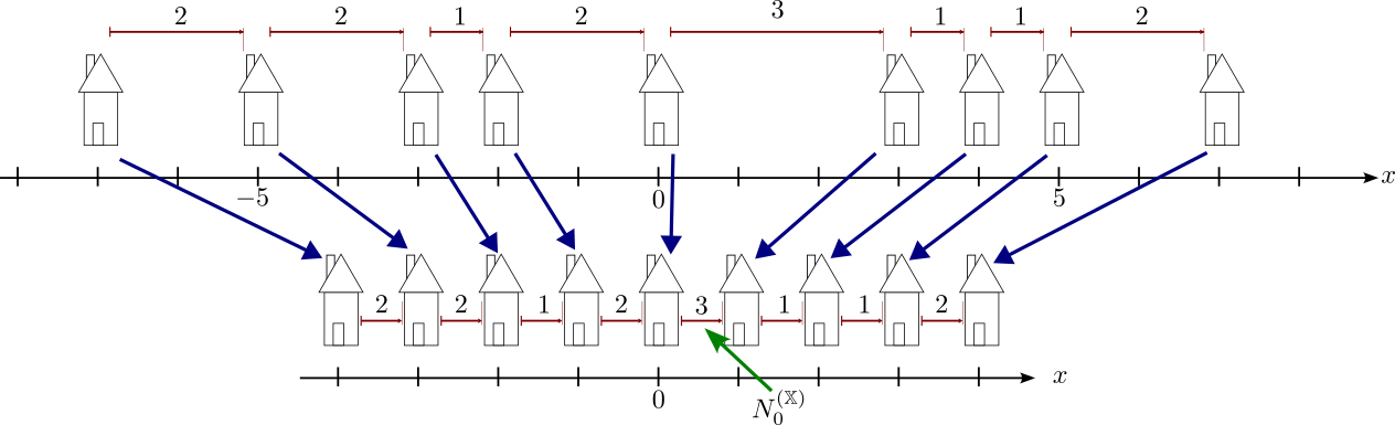
Figure 3: We fix the first existing house starting from $0$ as the new $x=0$ and line up all subsequent houses. Only the distance between houses matters. The same can be analogously done for the lockdowns where we only care about the total duration.

Definition 8 (Alternative construction).

Let $q^{(t)},q^{(x)},p\in(0,1)$ as well as $\alpha>1$ be given. We consider independent sequences of independent geometric random variables $N^{(\mathds{T})}:=(N^{(\mathds{T})}_{t})_{t\in\mathbb{Z}}$ and $N^{(\mathbb{X})}:=(N^{(\mathbb{X})}_{x})_{x\in\mathbb{Z}}$ with parameters $q^{(t)}$ respectively $q^{(x)}$.

Consider the graph $G=(\mathbb{Z}\times\mathbb{Z},E)$ where $E$ consists of directed edges of the form $(t,x)\to(t+1,y)$ with $t,x,y\in\mathbb{Z}$. We consider a mixed bond-site-percolation model on $G$ where – given $N^{(\mathds{T})}$ and $N^{(\mathbb{X})}$ – all vertices and edges are open (respectively closed) independently from each other with probability

$$\mathbb{P}\{(t,x)\text{ is open}\,|\,N^{(\mathds{T})}\}=p^{N^{(\mathds{T})}_{t}}$$ (1)

and

$$\mathbb{P}\{(t,x)\to(t+1,y)\text{ is open}\,|\,N^{(\mathbb{X})}\}=(1+d[x,y,N^{(\mathbb{X})}])^{-\alpha}$$

where $d[x,y,N^{(\mathbb{X})}]$ is the distance between the $x$-th and $y$-th house

$$d[x,y,N^{(\mathbb{X})}]:=\sum_{i=\min(x,y)}^{\max(x,y)-1}N^{(\mathbb{X})}_{i}\,.$$

One realisation of the condensed model is given in Figure 4.

Remark (Beyond geometric random variables).

Note that for the alternative construction to make sense, we do not actually need $N^{(\mathbb{X})},N^{(\mathds{T})}$ to be geometric random variables or even to be $\mathbb{N}-$valued. In fact, it is perfectly reasonable to assume $N^{(\mathbb{X})},N^{(\mathds{T})}\in\mathbb{R}_{>0}^{\mathbb{Z}}$ (which we will actually do in the following rescaling lemmas).

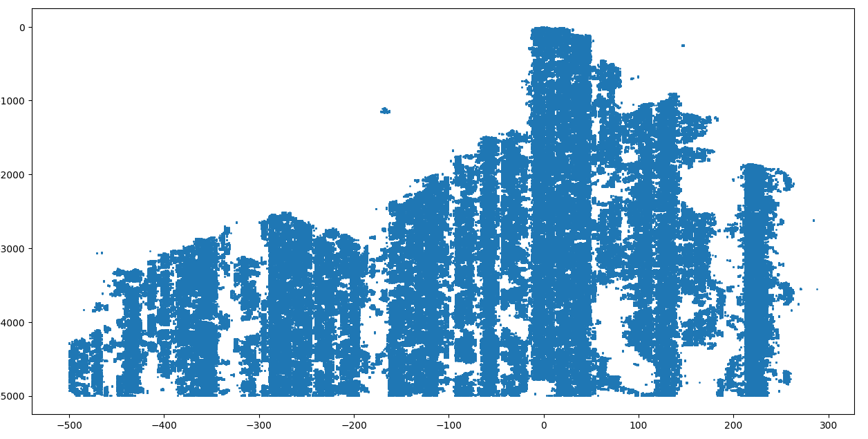
Figure 4: Simulation for $q^{(x)}=q^{(t)}=0.4$, $\alpha=3$ and $p=0.95$ starting with an infected vertex in the origin. One can see distant infections emerging due to long edges. Areas with large $N^{(\mathbb{X})}_{x}$ are easily visible by the vertical gaps, but one can also see thin horizontal gaps where $N^{(\mathds{T})}_{t}$ is large. As the infection spreads in space, it also seems to accelerate albeit often getting stuck at spatial barriers.

The following two coupling lemmas allow us to freely choose the values $q^{(t)}$ and $q^{(x)}$. We will be able to handle arbitrary $\alpha$ by choosing $p$ sufficiently large, so out of the four parameters $q^{(t)},q^{(x)},\alpha,p$, we only need to focus on $p$.

Lemma 9 (Compensate $q^{(t)}$ by $p$).

Let $\gamma>0$. Then, the LoRaC with parameters $\gamma N^{(\mathds{T})}$ and $p^{1/\gamma}$ (with all other values being unchanged) has the same distribution as the one with parameters $N^{(\mathds{T})},p$. In particular, we may assume that $q^{(t)}$ is arbitrarily small by choosing $p$ accordingly close to $1$.

Proof.

This follows immediately from Equation (1). ∎

Lemma 10 (Compensate $q^{(x)}$ via $\alpha$).

Let $\gamma\geq 1$ and consider some finite index set $J\subset\mathbb{Z}$. Then,

$$\Big{(}1+\sum_{i\in J}N^{(\mathbb{X})}_{i}\Big{)}^{-\alpha}\leq\Big{(}1+\sum_{i\in J}\lceil\gamma^{-1}N^{(\mathbb{X})}_{i}\rceil\Big{)}^{-\gamma\alpha}\,.$$

i.e., the LoRaC with parameters $N^{(\mathbb{X})},\alpha$ is stochastically dominated by the process with $\lceil\gamma^{-1}N^{(\mathbb{X})}\rceil,\gamma\alpha$. In particular, we may choose $q^{(t)}$ arbitrarily small by taking $\alpha$ correspondingly large in order to show percolation.

Proof.

For every $a\geq 0$, we prove $(1+a)^{\gamma}\geq 1+\gamma a$. The statement is true for $\gamma=1$. Differentiating in $\gamma$ at $\gamma\geq 1$ yields

$$(1+a)^{\gamma}\cdot\log(1+a)\geq(1+a)\cdot a/(1+a)=a\,,$$

so the statement holds for all $\gamma\geq 1$. Finally,

$$\Big{(}1+\sum_{i\in J}\lceil\gamma^{-1}N^{(\mathbb{X})}_{i}\rceil\Big{)}^{\gamma} \geq 1+\gamma\cdot\sum_{i\in J}\lceil\gamma^{-1}N^{(\mathbb{X})}_{i}\rceil\geq 1+\sum_{i\in J}N^{(\mathbb{X})}_{i}$$

which shows the claim after taking both sides to the power $-\alpha$. ∎

2.2 Environment grouping scheme

Next up is the grouping scheme for the random time and space environments. Due to familiarity, we use the framework of [Hof05] rather than [KSV22]. We extend it for more general values $\mathfrak{s},\mathfrak{d}$ and add extra details to the existing procedure.

We fix two parameters $\displaystyle\mathfrak{s}$ $\displaystyle\geq 32\qquad\text{and}\qquad\mathfrak{d}<1/11\,.$ Consider stretches $N:=(N_{i})_{i\in\mathbb{Z}}$ with $N_{i}\in\mathbb{N}_{\geq 1}\cup\{\infty\}$ where $N_{i}=\infty$ for at most one $i$.

The bottom line is that, if the $N_{i}$ are generated by extremely light-tailed iid geometric random variables, then the grouping scheme terminates almost surely. As a reference, in [Hof05] we have $\mathbb{P}(N_{i}\geq l+1)=(2^{-1000})^{l}$.

Notation.

From now on, $[m,n]$ will be an interval of integers, i.e.,

$$[m,n] :=\{m,\,m+1,\dots,\,n-1,\,n\}\,,$$

$$(m,n) :=[m,n]\backslash\{m,n\}\,.$$

We group indices into bands depending on how “bad” they are. An index $i\in\mathbb{Z}$ is bad if $N_{i}$ is large. These merge into bands which are even “worse”. We do so in a way such that bad bands end up exponentially far apart. Unfortunately, a discount (depending on the distance between far apart bands) has to be introduced for the merging scheme to locally terminate almost surely for geometric $N_{i}$.

We will consecutively define the $k$ bands of $N$, see Figure 5 for a rough illustration.

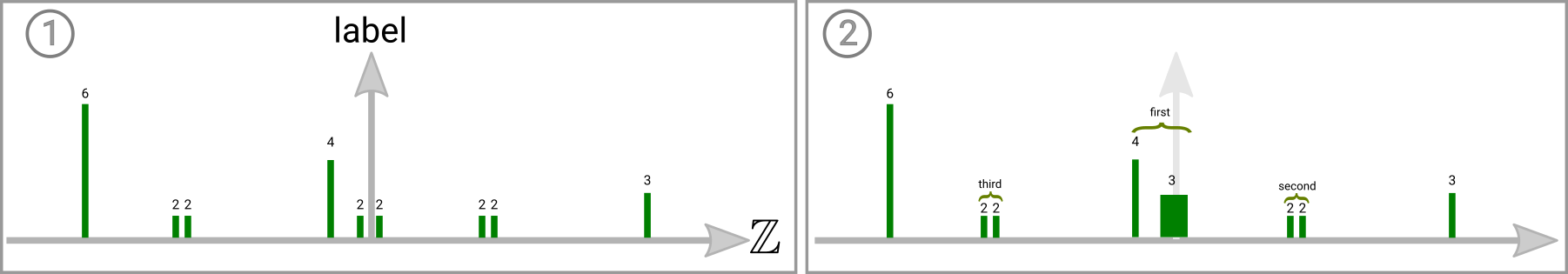
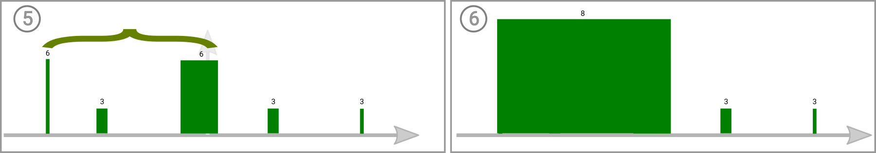
Figure 5: $k$ bands and labels for $k=1,2,5,6$. The base height for labels in the diagrams is $1$. Curly brackets show the merging order of the $k$ bands. After $k=6$, the merging stops locally.

Definition 11 ($k$ bands and $k$ labels).

The $k$ bands and $k$ labels are defined inductively. A $1$ band is $\{i\}$ for $i\in\mathbb{Z}$. The $1$ label of $\{i\}$ is

$$f_{1}(i):=N_{i}\,.$$

For indices $i,j\in\mathbb{Z}$, we set

$$D_{k}(i,j):=\#\{k\text{ bands between }i\text{ and }j\text{ not containing either}\},$$

e.g., at the current step $k=1$, we have $1+D_{1}(i,j)=|i-j|$.

Given a partition of $\mathbb{Z}$ into $k$ bands together with their $k$ labels, the $k+1$ bands and $k+1$ labels are defined in the following way: First, we pick specific merging indices $i,j$ satisfying

$$\min\big{(}f_{k}(i),f_{k}(j)\big{)}-\log_{\mathfrak{s}}\big{(}1+D_{k}(i,j)\big{)}>1\,.$$ (2)

The exact procedure for picking these is given in Algorithm 12. If no such pair exists, we terminate the merging scheme and set all $k+1$ bands and labels to be the same as their $k$ counterpart. Otherwise, using these $i,j$, we update as follows:

1. Let $[m_{i},n_{i}]$ be the $k$ band containing $i$ and $[m_{j},n_{j}]$ the $k$ band containing $j$. Then, $[\tilde{m},\tilde{n}]$ is a $k+1$ band with $\tilde{m}:=\min\{m_{i},m_{j}\}$ and $\tilde{n}:=\max\{n_{i},n_{j}\}$. In this case, all $s\in[\tilde{m},\tilde{n}]$ have the $k+1$ label

   $$f_{k+1}(s):=f_{k}(i)+f_{k}(j)-\left\lfloor\mathfrak{d}\log_{\mathfrak{s}}\big{(}1+D_{k}(i,j)\big{)}\right\rfloor\,.$$ (3)

   Note that $f_{k+1}(s)\geq\max\{f_{k}(i),f_{k}(j)\}+2$.

2. Let $[\tilde{m},\tilde{n}]$ as above. If $[m,n]$ is a $k$ band with $[m,n]\cap[\tilde{m},\tilde{n}]=\emptyset$, then it is also a $k+1$ band. In this case, all $s\in[m,n]$ retain their label $f_{k+1}(s):=f_{k}(s)$.
   Note that this condition is equivalent to $[m,n]\not\subset[\tilde{m},\tilde{n}]$.

Remark (Short summary).

Each $k$ band is an interval of integers. At each step, two $k$ bands and everything inbetween merge into a bigger $k+1$ band of larger label. In Algorithm 12, we see that $k$ bands close to the origin are preferred. For iid geometric $N_{i}$, the merging procedure never terminates globally since there is always something to merge.

Now, let us specify how exactly the merging indices in Definition 11 are chosen.

Algorithm 12 (Finding merging indices).

Consider candidates $i,j\in\mathbb{Z}$ not belonging to the same $k$ band and satisfying Equation 2.

1. First, look for the smallest candidate pair $i,j$, that is, the $i\in\mathbb{Z}$ with the smallest $|i+0.1|$ (i.e., $-|i|$ is preferred over $|i|$) such that $|j|\leq|i|$.

2. If $1+D_{k}(i,j)<(12\mathfrak{s})^{2}$, we choose $i,j$ as our merging indices.

3. If not, we try to look for “better” candidates that are close to $i,j$:

   1. Search for candidates with $i^{\prime},j^{\prime}$ satisfying $1+D_{k}(i^{\prime},j^{\prime})<(12\mathfrak{s})^{2}$ as well as

      $$1+D_{k}(i,j^{\prime})<(12\mathfrak{s})^{2}\qquad\text{or}\qquad 1+D_{k}(j,j^{\prime})<(12\mathfrak{s})^{2}\,,$$

      i.e. $j^{\prime}$ is not too far away from $i$ or $j$, then continue with $i^{\prime},j^{\prime}$ instead of $i,j$. (Note that $j^{\prime}$ may coincide with $i$ or $j$.)

   2. If there are multiple candidates in the previous Step (a), take the $j^{\prime}$ minimizing $|j^{\prime}+0.1|$ and then the $i^{\prime}$ minimizing $D_{k}(i^{\prime},j^{\prime})$. These are our merging indices.

   3. If no such pair $i^{\prime},j^{\prime}\in\mathbb{Z}$ exists, take $i,j$ as the merging indices.

Remark (Better candidates).

The “finding better candidates”-part is new compared to [Hof05] and changes the order of merges. It is relevant for the proof of Theorem 24 Point 3 in the base case of simple bands (Definition 37).

Two things are worth mentioning: First, if two $k$ bands with label $\geq l$ are not at least $\mathfrak{s}^{l-1}$ apart, then they will merge at some point. Second, the size of a $k$ band (in terms of the indices it contains) is limited by its label as seen in the following.

Lemma 13 (Band size limit, [Hof05, Lemma 3.1]).

If $[m,n]$ is a $k$ band with $f_{k}(m)=l$, then $|n-m+1|\leq(\mathfrak{s}/2)^{l-1}$.

An indicated key result is the local termination of the merging scheme for light-tailed $N_{i}$.

Lemma 14 (Exponential decay of band labels, [Hof05, Lemma 3.4]).

Assume that $N=(N_{i})_{i\in\mathbb{Z}}$ is a sequence of iid geometric random variables with $\mathbb{P}(N_{1}\geq l+1)=\mathfrak{q}^{l}$. For any $J\in\mathbb{Z}$, $l\in\mathbb{N}$, and decay $\mathfrak{p}\in(0,1)$, there exists a geometric parameter $\mathfrak{q}:=\mathfrak{q}(\mathfrak{s},\mathfrak{d},\mathfrak{p})\in(0,1)$, such that we have

$$\mathbb{P}\big{(}\exists k\text{ s.t. }J\text{ lies in a }k\text{ band with label }\geq l\big{)}\leq\mathfrak{p}^{l-1}\,.$$

In particular, the following holds almost surely: For each $J\in\mathbb{Z}$, there exists a $K\in\mathbb{N}$ such that for all $k\geq K$, all the $n$ bands containing $J$ are identical.

Since the $k$ bands are static at some point, we may now define the “$k=\infty$” bands.

Definition 15 (Bands and labels).

1. An (integer) interval $[m,n]$ is called a band (without $k$ in front) if there exists some $K\in\mathbb{N}$ such that $[m,n]$ is a $k$ band for all $k\geq K$. For $j\in\mathbb{Z}$, the label of $j$ is $f(j):=\lim_{k}f_{k}(j)$. The label of a band $[m,n]$ is $f(m)$.

2. If $N=(N_{i})_{i\in\mathbb{Z}}$ is such that $\mathbb{Z}$ decomposes into bands that are finite, then we call $N$ good.

Note that bands and their labels are always finite, i.e., $f(m)<\infty$, except for the (potential) band containing $N_{i}=\infty$.

From now on, we only deal with good $N=(N_{i})_{i\in\mathbb{Z}}$.

Corollary 16.

In the setting of Lemma 14, we may with positive probability set $N_{0}=\infty$ without changing the bands of $N$ and only changing the label of the band containing $0$ to $\infty$.

Setting $N^{(\mathds{T})}_{0}=\infty$ means that we consider all vertices of the form $(0,x)$ to be closed. In this way, Corollary 16 allows us to fix $0$ as a “base height” and therefore restrict ourselves to a half space.

Definition 17 (Neighbouring bands and regularity).

We enumerate bands as $B_{m}^{N},m\in\mathbb{Z}$ where $B_{0}^{N}$ is the band containing $0$ and $B_{1}^{N}$ is the band to the right of $B_{0}^{N}$.

• Two bands $B_{m}^{N}$ and $B_{m^{\prime}}^{N}$ are called neighbouring bands with labels $\geq l$ if they both have labels $\geq l$ and there is no band with label $\geq l$ inbetween.

• The good sequence $N=(N_{i})_{i\in\mathbb{Z}}$ is called regular if for all $l$ and all neighbouring bands $B_{m}^{N}$ and $B_{m^{\prime}}^{N}$ with labels $\geq l$, we have $|m-m^{\prime}|\in[\mathfrak{s}^{l-1},\,12\cdot\mathfrak{s}^{l-1})$, i.e., there are at least $\mathfrak{s}^{l-1}-1$ and at most $12\mathfrak{s}^{l-1}-1$ bands between $B_{m}^{N}$ and $B_{m^{\prime}}^{N}$.

A regular sequence is “regular” in the sense that bands with certain labels show up regularly and are not spread too far apart. A good sequence $N=(N_{i})_{i\in\mathbb{Z}}$ can always be made regular by artificially raising individual $N_{i}$ (Lemma 33). We omit further details here since they are not needed to phrase the general proof skeleton. The condition of $|m-m^{\prime}|\geq\mathfrak{s}^{l-1}$ is automatically satisfied:

Lemma 18 ([Hof05, Lemma 3.6]).

If $B_{m}^{N}$ and $B_{m^{\prime}}^{N}$ have label $\geq l$, $m\neq m^{\prime}$, then $|m-m^{\prime}|\geq\mathfrak{s}^{l-1}$.

Proof.

If not, these bands would have merged before. ∎

Our next object of interest is “the space between neighbouring bands” since this is where our model will build up its “bulk” before percolating through bands.

Definition 19 ($l$ segments).

Let $N$ be good and $[i_{1},\,i_{2}],\,[i_{3},\,i_{4}]$ be two neighbouring bands of label $\geq l$ (for $N$). Then we call $(i_{2},i_{3})$ an $l$ segment. We refer to Figure 6 for an illustration of bands and segments for regular $N$.

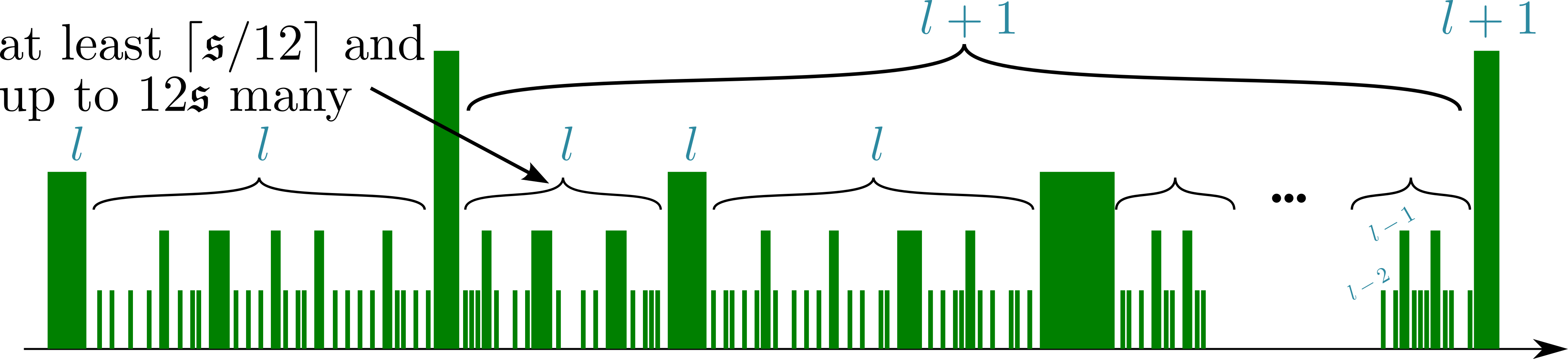
Figure 6: Bands (green bars) and segments (curly brackets) for regular $N$. In this picture, there are always at least four $l$ segments between two neighbouring bands of label $l$.

Lemma 20 (Number of $l$ segments between neighbouring bands).

Let $N$ be regular and $B_{m}^{N},\,B_{m^{\prime}}^{N}$ be neighbouring bands of label $\geq l+1$. Let $\{m_{0},\dots,m_{k}\}=\{\tilde{m}\in[m,m^{\prime}]\,|\,B_{\tilde{m}}^{N}\text{ has label }\geq l\}$. Then, $\lceil\mathfrak{s}/12\rceil\leq k<12\cdot\mathfrak{s}$. In particular, there are between $\lceil\mathfrak{s}/12\rceil$ and $12\cdot\mathfrak{s}$ many $l$ segments separated by bands of label $l$ between two neighbouring bands of label $\geq l+1$.

Proof.

Since $m_{i}-m_{i-1}<12\cdot\mathfrak{s}^{l-1}$ by regularity and $m^{\prime}-m=m_{k}-m_{0}\geq\mathfrak{s}^{l}$, we have $k\cdot 12\cdot\mathfrak{s}^{l-1}\geq\mathfrak{s}^{l}$ which shows the first inequality. The second follows from $m_{i}-m_{i-1}\geq\mathfrak{s}^{l-1}$ and $m^{\prime}-m=m_{k}-m_{0}<12\cdot\mathfrak{s}^{l}$ by the same reasoning. ∎

Apart from the termination of the merging scheme (Lemma 14), the above Lemma 20 is this section’s important take-away. It tells us that we always find a minimal amount of segments between two bands. Regularity gives an upper bound.

2.3 $n$ boxes in $\mathbb{Z}\times\mathbb{Z}$

The framework for the environment grouping has been established. We use it on the temporal environment with parameter $\mathfrak{s}_{t}$ and the spatial one with $\mathfrak{s}_{x}$. Moving along our rough proof outline of Section 1.3, we now use this grouping to build boxes. These boxes will be connected using “inputs” and “outputs” which are just vertices in special locations.

Definition 21 ($n$ boxes, $(m,n)$ strips and $n$ gaps).

• If $[t_{1},t_{2}]$ is a temporal $2$ segment and if $\{x\}$ or $\{x-1\}$ is a spatial band of label $1$, then any rectangle $[t_{1},t_{2}]\times\{x\}$ is a $1$ box. (Equivalently: if for every spatial band $[x_{1},x_{2}]$, we have that $x\notin(x_{1},x_{2}]$.)

• Let $n\in\mathbb{N}_{\geq 2}$. Let $[t_{1},t_{2}]$ be a temporal $n+1$ segment, i.e. the interval between two neighbouring bands with label $n+1$ (see Definition 19), and $(x_{1},x_{2})$ be a spatial $n$ segment. Then, we call

  $$[t_{1},t_{2}]\times(x_{1},x_{2}]$$

  an $n$ box. (Yes, $x_{2}$ included!)

• Let $n\in\mathbb{N}_{\geq 1}$. Let $(t_{2},t^{\prime}_{1})$ be a temporal $n+1$ band and $(x_{1},x_{2})$ be a spatial $m$ segment. Then, we call

  $$(t_{2},t^{\prime}_{1})\times(x_{1},x_{2}]$$

  an $(n+1,m)$ strip. In other words: A $(n+1,n)$ strip is the temporal interruption separating two vertically neighbouring $n$ boxes.

• Let $n\in\mathbb{N}_{\geq 1}$. Let $[t_{1},t_{2}]$ be a temporal $n+1$ segment and $[x_{2},x_{1}^{\prime}]$ be a spatial $n$ band. Then, we call

  $$[t_{1},t_{2}]\times[x_{2},x_{1}^{\prime}]$$

  an $n$ gap. In other words: An $n$ gap is the spatial interruption separating two horizontally neighouring $n$ boxes (starting at the right-most border of the left box).

An illustration of an $n+1$ box is given in Figure 7.

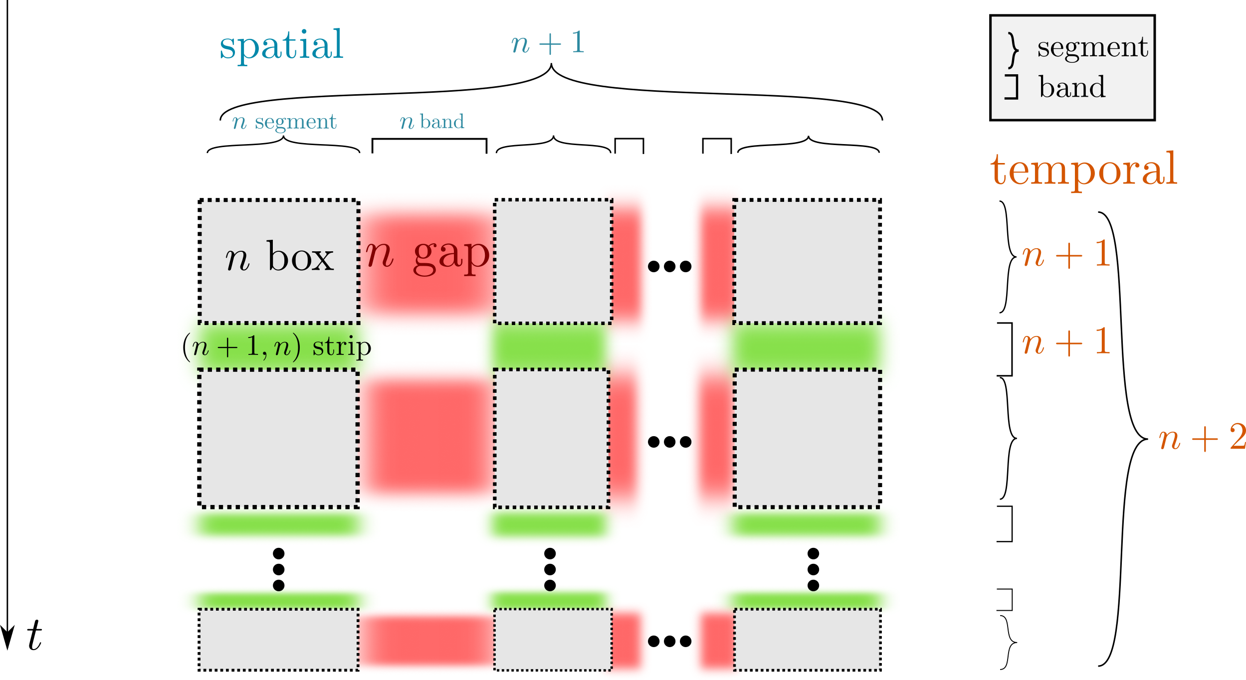
Figure 7: The inner structure of a $n+1$ box. We have grey $n$ boxes with $n$ gaps and $(n+1,n)$ strips between neighbouring boxes. Curly brackets depict segments while square brackets depict bands.

Remark (Renormalisation).

We have to use $n+1$ rather than $n$ bands in the temporal part because we essentially inserted a renormalisation step there. This unfortunately also introduces a lot of bloat in notation. Lemma 20 tells us that an $n+1$ box consists of between $\lceil\mathfrak{s}_{x}/12\rceil+1$ and $12\mathfrak{s}_{x}+1$ many columns as well as between $\lceil\mathfrak{s}_{t}/12\rceil$ and $12\mathfrak{s}_{t}$ many rows of $n$ boxes. These are separated by $n$ gaps respectively $(n,n)$ strips.

Next, we want to formally define good boxes as well as their inputs and outputs now. The directed case makes things a bit more complicated, but the multiscale arguments still work in a nice way. We will often need to connect sets of vertices with each other, so it makes sense to first introduce the following notion (slightly different to [GH02]):

Notation ((Fully) connected sets).

Let $A,B\subset\mathbb{Z}^{2}$ be two sets of vertices. We write

$$A\leadsto B$$

if there are $v\in A,w\in B$ such that $v\leadsto w$, i.e. there exists an open directed path from $v$ to $w$. We write

$$A\leadsto_{\mathrm{ffc}}B$$

if for every $v\in A$ and every $w\in B$, we have $v\leadsto w$. Note that

$$A\leadsto_{\mathrm{ffc}}B\leadsto C\leadsto_{\mathrm{ffc}}D\implies A\leadsto_{\mathrm{ffc}}D\,.$$

Remark.

Before directly moving on to the definition of inputs and outputs, let us recall the basic idea first. Each “good” $n$ box $B_{n}$ will have four sets of vertices $\mathtt{In}^{[\,\shortparallel\,]}(B_{n})$ (on the top), $\mathtt{In}^{[\fallingdotseq]}(B_{n})$ (on the sides), $\mathtt{Out}^{[\fallingdotseq]}(B_{n})$ (also on the sides) and $\mathtt{Out}^{[\,\shortparallel\,]}(B_{n})$ (on the bottom). The $\mathtt{Out}$ stands for outgoing connections to other boxes’ ingoing connections $\mathtt{In}$. For example, $\mathtt{Out}^{[\,\shortparallel\,]}(B_{n})$ stands for vertices which potentially build an open path to $\mathtt{In}^{[\,\shortparallel\,]}(B_{n}^{\prime})$ for another $n$ box $B_{n}^{\prime}$ directly below $B_{n}$. Since the cardinality of these sets grows exponentially in $n$, this means we will have exponentially many trials to bridge an $(n,n)$ strip (and analogously $n$ gaps).

The locations of $\mathtt{In}^{[\fallingdotseq]}(B_{n})$ and $\mathtt{Out}^{[\fallingdotseq]}(B_{n})$ have to be set carefully so that the inputs and outputs are sufficiently well connected inside $B_{n}$. Furthermore, we are only able to make statements on “good” $n$ boxes, so the following definition will appear quite bloated.

Definition 22 (Good $n$ boxes, inputs and outputs).

Let $B_{n}$ be an $n$ box.

• For $n=1$, the $n$ box $B_{n}=[t_{1},t_{2}]\times\{x\}$ is good if all vertices are open (in the sense of Definition 8). In this case, we write $\mathtt{In}^{[\,\shortparallel\,]}(B_{n}):=\{(t_{1},x)\},\mathtt{Out}^{[\,\shortparallel\,]}(B_{n}):=\{(t_{2},x)\}$ as well as

  $$\mathtt{In}^{[\fallingdotseq]}(B_{n}):=(t_{1},t_{2}]\times\{x\}\qquad\text{and}\qquad\mathtt{Out}^{[\fallingdotseq]}(B_{n}):=[t_{1},t_{2})\times\{x\}\,.$$

• An $n$ gap between two horizontally neighbouring boxes $B_{n},B_{n}^{\prime}$ is good if

  $$\mathtt{Out}^{[\fallingdotseq]}(B_{n})\leadsto\mathtt{In}^{[\fallingdotseq]}(B_{n}^{\prime})\qquad\text{and}\qquad\mathtt{Out}^{[\fallingdotseq]}(B_{n}^{\prime})\leadsto\mathtt{In}^{[\fallingdotseq]}(B_{n})\,.$$

• An $(n,n)$ strip between two vertically neighbouring boxes $B_{n},B_{n}^{\prime}$ is good if

  $$\mathtt{Out}^{[\,\shortparallel\,]}(B_{n})\leadsto\mathtt{In}^{[\,\shortparallel\,]}(B_{n}^{\prime})\,.$$

• We call an $n+1$ box $B_{n+1}$ good (and otherwise bad) if the sum of the number of the following bad objects is at most $1$:

  • $n$ boxes inside $B_{n+1}$,

  • $(n+1,n)$ strips between two $n$ boxes inside $B_{n+1}$,

  • $n$ gaps between two $n$ boxes inside $B_{n+1}$.

• In the case of $B_{n+1}$ being good, we first number its $n$ boxes $(B_{i,j})_{1\leq i\leq l_{t},1\leq j\leq l_{x}}$ by their location (with $i=j=1$ being top-left) where $l_{t}\in[\lceil\mathfrak{s}_{t}/12\rceil,\,12\mathfrak{s}_{t}]$ and analogously $l_{x}-1\in[\lceil\mathfrak{s}_{x}/12\rceil,\,12\mathfrak{s}_{x}]$. Next, we set (for some $\kappa[\fallingdotseq]\in\mathbb{N}$ specified in Equation (4))

  $$I:=[0,\kappa[\fallingdotseq]+4)+12\mathfrak{s}_{x}+2\,.$$

  Then, we can finally define the inputs and outputs of the $n+1$ box. The vertical inputs/outputs are as follows: For $j\in\{1,\dots,l_{x}\}$, we set

  $$\mathtt{In}^{[\,\shortparallel\,]}(B_{n+1}) :=\left\{v\in\mathtt{In}^{[\,\shortparallel\,]}(B_{1,j})\,|\,B_{1,j}\text{ is good}\right\}$$

  $$\mathtt{Out}^{[\,\shortparallel\,]}(B_{n+1}) :=\left\{v\in\mathtt{Out}^{[\,\shortparallel\,]}(B_{l_{t},j})\,|\,B_{l_{t},j}\text{ is good }\right\}\,.$$

  Let $\partial B_{n+1}\subset\mathbb{Z}\times\mathbb{Z}$ be the boundary, i.e. the set of all vertices in $B_{n+1}$ having a neighbour outside of it. Then,

  $$\mathtt{In}^{[\fallingdotseq]}(B_{n+1}) :=\big{\{}v\in\mathtt{In}^{[\fallingdotseq]}(B_{i,j})\cap\partial B_{n+1}\,|\,B_{i,j},B_{i+1,j}\text{ are valid, }j\in\{1,l_{x}\},i\in I\big{\}}$$

  $$\mathtt{Out}^{[\fallingdotseq]}(B_{n+1}) :=\big{\{}v\in\mathtt{Out}^{[\fallingdotseq]}(B_{i,j})\cap\partial B_{n+1}\,|\,B_{i-1,j}B_{i,j}\text{ are valid, }j\in\{1,l_{x}\},i\in I\big{\}}$$

  where we say that $n$ boxes $B_{n},B_{n}^{\prime}$ are valid if both are good and $\mathtt{Out}^{[\,\shortparallel\,]}(B_{n})\leadsto\mathtt{In}^{[\,\shortparallel\,]}(B_{n}^{\prime})$.

We refer to Figure 8 for an illustration.

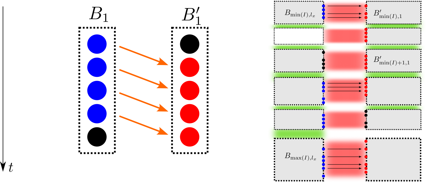
Figure 8: Connecting $\mathtt{Out}^{[\fallingdotseq]}(B_{n+1})$ to $\mathtt{In}^{[\fallingdotseq]}(B_{n+1}^{\prime})$. On the right, we can see that not all $n$ boxes are valid since their respective $\mathtt{In}^{[\fallingdotseq]}/\mathtt{Out}^{[\fallingdotseq]}$ might not be reachable. In that picture, $B_{\min(I)+1,l_{x}}$ is bad (white). Therefore, that sub-box as well as $B_{\min(I)+2,l_{x}}$ do not contribute to $\mathtt{Out}^{[\fallingdotseq]}(B_{n+1})$. For $\mathtt{In}^{[\fallingdotseq]}(B_{n+1}^{\prime})$, it is only $B_{\max(I)-1,1}^{\prime}$ that does not contribute since the gap to $B_{\max(I),1}^{\prime}$ is bad, i.e. $\mathtt{In}^{[\fallingdotseq]}(B_{\max(I)-1,1})$ might not be able to connect to the rest of the $n+1$ box $B_{n+1}^{\prime}$.

The parameters $\mathfrak{s}_{x}$ and $\mathfrak{s}_{t}$ roughly correspond to the width respectively height of the given boxes. Thus, they also influence the number of connectors between boxes: The larger $\mathfrak{s}_{x}$, the larger the number of vertical connectors between vertically neighboured boxes (since the boxes are wider). The same holds for $\mathfrak{s}_{t}$. We will capture the minimal amount of vertical (respectively horizontal) connectors via the parameters $\kappa[\shortparallel]$ and $\kappa[\fallingdotseq]$.

We set the following parameters: $$\kappa[\shortparallel]:=\lceil\mathfrak{s}_{x}/12\rceil-2\qquad\text{and}\qquad\kappa[\fallingdotseq]:=\lceil\mathfrak{s}_{t}/12\rceil-2\cdot(12\mathfrak{s}_{x}+1)-4\,$$ (4) and assume $\kappa[\shortparallel]\geq 64$ (additional conditions on $\kappa[\fallingdotseq]$ are specified later).

Remark.

The spatial parameter $\mathfrak{s}_{x}$ can just be fixed to $12\cdot 66$ to ensure $\kappa[\shortparallel]\geq 64$. The value of $\mathfrak{s}_{t}$ (equivalently $\kappa[\fallingdotseq]$) will however depend $\alpha$ and a small parameter $\mathbbm{p}$ which governs the probability of bad boxes introduced later in Lemma 24. Also, for a rough estimate on the values: We already have

$$\mathfrak{s}_{x} \geq 11\cdot 66+1\geq 700\qquad\text{and}\qquad\mathfrak{s}_{t}\geq 17^{\prime}000\,,$$

so this is quantitively unfeasible.

2.4 Towards proving percolation

The parameters $\kappa[\shortparallel],\kappa[\fallingdotseq]$ had to be set in such a convoluted way to ensure the following connectivity inside good $n$ boxes:

Lemma 23 (Connecting inputs and outputs inside).

Let $n\in\mathbb{N}$. Let $B_{n}$ be a good $n$ box. Then,

$$\mathtt{In}^{[\,\shortparallel\,]}(B_{n}) \leadsto_{\mathrm{ffc}}\mathtt{Out}^{[\fallingdotseq]}(B_{n})$$

$$\mathtt{In}^{[\,\shortparallel\,]}(B_{n}) \leadsto_{\mathrm{ffc}}\mathtt{Out}^{[\,\shortparallel\,]}(B_{n})$$

$$\mathtt{In}^{[\fallingdotseq]}(B_{n}) \leadsto_{\mathrm{ffc}}\mathtt{Out}^{[\,\shortparallel\,]}(B_{n})\,.$$

In particular, if $B_{n}^{\prime}$ is a horizontally neighbouring good $n$ box with the $n$ gap inbetween being good as well, then

$$\mathtt{In}^{[\,\shortparallel\,]}(B_{n})\leadsto_{\mathrm{ffc}}\mathtt{Out}^{[\,\shortparallel\,]}(B_{n}^{\prime})\,.$$

The application of this lemma can be retrospectively seen in Figure 2.

We may finally state the main auxilliary theorem for the multiscale argument. Using the probability of good $n$ boxes, we are then in the state to prove the main theorem on the survival of the infection (Theorem 4).

Lemma 24 (Main auxilliary lemma, [Hof05, Lemma 4.3]).

Let $\mathbbm{p}\in(0,1)$ and $\kappa[\shortparallel]\geq 64$. For all sufficiently large $\kappa[\fallingdotseq]\in\mathbb{N}$ (depending on $\mathbbm{p},\kappa[\shortparallel]$), there exists $p_{c}\in(0,1)$ such that in the LoRaC model for any $p\geq p_{c}$

1. $\mathbb{P}(B_{n}\text{ is good})\geq 1-\mathbbm{p}^{n+1}$ for any $n$ box $B_{n}$.

2. Let $G_{n}$ be a temporal $n$ gap (between two neighbouring $n$ boxes). Then,

   $$\mathbb{P}(G_{n}\text{ is good})\geq 1-\mathbbm{p}^{n+1}\,.$$

3. For an $(n+1,n)$ strip $\bar{S}$ between two $n$ boxes $B_{n},B_{n}^{\prime}$, we have

   $$\mathbb{P}(\bar{S}\text{ is good})\geq 1-\mathbbm{p}^{n+1}\,.$$

Proof outline.

For the reader’s convenience, we will give a brief overview over the main steps. The complete proof will be given in Section 4.

• Point 1 follows from combinatorial estimates (Lemma 45) and induction after proving Point 2 and 3.

• $n$ gaps are exponentially large in $n$ (Lemma 39). Since we have long-range edges, we can guarantee Point 2 by choosing $\kappa[\fallingdotseq]$ large depending on $\alpha$ (Lemma 47). We do so by crossing the whole $n$ gap in a single jump.

• Point 3 follows from the main difficulty of the whole procedure: the “drilling” (Proposition 48). Luckily, the proof in [Hof05] still works here.

∎

Taking Lemma 24 Point 1, we can finally prove the existence of an infinite directed path and in particular the phase transition of the LoRaC in the parameter $p$.

Proof of Theorem 4.

Puzzling everything together is still something.

1. We first take $\mathfrak{s}_{x}=12\cdot 66,\,\mathbbm{p}=1/4$.

2. Using Lemma 10, we may assume at the cost of $\alpha$ that $q^{(x)}$ is sufficiently small such that Lemma 14 holds for $\mathfrak{d}=1/12$, in particular we may use the whole framework of Section 3.

3. Lemma 24 gives us some $\mathfrak{s}_{t}$ and $p_{c}$ for which it holds.

4. Using Lemma 9, we may assume at the cost of $p$ that $q^{(t)}$ is sufficiently small such that Section 3 can be used for that $\mathfrak{s}_{t}$ and $\mathfrak{d}$.

5. Corollary 16 lets us fix base height $0$ for a positive fraction of temporal environments, i.e. $N^{(\mathds{T})}_{0}=\infty$.

6. Next, choose $u=(1,42)\in\mathbb{Z}_{>0}\times\mathbb{Z}$. This lies in some $n$ box for $n$ large enough. By Lemma 24 Point 1 and Borel–Cantelli, there exists some $N_{0}$ such that all the $n$ boxes $B_{n}$ with $n\geq N_{0}$ containing $u$ are good.

7. Now, take any $v\in\mathtt{In}^{[\,\shortparallel\,]}(B_{N_{0}})$. Since $N^{(\mathds{T})}_{0}=\infty$, we have $v\in\mathtt{In}^{[\,\shortparallel\,]}(B_{n})$ for every $n\geq N_{0}$, in particular $v\leadsto_{\mathrm{ffc}}\mathtt{Out}(B_{n})$. Therefore, $v\leadsto w$ for infinitely many $w$. This already yields us an infinite directed path: Set $v_{0}:=v$. Since $v_{0}$ only has finitely many direct successors, we may choose any of these successors $v_{1}$ that has infinitely many $w$ with $v_{0}\to v_{1}\leadsto w$. Inductively continuing this scheme, we obtain an infinite path $v_{0}\to v_{1}\to v_{2}\to\dots$.

8. $N^{(\mathds{T})}=(N^{(\mathds{T})}_{i})_{i\in\mathbb{Z}}$ is an iid sequence, in particular ergodic. So

   $$\mathbb{P}\{N^{(\mathds{T})}\,\text{s.t.}\,\mathbb{P}(\exists v\in\mathbb{Z}^{2},\,v\leadsto\infty\,|N^{(\mathds{T})})=1\}\in\{0,1\}\,.$$

   Since we have proven percolation on a positive fraction of environments, it has to hold for almost all of them.

∎

3 Details: environment grouping

Now, that the rigorous roadmap has been laid out in Section 2, it is time to flesh it out. The main goals in the current sections are:

• Showing Lemma 14, i.e., local termination of the merging scheme.

• Showing how good sequences can always be made regular and even “very regular” (Lemmas 33, 36).

• Introducing the notion of simple bands (Definition 37) and how they are well-behaved (Lemma 39).

• Splitting up very regular bands (Lemma 40).

3.1 Local termination of merging scheme

We start by quantifying the maximal “size” of bands, i.e., giving the proof for Lemma 13.

Proof of Lemma 13.

The statement is true for $l\leq 3$ since it implies $m=n$. Now suppose $[m,n]$ is a $k$ band with $m\neq n$ and $f_{k}(j)=l>3$. Then, there must be some $k^{\prime}<k$ and $m^{\prime},n^{\prime}$ such that the $k^{\prime}$ bands $[m,m^{\prime}]$ and $[n^{\prime},n]$ merge into $[m,n]$. We denote $\underline{l}:=f_{k^{\prime}-1}(m),\,\bar{l}=f_{k^{\prime}-1}(n)$ and $\mathbf{N}:=D_{k^{\prime}}(m^{\prime},n^{\prime})$. Then, there are at most $\mathbf{N}/\mathfrak{s}^{L-1}$ many $k^{\prime}$ bands with labels $L$ between $[m,m^{\prime}]$ and $[n^{\prime},n]$ (otherwise some would have merged). Using the induction hypothesis on the $k^{\prime}$ bands of labels $L$

$$|n- m+1|\leq|m^{\prime}-m+1|+|n^{\prime}-m^{\prime}-1|+|n-n^{\prime}+1|$$

$$\leq (\tfrac{\mathfrak{s}}{2})^{\underline{l}-1}+(\tfrac{\mathfrak{s}}{2})^{\bar{l}-1}+\sum_{L=1}\sum\big{\{}|b^{\prime}-b+1|\,\Big{|}\,[b^{\prime},b]\subset(m^{\prime},n^{\prime})\text{ is }k^{\prime}-1\text{ band with label }L\big{\}}$$

$$\leq (\tfrac{\mathfrak{s}}{2})^{\underline{l}-1}+(\tfrac{\mathfrak{s}}{2})^{\bar{l}-1}+\sum_{L}(\mathbf{N}/\mathfrak{s}^{L-1})\cdot(\tfrac{\mathfrak{s}}{2})^{L-1}\leq(\tfrac{\mathfrak{s}}{2})^{\underline{l}-1}+(\tfrac{\mathfrak{s}}{2})^{\bar{l}-1}+2\mathbf{N}$$

$${}^{(*)}\leq (\tfrac{\mathfrak{s}}{2})^{\max\{\underline{l},\bar{l}\}-1}+(\tfrac{\mathfrak{s}}{2})^{\min\{\underline{l},\bar{l}\}-1}+2\cdot\mathfrak{s}^{\min\{\underline{l},\bar{l}\}-1}\leq\tfrac{4}{\mathfrak{s}}\cdot(\tfrac{\mathfrak{s}}{2})^{\max\{\underline{l},\bar{l}\}}+\tfrac{2}{\mathfrak{s}}\cdot\mathfrak{s}^{\min\{\underline{l},\bar{l}\}}$$

$${}^{(**)}\leq \tfrac{4}{\mathfrak{s}}(\tfrac{\mathfrak{s}}{2})^{l-1}+\tfrac{2}{\mathfrak{s}}\cdot\mathfrak{s}^{\min\{\underline{l},\bar{l}\}}\leq\tfrac{4}{\mathfrak{s}}(\tfrac{\mathfrak{s}}{2})^{l-1}+\tfrac{2}{\mathfrak{s}}\cdot\mathfrak{s}^{l/(2-\mathfrak{d})}$$

$${}^{(***)}\leq \tfrac{4}{\mathfrak{s}}(\tfrac{\mathfrak{s}}{2})^{l-1}+\tfrac{1}{2}\cdot(\tfrac{\mathfrak{s}}{2})^{l-1}\leq(\tfrac{\mathfrak{s}}{2})^{l-1}\,,$$

where $(*)$ follows from Equation 2 being equivalent to $N<\mathfrak{s}^{\min\{\underline{l},\bar{l}\}-1}-1$, $(**)$ uses $l\geq\max\{\underline{l},\bar{l}\}+1$ and $(***)$ uses Equation 3 for

$$l =\max\{\underline{l},\bar{l}\}+\min\{\underline{l},\bar{l}\}-\mathfrak{d}\log_{\mathfrak{s}}(1+\mathbf{N})$$

$$\geq 2\min\{\underline{l},\bar{l}\}-\mathfrak{d}(\min\{\underline{l},\bar{l}\}-1)\geq(2-\mathfrak{d})\min\{\underline{l},\bar{l}\},$$

which yields

$$4\cdot\mathfrak{s}^{l/(2-\mathfrak{d})}\leq(\tfrac{\mathfrak{s}}{2})^{l}\,,$$

(together with $\mathfrak{d}<1/11\leq 2-(1-\log_{32}4)^{-1}\leq 2-(1-\log_{\mathfrak{s}}4)^{-1}$). ∎

Corollary 25 (Combining distant bands, [Hof05, Lemma 3.2]).

If $[m,m^{\prime}]$ and $[n^{\prime},n]$ merge at step $k+1$, then

$$\mathbf{N}:=\#\big{\{}k\text{ bands lying in }(m^{\prime},n^{\prime})\big{\}}\geq\tfrac{2}{3}(n^{\prime}-m^{\prime}-1)\,.$$

Proof.

Let $\mathbf{N}_{l}$ be the number of $k$ bands in $(m^{\prime},n^{\prime})$ with label $l$. Then $\mathbf{N}_{l}\leq\mathbf{N}/(\mathfrak{s}^{l-1})$ since otherwise some would have merged first. Furthermore $\mathbf{N}=\sum_{l}\mathbf{N}_{l}$, so

$$n^{\prime}-m^{\prime}-1 =\sum\big{\{}b^{\prime}-b+1\,|\,[b,b^{\prime}]\text{ is a }k\text{ band in }(m^{\prime},n^{\prime})\big{\}}$$

$$\leq\mathbf{N}_{1}+ \mathbf{N}_{2}+\sum_{l\geq 3}\mathbf{N}/(\mathfrak{s}^{l-1})(\mathfrak{s}/2)^{l-1}\leq\mathbf{N}_{1}+\mathbf{N}_{2}+\mathbf{N}/2\leq\tfrac{3}{2}\mathbf{N,}$$

which shows the claim. ∎

Next we consider generators. They are relevant in this subsection as well as in Section 3.2. Generators of a $k$ band are, loosely speaking, the boundary points of $<k$ bands that are merged to form the final $k$ band.

Definition 26 (Generators of a $k$ band).

Let $[m,n]$ be a $k$ band.

• The $k$ generators of $[m,n]$ are $m$ and $n$.

• For $k^{\prime}<k$, the $k^{\prime}$ generators of $[m,n]$ are the $k^{\prime}$ generators of the $k^{\prime}$ bands containing a $k^{\prime}+1$ generator of $[m,n]$.

• For $1$ generators, we will omit the $1$ and just call them generators.

• We call a generator $g$ a maximal generator if it satisfies the following:

  • If the $k^{\prime}<k$ bands $[m_{1},n_{1}]$, $[m_{2},n_{2}]$ with $g\in[m_{1},n_{1}]$ combine, then $f_{k^{\prime}}(m_{1})\geq f_{k^{\prime}}(m_{2})$.

• One verifies that $k$ bands $B$ always have a maximal generator. Pick the smallest one $\mathfrak{g}_{k}(B)$.

The next lemma limits the possibilities of generators to be spread apart.

Lemma 27 ([Hof05, Lemma 3.3]).

Let $i_{1}<i_{2}<\dots<i_{n}$ be the generators of an $k$ band with

$$\sum_{j=1}^{n}f_{1}(i_{j})=m\,.$$

Then, there exists $C(\mathfrak{s},\mathfrak{d})>0$ such that

$$\sum_{j=2}^{n}\lfloor\log_{2}(i_{j}-i_{j-1}+1)\rfloor\leq C(\mathfrak{s},\mathfrak{d})m\,.$$

Proof.

If $n=1$, we are done. For each $j\in[2,n]$, let $k_{j}$ be the value such that there exists $a$ and $b$ such that the $k_{j}$ bands $[i_{a},i_{j-1}]$ and $[i_{j},i_{b}]$ merge into $[i_{a},i_{b}]$. Let $\mathbf{N}_{j}$ be number of $k_{j}$ bands between $[i_{a},i_{j-1}]$ and $[i_{j},i_{b}]$. By the previous Corollary 25

$$\tfrac{2}{3}(i_{j}-i_{j-1}+1)\leq 1+\mathbf{N}_{j}.$$

We have that $n\leq m/2$ as well as

$$\sum_{j=2}^{n}\lfloor\mathfrak{d}\log_{\mathfrak{s}}(1+\mathbf{N}_{j})\rfloor\leq m\,,$$ (5)

whose proof will be given right after. $\lfloor xy\rfloor\geq x\lfloor y\rfloor-1$ yields the following chain of implication

$$m\geq\sum_{j=2}^{n}\lfloor\mathfrak{d}\log_{\mathfrak{s}}(\tfrac{2}{3}(i_{j}-i_{j-1}+1))\rfloor\geq\sum_{j=2}^{n}\mathfrak{d}\log_{\mathfrak{s}}2\cdot\lfloor\log_{2}(\tfrac{2}{3}(i_{j}-i_{j-1}+1))\rfloor-n$$

$$m\frac{3\log_{2}\mathfrak{s}}{2\mathfrak{d}}\geq\sum_{j=2}^{n}\lfloor\log_{2}(\tfrac{2}{3}(i_{j}-i_{j-1}+1))\rfloor\geq\sum_{j=2}^{n}\lfloor\log_{2}(i_{j}-i_{j-1}+1)\rfloor-n$$

$$m\big{(}\frac{3\log_{2}\mathfrak{s}}{2\mathfrak{d}}+\frac{1}{2}\big{)}\geq\sum_{j=2}^{n}\lfloor\log_{2}(i_{j}-i_{j-1}+1)\rfloor\,.$$

The claim follows from choosing $C(\mathfrak{s},\mathfrak{d}):=\big{(}\frac{3\log_{2}\mathfrak{s}}{2\mathfrak{d}}+\frac{1}{2}\big{)}$. ∎

Proof of Inequality (5).

By the assumption $\sum_{j=1}^{n}f_{1}(i_{j})=m$, we first see that $n\leq m/2$ since $f_{1}(i_{j^{\prime}})\geq 2$ for generators. Equation (3) gives

$$f_{k_{j}+1}(i_{j})=f_{k_{j}}(i_{j-1})+f_{k_{j}}(i_{j})-\lfloor\mathfrak{d}\log_{\mathfrak{s}}(1+\mathbf{N}_{j})\rfloor\,.$$

If for example $\min_{j}k_{j}=k_{j^{\prime}}$ is the smallest, i.e., we first combine $[i_{j^{\prime}-1}]$ and $[i_{j^{\prime}}]$, this would yield

$$m =\sum_{j=1}^{n}f_{1}(i_{j})=\sum_{j=1}^{n}f_{k_{j^{\prime}}}(i_{j})=\sum_{j=2}^{n}f_{k_{j^{\prime}}+1}(i_{j^{\prime}})+\lfloor\mathfrak{d}\log_{\mathfrak{s}}(1+\mathbf{N}_{j^{\prime}})\rfloor\,.$$

Continuing iteratively with $f_{k_{j^{\prime}}+1}$ now instead of $f_{1}$ yields

$$m =f_{k^{\prime}}(i_{j^{\prime}})+\sum_{j=2}^{n}\lfloor\mathfrak{d}\log_{\mathfrak{s}}(1+\mathbf{N}_{j})\rfloor\geq\sum_{j=2}^{n}\lfloor\mathfrak{d}\log_{\mathfrak{s}}(1+\mathbf{N}_{j})\rfloor\,,$$

which finishes the calculation. (Even $f_{k^{\prime}}(i_{j^{\prime}})\geq 2n$ since merges raise labels by at least $2$.) ∎

We are finally in the spot to prove the first milestone: local termination of the merging scheme.

Proof of Lemma 14.

Let $\mathfrak{q}^{1/2}\leq\mathfrak{p}\cdot\mathfrak{s}^{-3C(\mathfrak{s},\mathfrak{d})}/2$ and $l>1$. Assume that $J$ actually lies in a $k$ band with label $\geq$l and generators $i_{1}<\dots<i_{n}$. In the case that $i_{1}=i_{n}=J$, the claim follows

$$\mathbb{P}(f_{1}(J)\geq l)=\mathbb{P}(N_{J}\geq l)=\mathfrak{q}^{l-1}\leq\mathfrak{p}^{l-1}\,.$$

Otherwise, we continue. The $i_{j}$ satisfy by the label updating procedure in Definition 11

$$m:=\sum_{j}^{n}f_{1}(i_{j})\geq l\,.$$

By Lemma 27 above and Lemma 28 below, we have at most $2^{C(\mathfrak{s},\mathfrak{d})m}$ choices for $\lfloor\log_{2}(i_{2}-i_{1}+1)\rfloor,\dots,\lfloor\log_{2}(i_{n}-i_{n-1}+1)\rfloor$.

Given one such choice, we yet again have $2^{(C(\mathfrak{s},\mathfrak{d})+\tfrac{1}{2})m}$ choices for $(i_{2}-i_{1}),\dots(i_{n}-i_{n-1})$:

Set $a_{j}:=\lfloor\log_{2}(i_{j}-i_{j-1}+1)\rfloor$, in particular $i_{j}-i_{j-1}\leq 2^{a_{j}+1}$. There are $2^{a_{j}+1}$ possibilities for each individual $j$, so in total for the whole ensemble $$\prod_{j=2}^{n}2^{a_{j}+1}\leq 2^{C(\mathfrak{s},\mathfrak{d})m+n}\leq 2^{\{C(\mathfrak{s},\mathfrak{d})+1/2\}m}\,.$$

Furthermore, there are at most $(\mathfrak{s}/2)^{l-1}$ possible starting locations for $i_{1}$ since by Lemma 13

$$i_{1}\leq J\leq i_{1}+(\mathfrak{s}/2)^{l-1}-1\,.$$

So in total, we have at most $(\mathfrak{s}/2)^{l-1}\cdot 2^{(2C(\mathfrak{s},\mathfrak{d})+1)m}$ choices for $i_{1},\dots i_{n}$. For each choice of $i_{1},\dots,i_{n}$, there are at most $2^{m}$ choices for $f_{1}(i_{1}),\dots f_{1}(i_{n})$ (by Lemma 28 below), so we have at most

$$(\mathfrak{s}/2)^{l-1}\cdot 2^{(2C(\mathfrak{s},\mathfrak{d})+1)m}\cdot 2^{m}\leq\mathfrak{s}^{3C(\mathfrak{s},\mathfrak{d})m}$$

choices for the combined $i_{j}$ and $f_{1}(i_{j})$. Each such choice has probability $\mathfrak{q}^{m-n}\leq\mathfrak{q}^{m/2}$ since $\mathbb{P}\{f_{1}(i_{j})=s\}\leq\mathfrak{q}^{s-1}$. Therefore, for $\mathfrak{q}^{1/2}\leq\mathfrak{p}\cdot\mathfrak{s}^{-3C(\mathfrak{s},\mathfrak{d})}/2$ (in particular $\mathfrak{q}\leq\mathfrak{p}/2$)

$$\mathbb{P}\big{(} \exists k\text{ s.t. }j\text{ lies in an }k\text{ band with label }\geq l\big{)}\leq\sum_{m\geq l}\big{[}\mathfrak{s}^{3C(\mathfrak{s},\mathfrak{d})}\mathfrak{q}^{1/2}\big{]}^{m}+\mathfrak{q}^{l-1}$$

$$\leq\sum_{m\geq l}(\mathfrak{p}/2)^{m}+(\mathfrak{p}/2)^{l-1}=\mathfrak{p}^{l}\frac{1}{2^{l}(1-\mathfrak{p}/2)}+(\mathfrak{p}/2)^{l-1}\leq 2^{-(l-1)}\cdot\big{[}\mathfrak{p}^{l}+\mathfrak{p}^{l-1}\big{]}\leq\mathfrak{p}^{l-1},$$

as desired. ∎

Here is the auxiliary lemma we previously used.

Lemma 28 (Combinations of sums).

Let $S\in\mathbb{N}$. Then

$$N(S) :=\#\big{\{}(a_{1},\dots,a_{k})\,|\,a_{j}\geq 1,\sum a_{j}=S\big{\}}=2^{S-1}\,,$$

$$\tilde{N}(S) :=\#\big{\{}(a_{1},\dots,a_{k})\,|\,a_{j}\geq 1,\sum a_{j}\leq S\big{\}}\leq 2^{S}-1\,.$$

Proof.

For $S=1$, we have $N(S)=1$. Assume the claim is true for $S$. Then for $S+1$:

$$\tilde{N}(S+1) =\#\big{\{}(a_{1},\dots,a_{k})\,|\,a_{j}\geq 1,\sum a_{j}\leq S+1\big{\}}$$

$$=\#\bigcup_{R\leq S}\big{\{}(a_{1},\dots,a_{k},S+1-R)\,|\,a_{j}\geq 1,\sum a_{j}=R\big{\}}\cup\{(S+1)\}$$

(induction) $$=1+\sum_{R\leq S}2^{R-1}=2^{S}-1$$

On the other hand

$$N(S+1)=\tilde{N}(S+1)-\tilde{N}(S)=2^{S+1}-2^{S}=2^{S}$$

proves the claim. ∎

We have seen in Lemma 13 that the “size” of a band is limited by its label $l$. To cross $n$ gaps in our percolation model, we are more interested in the actual consecutive stretch. It turns out that this is also just an exponential in $l$.

Lemma 29 (Total weight of a band).

Let $[a,b]$ be a band of label $l$. Then,

$$\sum_{i=a}^{b}f_{1}(i)\leq\mathfrak{s}^{l-1}\,.$$

Proof.

We have $f_{1}(i)\leq l$ for every $i\in[a,b]$. Using Lemma 13, we have $|b-a|\leq(\tfrac{\mathfrak{s}}{2})^{l-1}$, so

$$\sum_{i=a}^{b}f_{1}(i)\leq l\cdot(\tfrac{\mathfrak{s}}{2})^{l-1}\leq\mathfrak{s}^{l-1}\,$$

since $l\leq 2^{l-1}$. ∎

Recall from Definition 17 that we may always enumerate the ($k$) bands. The exponential decay in Lemma 14 shows that it is quite rare to encounter bands with high labels close to the origin. This is the reason why we may set $N_{0}:=\infty$ for a positive fraction of environments $N=(N_{i})_{i\in\mathbb{Z}}$.

Lemma 30 (High labels near origin).

Consider the parameter regime of Lemma 14 for $\mathfrak{p}$ small enough such that $24\sum_{l\geq 1}(\mathfrak{s}\mathfrak{p})^{l}<1$. Consider the event

$$A_{l}:=\big{\{}\forall\text{bands }B_{m}^{N}\text{ with }1\leq|m|\leq 12\cdot\mathfrak{s}^{l},\text{ their labels are }\leq l\big{\}}\,.$$

Then,

$$\mathbb{P}(A_{l})\geq 1-24\cdot(\mathfrak{s}\mathfrak{p})^{l}\qquad\text{and}\qquad\mathbb{P}(\cap A_{l})>0\,,$$

in particular, almost surely $A_{l}$ happens infinitely often.

Proof.

By Lemma 14, we have

$$\mathbb{P}\big{(}A_{l}\big{)}\geq 1-\sum_{|m|=1}^{12\cdot\mathfrak{s}^{l}}\mathbb{P}(B_{m}^{N}\text{ has label }>l)\geq 1-24\cdot(\mathfrak{s}\mathfrak{p})^{l}\quad\text{and}\quad\mathbb{P}\big{(}\cap A_{l}\big{)}\geq 1-24\sum_{l=1}^{\infty}(\mathfrak{s}\mathfrak{p})^{l}>0\,.$$

The last statement follows from the Borel–Cantelli lemma. ∎

Proof of Corollary 16.

This follows from Lemma 30 and noting that all other bands are sufficiently far away from $0$ so that they do not merge. ∎

3.2 Regular bands

The next point on the bucket list is making $N$ regular. $N$ being unbounded guarantees the existence of bands of labels $\geq l$ for all $l\in\mathbb{N}$ and that each such band has exactly $2$ neighbours. We omit most proofs since they are identical to the ones in [Hof05].

Lemma 31 (Raising labels of maximal generators, [Hof05, Lemma 3.7]).

Let $N=(N_{i})_{i\in\mathbb{Z}}$ be good. Let $B_{m}^{N}$ be a band of label $l$ and $i^{\prime}\in\mathbb{Z}$ be a maximal generator of $B_{m}^{N}$. If for all bands $B_{m^{\prime}}^{N}$ of label $>l$, we have that $|m-m^{\prime}|\geq\mathfrak{s}^{l}$, then the sequence

$$\tilde{N}_{i}=\begin{cases}N_{i}&i\neq i^{\prime}\\ N_{i}+1&i=i^{\prime}\end{cases}$$

satisfies the following properties:

1. $B_{n,k}^{N}=B_{n,k}^{\tilde{N}}\,\forall n\in\mathbb{Z},k\in\mathbb{N}$, i.e. all $k$ bands are identical and $\tilde{N}$ is also good.

2. If the $k$ label of $B_{n,k}^{N}$ is $t$, then the $k$ label of $B_{n,k}^{\tilde{N}}$ is $t+\mathds{1}\{i^{\prime}\in B_{n,k}^{N}\}$.

In particular, $i^{\prime}$ is still a maximal generator of $B_{m}^{\tilde{N}}$.

Lemma 32 (Making $N$ more regular, [Hof05, Lemma 3.8]).

Let $N$ be good. For each $L\geq 1$, there exists $N^{L}=(N_{i}^{L})_{i\in\mathbb{Z}}$ such that

1. $N\leq N^{L}\leq N^{L+1}$,

2. $B_{m,k}^{N}=B_{m,k}^{N^{L}}$ for all $m\in\mathbb{Z},k\in\mathbb{N}$, and

3. if $B_{m}^{N^{L}}$ and $B_{m^{\prime}}^{N^{L}}$ are neighbouring bands with label $\geq l$ and if $l\leq L$, then

   $$|m-m^{\prime}|\in[\mathfrak{s}^{l-1},\,3\cdot\mathfrak{s}^{l-1})\,.$$

Furthermore, $N^{L}$ can be chosen such that $(N_{i}^{L})_{L\in\mathbb{N}}$ is unbounded for at most one $i$.

Lemma 33 (Making sequences regular, [Hof05, Lemma 3.9]).

Let $N$ be good.

1. There exists a sequence $\tilde{N}\geq N$ such that all the $k$ bands for $\tilde{N}$ are identical to the $k$ bands for $N$ and such that for neighbouring bands $B_{m},\,B_{m^{\prime}}$ of label $\geq l$, we have

   $$|m-m^{\prime}|\in[\mathfrak{s}^{l-1},\,3\cdot\mathfrak{s}^{l-1})\,,$$

   in particular, $\tilde{N}$ is regular. In this case, we have $\tilde{N}=(N_{i})_{i\in\mathbb{Z}}$ with $\tilde{N}_{i}\in\mathbb{N}\cup\{\infty\}$ with at most one $\tilde{N}_{i}=\infty$. (The labels may differ between $N$ and $\tilde{N}$.)

2. There exists a sequence $\tilde{N}\geq N$ such that all the $k$ bands for $\tilde{N}$ are identical to the $k$ bands for $N$ and such that for neighbouring bands $B_{m},\,B_{m^{\prime}}$ of label $\geq l$, we have

   $$|m-m^{\prime}|\in[\mathfrak{s}^{l-1},\,6\cdot\mathfrak{s}^{l-1})\,,$$

   in particular, $\tilde{N}$ is regular. In this case, we have $\tilde{N}=(N_{i})_{i\in\mathbb{Z}}$ with $N_{i}\in\mathbb{N}$. (The labels may differ between $N$ and $\tilde{N}$.)

Proof.

With $N^{L}$ from Lemma 32, we consider

$$N_{i}^{\infty}:=\lim_{L\to\infty}N_{i}^{L}\in\mathbb{N}\cup\{\infty\}\,.$$

We make the following observations:

1. If $N_{i}^{\infty}=\infty$, then $i$ must be the maximal generator of some band $B_{m}^{N}$.

2. $N_{i}^{\infty}=\infty$ for at most one $i$. Otherwise, we would find two separate bands $B_{m}^{N}\ni i$ and $B_{m^{\prime}}^{N}\ni i^{\prime}$. The label of $B_{m}^{N^{L}}$ is bounded from below by $N_{i}^{L}$, respectively $N_{i^{\prime}}^{L}$ for $B_{m^{\prime}}^{N^{L}}$. So for $l>0$ such that $|m-m^{\prime}|<\mathfrak{s}^{l}$ and $L$ such that $\min(N_{i}^{L},\,N_{i^{\prime}}^{L})\geq l$, we would violate Lemma 32 Condition 3, on the minimal distance between bands.

Let $i^{\infty}$ be the value with $N_{i^{\infty}}^{\infty}=\infty$. We set

$$\tilde{N}_{i}=\begin{cases}\lim_{L\to\infty}N_{i}^{L}&i\neq i^{\infty}\\ \infty&i=i^{\infty}\end{cases}\,.$$

By construction, we have that neighbouring bands $B_{m}^{\tilde{N}},\,B_{m^{\prime}}^{\tilde{N}}$ always satisfy

$$|m-m^{\prime}|\in[\mathfrak{s}^{l-1},3\cdot\mathfrak{s}^{l-1})\,,$$

showing the first statement. The second claim follows from choosing $\tilde{N}_{i^{\infty}}:=N_{i}$ instead of $\infty$. ∎

Remark (Manipulations).

The explicit construction to make bands regular as well as Lemma 30 allow us various manipulations on the environment and locations of bands as well as segments.

• In [JJV23], we tweak the construction such that the origin lies not on one of the “border segments”, but rather on the actual inside with at least two $l$ segments distance to the bands of label $\geq l$. Later, this ensures the existence of a circuit around the origin. This is why we always use $12\mathfrak{s}$ for compatibility rather than just $6\mathfrak{s}$.

• In our case here, we will do quite the opposite: On a positive fraction of environments $N^{(\mathds{T})}$, we may set $N^{(\mathds{T})}_{0}:=\infty$ without changing any bands (Corollary 16), effectively considering percolation on the half-plane $\mathbb{Z}_{>0}\times\mathbb{Z}$. Ergodicity then yields the almost-sure existence of an infinite cluster on $\mathbb{Z}\times\mathbb{Z}$.

3.3 Very regular bands and simple bands

Lastly, we need a bit more information about the internal structure of bands. This is needed to obtain crossing probabilities of strips since we will break bands apart again. The short summary for being very regular is: If two $k$ bands combine, then the space between them had to be regular. The $q$ is a parameter of the distance between those bands and will play quite an important role.

Remark ($k$ bands and $n$ segments).

Short reminder that $k$ band refers to the $k$-th merging step while $n$ segment refers to the segment between to neighbouring $(k)$ bands of label $n$.

Definition 34 ($l$ segments (2)).

In addition to Definition 17, we will also call $(i_{2},i_{3})$ an $l$ segment if there is a good sequence $M=(M_{i})_{i\in\mathbb{Z}}$ with

$$M_{i}=N_{i}\quad\forall i\in(i_{2},i_{3})$$

and $(i_{2},i_{3})$ is a $l$ segment for $M$. We call the segment regular if it is generated by a regular sequence $M$.

Remark.

The situation of the following Definition 35 is similar to Figure 6. But since the “neighbouring” $n$ bands combine, they segments and bands inbetween do not have “level” $n-1$ but rather $q$ with $q<n-1$.

Definition 35 (Very regular $k$ bands and $n$ segments).

Let a regular sequence $N$ be given.

1. Any $k$ band that is a singleton $[i,i]$ is very regular.

2. The $1$ segment $\emptyset$ is very regular.

3. Let $[a,d]$ be a $k$ band with label $l$ which was formed by combining the $\tilde{k}$ bands $[a,\,b]$ and $[c,\,d]$ into the $\tilde{k}+1$ band $[a,\,d]$. $[a,\,d]$ is called very regular if there are $b_{1}=b,b_{2},\dots,b_{m}$ as well as $c_{1},c_{2}\dots,c_{m-1},c_{m}=c$ with $m\leq 12\mathfrak{s}$ as well as a $q\geq 1$ such that

   1. All $\tilde{k}$ bands inside the interval $[a,\,d]$ are very regular $\tilde{k}$ bands.

   2. For all $s$, we have that $[b_{s},\,c_{s}]$ is a very regular $q$ segment.

   3. For all $s<m$, we have that $[c_{s},\,b_{s+1}-1]$ is a very regular $\tilde{k}$ band with label $q$.

4. An $n$ segment $\mathcal{S}$ is called very regular if

   1. $\mathcal{S}$ is a regular $n$ segment. (For $n=2$ and $\mathcal{S}=[a,\,b]$, this implies $\mathfrak{s}\leq(b-a)+2<12\mathfrak{s}$.)

   2. All $k$ bands with labels $n-1$ inside $\mathcal{S}$ are very regular.

   3. All $n-1$ segments inside $\mathcal{S}$ are very regular.

5. A band is called very regular if it is a very regular $k$ band for some $k$.

6. A regular sequence $N$ is called very regular if all the bands generated by $N$ are very regular.

The notion of “very regular” allows us to split bands into smaller parts – enabling the induction step in Proposition 48. As in Lemma 33, we make sequences very regular without changing the final band structure.

Lemma 36 (Very regular sequences, [Hof05, Lemma 3.12]).

Let $N$ be good and regular. Then, there exists $\overline{N}\geq N$ such that $\overline{N}$ is very regular and all bands and labels are identical under both $\overline{N}$ and $N$. In particular, we may always replace a regular sequence with a very regular sequence without changing its band structure nor labels.

Proof.

This is an analogon to Lemma 32 and is proven similarly (by establishing a variant of Lemma 31). The labels of the final bands being unchanged follows from the construction: To make bands very regular, one only needs to change the labels of the $k$ bands on the “inside”. But these labels do not contribute to the label of the final combined band. ∎

There is one edge case that we have to worry about due to technical issues: We want to combine bands that are close to each other first. This led to the quite cumbersome merging scheme in Definition 11/Algorithm 12 as well as the following:

Definition 37 (Simple $k$ bands).

1. Any $k$ band that is a singleton $[i,i]$ is simple.

2. Let $[a,d]$ be a $k$ band with label $l$ which was formed by combining the $\tilde{k}$ bands $[a,\,b]$ and $[c,\,d]$ into the $\tilde{k}+1$ band $[a,\,d]$. $[a,\,d]$ is called simple if both $[a,b]$ and $[c,d]$ are simple $\tilde{k}$ bands as well as

   $$1+D_{\tilde{k}}(b,c)<(12\mathfrak{s})^{2}$$

   (see Definition 11, Algorithm 12).

Remark ($q$ in simple bands).

By Definition 37 and Algorithm 12, we see that simple bands satisfy $q\leq 2$ with $q$ as in Definition 35 above. Furthermore, if

$$\mathfrak{s}\geq 72=(12)^{2}/2\,,$$

then this is even an equivalence since for $q=3$, we would automatically have

$$1+D_{\tilde{k}}(b,c)\geq 2\cdot\mathfrak{s}^{3}>(12\mathfrak{s})^{2}\,.$$

(Using that the minimal size of a $3$ segment is $\mathfrak{s}^{2}$.) This allows for an easy characterisation.

Lemma 38 (Sufficient criterion for simple bands).

Let $[a,d]$ be a $k$ band with label $l$ which was formed by combining the $\tilde{k}$ bands $[a,\,b]$ and $[c,\,d]$ into the $\tilde{k}+1$ band $[a,\,d]$. If

$$1+D_{\tilde{k}}(b,c)<(12\mathfrak{s})^{2}\,,$$

then $[a,b]$ and $[c,d]$ also had to be simple $\tilde{k}$ bands. In particular, if $\mathfrak{s}\geq 72$ and $q\leq 2$, then $[a,d]$ is simple.

Proof.

One checks that if either $[a,b]$ or $[c,d]$ have been non-simple, then it would contradict with Step 2 in the construction of $k$ bands in Definition 11. The last statement follows from the previous remark. ∎

The nice thing about simple bands – and the sole reason we need to look at them – is that their “stretch” grows at most linearly in $l$ (rather than the extremely crude exponential estimate in Lemma 29):

Lemma 39 (Maximal stretch of simple bands).

Let $\mathfrak{s}\geq 72$. Let $[a,d]$ be a simple $k$ band with label $l\geq 2$. Then,

$$\sum_{i\in[a,d]}f_{k}(i)\leq l+(13\mathfrak{s})^{2}\cdot(l-2)/2\,.$$

Proof.

In the case of a singleton $[a,d]=[a,a]$, this is true since $f_{k}(a)=l$. Now, assume that the claim is true for all $k$ bands with labels $<l$. If the $k$ band is not a singleton, we split it up into the simple $\tilde{k}$ bands $[a,\,b]$ and $[c,\,d]$ as before with labels $l_{1}$ respectively $l_{2}$, where $l_{1}+l_{2}=l$. Since $[a,d]$ is simple and $\mathfrak{s}\geq 72$, it is very regular with $q\leq 2$. Therefore, there can at most be $12\mathfrak{s}$ bands of label $2$ between $[a,b]$ and $[c,d]$ with the rest being bands of label $1$. Now by the induction hypothesis

$$\sum_{i\in[a,d]}f_{k}(i) =\sum_{i\in[a,b]}f_{\tilde{k}}(i)+\sum_{i\in[c,d]}f_{\tilde{k}}(i)+\sum_{i\in(b,c)}f_{k}(i)$$

$$\leq\big{\{}l_{1}+(13\mathfrak{s})^{2}\cdot(l_{1}-2)/2\big{\}}+\big{\{}l_{2}+(13\mathfrak{s})^{2}\cdot(l_{2}-2)/2\big{\}}+\big{\{}2\cdot 12\mathfrak{s}+(12\mathfrak{s})^{2}\big{\}}$$

$$\leq l+(13\mathfrak{s})^{2}\cdot(l-4)/2+(13\mathfrak{s})^{2}=l+(13\mathfrak{s})^{2}\cdot(l-2)/2\,,$$

which shows the claim. ∎

We conclude the section with parameter estimates on very regular bands. These turn out to be quite crucial, in particular the upper bound for $q$.

Lemma 40 (Estimates for $m,r,q$ on very regular bands).

Assume that we have split the very regular band into bands with labels $m,r$ and have the space inbetween with parameter $q$. Then,

$$m+r=n\quad\forall q\leq 8$$ (6)

as well as

$$m+r-\lfloor\mathfrak{d}q\rfloor=n+\sigma$$ (7)

with $\sigma\in\{-1,0,1\}.$ Furthermore,

$$q\leq\lfloor(2-\mathfrak{d})^{-1}n\rfloor=:\flat(n)\,.$$ (8)

Note that since $\mathfrak{d}<1/11$, we have $\flat(n)\leq\lfloor\tfrac{11}{21}n\rfloor$.

Proof.

We get to return to the label generation again (Definition 11):

$$n=m+r-\lfloor\mathfrak{d}\log_{\mathfrak{s}}(1+D)\rfloor$$

where $D$ is the number of bands between the bands of label $m,r$ right before combining. Since the bands are very regular, we have at most $12\cdot\mathfrak{s}-1$ many bands of label $q$ between them with corresponding $q$ segments. Each $q$ segment contains at least $\mathfrak{s}^{q-1}$ and at most $12\cdot\mathfrak{s}^{q-1}$ many bands. Therefore

$$\mathfrak{s}^{q-1} \leq D\leq 12\cdot\mathfrak{s}^{q-1}\cdot 12\mathfrak{s}+(12\mathfrak{s}-1)$$

$$\mathfrak{s}^{q-1} \leq 1+D\leq\mathfrak{s}^{q}\cdot 13^{2}$$

$$q-1 \leq\log_{\mathfrak{s}}\big{(}1+D\big{)}\leq q+2\log_{\mathfrak{s}}13$$

$$\mathfrak{d}q-\mathfrak{d} \leq\mathfrak{d}\log_{\mathfrak{s}}\big{(}1+D\big{)}\leq\mathfrak{d}q+\mathfrak{d}2\log_{\mathfrak{s}}13\,.$$

If $q\leq 8$, then $\mathfrak{d}q+\mathfrak{d}2\log_{\mathfrak{s}}13<1$, in particular $\lfloor\mathfrak{d}\log_{\mathfrak{s}}(1+D)\rfloor=0$. This proves Equation (6). Furthermore, since $\mathfrak{d}(2\log_{\mathfrak{s}}13+1)\leq\tfrac{1}{11}(1+1)<1$, we have

$$\big{|}\lfloor\mathfrak{d}q\rfloor-\lfloor\mathfrak{d}\log_{\mathfrak{s}}\big{(}1+D\big{)}\rfloor\big{|}\leq 1$$

which yields Equation (7). Since $m,r>q$, we have

$$n+\text{either }0\text{ or }1\geq 2q-\lfloor\mathfrak{d}q\rfloor+2$$

$$n\geq 2q-\mathfrak{d}q=q(2-\mathfrak{d})$$

$$(2-\mathfrak{d})^{-1}n\geq q\,,$$

i.e., Inequality (8) since $q$ is an integer. ∎

Remark (Final remarks).

As alluded to early on, we will use the whole “segment-band” framework for both the temporal rows as well as spatial columns. In the case of the spatial columns, we will attempt to cross bad bands in a single jump, so not much of the inner structure is needed.

The temporal columns are much harder to handle. We will need to exploit that bands are very regular in order use induction. Lemma 40 will also play a crucial role throughout Section 4.5 as it limits us in how thin we can make strips. The notion of simple bands is needed for the base case of $q\leq 2$.

4 Details: proving percolation

We employ the band/segment grouping scheme for the time/space stretches $(N^{(\mathds{T})}_{t})_{t\in\mathbb{Z}}$, $(N^{(\mathbb{X})}_{x})_{x\in\mathbb{Z}}$ with parameters $\mathfrak{s}_{t},\mathfrak{s}_{x}$ and $\mathfrak{d}=1/12$. We may assume without loss of generality that these stretches are very regular (Lemma 33, 36).

4.1 Connectivity inside/between good boxes

The usual idea with multiscale/block arguments is to connect boxes of different levels with each other. Directionality adds bloat to the proofs, but the principle behind is actually simple and graphical:

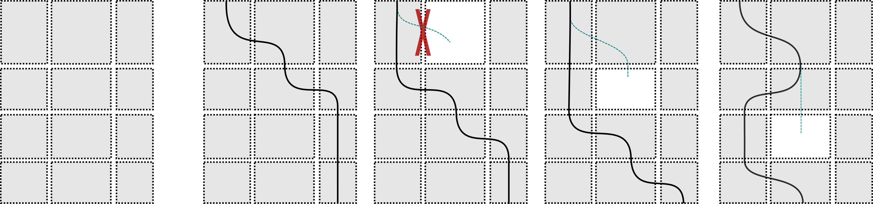
Figure 9: Depicted are the schemes by which we connect boxes. In the best case, we just go to the target column and move straight down. Otherwise, we have to dodge bad boxes/connections.

Lemma 41 (Reachable boxes).

Let a rectangular area of $l_{x}\geq 2$ columns and $l_{t}$ rows of $n$ boxes be given, which are separated by $n$ gaps and $(n+1,n)$ strips. Number them by

$$(B_{i,j})_{1\leq i\leq l_{t},1\leq j\leq l_{x}}\,.$$

Assume that Lemma 23 is true for $n$. If at most one of the $n$ boxes, $n$ gaps or $(n+1,n)$ strips is bad, then for any good $n$ boxes $B_{i,j}$ and $B_{i^{\prime},j^{\prime}}$ with $(i^{\prime}-i)\geq l_{x}$, we have

$$\mathtt{In}^{[\,\shortparallel\,]}(B_{i,j})\leadsto_{\mathrm{ffc}}\mathtt{Out}^{[\,\shortparallel\,]}(B_{i^{\prime},j^{\prime}})\,.$$

Proof.

Without loss of generality, we assume that $j\leq j^{\prime}$, otherwise we mirror the whole procedure. We sketch the connecting procedure in Figure 9 where horizontal connections are made via

$$\mathtt{In}^{[\,\shortparallel\,]}(B_{k,l})\leadsto_{\mathrm{ffc}}\mathtt{Out}^{[\fallingdotseq]}(B_{k,l})\leadsto\mathtt{In}^{[\fallingdotseq]}(B_{k,l+1})\leadsto_{\mathrm{ffc}}\mathtt{Out}^{[\,\shortparallel\,]}(B_{k,l+1})$$

and vertical ones via $\mathtt{Out}(B_{k,l})\leadsto\mathtt{In}(B_{k+1,l})$. First of all, it suffices to only look at the case with at most one bad box: If the gap between $B_{k,l}$ and $B_{k,l+1}$ is bad, we simply declare $B_{k,l}$ to be bad (if it is not the starter box, otherwise take $B_{k,l+1}$). The same works for strips. We distinguish two cases.

1. The procedure is straight-forward. If we are currently in $\mathtt{In}^{[\,\shortparallel\,]}(B_{k,l})$ with $l<j^{\prime}$ and both $B_{k,l+1}$, $B_{k+1,l+1}$ are good, then move towards $\mathtt{Out}^{[\,\shortparallel\,]}(B_{k,l+1})$ (and then $\mathtt{In}^{[\,\shortparallel\,]}(B_{k+1,l+1})$). Otherwise, simply move down $\mathtt{In}^{[\,\shortparallel\,]}(B_{k,l})\leadsto\mathtt{In}^{[\,\shortparallel\,]}(B_{k+1,l})$ and proceed.

2. If $l=j^{\prime}$ – i.e. we have reached the target column $j^{\prime}$ – and $B_{k+1,l}$ is good, then again $\mathtt{In}^{[\,\shortparallel\,]}(B_{k,l})\leadsto\mathtt{In}^{[\,\shortparallel\,]}(B_{k+1,l})$. Otherwise, dodge to side, i.e. $\mathtt{In}^{[\,\shortparallel\,]}(B_{k,l})\leadsto\mathtt{In}^{[\,\shortparallel\,]}(B_{k+1,l+\sigma})$ with $\sigma=1$ if $l=1$ and $-1$ otherwise.

Since at most one box is bad, only one “delaying case” can happen, so we still reach the target output. ∎

Now, we know that rectangular regions of good $n$ boxes are well-connected, given that Lemma 23 holds. Naturally, we have to prove said lemma now for $n=1$ and $n+1$.

Proof of Lemma 23.

This is true for $n=1$. For $n+1$, the claim on $B_{n}$ follows from Lemma 41 and Equation (4) on $\mathfrak{s}_{x},\mathfrak{s}_{t}$: We again number the boxes in $B_{n}$ as $(B_{i,j})_{1\leq i\leq l_{t},1\leq j\leq l_{x}}$ and take some $v\in\mathtt{In}^{[\,\shortparallel\,]}(B_{n})$, in particular $v\in\mathtt{In}^{[\,\shortparallel\,]}(B_{1,j})$. If $w\in\mathtt{Out}^{[\fallingdotseq]}(B_{n})$, then in particular $w\in\mathtt{Out}^{[\fallingdotseq]}(B_{i,j^{\prime}})$ for some $B_{i,j^{\prime}}$. Furthermore, both $B_{i,j^{\prime}}$ and $B_{i-1,j^{\prime}}$ are good (by definition of $\mathtt{Out}^{[\fallingdotseq]}(B_{n})$) with

$$i-1\geq 12\mathfrak{s}_{x}+1\geq l_{x}\,.$$

Using Lemma 41 and the induction hypothesis, we connect $v\leadsto_{\mathrm{ffc}}\mathtt{Out}^{[\,\shortparallel\,]}(B_{i-1,j^{\prime}})\leadsto\mathtt{In}^{[\,\shortparallel\,]}(B_{i,j^{\prime}})\leadsto_{\mathrm{ffc}}\mathtt{Out}^{[\fallingdotseq]}(B_{i,j^{\prime}})$. This proves the first part. The second part follows directly from Lemma 41 and the third part works analogously to the first part. Finally,

$$A\leadsto_{\mathrm{ffc}}B\leadsto C\leadsto_{\mathrm{ffc}}D\implies A\leadsto_{\mathrm{ffc}}D\,,$$

yields the final statement on neighbouring boxes. ∎

4.2 Connecting outputs with inputs and multiscale estimates

Not all outputs of $n$ boxes connect directly to inputs. There is always some loss due to bad $n-1$ boxes in prior steps. In this subsection, we quantify the minimum amount of suitable connectors, which yields the probability of good $(n+1,n)$ strips as well as $n$ gaps.

Definition 42 ($(\kappa[\shortparallel],n)$ trees).

1. A $(\kappa[\shortparallel],1)$ tree is any single vertex.

2. A $(\kappa[\shortparallel],n)$ tree consists of $\kappa[\shortparallel]$ many disjoint $(\kappa[\shortparallel],n-1)$ trees such that they all lie inside $\{t\}\times(x_{1},x_{2}]$ for some some $t\in\mathbb{Z}$ and spatial $n$ segment $(x_{1},x_{2})$.

Remark.

$(\kappa[\shortparallel],n)$ trees capture the basic shape of the sets $\mathtt{In}^{[\,\shortparallel\,]}(B_{n})$ and $\mathtt{Out}^{[\,\shortparallel\,]}(B_{n})$ of an $n$ box $B_{n}$. Each such tree contains (exactly) $\kappa[\shortparallel]^{n-1}$ many vertices. They will play the role of “connectors” between vertically neighbouring boxes as we see in the following:

Lemma 43 ($(\kappa[\shortparallel],n)$ trees between good $n$ boxes).

Let $B_{n}$ and $B_{n}^{\prime}$ be $n$ boxes where $B_{n}$ lies on top of $B_{n}^{\prime}$ (only separated by an $(n+1,n)$ strip). Then, they define at least one $(\kappa[\shortparallel],n)$ tree $T$ such that:

$$T\subset\mathtt{Out}^{[\,\shortparallel\,]}(B_{n})\qquad\text{and}\qquad\pi_{x}(T)\subset\pi_{x}(\mathtt{In}^{[\,\shortparallel\,]}(B_{n}^{\prime}))$$

where $\pi_{x}:\mathbb{Z}^{2}\to\mathbb{Z}$ is the projection onto the $x$-coordinate. In words: They define a $(\kappa[\shortparallel],n)$ tree $T$ such that $T$ lies in the same column as $\mathtt{Out}(B_{n})$ and $\mathtt{In}(B_{n}^{\prime})$.

Proof.

The proof is by induction. In the case a $1$ box $B_{n}=[t_{1},t_{2}]\times\{x\}$ we take $T=\{(t_{2},x)\}$. For general $n$, we know that in each row of these at least $\kappa[\shortparallel]+2$ many $n-1$ boxes, at most one of these boxes is bad. Therefore, there are at least $\kappa[\shortparallel]$ many pairs of good vertically neighboured $n-1$ boxes. By the induction hypothesis, these define $\kappa[\shortparallel]$ many $(\kappa[\shortparallel],m-1)$ trees which satisfy Condition 2 of Definition 42 above since they lie in $B_{n}$. Therefore, we obtain a $(\kappa[\shortparallel],n)$ tree as claimed. ∎

This covers the case of vertical connectors. We set up the same framework analogously for horizontal connectors, but actually keep things straight and explicit here:

Lemma 44 (Number of horizontal connectors between good $n$ boxes).

Let $B_{n},B_{n}^{\prime}$ be neighbouring good $n$ boxes. Then, there are at least $\kappa[\fallingdotseq]^{n}$ many edges from $\mathtt{Out}^{[\fallingdotseq]}(B_{n})$ to $\mathtt{In}^{[\fallingdotseq]}(B_{n}^{\prime})$ crossing exactly over the $n$ gap inbetween..

Proof.

In the case of $1$ boxes $B_{1}=[t_{1},t_{2}]\times\{x\},\,B_{1}^{\prime}=[t_{1},t_{2}]\times\{x^{\prime}\}$, every $(t,x)\in\mathtt{Out}^{[\fallingdotseq]}(B_{1})$ has an outgoing edge to $(t+1,x^{\prime})\in\mathtt{In}^{[\fallingdotseq]}(B_{2})$ for every $t\in[t_{1},t_{2})$. This makes $|t_{2}-t_{1}|\geq\lceil\mathfrak{s}_{t}/12\rceil-1\geq\kappa[\fallingdotseq]$ many different edges.

For the case of the $n+1$ boxes $B_{n+1},B_{n+1}^{\prime}$, we see by the definition of inputs/outputs (in Definition 22) that $\mathtt{Out}^{[\fallingdotseq]}(B_{n+1})$ and $\mathtt{In}^{[\fallingdotseq]}(B_{n+1}^{\prime})$ consist of $\kappa[\fallingdotseq]+4$ many opposing $n$ boxes if they were all valid. Since $B_{n+1},B_{n+1}^{\prime}$ are good, at most $2$ of the the boxes in $\mathtt{Out}^{[\fallingdotseq]}(B_{n+1})$ might not be valid, same for $\mathtt{In}^{[\fallingdotseq]}(B_{n+1}^{\prime})$. Therefore, we have $\kappa[\fallingdotseq]$ many opposing $n$ boxes that may connect with each other. By the induction hypothesis, each of these contribute at least $\kappa[\fallingdotseq]^{n}$ many edges, so we have $\kappa[\fallingdotseq]\cdot\kappa[\fallingdotseq]^{n}=\kappa[\fallingdotseq]^{n+1}$ in total which proves the claim. ∎

With this, we have guaranteed that there are exponentially many potential connectors for both the vertical strips as well as horizontal gaps. This is important since we want to use the following estimate:

Lemma 45 (Combinatorial estimate).

Assume there is a collection of at most $C$ “objects” that are each good with probability at least $P_{n}$ independently from each other. Furthermore, assume that a certain object of level $n+1$ is good if at most one of the $C$ prior objects is bad. Then, for any $\mathbbm{p}\in(0,1)$ with $\mathbbm{p}^{n+1}\leq C^{-6}$, if $n\geq 1$ and

$$1-P_{n}\leq\mathbbm{p}^{n+1}\,,$$

then also

$$1-P_{n+1}\leq\mathbbm{p}^{n+2}\,.$$

Proof.

We first write $1+k_{n}:=(1-P_{n})^{-1}$. The level $n+1$ object is good with probability at least

$$P_{n+1}\geq(P_{n})^{C}+C\cdot(P_{n})^{C-1}\cdot(1-P_{n})\,.$$

Therefore

$$1-P_{n+1}\leq 1-\left[\left(\frac{k_{n}}{1+k_{n}}\right)^{C}+C\cdot\left(\frac{k_{n}}{1+k_{n}}\right)^{C-1}\cdot\frac{1}{1+k_{n}}\right]=\frac{(k_{n}+1)^{C}-(k_{n})^{C}-C\cdot(k_{n})^{C-1}}{(1+k_{n})^{C}}\,.$$

The subtrahends are exactly the first two terms in this binomial expression. Therefore,

$$1-P_{n+1}=(1+ k_{n})^{-C}\cdot\sum_{i=0}^{C-2}{C\choose i}(k_{n})^{i}\leq\frac{C^{3}\cdot(1+k_{n})^{C-2}}{(1+k_{n})^{C}}$$

$$\leq(1+k_{n})^{-1.5}\leq(1-P_{n})^{1.5}\leq\mathbbm{p}^{(n+1)\cdot 1.5}\leq\mathbbm{p}^{n+2}\,,$$

where we also used $1+k_{n}=(1-P_{n})^{-1}\geq\mathbbm{p}^{-(n+1)}\geq C^{6}$. ∎

Remark.

The lemma can be generalised to allow for $C[n]=a_{1}\mathrm{e}^{a_{2}n}$ instead of a constant $C$.

In our case, the “level $n+1$” object will be an $n+1$ box containing up to $C$ many $n$ boxes, $(n+1,n)$ strips as well as $n$ gaps inbetween. By construction, each $n+1$ box will then contain at most $(12\mathfrak{s}_{x}+1)\cdot 12\mathfrak{s}_{t}$ many $n$ boxes, so the total number of level $n$ objects is

$$C\leq(12\mathfrak{s}_{x}+1)\cdot 12\mathfrak{s}_{t}\cdot(1+1+1)\leq 450\cdot\mathfrak{s}_{x}\mathfrak{s}_{t}\,.$$ (9)

There is a small technical issue in using Lemma 45: In order to ensure a high probability for $n$ gap crossings, we need a large amount of connectors, i.e. $\mathfrak{s}_{t}$ to be large. But this also results in a larger constant $C$, so the gap crossing probability has to grow accordingly. The next two lemmas ensure that this circular dependency is not a problem.

Lemma 46 (Horizontal strip crossing).

Let $B_{n}$ and $B_{n}^{{}^{\prime}}$ be neighbouring good $n$ boxes. Then

$$\mathbb{P}\big{\{}\mathtt{Out}^{[\fallingdotseq]}(B_{n})\not\leadsto\mathtt{In}^{[\fallingdotseq]}(B_{n}^{\prime})\big{\}}\leq\exp\big{(}-\{(1+\mathfrak{s}_{x})^{-\alpha}\kappa[\fallingdotseq]\}^{n}\big{)}\,.$$

Proof.

By Lemma 44, there are at least $\kappa[\fallingdotseq]^{n}$ suitable edges that would connect $\mathtt{Out}^{[\fallingdotseq]}(B_{n})$ with $\mathtt{In}^{[\fallingdotseq]}(B_{n}^{\prime})$ if they were open. By Lemma 29, these edges have length at most $\mathfrak{s}_{x}^{n}$. Therefore

$$\mathbb{P}\big{\{}\mathtt{Out}^{[\fallingdotseq]}(B_{n}) \not\leadsto\mathtt{In}^{[\fallingdotseq]}(B_{n}^{\prime})\big{\}}\leq\big{(}1-\{1+\mathfrak{s}_{x}^{n}\}^{-\alpha}\big{)}^{(\kappa[\fallingdotseq]^{n})}\leq\exp\big{(}-\{1+\mathfrak{s}_{x}\}^{-n\alpha}\cdot\kappa[\fallingdotseq]^{n}\big{)}$$

$$\leq \exp\big{(}-\{(1+\mathfrak{s}_{x})^{-\alpha}\kappa[\fallingdotseq]\}^{n}\big{)}\,,$$

which yields the claim. ∎

Lemma 47 (Ensuring high probability of horizontal strip crossings).

Given fixed $\mathbbm{p}$, $\mathfrak{s}_{x}$ and $\alpha$, then we have for $\mathfrak{s}_{t}$ large enough (equivalently $\kappa[\fallingdotseq]$ large enough): For any $n$ gap $G$, we have

$$1-\mathbb{P}(G\text{ is good})\leq\min\left\{\mathbbm{p}^{n+1},\left(450\cdot\mathfrak{s}_{x}\mathfrak{s}_{t}\right)^{-6}\right\}\,.$$

In particular, we may ensure that both Theorem 24 Point 2 as well as the requirements of Lemma 45 hold for horizontal gaps.

Proof.

Using the previous lemma, we see that we only need to show

$$2\exp\big{(}-\{(1+\mathfrak{s}_{x})^{-\alpha}\kappa[\fallingdotseq]\}^{n}\big{)}\leq\min\left\{\mathbbm{p}^{n+1},\left(450\cdot\mathfrak{s}_{x}\mathfrak{s}_{t}\right)^{-6}\right\}\,.$$

First, by Equation (4)

$$\kappa[\fallingdotseq]\geq\mathfrak{s}_{t}/12-25\mathfrak{s}_{x}=\mathfrak{s}_{t}/12-c\,,$$

so the requirements on horizontal crossings are met if both

$$2\exp\big{(}-\big{\{}(1+\mathfrak{s}_{x})^{-\alpha}(\mathfrak{s}_{t}/12-c)\big{\}}^{n}\big{)}\leq\exp\big{(}-\big{\{}(1+\mathfrak{s}_{x})^{-\alpha}\kappa[\fallingdotseq]\big{\}}^{n}\big{)}\leq\left(450\cdot\mathfrak{s}_{x}\mathfrak{s}_{t}\right)^{-6}$$

and

$$\exp\big{(}-\big{\{}(1+\mathfrak{s}_{x})^{-\alpha}\kappa[\fallingdotseq]\big{\}}^{n}\big{)} \leq\mathbbm{p}^{n+1}$$

$$\big{\{}(1+\mathfrak{s}_{x})^{-\alpha}\kappa[\fallingdotseq]\big{\}}^{n} \geq(n+1)\log\tfrac{1}{\mathbbm{p}}$$

are satisfied, which is true for $\mathfrak{s}_{t}$ (equivalently $\kappa[\fallingdotseq])$ large enough. ∎

4.3 Proof of Lemma 24

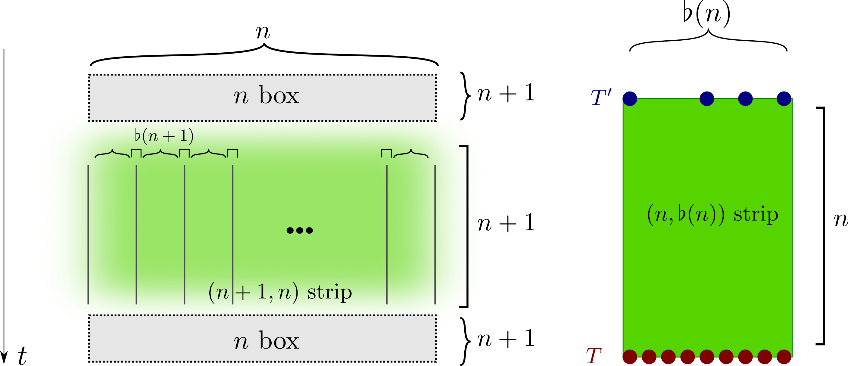
Figure 10: As always, curly brackets indicate bands with the square brackets indicating bands. Whenever we consider a crossing of a $(n+1,n)$ strip, we actually try to do so in disjoint $(n+1,\flat(n+1))$ strips. Since these are “thin” objects, they may be broken down further, so we pay special attention to $(n,\flat(n))$ strips.

We can now prove Lemma 24 provided that Proposition 48 below holds for $n+1$. The setting is depicted in Figure 10.

Proposition 48 (Drilling).

Let $S$ be a $(n,\flat(n))$ strip with $n\geq 1$. Let $T^{\prime}$ be a collection of $(\kappa[\shortparallel],k)$ trees on top of $S$ and $T$ be a $(\kappa[\shortparallel],\flat(n))$ tree on the bottom of $S$ with $\pi_{x}(T^{\prime})\subset\pi_{x}(T)$ where $\pi_{x}$ is the projection onto the $x$-coordinate. Then,

$$\mathbb{P}(\exists\text{ a crossing of }S\text{ intersecting both }T\text{ and }T^{\prime})\geq\kappa[\shortparallel]^{-\flat(n)}\cdot\#T^{\prime}\,.$$

Proof of Theorem 24.

Using Lemma 47, Point $2$ is ensured by fixing some large $\kappa[\fallingdotseq]$ (or equivalently $\mathfrak{s}_{t})$. WLOG, we assume $\mathbbm{p}\leq(450\cdot\mathfrak{s}_{x}\mathfrak{s}_{t})^{-6}$ (for Lemma 45). Then, we choose $p$ large enough such that Lemma 24 holds for every $n\leq\mathcal{N}$, where $\mathcal{N}$ comes from Equation (10) below. We also require $p^{100\mathfrak{s}_{t}{}^{2}}(1-e^{-1})\geq\kappa[\shortparallel]^{-1/2}$ in Equation (11).

1. We show that Point 3 holds for $n$ given that Proposition 48 holds for $n+1$. Let $\mathcal{N}\in\mathbb{N}$ large enough such that

   $$\kappa[\shortparallel]^{n-\flat(n)-2}\geq(n+1)\log\tfrac{1}{\mathbbm{p}}$$ (10)

   for every $n\geq\mathcal{N}$. We use Lemma 43 to first get a $(\kappa[\shortparallel],n)$ tree $\tilde{T}\subset\mathtt{Out}^{[\,\shortparallel\,]}(B_{n})$ with $\pi_{x}(\tilde{T})\subset\pi_{x}(\mathtt{In}^{[\,\shortparallel\,]}(B_{n}^{\prime}))$. Now, the $(n+1,n)$ strip can be divided into $(2+\kappa[\shortparallel])^{n-\flat(n+1)}$ many $(n+1,\flat(n+1))$ strips. We will choose (exactly) $\kappa[\shortparallel]^{n-\{\flat(n)+1\}}$ disjoint $(n+1,\flat(n+1))$ strips $S$ such that they have a $(\kappa[\shortparallel],\flat(n+1))$ tree $T^{\prime}$ on top satisfying $T^{\prime}\subset\tilde{T}$. By Proposition 48, the probability of crossing $S$ is at least $\kappa[\shortparallel]^{-\flat(n+1)}\cdot\#T^{\prime}=1/\kappa[\shortparallel]$. Since all those strips are disjoint, these events are independent. Therefore, we have

   $$\mathbb{P}\big{\{}\nexists\text{ a crossing of } \bar{S}\text{ intersecting }\mathtt{Out}^{[\,\shortparallel\,]}(B_{n}),\mathtt{In}^{[\,\shortparallel\,]}(B_{n}^{\prime})\big{\}}$$

   $$\leq \left(1-1/\kappa[\shortparallel]\right)^{\kappa[\shortparallel]^{n-\flat(n+1)}}\leq\exp\big{(}-\kappa[\shortparallel]^{n-\flat(n)-2}\big{)}\leq\mathbbm{p}{}^{n+1},$$

   which shows Point 3.

2. Showing Point 1 for $n+1$ is a straight-forward application of Lemma 45 after using all the estimates on $n$ boxes, $(n+1,n)$ strips and $n$ gaps.

∎

Judging by the remaining pages, one can guess that Proposition 48, i.e., drilling, is the most difficult part. Also the fact that we have yet to use that $N^{(\mathds{T})}$ is very regular. The good news is that we can already prove the case of simple bands.

Proof of Proposition 48 for simple bands.

The case of simple bands is equivalent to $q\leq 2$ (see Lemma 38). We assume that the temporal $n$ band generating the $(n,k)$ strip is simple with $k\geq n/2$. We generate crossings by going straight through a column. By Lemma 39 (and using that $\mathfrak{s}_{t}>17^{\prime}000$), this probability is at least

$$p^{n+(13\mathfrak{s}_{t})^{2}(n-2)/2}\geq p^{100\mathfrak{s}_{t}{}^{2}n}.$$

There are $\#T^{\prime}$ vertices (or rather columns) which potentially form an appropriate crossing if they were open. Thus, using our assumption of

$$p^{100\mathfrak{s}_{t}{}^{2}n}(1-e^{-1})\geq\kappa[\fallingdotseq]^{-n/2}\geq\kappa[\fallingdotseq]^{-k}$$ (11)

as well as Lemma 49 below

$$\mathbb{P}(\exists\text{ a cluster in }S \text{ connecting }T\text{ and }T^{\prime})\geq 1-(1-p^{100\mathfrak{s}_{t}{}^{2}n})^{\#T^{\prime}}$$

$$\geq \min\left\{1-e^{-1},\,\#T^{\prime}\cdot p^{100\mathfrak{s}_{t}{}^{2}n}(1-e^{-1})\right\}\geq\kappa[\shortparallel]^{-k}\#T^{\prime}\,,$$

which proves the case of simple bands. (Note that $\#T^{\prime}\leq\kappa[\shortparallel]^{k-1}$.) ∎

Here is the auxiliary lemma we previously used and will continue to use in the future.

Lemma 49 ([Hof05, Lemma 4.2]).

For any $c,p_{1},\dots,p_{n}$ with $0<p_{i}<1$ and $a:=\sum_{1}^{n}p_{i}$, we have

$$1-\prod_{i=1}^{n}(1-p_{i})\geq\min\left\{1-e^{-c},\,\tfrac{a}{c}(1-e^{-c})\right\}\,.$$

4.4 Drilling: preparation

Now comes the tough part. Assume that Lemma 24 holds until $\flat(n)\leq n-2$. We want to see that we can drill through arbitrary $(n,\flat(n))$ strips $S$, i.e., Proposition 48 holding even for $q\geq 3$. We will use that the temporal stretches $N^{(\mathds{T})}$ are very regular to break up $S$ into three smaller parts, see Figure 11 with the other variables being introduced during the course of this section. On the top, we have a $(m,\flat(n))$ strip $S_{m}$. On the bottom, we have a $(r,\flat(n))$ strip $S_{r}$. In the middle, there are up to $12\mathfrak{s}_{t}$ rows of $q-1$ boxes separated by $(q,q-1)$ strips. Lemma 40 will be crucial in our endeavour.

The outline of the remaining proof is as follows. If

1. there are “enough” crossings of $S_{m}$ which intersect $T^{\prime}$ (Equation (12), Lemma 51),

2. these crossings survive through the column of $q-1$ boxes to $S_{r}$ (Lemma 53),

3. one of these survivors connects in $S_{r}$ to $T$ (Proposition 48),

then there exists a crossing of $S$ intersecting $T^{\prime}$ and $T$. For Event $B$, a single crossing survives with probability at least $0.99$ (Lemma 53). This is a rather simple calculation. As for the rest, the technicalities are more difficult than the actual proof.

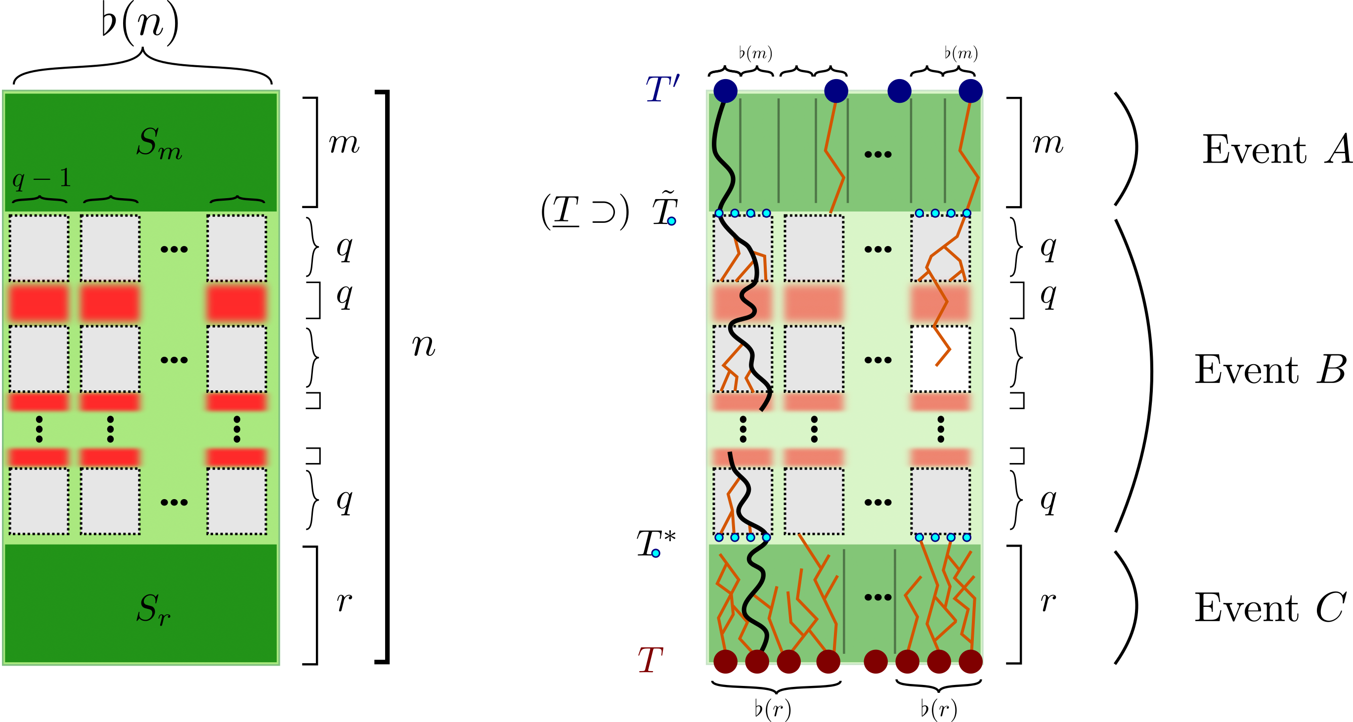
Figure 11: Drilling/generating a crossing of $S$. The Events $A,B,C$ together yield the crossing (bold black path) with a minimal probability depending on $\#T^{\prime}$.

In Lemma 50, we pool together small strips and estimate the probability of a crossing happening for at least one of them. Then, we estimate the probability of Event $A$ in Lemma 51. We do so by pooling several $(m,\flat(m))$ strips together so that each such collection has a sufficiently high probability of crossing $S_{m}$. Lemma 50 allows us to pool together all survivors from Event $A$ to obtain a lower bound on the probability of Event $C$. Finally, Proposition 48 follows from combining all of the previous calculations.

Let us briefly consider a general $(j,J)$ strip $S^{*}$ with $j<n$ and $J\geq\flat(j)$. Let $\hat{S}:=\cup\hat{S}_{i}$ be a disjoint union of $(j,\flat(j))$ strips in $S^{*}$. Let $T^{*}$ (the target) be a $(\kappa[\shortparallel],J)$-tree on the bottom of $S^{*}$ which intersects each $\hat{S}_{i}$ in a $(\kappa[\shortparallel],\flat(j))$-tree. Let $\hat{T}$ be a union of $l$-trees on top of $\hat{S}$ where $l\leq\flat(j)$, all lying in the columns of $T^{*}$.

Lemma 50 (Pooling together strips for crossings, [Hof05, Lemma 4.4]).

Suppose Proposition 48 holds for $j\leq n-2$. Then,

$$\mathbb{P}(\exists\text{ a crossing of }\hat{S}\text{ intersecting }\hat{T}\text{ and }T^{*} )\geq\min\left\{0.9,\,\tfrac{1}{3}\kappa[\shortparallel]^{\flat(j)}\cdot\#\hat{T}\right\}\,.$$

Each such crossing is confined to its respective $(j,\flat(j))$ strip.

Proof.

$\hat{T}$ is a union of $(\kappa[\shortparallel],l)$ trees. Let $\hat{T}=\cup\hat{T}_{i}$ where $\hat{T}_{i}$ consists of the $(\kappa[\shortparallel],l)$ trees belonging to $\hat{T}$ that lie inside the $(j,\flat(j))$ strip $\hat{S}_{i}$ (recall $l\leq\flat(j)$). By the induction hypothesis, we have

$$\mathbb{P}(\exists\text{ a crossing of }\hat{S_{i}}\text{ intersecting }\hat{T_{i}}\text{ and }T^{*})\geq\kappa[\shortparallel]^{-\flat(j)}\cdot\#\hat{T_{i}}\,.$$

These are independent events since all the $\hat{S}_{i}$ are disjoint. Lemma 49 with $c=2.31$ yields

$$\mathbb{P}(\exists\text{ a crossing of } \hat{S}\text{ intersecting }\hat{T}\text{ and }T^{*})$$

$$\geq 1-\prod_{i}\big{(}1-\mathbb{P}\{\exists\text{ a crossing of }\hat{S_{i}}\text{ intersecting }\hat{T_{i}}\text{ and }T^{*}\}\big{)}$$

$$\geq(1-e^{-2.31})\min\Big{\{}1,\,\tfrac{1}{2.31}\kappa[\shortparallel]^{-\flat(j)}\sum_{i}\#\hat{T}_{i}\Big{\}}\geq\min\left\{0.9,\,\tfrac{1}{3}\kappa[\shortparallel]^{-\flat(j)}\cdot\#\hat{T}\right\}$$

which shows the claim. Furthermore, the crossing happens in one of the $\hat{S}_{i}$. ∎

Let us return to our $(n,\flat(n))$ strip $S$. On the bottom of it, there is a target $(\kappa[\shortparallel],\flat(n))$ tree $T$, while on top of it, there is a union of $(\kappa[\shortparallel],k)$ trees $T^{\prime}$ with $\pi_{x}(T^{\prime})\subset\pi_{x}(T)$. We also recall the parameters $q,m$ and $k$. Let

$$M:=\max\left\{\flat(m),\,q-1\right\}\qquad k^{\prime}:=\min\left\{k,\,\flat(m)\right\} \,.$$

and $\underline{T}$ be a $(\kappa[\shortparallel],\flat(n))$ tree on the bottom of $S_{m}$ with $\pi_{x}(\underline{T})=\pi_{x}(T)$. This tree will act as the target for the survivors of Event $A$. Next, we have to count the survivors.

Define $\tilde{T}$ to be the union of $(\kappa[\shortparallel],q-1)$ trees in $\underline{T}$ satisfying the following: Let $\tilde{T}_{i}$ be a $(\kappa[\shortparallel],q-1)$ tree inside a $(m,M)$ strip. Then $\tilde{T}_{i}\subset\tilde{T}$ if there are $v_{i}^{\prime}\in T^{\prime}$ and $\tilde{v}_{i}\in\tilde{T}_{i}$ such that $v_{i}^{\prime}\leadsto\tilde{v}_{i}$ inside $S_{m}$. Define the event

$$\mathfrak{X}:=\Big{\{}\#\tilde{T}\geq\max\big{\{}\frac{\kappa[\shortparallel]^{q-2}\cdot\#T^{\prime}}{8\cdot\kappa[\shortparallel]^{M}},\,\kappa[\shortparallel]^{q-2}\big{\}}\Big{\}}\,.$$ (12)

Remark (On $M,k^{\prime}$).

We have to consider $(m,M)$ strips rather than $(m,\flat(m))$ strips because multiple $(m,\flat(m))$ strips might connect to the same $q-1$ box in the case of $q-1>\flat(m)$. This would result in double counting for $\tilde{T}$. On the other hand, introducing $k^{\prime}$ basically just means that we break up $(\kappa[\shortparallel],k)$ trees into smaller $(\kappa[\shortparallel],k^{\prime})=(\kappa[\shortparallel],\flat(m))$ trees so that they act as proper inputs for the $(m,\flat(m))$ strips.

We only count hits of $(\kappa[\shortparallel],q-1)$ trees since each (single) connection will yield a full tree after passing through a $q-1$ box (or rather a $q-1$ column in Event B later).

Lemma 51 (Probability of “sufficiently many” crossings, [Hof05, Lemma 4.5]).

Suppose Proposition 48 holds for $j\leq n-2$. Then

$$\mathbb{P}(\mathfrak{X})\geq\min\left\{0.9,\,\tfrac{1}{8}\kappa[\shortparallel]^{-\flat(m)}\cdot\#T^{\prime}\right\}\,.$$

Proof.

Since $\tilde{T}$ consists of $(\kappa[\shortparallel],q-1)$ trees and each such tree has $\kappa[\shortparallel]^{q-2}$ many vertices, we have $\#\tilde{T}\geq\kappa[\shortparallel]^{q-2}$ if and only if $\tilde{T}\neq\emptyset$. In order to show $\#\tilde{T}\geq\kappa[\shortparallel]^{q-2}$, it therefore suffices to show $T^{\prime}\leadsto\underline{T}$. The proof is broken up into cases based on the size of $\#T^{\prime}$ and the value of $M$.

1. $\#T^{\prime}\leq 8\cdot\kappa[\shortparallel]^{\flat(m)}$ and $M=\flat(m)$. In particular, $\flat(m)\geq q-1$. Therefore, by Lemma 50 with $S^{\prime}=S_{m}$, $\hat{S}$ to be a union of $(m,\flat(m))$ strips, $T^{*}=\underline{T}$ and $\hat{T}=T^{\prime}$

   $$\mathbb{P}(\mathfrak{X})=\mathbb{P}(\#\tilde{T}\geq\kappa[\shortparallel]^{q-2})\geq\mathbb{P}(\exists\text{ a crossing }T^{\prime}\leadsto\underline{T}\text{ inside }S_{m})\geq\min\Big{\{}0.9,\,\tfrac{1}{3}\kappa[\shortparallel]^{-\flat(m)}\cdot\#T^{\prime}\Big{\}}\,.$$

2. $\#T^{\prime}\leq 8\cdot\kappa[\shortparallel]^{M}$ and $M=q-1$. Again

   $$\mathbb{P}(\mathfrak{X})=\mathbb{P}(\#\tilde{T}\geq\kappa[\shortparallel]^{M-1})=\mathbb{P}(\#\tilde{T}\geq\kappa[\shortparallel]^{q-2})\,.$$

   Write $T^{\prime}=\cup_{i=1}^{N}T_{i}$ where each $T_{i}$ is a union of $(\kappa,k^{\prime})$ trees in a $(m,\flat(m))$ strip. Then, for all $i$ by Lemma 50

   $$\mathbb{P}\big{\{}T_{i}\leadsto\underline{T}\text{ inside a }(m,\flat(m))\text{ strip}\big{\}}\geq\min\left\{0.9,\,\tfrac{1}{3}\kappa[\shortparallel]^{-\flat(m)}\cdot\#T_{i}\right\}\,.$$

   We are done if the minimum for one of the $i$ is $0.9$. Otherwise, Lemma 50 concludes

   $$\mathbb{P}\big{\{}T^{\prime}\leadsto\underline{T}\text{ inside some }(m,\flat(m))\text{ strip}\big{\}}\geq\min\left\{0.9,\,\tfrac{1}{3}\kappa[\shortparallel]^{-\flat(m)}\cdot\#T^{\prime}\right\}\,.$$

3. $\#T^{\prime}>8\cdot\kappa[\shortparallel]^{M}$. This is the case where we actually have to establish multiple crossings in disjoint regions. Write $T^{\prime}=\cup_{i=1}^{N^{\prime}}T_{i}^{\prime}$ where each $T_{i}^{\prime}$ is now a union of $k^{\prime}$ trees that belong to a union of $(m,M)$ strips $\tilde{S}_{i}$. Do this in a way such that for each $i$

   $$3\cdot\kappa[\shortparallel]^{M}\leq\#T^{\prime}_{i}\leq 4\cdot\kappa[\shortparallel]^{M}$$

   and such that if $i\neq j$, then the corresponding unions of $(m,M)$ strips $\tilde{S}_{i}$ and $\tilde{S}_{j}$ are disjoint. This is possible since each $k^{\prime}$ tree has $\kappa[\shortparallel]^{k^{\prime}-1}$ vertices and $M\geq\flat(m)\geq k^{\prime}$. Thus, $N^{\prime}$ satisfies

   $$N^{\prime}\geq\frac{\#T^{\prime}}{4\cdot\kappa[\shortparallel]^{M}}\geq\frac{8\cdot\kappa[\shortparallel]^{M}}{4\cdot\kappa[\shortparallel]^{M}}=2\,.$$

   By Lemma 50, we have with $\#T_{i}^{\prime}\geq 3\cdot\kappa[\shortparallel]^{M}$

   $$\mathbb{P}\big{\{}T_{i}^{\prime}\leadsto\bar{T}\text{ inside some }(m,M)\text{ strip}\big{\}}\geq\min\left\{0.9,\,\tfrac{1}{3}\kappa[\shortparallel]^{-\flat(m)}\cdot\#T_{i}^{\prime}\right\}=0.9\,.$$

   Therefore, we have $N^{\prime}$ independent events with probability greater or equal to $0.9$. The probability of at least $\lceil N^{\prime}/2\rceil$ of these happening is $\geq 0.9$. Each such event gives us a contribution of $\kappa[\shortparallel]^{q-2}$ to $\#\tilde{T}$, so we see that under the event of at least $\lceil N^{\prime}/2\rceil$ crossings happening

   $$\#\tilde{T}\geq\frac{N^{\prime}}{2}\cdot\kappa[\shortparallel]^{q-2}\geq\frac{\#T^{\prime}\cdot\kappa[\shortparallel]^{q-2}}{8\cdot\kappa[\shortparallel]^{M}}\,.$$

   Therefore

   $$\mathbb{P}(\mathfrak{X})\geq\mathbb{P}\Big{(}\#\tilde{T}\geq\frac{\#T^{\prime}\cdot\kappa[\shortparallel]^{q-2}}{8\cdot\kappa[\shortparallel]^{M}}\Big{)}\geq 0.9=\min\left\{0.9,\,\tfrac{1}{8}\kappa[\shortparallel]^{-\flat(m)}\cdot\#T^{\prime}\right\}\,.$$

With this, all cases have been covered. ∎

This covers event $A$. Next up is event $B$. Take a column of $q-1$ boxes including the $(q,q-1)$ strips inbetween. Let us fix a survivor $v\in\underline{T}$ from Event $A$, that is, $v$ satisfies $T^{\prime}\leadsto v$. We now formalise what is meant by event $B$:

Definition 52 (Good $q-1$ columns ).

Let a column of up to $12\mathfrak{s}_{t}$ many $q-1$ boxes be given including their $(q,q-1)$ strips inbetween. We call it a $q-1$ column and we call it good for $v,w\in G$ if $v\leadsto w$ inside $G$.

Lemma 53 (Probability of good $q-1$ columns [Hof05, Lemma 4.6]).

Suppose Lemma 24 holds for $q-1\leq n-2$. Consider a $q-1$ column $G$ and $v,w\in G$ where $v$ is a a vertex on the top and $w$ on the bottom of $G$. Then,

$$\mathbb{P}(G\text{ is good for }v,w)\geq 0.99\,.$$

Proof.

First, we see that $G$ is good for $v$ and $w$ if

1. all the corresponding $q-1$ boxes and $(q,q-1)$ strips are good and

2. $v\in\mathtt{In}(\bar{B}_{q-1})$ with $\bar{B}_{q-1}$ being the topmost $q-1$ box in $G$.

3. $w\in\mathtt{Out}(\underline{B}_{q-1})$ with $\underline{B}_{q-1}$ being the bottommost $q-1$ box in $G$.

By the induction hypothesis

$$\mathbb{P}(\text{all of the }q-1\text{ boxes are good})\geq(1-\mathbbm{p})^{12\mathfrak{s}_{t}}\geq 1-12\mathfrak{s}_{t}\cdot\mathbbm{p}\,,$$

and

$$\mathbb{P}(\text{all of the }(q,q-1)\text{ strips are good})\geq(1-\mathbbm{p})^{12\mathfrak{s}_{t}}\geq 1-12\mathfrak{s}_{t}\cdot\mathbbm{p}\,.$$

Next, $v\in\mathtt{In}(\bar{B}_{q-1})$ if $v$ lies in good $j$ boxes for all $j\leq q-1$. The probability of this happening is at least

$$\mathbb{P}(v\in\mathtt{In}(\bar{B}_{q-1}))\geq 1-\sum_{j\geq 1}\mathbbm{p}^{j}=\frac{1-2\mathbbm{p}}{1-\mathbbm{p}}\geq 1-2\mathbbm{p}\,.$$

The same holds for $w$. Using $\mathbbm{p}\leq(450\mathfrak{s}_{t}\cdot\mathfrak{s}_{x})^{-6}$ yields

$$\mathbb{P}(G\text{ is good for }v,w)\geq 1-25\mathfrak{s}_{t}\cdot\mathbbm{p}\geq 0.99\,,$$

which finishes the proof. ∎

Event $C$ corresponds to Lemma 50.

4.5 Drilling: proof of Proposition 48

We have gathered all the parts, so it is time to combine them. Unfortunately, we have to deal with quite a lot of case distinctions.

Proof of Proposition 48.

We have already shown the case of $q\leq 2$ which also includes the case of $\min\{m,r\}\leq 3$. Now, we may always assume that $m\geq 4$ as well as $q\geq 3$.We employ our strategy of linking together the Events $A$, $B$ and $C$, that is,

1. $\mathfrak{X}$ happens on $S_{1}$. This gives us a collection of $(\kappa[\shortparallel],q-1)$ trees $\tilde{T}\subset\bar{T}$ on the bottom of $S_{m}$. Each such tree has some $v\in\tilde{T}$ with $T^{\prime}\leadsto v$.

2. Consider $T^{*}$ on the top of $S_{r}$ with $\pi_{x}(\tilde{T})=\pi_{x}(T^{*})$. There exists a crossing of $S_{2}$ intersecting $T^{*}$ and $T$, i.e., some $T^{*}\ni w\leadsto T$.

3. The $q-1$ column of $w\in T^{*},v[w]\in\tilde{T}$ is good.

If all these events hold, then there exists a crossing of $S$ from $T^{\prime}$ to $T^{\prime}$ via

$$T^{\prime}\leadsto^{A}\tilde{T}\ni v[w]\leadsto^{B}w\in T^{*}\leadsto^{C}T\,.$$

By Lemma 51

$$\mathbb{P}(A)=\mathbb{P}(\mathfrak{X})\geq\min\left\{0.9,\,\tfrac{1}{8}\kappa[\shortparallel]^{-\flat(m)}\#T^{\prime}\right\}\,.$$

Under $\mathfrak{X}$, we have

$$\#\tilde{T}\geq\max\left\{\kappa[\shortparallel]^{q-2},\,\frac{\kappa[\shortparallel]^{q-2}\cdot\#T^{\prime}}{8\cdot\kappa[\shortparallel]^{M}}\right\}\,.$$

• If now $\#T^{\prime}\leq 8\cdot\kappa[\shortparallel]^{M}$ , then $\#T^{*}=\#\tilde{T}\geq\kappa[\shortparallel]^{q-2}$ and by the Lemmas 51, 53

  $$\mathbb{P}(B,C\,|\,A) \geq\mathbb{P}(\exists\text{ a crossing of }S_{2}\text{ intersecting }T^{*}\text{ and }T\,|\,\#T^{*}=\kappa[\shortparallel]^{q-2})\cdot 0.99$$

  $$\geq 0.99\cdot\min\left\{0.9,\,\tfrac{1}{3}\kappa[\shortparallel]^{-\flat(r)}\kappa[\shortparallel]^{q-2}\right\}\,.$$

  If $M=\flat(m)$, then using Equation (13) from Lemma 54 below yields

  $$\mathbb{P}(\exists\text{ a cluster in }S \text{ connecting }T\text{ and }T^{\prime})\geq\mathbb{P}(A)\cdot\mathbb{P}(B,C\,|\,A)$$

  $$\geq 0.9\cdot\tfrac{1}{8}\kappa[\shortparallel]^{-\flat(m)}\#T^{\prime}\,\cdot\,0.99\cdot\min\left\{0.9,\,\tfrac{1}{3}\kappa[\shortparallel]^{-\flat(r)}\kappa[\shortparallel]^{q-2}\right\}$$

  $$\geq \#T^{\prime}\cdot\tfrac{1}{27}\kappa[\shortparallel]^{-\flat(n)+\lfloor q/2\rfloor}\geq\kappa[\shortparallel]^{-\flat(n)}\cdot\#T^{\prime}\,.$$

  For the case of $M=q-1$, i.e. $8\cdot\kappa[\shortparallel]^{\flat(m)}\leq\#T^{\prime}\leq 8\cdot\kappa[\shortparallel]^{M}$, using Equation (13) of Lemma 54 and $\flat(m)>m/2\geq\lceil q/2\rceil$ yields

  $$\mathbb{P}(\exists \text{ a cluster in }S\text{ connecting }T\text{ and }T^{\prime})\geq\mathbb{P}(A)\cdot\mathbb{P}(B,C\,|\,A)$$

  $$\geq 0.9\,\cdot\,0.99\cdot\min\left\{0.9,\,\tfrac{1}{3}\kappa[\shortparallel]^{q-2-\flat(r)}\right\}\geq\min\left\{0.5,\,\tfrac{1}{4}\frac{\kappa[\shortparallel]^{M-1}\cdot\kappa[\shortparallel]^{\flat(m)}}{\kappa[\shortparallel]^{\flat(m)+\flat(r)}}\right\}$$

  $$\geq \min\left\{0.5,\,\tfrac{1}{4}\frac{\kappa[\shortparallel]^{M-1}\cdot\kappa[\shortparallel]^{\lceil q/2\rceil}}{\kappa[\shortparallel]^{\flat(n)-\lceil q/2\rceil-2}}\right\}\geq\min\left\{0.5,\,\frac{\kappa[\shortparallel]^{M}\cdot 8}{\kappa[\shortparallel]^{\flat(n)}}\right\}\geq\frac{\#T^{\prime}}{\kappa[\shortparallel]^{\flat(n)}}\,.$$

• If instead $\#T^{\prime}\geq 8\cdot\kappa[\shortparallel]^{M}$, then using

  $$\#\tilde{T}=\#T^{*}\geq\frac{\#T^{\prime}\cdot\kappa[\shortparallel]^{q-2}}{8\cdot\kappa[\shortparallel]^{M}}$$

  and Lemma 50 and Equation (14) gives

  $$\mathbb{P}(C\,|\,A) \geq\mathbb{P}\Big{\{}\exists\text{ a crossing of }S_{2}\text{ intersecting }T^{*}\text{ and }T\,|\,\#T^{*}\geq\frac{\#T^{\prime}\cdot\kappa[\shortparallel]^{q-2}}{8\cdot\kappa[\shortparallel]^{M}}\Big{\}}$$

  $$\geq\min\left\{0.9,\,\frac{\#T^{\prime}\cdot\kappa[\shortparallel]^{q-2}}{8\cdot\kappa[\shortparallel]^{M}}\cdot\frac{1}{3\cdot\kappa[\shortparallel]^{\flat(r)}}\right\}\geq\min\left\{0.9,\,\frac{\#T^{\prime}}{24\cdot\kappa[\shortparallel]^{\flat(n)-1}}\right\}\geq 2\frac{\#T^{\prime}}{\kappa[\shortparallel]^{\flat(n)}}\,,$$

  where the minimum disappears again from $\#T^{\prime}\leq\#T\leq\kappa[\shortparallel]^{\flat(n)-1}$. Lemma 53 yields

  $$\mathbb{P}(B\,|\,A,C)\geq 0.99\,.$$

  Putting everything together, we conclude the $\#T^{\prime}\geq 8\cdot\kappa[\shortparallel]^{M}$ case:

  $$\mathbb{P}(\exists\text{ a cluster in } S\text{ connecting }T\text{ and }T^{\prime})\geq\mathbb{P}(A)\cdot\mathbb{P}(C\,|\,A)\cdot\mathbb{P}(B\,|\,A,C)$$

  $$\geq 0.9\cdot 2\cdot\frac{\#T^{\prime}}{\kappa[\shortparallel]^{\flat(n)}}\cdot 0.99\geq\frac{\#T^{\prime}}{\kappa[\shortparallel]^{\flat(n)}}\,.$$

This finishes the proof of Proposition 48. ∎

Lemma 54 (Extra estimates for final proof).

Let $m\geq 4,q\geq 3$ and $M=\max(\flat(m),q-1)$. We have

$$\flat(m)+\flat(r)-\lceil q/2\rceil\leq\flat(n)-2\,.$$ (13)

Furthermore, we have

$$M+\flat(r)-q \leq\flat(n)-3\,.$$ (14)

Proof.

If $3\leq q\leq 8$, then $m+r=n$ by Equation (6) in Lemma 40. In particular,

$$\flat(m)+\flat(r)\leq\flat(n)\implies\flat(m)+\flat(r)-\lceil q/2\rceil\leq\flat(n)-2\,.$$

If $q\geq 9$, then we use

$$\lceil(2-\mathfrak{d})^{-1}(\lfloor\mathfrak{d}q\rfloor+1)\rceil\leq q/21+2\leq\lceil q/2\rceil-2$$

to also obtain Equation (13) via Equation (7) in Lemma 40

$$m+r-\lfloor\mathfrak{d}q\rfloor \leq n+1$$

$$\flat(m)+\flat(r)-\lceil(2-\mathfrak{d})^{-1}(\lfloor\mathfrak{d}q\rfloor+1)\rceil \leq\flat(n)$$

$$\flat(m)+\flat(r)-\lceil q/2\rceil \leq\flat(n)-2\,.$$

For Equation (14), we need another case distinction: If $M=\flat(m)$, then

$$M+\flat(r)-q =\big{\{}\flat(m)+\flat(r)-\lfloor q/2\rfloor\big{\}}-\lceil q/2\rceil\leq\flat(n)-2-1$$

Else, we have $M=q-1$, which yields

$$M+\flat(r)-q =\flat(r)-1=\flat(n)-2-\big{\{}\flat(m)-\lfloor q/2\rfloor\big{\}}\,.$$

Since $\flat(m)>m/2>\lfloor(m-1)/2\rfloor\geq\lfloor q/2\rfloor$ and $M+\flat(r)-q$ is an integer, this case also implies $M+\flat(r)-q\leq\flat(n)-3$, i.e., Equation (14). ∎

Acknowledgement. This work was supported by the German Research Foundation under Germany’s Excellence Strategy MATH+: The Berlin Mathematics Research Center, EXC-2046/1 project ID: 390685689, and the Leibniz Association within the Leibniz Junior Research Group on Probabilistic Methods for Dynamic Communication Networks as part of the Leibniz Competition.

References

- [BDS91] M. Bramson, R. Durrett and R.H. Schonmann “The contact process in a random environment” In The Annals of Probability 19.3, 1991, pp. 960–983
- [BH57] S.R. Broadbent and J.M. Hammersley “Percolation processes. I. Crystals and mazes” In Proceedings of the Cambridge Philosophical Society 53, 1957, pp. 629–641
- [Dur84] R. Durrett “Oriented percolation in two dimensions” In The Annals of Probability 12.4, 1984, pp. 999–1040
- [Fon+23] L.R. Fontes, T.S. Mountford, D. Ungaretti and M.E. Vares “Renewal contact processes: phase transition and survival” In Stochastic Processes and their Applications 161, 2023, pp. 102–136
- [GH02] G. Grimmett and P. Hiemer “Directed percolation and random walk” In In and out of equilibrium (Mambucaba, 2000) 51, Progr. Probab. Birkhäuser Boston, Boston, MA, 2002, pp. 273–297
- [GL22] P.A. Gomes and B.N.B. Lima “Long-range contact process and percolation on a random lattice” In Stochastic Processes and their Applications 153, 2022, pp. 21–38
- [Har74] T.E. Harris “Contact interactions on a lattice” In The Annals of Probability 2, 1974, pp. 969–988
- [Hil+22] M. Hilário, D. Ungaretti, D. Valesin and M.E. Vares “Results on the contact process with dynamic edges or under renewals” In Electronic Journal of Probability 27, 2022, pp. Paper No. 91\bibrangessep31
- [Hil+23] M.R. Hilário, M. Sá, R. Sanchis and A. Teixeira “Phase transition for percolation on a randomly stretched square lattice” In The Annals of Applied Probability 33.4, 2023, pp. 3145–3168
- [Hof05] C. Hoffman “Phase transition in dependent percolation” In Communications in Mathematical Physics 254, 2005, pp. 1–22
- [JJV23] B. Jahnel, S.K. Jhawar and A.D. Vu “Continuum Percolation in a Nonstabilizing Environment” In Electronic Journal of Probability (accepted) arXiv:2205.15366, 2023
- [Kes80] H. Kesten “The critical probability of bond percolation on the square lattice equals ” In Communications in Mathematical Physics 74.1, 1980, pp. 41–59
- [KSV22] H. Kesten, V. Sidoravicius and M.E. Vares “Oriented percolation in a random environment” In Electronic Journal of Probability 27, 2022, pp. Paper No. 82\bibrangessep49
- [LS23] J.N. Latz and J.M. Swart “Applying monoid duality to a double contact process” In Electronic Journal of Probability 28, 2023, pp. Paper No. 70\bibrangessep26
- [LSV23] B.N.B. Lima, V. Sidoravicius and M.E. Vares “Dependent percolation on ” In Brazilian Journal of Probability and Statistics 37.2, 2023, pp. 431–454
- [RV22] B. Ráth and D.l Valesin “On the threshold of spread-out contact process percolation” In Annales de l’Institut Henri Poincaré Probabilités et Statistiques 58.3, 2022, pp. 1808–1848
- [SS23] M. Seiler and A. Sturm “Contact process in an evolving random environment” In Electronic Journal of Probability 28, 2023, pp. Paper No. 1