Random resetting in search problems

Abstract

By periodically returning a search process to a known or random state, random resetting possesses the potential to unveil new trajectories, sidestep potential obstacles, and consequently enhance the efficiency of locating desired targets. In this chapter, we highlight the pivotal theoretical contributions that have enriched our understanding of random resetting within an abundance of stochastic processes, ranging from standard diffusion to its fractional counterpart. We also touch upon the general criteria required for resetting to improve the search process, particularly when distribution describing the time needed to reach the target is broader compared to a normal one. Building on this foundation, we delve into real-world applications where resetting optimizes the efficiency of reaching the desired outcome, spanning topics from home range search, ion transport to the intricate dynamics of income. Conclusively, the results presented in this chapter offer a cohesive perspective on the multifaceted influence of random resetting across diverse fields.

1 Introduction

When in doubt, reset!

Random resetting is a concept that has gained substantial attention in recent years as a novel and counter-intuitive approach to solving complex search problems. This technique has provided groundbreaking insights into the stochastic nature of search processes whose behavior can often confound traditional models and approaches evans2020stochastic . In this chapter, we delve into the fascinating interplay between random resetting and search processes. We explore how resetting randomly to a new location evans2020stochastic ; evans2011diffusion ; pal2015diffusion ; evans2013optimal ; eule2016non ; nagar2016diffusion ; mendez2016characterization ; kumar2023universal ; kusmierz2014first ; bonomo2021first ; belan2018restart acts as a mechanism that provides new insights into the dynamics of various stochastic systems, enhancing our ability to predict and control their behavior.

But why would random resetting improve the modeling of search processes?

By periodically returning the search process to a known or random state, random resetting uncovers new pathways, avoids potential pitfalls, and can lead to an unexpected efficiency in reaching desired targets evans2011diffusion ; evans2011diffusionJPA ; evans2020stochastic ; pal2017first ; reuveni2016optimal ; chechkin2018random . Consider home range search, a realm where the influence of random resetting has yielded unprecedented advances in efficiency and understanding pal2020search ; tal2020experimental ; besga2020optimal . In ecological studies, animals often search within a specific home range to find food, mates, or shelter. Traditional models may struggle to accurately represent the stochastic nature of this behavior. The introduction of random resetting, where the search is periodically returned to the “home” of the searcher or a random state, helps model the realistic unpredictability of search patterns within an animal’s home range (see Fig. 1). This approach not only simulates the dynamic interplay between an animal’s instinctive behavior and random environmental factors, leading to more accurate representations, but also reveals that search with home returns can outperform free-range search, particularly in conditions of high uncertainty pal2020search .

Now consider the field of economics, specifically in the modeling of individual income dynamics, where random resetting introduces a vital perspective stojkoski2022income ; gabaix2016dynamics ; vinod2022nonergodicity . Understanding the time needed for an individual to improve their income is crucial for various economic decisions, from personal financial planning to governmental policy-making jolakoski2023first . Traditional models, however, may overlook the complex and often abrupt changes in an individual’s financial situation, such as losing a job or retirement. By incorporating random resetting, which can mimic these sudden transitions, economists are provided with a more realistic portrayal of the time dynamics involved in income improvement. This approach not only offers a nuanced depiction of income trajectories but also recognizes the stabilizing effect of these “reset” points, acknowledging their real-world relevance.

But the application of random resetting in search problems goes way beyond these two examples. From the intricate pathways of cellular biology boyer2014random ; roldan2016stochastic ; ramoso2020stochastic ; budnar2019anillin , chemical reactions reuveni2014role ; rotbart2015michaelis ; biswas2023rate ; budnar2019anillin , foraging pal2020search ; moran2023modeling ; benichou2011intermittent , nonlinear dynamical systems ray2021mitigating , operation research bonomo2022mitigating to computer algorithms luby1993optimal ; blumer2022stochastic , the principles of random resetting continue to offer fresh insights and innovative solutions. The versatility and adaptability of this concept have allowed researchers and practitioners to tackle previously intractable challenges, forging connections between disparate fields and creating a cohesive understanding of the underlying dynamics of search processes.

In this chapter, we systematically explore the multifaceted realm of search processes with random resetting. In Section 2, we introduce a robust mathematical framework, elucidating the core concepts and recent advancements that have shaped our understanding of search under the influence of random resetting. Moving forward, in Section 3, we delve into examples of search processes under resetting, offering a detailed examination of the intriguing theoretical behaviors and patterns that arise from the interplay between search strategies and random resets. This includes a focus on how random resetting can influence metrics such as first passage time. Next, in Section 4, we explore the delicate balance between too much and too little resetting, investigating strategies that maximize efficiency in search processes by optimizing the resetting rate. Then, in Section 5, we showcase diverse applications of search processes under random resetting, demonstrating the wide-ranging impact of this approach on contemporary science and technology, as well as its practical solutions to real-world challenges. Finally, we synthesize the insights gleaned from our exploration, highlighting both the theoretical underpinnings and practical implications of incorporating random resetting into search processes.

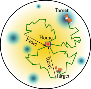
Figure 1: Schematic for a stochastic search process under resetting in a confined topography in the presence of multiple targets (dark green circles). The searcher (e.g., a prairie fox) looks for targets (which can be food, companion or other resources) in the vicinity of its home and intermittently returns there to take rest. Following this spatial reset, the searcher resumes its search, more likely wandering to a different direction. The search is completed after it has found one or multiple targets in the domain. The central aim here is to understand the behavior of the mean search time under random resetting, in particular, as a function of the frequency of resetting or return.

2 The renewal formalism for first passage under resetting

In this section, we discuss the first passage properties of a resetting process. Let us consider a generic search process conducted by a stochastic searcher $\vec{x}(t)$ in an arbitrary domain $\mathcal{D}$ in the presence of a single or multiple targets. The initial condition of the process is assumed to be $\vec{x}(0)=\vec{x_{0}}$. The process is completed when the searcher finds one of these targets and one would be interested in the statistics of the stochastic search time $T$, distribution of which is denoted by the first passage time density $f_{T}(t|\vec{x_{0}})$. It is often useful to introduce $Q_{0}(t|\vec{x_{0}})$ that defines the survival probability of the underlying process that it has not found any target until time $t$, starting from the initial configuration $\vec{x_{0}}$. Clearly, this quantity is related to the position distribution function, denoted by $P_{0}(\vec{x},t|\vec{x_{0}},0)$, of the searcher in the following way $Q_{0}(t|\vec{x_{0}})=\int_{\mathcal{D}}~{}d\vec{x}P_{0}(\vec{x},t|\vec{x_{0}},0)$. In the absence of targets, the searcher always survives thus $Q_{0}(t|\vec{x_{0}})=1$, otherwise it decays to zero in large time as the searcher eventually finds the target. In other words, the search process is completed.

To introduce resetting, let us consider that the underlying first passage process is intermittently stopped and restarted from some pre-selected configuration. Simply put, after each resetting event, the searcher goes back to a fixed location $\vec{x_{R}}$ or locations drawn from an identical ensemble $P(\vec{x_{R}})$. The waiting times between the resetting events are drawn from a normalized density $f_{R}(t)$. Under this mechanism, the new first passage time is denoted by $T_{r}$ which will be distributed via the first passage time density $f_{T_{r}}(t|\vec{x_{0}})$. The subscript ‘$r$’ is used to indicate the presence of resetting events. Here, $Q_{r}(t|\vec{x_{0}};\vec{x_{R}})$ denotes the survival probability in the presence of resetting. In words, this measures the probability to find the searcher inside the domain $\mathcal{D}$ upto time $t$ given that it had started at $\vec{x_{0}}$ at time zero and experienced multiple resetting to $\vec{x_{R}}$. In this chapter, we assume that the waiting times between resetting are drawn from $f_{R}(t)=re^{-rt}$ which essentially means that resetting occurs at a rate $r$.

Since each resetting event compels the searcher to start from scratch, the first passage process under resetting generically belongs to the broad class of stochastic renewal processes. Adapting the mathematical structure from there, one can write a renewal equation for the survival probability $Q_{r}(t|\vec{x_{0}};\vec{x_{R}})$ in the following way evans2011diffusion ; evans2020stochastic

$$Q_{r}(t|\vec{x_{0}};\vec{x_{R}})=e^{-rt}Q_{0}(t|\vec{x_{0}})+r\int_{0}^{t}d\tau_{l}e^{-r\tau_{l}}Q_{0}(\tau_{l}|\vec{x_{R}})Q_{r}(t-\tau_{l}|\vec{x_{0}};\vec{x_{R}})~{}.$$ (1)

Eq. 1 has a simple interpretation. The first term on the right hand side implies that the particle survives till time $t$ without experiencing any reset event. The second term considers the possibility when there are multiple reset events. One can then look at a long trajectory where the last reset event had occurred at time $t-\tau_{l}$, and after that there has been no reset for the duration $\tau_{l}$. This probability is given by $rd\tau_{l}e^{-r\tau_{l}}$. But then this has to be multiplied by $Q_{r}(t-\tau_{l}|\vec{x_{0}};\vec{x_{R}})$, i.e., the probability that the particle survives till time $t-\tau_{l}$ with multiple reset events and $Q_{0}(\tau_{l}|\vec{x_{R}})$, i.e., the survival probability of the particle for the last non-resetting interval $\tau_{l}$, starting from $\vec{x_{R}}$. This is a useful formula since the survival properties for the resetting process can be directly understood from the reset-free processes. Notably, the construction of the above equation relied upon the last resetting event, hence this approach is often known as the last renewal formalism. Similar to this, a first renewal formalism can also be developed for the survival probability. The corresponding renewal equation reads pal2016diffusion

$$Q_{r}(t|\vec{x_{0}};\vec{x_{R}})=e^{-rt}Q_{0}(t|\vec{x_{0}})+r\int_{0}^{t}d\tau_{f}e^{-r\tau_{f}}Q_{0}(\tau_{f}|\vec{x_{0}})Q_{r}(t-\tau_{f}|\vec{x_{R}};\vec{x_{R}})~{},$$ (2)

where we assume that the first resetting occurs at time $\tau_{f}$, and upto that there was no resetting (with the probability $e^{-r\tau_{f}}$). Until then the particle survives with $Q_{0}(\tau_{f}|\vec{x_{0}})$ – the reset free survival probability. For the rest time interval $t-\tau_{f}$, the particle survives with many resetting events – the probability of which is assigned by $Q_{r}(t-\tau_{f}|\vec{x_{R}};\vec{x_{R}})$. It is easy to see that both (1) and (2) are identical (see evans2020stochastic ; pal2016diffusion ). Notably, the renewal formalism does not require any particular choice of the underlying dynamics i.e., the renewal equations hold both for the Markovian and the non-Markovian anomalous search processes. The only key assumption here is that no memory of the dynamics can be carried forward from one interval to the next. Crucially, as we show below, that it is not required to have the expression for the survival probability $Q_{0}(t|\cdot)$ of the underlying process in the real time domain - remarkably, an expression in the Laplace space is sufficient to extract further information. To see this, let us apply the Laplace transform on the both sides of Eq. (1) which satisfies

$$\widetilde{Q_{r}}(s|\vec{x_{0}};\vec{x_{R}})=\frac{\widetilde{Q_{0}}(s+r|\vec{x_{0}})}{1-r\widetilde{Q_{0}}(s+r|\vec{x_{R}})}~{},$$ (3)

where $\widetilde{\mathcal{G}}(s)=\mathscr{L}_{t\to s}\left[\mathcal{G}(t)\right]$ is the Laplace transform of the function $\mathcal{G}(t)$. The first passage time density $f_{T_{r}}(t|\vec{x_{0}})$ is the negative gradient of the survival probability in time such that redner2001guide ; bray2013persistence

$$f_{T_{r}}(t|\vec{x_{0}};\vec{x_{R}})=-\frac{\partial Q_{r}(t|\vec{x_{0}};\vec{x_{R}})}{\partial t}$$ (4)

which essentially provides the statistics of the first passage time under resetting. In Laplace space, this relation translates to

$$\widetilde{f_{T_{r}}}(s|\vec{x_{0}};\vec{x_{R}})=1-s\widetilde{Q_{r}}(s|\vec{x_{0}};\vec{x_{R}}),$$ (5)

where we have assumed that the following boundary conditions in time $Q_{r}(t=0|\vec{x_{0}};\vec{x_{R}})=1,~{}Q_{r}(t\to\infty|\vec{x_{0}};\vec{x_{R}})<\infty$. The resulting relation (5) is quite useful since the moments can be computed readily such as

$$\langle T_{r}^{n}(\vec{x_{0}};\vec{x_{R}})\rangle=(-1)^{n}~{}\frac{\mathrm{d}^{n}}{\mathrm{d}s^{n}}\widetilde{f_{T_{r}}}(s|\vec{x_{0}};\vec{x_{R}})\bigg{|}_{s\to 0}$$ (6)

For instance, the mean first passage time (MFPT) under resetting reads (by taking $n=1$ in Eq. (6))

$$\langle T_{r}\rangle =\frac{\widetilde{Q_{0}}(r|\vec{x_{0}})}{1-r\widetilde{Q_{0}}(r|\vec{x_{R}})}=\frac{1-\widetilde{f_{T}}(r|\vec{x_{0}})}{r\widetilde{f_{T}}(r|\vec{x_{R}})},$$ (7)

where we have used two equivalent forms for the mean time under resetting – one in terms of the survival probability and the other in terms of the first passage time density of the resetting free underlying process. Notation wise we have suppressed the dependence of the MFPT on the initial coordinate $\vec{x_{0}}$ and resetting coordinate $\vec{x_{R}}$ for brevity. In the remainder sections, we will mostly assume $\vec{x_{0}}=\vec{x_{R}}$ (unless otherwise stated) without loss of much generality.

3 Applications to theoretical first passage models

In this section, we review a few canonical examples of search processes under resetting mechanism. The central goal is to show how the formalism developed in the previous section can be applied to all these examples in a unified manner. In doing so, we delve deeper into the ramifications due to resetting on the first passage statistics. Furthermore, we discuss about the search optimization conditions in resetting induced processes.

3.1 Diffusion with stochastic resetting

Let us consider a diffusion mediated search in one dimension where a Brownian particle diffuses through the medium starting from $x_{0}$ at time zero stojkoski2022autocorrelation . Motion of the particle can be quantified in terms of the probability density function $P(x,t)$ for the position $x$ at time $t$, which is given by the diffusion equation

$$\frac{\partial P(x,t)}{\partial t}=D\frac{\partial^{2}P(x,t)}{\partial x^{2}},$$ (8)

where $D$ is the diffusion constant. The particle is also reset to $x_{0}$ intermittently with a rate $r$. We assume that there is an absorbing boundary at the origin and we are interested in the mean time for the particle to find the boundary. This metric can be computed by employing Eq. (7) where we have to use the survival probability of the resetting free process. The latter is well known in the literature (see e.g. redner2001guide ) and is given by

$$Q_{0}(t|x_{0})=\int_{0}^{L}~{}dxP(x,t)=\text{erf}\left[\frac{x_{0}}{\sqrt{4Dt}}\right].$$ (9)

from which one can find the following in Laplace space

$$\widetilde{Q_{0}}(s|x_{0})=\frac{1}{s}\left[1-e^{-\sqrt{\frac{s}{D}}x_{0}}\right].$$ (10)

The first passage time density is also straightforward to compute

$$\widetilde{f_{T}}(s|x_{0})=e^{-\sqrt{\frac{s}{D}}x_{0}}.$$ (11)

Substituting either of the above namely Eq. (10) or Eq. (11) into Eq. (7) gives the MFPT of one dimensional diffusion under resetting which was first derived by Evans and Majumdar evans2011diffusion

$$\langle T_{r}\rangle =\frac{1}{r}\left[e^{\alpha x_{0}}-1\right],$$ (12)

where $\alpha=\sqrt{\frac{r}{D}}$ is an inverse length that corresponds to the typical distance covered by the particle between two resetting events. Note that $\underset{r\to 0}{\lim}\langle T_{r}\rangle\sim\frac{1}{r}$ which diverges since the particle hardly experiences any resetting event, and eventually drifts away from the origin. This is no surprise as for simple 1D diffusion $\langle T\rangle=\infty$. In the other extreme limit $r\to\infty$, the mean first passage time also diverges exponentially since the particle almost remains localized around the resetting coordinate. Evidently, this marks the existence for an optimal resetting rate $r^{*}$ which can be computed by setting

$$\frac{d\langle T_{r}\rangle}{dr}\bigg{|}_{r=r^{*}}=0$$ (13)

Using the MFPT for diffusion under resetting from Eq. (12) in Eq. 13 and defining $z^{*}=\sqrt{\frac{r^{*}}{D}}x_{0}$, we obtain the following equation for the optimal resetting rate

$$\frac{z^{*}}{2}=1-e^{-z^{*}}~{}.$$ (14)

Eq. (14) gives $z^{*}=1.5936...$ from which one finds $r^{*}\sim 2.54\tau_{d}^{-1}$, where $\tau_{d}=x_{0}^{2}/D$ is the diffusive time scale. In terms of this diffusive time scale, the minimum MFPT becomes $\langle T_{r*}\rangle\sim 1.544\tau_{d}$. Thus, the minimal first passage time is obtained when resetting is conducted at a diffusive time scale.

Diffusion with resetting in higher dimensions

As mentioned above, the formalism can be applied also to a search process that is being conducted in an arbitrary spatial dimension $d$. Consider a diffusive searcher starts at the initial position $\vec{x_{0}}$ and undergoes stochastic resetting to $\vec{x_{0}}$ with a constant rate $r$. There is a finite size target – an absorbing $d$-dimensional sphere of radius $a$ (with $|{\vec{x}_{0}}|>a$) centred at the origin. Whenever the searcher reaches the surface of the target sphere, the particle is absorbed. The expression for the survival probability of the diffusive particle starting from $\vec{x_{0}}$ with the absorbing sphere at the origin, is given by the following expression in Laplace space (see e.g. redner2001guide )

$$\widetilde{Q_{0}}(s|\vec{x}_{0})=\frac{1}{s}-\frac{1}{s}\frac{R_{0}^{\nu}}{a^{\nu}}\frac{K_{\nu}(\sqrt{s/D}R_{0})}{K_{\nu}(\sqrt{s/D}a)}\;,$$ (15)

where $K_{\nu}(z)$ is the modified Bessel function of the second kind, with index $\nu=1-d/2$. Here, $R_{0}=|\vec{x}_{0}|$ is the distance from the resetting position to the target. Using Eq. (7), one arrives at the following expression for the MFPT of the searcher to the target sphere evans2014diffusion

$$\langle T_{r}\rangle=\frac{1}{r}\left[\frac{a^{\nu}}{R_{0}^{\nu}}\frac{K_{\nu}(\sqrt{r/D}a)}{K_{\nu}(\sqrt{r/D}R_{0})}-1\right].$$ (16)

Similar to one dimensional diffusion, resetting will always be useful to render a finite MFPT for such $d$-dimensional diffusive search in unconfined space.

3.2 Diffusive search in a potential landscape

A Brownian particle diffusing in a potential landscape $U(x)$ is described by the following Smoluchowski or Fokker-Planck equation

$$\frac{\partial}{\partial t}P(x,t)=\left(\frac{\partial}{\partial x}U^{\prime}(x)+D\frac{\partial^{2}}{\partial x^{2}}\right)P(x,t),$$ (17)

with the initial condition $P(x,0)=\delta(x-x_{0})$. In what follows, we consider different potentials and study the trade-off between the resetting and attraction due to the potential.

Linear potential

Let us first consider a case where the particle starts from $x_{0}$ and experiences a linear potential $U(x)=k|x|$, the minimum of which is centered at the origin. In addition, the particle is reset to $x_{0}$ at a rate $r$ and one is interested in the mean time that it takes for the searcher to reach the origin which is also an absorbing boundary. In this case, the first passage time density for the underlying process in Laplace space reads pal2019local ; singh2020resetting ; ray2019peclet

$$\widetilde{Q_{0}}(s|x_{0})=\frac{1}{s}\left[1-e^{-\frac{x_{0}}{2D}\left(\sqrt{k^{2}+4Ds}-k\right)}\right].$$ (18)

Substituting the above in Eq. (7), we find

$$\langle T_{r}\rangle=\frac{1}{r}\left[e^{\frac{x_{0}}{2D}\left(\sqrt{k^{2}+4Dr}-k\right)}-1\right]~{},$$ (19)

which in the limit $r\to 0$ becomes $|x_{0}|/k$. In this case, the optimal resetting rate $r^{*}$ can be obtained by solving the following transcendental equation pal2019local

$$\frac{z^{*2}}{2\sqrt{Pe^{2}+z^{*2}}}=1-e^{-\left(\sqrt{Pe^{2}+z^{*2}}-Pe\right)}~{},$$ (20)

where recall $z^{*}=\sqrt{\frac{r^{*}}{D}}x_{0}$ is the rescaled resetting rate and $Pe=kx_{0}/2D$ is the Péclet number. Eq. (20) asserts that the root $z^{*}$ depends on the Péclet number redner2001guide . While for small Péclet number $(Pe<1)$ , the limit is similar to the simple diffusion case, and one has $z^{*}>0$. This is not the case with the high Péclet number limit $(Pe>1)$ which results in an approximate solution $z^{*}\approx 0$ (which is also a trivial solution of Eq. (20)). This means that as one varies $Pe$, the optimal resetting rate switches between a finite value to zero. More on the physical ground, in the diffusion dominated regime resetting remains beneficial (resulting in $r^{*}>0$) while in the high force gradient limit the searcher is able to find the target quite efficiently making resetting only detrimental ($r^{*}=0$) to the search.

Harmonic potential

Let us now consider a Brownian particle in a harmonic potential $U(x)=\frac{1}{2}kx^{2}$ that starts from $x_{0}$ and tries to find the target which is located at the origin in the presence of resetting to $x_{0}$ pal2015diffusion . Starting again from the Laplace space backward Fokker-Planck equation with appropriate boundary conditions, one finds gupta2020stochastic ; ahmad2019first

$$\widetilde{Q}(s|x_{0})=\frac{1}{s}\left[1-\frac{\Gamma\left(\frac{1}{2}+\frac{s}{2k}\right)}{\sqrt{2\pi}}x_{0}\sqrt{k/D}~{}\mathcal{U}\left(\frac{1+s/k}{2},\frac{3}{2},\frac{kx_{0}^{2}}{2D}\right)\right],$$ (21)

where $\mathcal{U}(a,b,z)$ is the Tricomi confluent hypergeometric function zaitsev2002handbook . The MFPT in this case reads

$$\langle T_{r}\rangle=\frac{1}{r}\left[\frac{\sqrt{2\pi}}{\Gamma\left(\frac{1}{2}+\frac{r}{2k}\right)x_{0}\sqrt{k/D}~{}\mathcal{U}\left(\frac{1+r/k}{2},\frac{3}{2},\frac{kx_{0}^{2}}{2D}\right)}-1\right].$$ (22)

The analysis for the optimal resetting rate is similar to the discussion in the previous section. Further studies related to search processes under resetting mediated by logarithmic and power law potential were studied in ray2020diffusion and capala2023optimization respectively.

3.3 Search in confined geometry

Many search processes are often conducted in a confined domain. In such cases, the mean search time usually remains finite and it is not apparent whether resetting strategy can be of any use. In this section, we aim to gain such insights by reviewing some canonical stochastic search processes.

Diffusive search in a confinement under resetting

Consider a Brownian particle, initially located at $x_{0}$, diffusing in an interval $[0,L]$ in one dimension. The particle can get absorbed by any of these boundaries. In addition, the particle is stochastically reset to the initial position $x_{0}$ and we are interested in the first-passage properties of the particle due to resetting. The probability density $P(x,t)$ of the underlying process is a classical result and known from the literature redner2001guide

$$P(x,t)=\dfrac{2}{L}\sum_{n=1}^{\infty}\psi_{n}(x_{0})\psi_{n}(x)e^{-k_{n}t}~{}.$$ (23)

where $\psi_{n}(x)=\sin[n\pi x/L]$ are the eigenfunctions and $k_{n}=n^{2}\pi^{2}D/L^{2}$ is the rate at which the $n$-th eigenmode $\psi_{n}(x)$ decays with time. From this one can easily compute the survival probability in Laplace space pal2019firstV ; pal2019landau

$$\widetilde{Q_{0}}(s|x_{0})=\frac{1}{s}\left[1-g_{0}(x_{0},s)\right],\text{with~{}}g_{0}(x_{0},s)=\frac{\sinh[(L-x_{0})\sqrt{s/D}]+\sinh[x_{0}\sqrt{s/D}]}{\sinh[L\sqrt{s/D}]},$$ (24)

The MFPT for this case then can be found substituting the survival probability into Eq. (7)

$$\langle T_{r}\rangle=\frac{L^{2}}{4D}\mathcal{G}(\beta,u)~{},\text{where~{}~{}}\mathcal{G}(\beta,u)=\frac{1}{\beta^{2}}\left[\frac{\cosh(\beta)}{\cosh\beta(1-2u)}-1\right]~{},$$ (25)

where $u=x_{0}/L,~{}\beta=\frac{L}{2}\alpha$. To find the optimal restart rate, we scale $r^{*}=4D{\beta^{*}}^{2}/b^{2}$, in terms of $\beta^{*}$. In this case, one can determine the domain in which resetting expedites the completion of the underlying process: $\mathscr{D}=[(0,u_{-})~{}\cup~{}(u_{+},1)]$, where $u_{\pm}=(5\pm\sqrt{5})/10$. When $u_{-}<u<u_{+}$, the function is minimum at $\beta^{*}=0$, meaning $\langle T_{r}\rangle$ can not be made lower by introducing resetting. On the other hand, when $u\in\mathscr{D}$, one can minimize the scaling function $\mathcal{G}(\beta,u)$ at a finite $\beta$ implying that the mean first passage time is optimized at a finite resetting rate pal2019firstV . Similar analysis can also be extended for diffusive search in the presence of drift pal2019landau and generically in the presence of a potential ahmad2022first in an one dimensional confinement.

One can also consider $d$-dimensional search where a Brownian searcher diffuses between two d-dimensional concentric spheres, starting from a distance $|\vec{x_{0}}|$ to the center of sphere, $R_{1}<|\vec{x_{0}}|<R_{2}$ with $R_{1(2)}$ being the radius of the inner (outer) sphere. The process is completed once the searcher hits the inner or outer spherical surface. In addition, the searcher is reset to $|\vec{x_{0}}|$ at a rate $r$. The first passage properties in the presence of resetting were discussed in chen2022first . Several extensions were made for the similar set-up in the presence of external potential ahmad2020role ; ahmad2023comparing . First passage properties under resetting in a two dimensional circle were studied in chatterjee2018diffusion . Escape properties of an underdamped particle with resetting from an interval were studied in capala2021random .

Anomalous processes in a confinement under resetting

We consider a particle, initially located at $x_{0}$, performing a random walk in continuous time within an interval $[0,L]$ in one dimension in the presence of resetting. The walker can get absorbed by any of these boundaries and one is interested in finding the first-passage time of the walker. We further assume that the walker is a generalized continuous time random walker metzler2000random ; klafter2011first ; mendez2021continuous such that its characteristic jump distances are small compared to the interval length but the waiting times between the jumps are taken from a distribution $\phi(t)$. The master equation for this process can be written as mendez2022nonstandard

$$\frac{\partial P(x,t)}{\partial t}=\frac{\overline{\sigma}^{2}}{2}\int_{0}^{t}K(t-t^{\prime})\frac{\partial^{2}P(x,t^{\prime})}{\partial x^{2}}dt^{\prime}.$$ (26)

where $K(t)$ is the memory kernel which is related to the waiting time density $\phi(t)$. These two quantities are related to each other in Laplace space such that

$$\widetilde{K}(s)=\frac{s\widetilde{\varphi}(s)}{1-\widetilde{\varphi}(s)},$$ (27)

where $\widetilde{\varphi}(s)$ is the LT of the waiting time density $\phi(t)$. Applying suitable boundary conditions, one can obtain the following expression for the survival probability in the Laplace space

$$\widetilde{Q_{0}}(s|x_{0})=\frac{1}{s}\left[1-\frac{\cosh\left(\overline{\alpha}(s)\left(x_{0}-\frac{L}{2}\right)\right)}{\cosh\left(\overline{\alpha}(s)\frac{L}{2}\right)}\right],$$ (28)

where $\overline{\alpha}(s)\equiv\frac{1}{\overline{\sigma}}\sqrt{\frac{2s}{\widetilde{K}(s)}}=\frac{\sqrt{2}}{\overline{\sigma}}\sqrt{\frac{1}{\widetilde{\varphi}(s)}-1}$. Substituting the above in Eq. (7), the MFPT under resetting reads mendez2022nonstandard

$$\langle T_{r}\rangle=\frac{1}{r}\left[\frac{\cosh\left(\frac{\overline{\alpha}(r)L}{2}\right)}{\cosh\left(\overline{\alpha}(r)\left(x_{0}-\frac{L}{2}\right)\right)}-1\right],$$ (29)

which holds for arbitrary memory kernel. One can study the MFPT under quite some generalities such as waiting time with finite first and second moments, with finite first moment and diverging second moment and diverging first and second moments. In the former case, one can derive a condition on $x_{0}/L$ for resetting to be beneficial (this is similar to the diffusion as was discussed in Sec. 3.3) while in the latter two cases, resetting always expedites the completion marking the existence of a finite optimal resetting rate mendez2022nonstandard .

3.4 Fractional diffusion with stochastic resetting

Consider a subdiffusion process that undergoes stochastic resetting. The set-up is similar to before – the walker starts at $x_{0}>0$ at time zero and the process is completed when it finds the boundary at the origin. The corresponding Fokker-Planck equation for the fractional diffusion process is given by sokolov2005diffusion

$$\frac{\partial P(x,t)}{\partial t}=D\frac{d}{dt}\int_{0}^{t}\eta(t-t^{\prime})\frac{\partial^{2}P(x,t^{\prime})}{\partial x^{2}}dt^{\prime}.$$ (30)

where the memory kernel $\eta(t)$ emanates from the waiting time distribution $\phi(t)$ of the walker between the jumps. This relation, in Laplace space, reads $\widetilde{\phi}(s)=\frac{1}{1+1/\widetilde{\eta}(s)}$. Note that Eq. (26) is related to the above equation with the transformation $\widetilde{\eta}(s)\rightarrow\widetilde{K}(s)/s$. For this process, the survival probability of a particle starting at $x_{0}$ at time zero in the absence of resetting reads stanislavsky2021optimal

$$\widetilde{Q_{0}}(s|x_{0})=\frac{1}{s}\left(1-e^{-\sqrt{1/[\widetilde{\eta}(s)D]}x_{0}}\right).$$ (31)

Using Eq. (7) the mean first passage time becomes

$$\langle T_{r}\rangle=\frac{1}{r}\left(e^{\sqrt{1/[\widetilde{\eta}(r)D]}x_{0}}-1\right),$$ (32)

which is valid for various choices of the kernel $\eta(t)$. As an illustrative case, we consider the ordinary subdiffusion maso2019transport ; masoliver2019anomalous ; kusmierz2019subdiffusive for which $\eta(t)=\frac{t^{\mu-1}}{\Gamma(\mu)}$ so that $\widetilde{\eta}(s)\sim s^{-\mu}$ with $0<\mu\leq 1$, and the waiting time distribution between the jumps has a power-law decay $\phi(t)\sim t^{-1-\mu}$. Following Eq. (31), we find

$$\widetilde{Q_{0}}(s|x_{0})=\frac{1}{s}\left(1-e^{-\sqrt{s^{\mu}/D}x_{0}}\right),$$ (33)

and the corresponding MFPT reads

$$\langle T_{r}\rangle=\frac{1}{r}\left(e^{\sqrt{{r^{\mu}}/{D}}|x_{0}|}-1\right).$$ (34)

Equation (34) is consistent with a more general formula derived with different methods in shkilev2017continuous . For $r\rightarrow 0$ and $r\rightarrow\infty$, $\langle T_{r}\rangle$ diverges and in between there is a minimum for an optimal $r^{*}$ which can be found from the following transcendental equation stanislavsky2021optimal

$$1-e^{-\zeta}=r\frac{d\zeta}{dr},\quad\zeta=|x_{0}|/\sqrt{\widetilde{\eta}(r)D},$$ (35)

Eq. (35) is, in principle, solvable for a given waiting time kernel. In particular, for subdiffusion case, Eq. (35) boils down to $1-e^{-\zeta}=\frac{\mu\zeta}{2}$. The case $\mu=1$ reproduces the original diffusion, but otherwise renders a unique solution for the optimal scaled resetting rate $\zeta$ in terms of the subdiffusive index $\mu$ stanislavsky2021optimal . Since for a subdiffusive particle, the MFPT to reach the origin (in the absence of resetting) is infinite, it is only natural that resetting will stabilize the system rendering a finite MFPT and consequently, an optimal resetting rate.

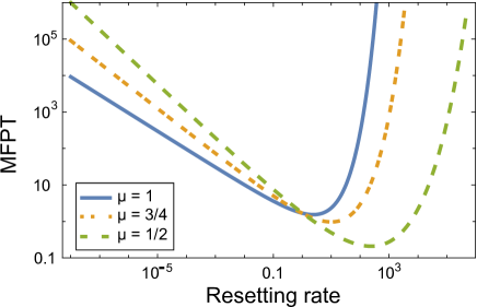
Figure 2: Mean first passage time for general diffusive search process under resetting. MFPT for normal diffusion under stochastic resetting (12) with $\mu=1$ (blue solid line), and MFPT for anomalous diffusion under stochastic resetting (34) with $\mu=3/4$ (red dotted line), and $\mu=1/2$ (green dashed line). The parameters are set as: $D=1$, $x_{0}=1$. In all the cases, we observe an expedited completion due to resetting.

3.5 Heterogeneous diffusion with stochastic resetting

Consider independent random walkers on a one dimensional heterogeneous medium, initially located at position $x_{0}$ and then they search for a target which is located at the origin. The target position defines a bound of the search domain and the process is completed as soon as the target is first detected. The evolution for the probability density function in this case can be written as dos2022efficiency ; sandev2022heterogeneous

$$\frac{\partial P(x,t)}{\partial t}=\frac{\partial^{2}}{\partial x^{2}}\left[D(x)P(x,t)\right]+(A/2-1)\frac{\partial}{\partial x}\left[D^{\prime}(x)P(x,t)\right],$$ (36)

where $D(x)>0$ is a space-dependent diffusion coefficient manifesting for the heterogeneous medium and $0\leq A\leq 2$ is a parameter that takes different values depending on the numerical scheme. For instance, the case of $A=2$ (Itô convention) is commonly used in finance ito1944109 , while $A=1$ (Stratonovich convention) is popular in physics stratonovich1966new . The highly anticipating case $A=0$ (known as isothermal, kinetic, or Hänggi-Klimontovich) also has applications related to Fick’s law hanggi1978stochastic ; klimontovich1990ito ; cherstvy2013anomalous . To mimic the heterogeneous diffusivity, it is often considered $D(x)=D|x|^{\nu}$ ($\nu<2$) which has been used extensively to capture the diffusive motion of a particle on fractal objects and diffusion in turbulent media. For different interpretations of the heterogeneous diffusion processes we refer to ito1944109 ; stratonovich1966new ; hanggi1978stochastic ; klimontovich1990ito ; cherstvy2013anomalous ; leibovich2019infinite ; sandev2022heterogeneous . For this set-up, the survival probability in Laplace space reads dos2022efficiency

$$\widetilde{Q_{0}}(s|x_{0})=\frac{1}{s}-\frac{2}{\Gamma(b)s}\left[\frac{x_{0}^{\frac{2-\nu}{2}}}{2-\nu}\sqrt{\frac{s}{D}}\right]^{b}\times K_{b}\left(\frac{2x_{0}^{\frac{2-\nu}{2}}}{2-\nu}\sqrt{\frac{s}{D}}\right),$$ (37)

where $K_{b}(z)$ is the modified Bessel function and $b=\frac{1-\nu(1-A/2)}{2-\nu}\geq 0$. The MFPT under resetting then can be obtained using Eq. (7)

$$\langle T_{r}\rangle=\frac{1}{r}\left[\frac{\Gamma(b)\left(\frac{x_{0}^{\frac{2-\nu}{2}}}{2-\nu}\sqrt{\frac{r}{D}}\right)^{-b}}{2K_{b}\left(\frac{2x_{0}^{\frac{2-\nu}{2}}}{2-\nu}\sqrt{\frac{r}{D}}\right)}-1\right],$$ (38)

Recalling the definition of the Gamma function, we observe from the above that the MFPT is finite for $b>0$. For the resetting free process, the underlying first passage time density has an asymptotic tail $t^{-b-1}$ which is a generalized version of the simple diffusion case. In such cases, underlying process may have diverging MFPT depending on $\nu$ and $A$. Similar to the cases in the above (eg, diffusion), one can explicitly show that the MFPT becomes finite in the presence of resetting dos2022efficiency ; ray2020space .

4 When resetting works?

There are endless variety of ways in which first passage processes and resetting mechanisms mix and match. Rigorous studies show as is also evident from the examples above that for the processes like diffusion or subdiffusion, resetting always expedites the search while for the search processes in a confined domain or in the presence of a generic potential landscape, resetting can often be detrimental. A lot of efforts has been given in finding the physical conditions which marks this behavioral transition. To see this, one usually looks into a generic first passage process (with well defined first and second moments), add an infinitesimal resetting rate and try to examine its ramifications. Recalling the MFPT under resetting from Eq. (7) and expand it in the following polynomial in the small $r$ limit pal2017first ; pal2019landau

$$\langle T_{r}\rangle=a_{0}+a_{1}r+a_{2}r^{2}+a_{3}r^{3}+\cdots~{},$$ (39)

where $a_{i}$-s are the expansion coefficients. Such kind of expansion respects a set of postulates which we state below. By taking $r$ strictly to be zero, we see that $\langle T_{r}\rangle=a_{0}=\langle T\rangle$, the MFPT of the underlying process in the absence of resetting and is assumed to be positive finite.

Physical meaning of the coefficients.— The coefficients $a_{i}$-s, so far defined formally, can be given physical meaning by analyzing $\langle T_{r}\rangle$ around $r=0$. Recalling $\widetilde{f_{T}}(r|\cdot)=\int_{0}^{\infty}~{}dt~{}e^{-rt}~{}f_{T}(t|\cdot)$ to be the Laplace transformation of the underlying first passage time, expanding the same in the small $r$ limit in Eq. (7) and furthermore comparing with the Taylor’s series expansion of $\langle T_{r}\rangle$ in Eq. 39, we identify $a_{0}=\langle T\rangle,~{}a_{1}=-\frac{\langle T^{2}\rangle}{2}+\langle T\rangle^{2},~{}a_{2}=\frac{1}{6}\langle T^{3}\rangle+\langle T\rangle^{3}-\langle T\rangle\langle T^{2}\rangle,~{}a_{3}=-\frac{\langle T^{4}\rangle}{4!}+\frac{\langle T^{3}\rangle\langle T\rangle}{3}+\frac{\langle T^{2}\rangle^{2}}{4}-\frac{3\langle T^{2}\rangle\langle T\rangle^{2}}{2}+\langle T\rangle^{4}$, and so on where $\langle T^{n}\rangle$ is the $n$-th moment of the underlying first passage time distribution pal2017first ; pal2019landau . The moments (hence the coefficients) are explicit functions of the system parameters, and will characterize the transitions.

A universal criterion.— For resetting to reduce the underlying MFPT, one would naturally expect $\langle T_{r\to 0}\rangle<\langle T_{r=0}\rangle$ with the introduction of resetting. This essentially means from Eq. (39) that in the linear order expansion one must have $a_{1}<0$. Rearranging $a_{1}$ from the above, one finds pal2017first ; pal2019firstbranch

$$CV\equiv\frac{\sigma(T)}{\langle T\rangle}>1$$ (40)

where $CV$ is called the the coefficient of variation. This is a measure of statistical dispersion that stands for the ratio between the standard deviation $\sigma(T)$ and the mean $\langle T\rangle$ of the underlying first passage time $T$. The criterion is completely universal, system independent and essentially tells that for resetting to be beneficial this measure has to be higher than unity. Note that the $CV$-criterion depends only on the first two statistical metrics (which need to be finite) of the underlying process and not the entire distribution. For the stochastic processes, where $CV=\infty$ (broad distribution/heavy tail) or even not well-defined (eg., Lévy first passage time distribution for the 1D simple diffusive search), resetting is guaranteed to help and thus this relation becomes redundant. Clearly, for the underlying first passage processes with narrow distributions (towards a deterministic limit) such that $CV<1$, resetting can only prolong the completion (see Fig. (3)). It is worth noting that the $CV=1$ condition can also be derived from the inspection paradox in probability theory pal2022inspection .

While the $CV$-criterion is the sufficient condition, it is not a necessary one. As seen above, the sign of $a_{1}$ is important to derive this criterion, whereas $a_{2}$ plays the pivotal role for higher order corrections. In such cases, $CV$-criterion need not be respected yet resetting can be found to be useful pal2019landau ; ahmad2023comparing .

Interpretation of the criterion.— The coefficient of variation $(CV)$ usually characterizes how broad or narrow a distribution is around its mean and that certainly depends on the underlying search mechanism, search domain, target configurations and many other intrinsic parameters. Recent single molecule experiments with colloidal particles, biomolecules, enzymes have brought deep insights into the first passage phenomena while looking into various microscopic search mechanism such as surmounting activation barriers, bottlenecks, gated reactions, transport across channels, facilitated diffusion and chemical reactions (see eg satija2020broad ; sturzenegger2018transition ; thorneywork2020direct and metzler2014first for a review). Many such transport, escape or activation processes take place in multidimensional energy landscape with metastable states in the presence of deep kinetic traps and large fluctuating barriers. There, the microscopic searchers tend to spend exceedingly large time and thus the completion time statistics render to heavy tail broad distributions klafter2011first ; bouchaud1990anomalous . Similar arguments also apply to chemical reactions which are inherently stochastic in nature. Thus the outcome of the reactions are also random – this means various kinds of products can be formed from an enzyme due to the intrinsic fluctuations. Enzymatic catalysis process often can take place on-pathways or off/parallel-pathways moffitt2014extracting ; english2006ever . In the former case, the reactions are usually nearest neighbour and the dwell time distribution is narrower. The latter case however can contain multiple pathways with active catalytic states with relative weights. This gives rise to multiple class of dwell time distributions which have long, multi-exponential or heavy tails. Thus the natural reaction time will have broader distributions with $CV>1$. These kind of scenarios also take place when searchers are macroscopic eg. foraging animals, falcons or even drones viswanathan2011physics ; viswanathan1999optimizing . Many such processes take place in unconfined territory in search of a steady supply of nutrients and other essential resources. Indeed, there can be large fluctuations around the average search time due to uncertainty, lack of cognition and experience and these can turn out to be deleterious and may often result in death. As shown above, resetting/quenching to the initial configuration for the microscopic searchers, unbinding of the enzymes from the metastable states or returning to the home for macroscopic searchers can reverse the deleterious effects of large fluctuations in the underlying search time, thus turning a marked drawback into a favorable advantage. Simply put, such reset kind events can curtail the long detrimental trajectories and make the process more regular and remarkably efficient. From a broader perspective, whenever we have $CV>1$ (ie, worse search conditions for the underlying process), physical scenarios naturally suggest that search with resets/returns may be considered as a useful bet-hedging strategy.

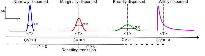
Figure 3: Schematic illustration of the possible roles of resetting on the underlying first passage time processes. For the narrowly dispersed distribution, $CV<1$ and resetting is only detrimental. As $CV$ increases and crosses the boundary $CV=1$, the effect of resetting becomes more significant. Infinite dispersion $CV=\infty$ may arise when the underlying first passage time process is characterized by heavy power law tails (namely $f_{T}(t)\sim t^{-(1+\gamma)}$ with $0<\gamma<2$). Remarkably, in such cases one always observes an overarching gain due to resetting. The interpolation between these behaviors is captured by the optimal resetting rate $r^{*}$ which plays the role of an order parameter. The transition between $r^{*}>0$ and $r^{*}=0$ at the phase-separatrix $CV=1$ is often known as the resetting transition.

Optimal resetting rate as an order parameter and resetting transition.— The equality $CV=1$ serves as a sharp boundary for resetting transition. This is not really a thermodynamic phase transition, but mimics the behavioral transition between the phases namely “resetting-detrimental” and “resetting-beneficial”. Assume $CV<1$ - in this case, $\langle T_{r\to 0}\rangle>\langle T_{r=0}\rangle$ and thus the optimal resetting rate $r^{*}$ that globally minimizes $\langle T_{r}\rangle$ is fixed at zero. In other words, resetting only delays the completion process. On the other hand, for $CV>1$, we have $\langle T_{r\to 0}\rangle<\langle T_{r=0}\rangle$ and thus the optimal resetting rate $r^{*}$ that globally minimizes $\langle T_{r}\rangle$ takes a non-zero value. Simply put, an optimally reset process can always expedite the completion making resetting beneficial. The transition between $r^{*}=0$ to $r^{*}>0$ as we vary $CV$ is known as the “resetting transition” and the optimal resetting rate can be regarded as the order parameter for such transition in resetting systems (see Fig. (3)). Since $CV$ is usually a function of the system parameters, one could imagine that there is a control parameter of interest, say $p$, that can be varied to span from $CV<1$ to $CV>1$. Henceforth, $CV=1$ would render a critical $p_{c}$ in the parameter space where the exact resetting transition will take place. In fact, one can show that near the transition, $r^{*}\sim|p-p_{c}|^{\beta}$, where $\beta=1$ is a critical exponent that is found to be universal across different reset processes pal2019landau ; ahmad2019first . This is somewhat reminiscent of the continuous phase transition in statistical physics. Furthermore, a Landau like mean field approach can be used to probe such universality pal2019landau .

5 Applications of resetting to real world search problems

So far, we discussed the theoretical implications of stochastic resetting on search problems. In this section, we shift our perspective and turn our attention to the applications of stochastic resetting in real-world search problems. In particular, we discuss recent developments on applying resetting to home range search pal2020search ; tal2020experimental , resetting facilitated diffusive transport jain2023fick , turnover of chemical reactions reuveni2014role ; rotbart2015michaelis ; biswas2023rate , and income dynamics jolakoski2023first . This helps us bridge the gap between theoretical research and its tangible applications in real-world scenarios.

5.1 Home range search

One of the intriguing applications of random resetting in search problems is the home range search. In this context, a searcher is not indefinitely adrift in a search space but has a reference point — a “home” — to which it can return under certain conditions. This kind of search strategy finds applications in animal foraging behavior, robot exploration, and many areas where search optimization is crucial.

Imagine a searcher that begins at an origin or “home” in a potentially $d$-dimensional search space $\mathcal{D}$. This searcher attempts to locate a target (or multiple targets). For the unconstrained search, the searcher might find the target in a random time $T$, taken from the distribution $f_{T}(t)$. However, real-world searchers often have limitations or strategies that cause them to return to a starting or known point. In our model, if the searcher does not find the target within a stipulated time $R$ distributed according to $f_{R}(t)=re^{-rt}$, it retreats back to its home. The time it takes to return, denoted as $\tau(\vec{x})$, can vary depending on where the searcher is when the decision to return home is made. Once the searcher reaches home, it might rest or re-strategize, staying there for a time span $W$. Post this, the search initiates anew, making the process cyclic pal2020search .

To make this model tractable, we employ two assumptions. First, targets cannot be located during the phases of return and waiting at home. Second, search cycles are isolated events. This means each new search starts with no memory of past endeavors, thus ensuring independence between cycles. The latter fact allows one to utilize the renewal approach as sketched out in Sec 2 and estimate the MFPT for such home-range-search process which reads pal2020search

$$\langle T_{r}\rangle=\underbrace{\frac{\widetilde{Q_{0}}(r|\vec{x_{0}})}{1-r\widetilde{Q_{0}}(r|\vec{x_{0}})}}_{\text{search}}+\underbrace{\frac{r\int_{\mathcal{D}}d\vec{x}~{}\tau(\vec{x})\widetilde{P}_{0}(\vec{x},r)}{1-r\widetilde{Q_{0}}(r|\vec{x_{0}})}}_{\text{return}}+\underbrace{\frac{r\widetilde{Q_{0}}(r|\vec{x_{0}})}{1-r\widetilde{Q_{0}}(r|\vec{x_{0}})}\langle W\rangle}_{\text{home}},$$ (41)

where $\tau(\vec{x})$ is the home-return time of the searcher starting from the coordinate $\vec{x}$ at the time of resetting. Here, $\widetilde{P}_{0}(\vec{x},r)=\int_{0}^{\infty}dt~{}e^{-rt}P_{0}(\vec{x},t)$ is the LT of $P_{0}(\vec{x},t)$ – PDF of the underlying process such that $Q_{0}(t|\vec{x_{0}})=\int_{\mathcal{D}}~{}d\vec{x}~{}P_{0}(\vec{x},t)$ is the survival probability of the searcher upto time $t$.

Return of a diffusive searcher with a constant velocity

To exemplify Eq. (41), let us consider a one dimensional diffusive search process where the searcher has to find a target placed at $L$. The searcher starts from its home which is fixed at the origin. Let us assume that upon resetting, the searcher returns to its home with a constant velcity $v_{r}$ such that $\tau(x)=|x|/v_{r}$. In this case, elementary calculation yields $\widetilde{P}_{0}(\vec{x},r)=\frac{1}{\sqrt{4Dr}}\left[e^{-\sqrt{r/D}|x|}-e^{-\sqrt{r/D}(2L-x)}\right]$ and thus from Eq. (41) one finds pal2020search

$$\langle T_{r}\rangle=\frac{1}{r}\left(e^{\sqrt{r/D}L}-1\right)+\frac{L}{v_{r}}\left(\frac{2\sinh{(\sqrt{r/D}L)}}{\sqrt{r/D}L}-1\right),$$ (42)

where we have assumed $W=0$ for simplicity. Note that the first term on the RHS is accounted for the search process and thus identical to the MFPT under instantaneous resetting. The second term on the RHS accounts for the delay due to the finite time return to its home. As $v_{r}\to\infty$, one recovers the instantaneous limit since the searcher returns to its home almost instantaneously. See Fig. 4a which shows the modulation of MFPT under different return velocity.

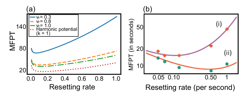
Figure 4: Behaviour of the mean first passage time of a home range diffusive searcher as a function of resetting rate under various modes of return. Panel (a) shows MFPTs when the searcher returns to its home at a constant velocity or is attracted by a harmonic trap centered at its home. Panel (b) shows MFPTs of a silica particle to a target wall under non-instantaneous returns with (i) $\tau_{0}=3.79$s and instantaneous returns with (ii) $\tau_{0}=0$ respectively. Theoretical predictions (Eq. (46), solid lines) are in good agreement with experimental data (symbols). Panel (b) is adapted from tal2020experimental .

Return of a searcher under the action of a harmonic potential

We now consider a return process where a generic one dimensional searcher returns under the influence of a harmonic potential $U(x)=\frac{1}{2}kx^{2}$ such that we can write a Newton’s law for the return process $\ddot{x}=-kx$. This is a deterministic return process and thus the solution of the return path is $x=x_{0}\cos{(\sqrt{k}t)}$, where $x_{0}$ is the starting location. Using this one finds the return time to the origin to be $\tau(x)=\pi/\sqrt{4k}$, which turns out to be independent of $x$. Plugging this in Eq. (41), one finds

$$\langle T_{r}\rangle=\frac{\widetilde{Q_{0}}(r|x_{0})}{1-r\widetilde{Q_{0}}(r|x_{0})}+\frac{\pi}{\sqrt{4k}}\frac{r\widetilde{Q_{0}}(r|x_{0})}{1-r\widetilde{Q_{0}}(r|x_{0})},$$ (43)

which holds for any arbitrary underlying search process. In particular, for diffusive process one has bodrova2020resetting

$$\langle T_{r}\rangle=\left[\frac{1}{r}+\frac{\pi}{\sqrt{4k}}\right]\left(e^{\sqrt{r/D}L}-1\right).$$ (44)

When the stiffness of the potential is very high (ie, $k\to\infty$), one immediately recovers the instantaneous return limit. Otherwise for finite stiffness, it can often facilitate the search compared to the velocity driven return process (see Fig. 4a).

Return in first passage time under fixed time – resetting experiments

We now turn our attention to the case when the searcher returns to its home in fixed time say $\tau_{0}$. This protocol is quite feasible in the single particle experiments since the searcher (say, a silica particle) can be manipulated with great precision by optical traps tal2020experimental . In such case, the MFPT reads

$$\langle T_{r}\rangle=\frac{\widetilde{Q_{0}}(r|x_{0})}{1-r\widetilde{Q_{0}}(r|x_{0})}+\tau_{0}\frac{r\widetilde{Q_{0}}(r|x_{0})}{1-r\widetilde{Q_{0}}(r|x_{0})},$$ (45)

which again holds for any arbitrary underlying search process. In particular, in the first passage time experiment tal2020experimental ], resetting mechanism was conducted stochastically using holographic optical tweezers on a silica particle (which mimics a diffusive dynamics). Following the resetting, the particle was returned to its home (ie, the initial coordinate) using the optical traps in a constant time $\tau_{0}$ tal2020experimental . For a diffusive particle starting from the origin, the above expression for the MFPT to a target set at $L$ simplifies to

$$\langle T_{r}\rangle=\left[\frac{1}{r}+\tau_{0}\right]\left(e^{\sqrt{r/D}L}-1\right),$$ (46)

which was verified against the experimental data to find an excellent fit tal2020experimental . See Fig. 4b which was adapted from tal2020experimental .

Stochastic return of the searcher

Notably, we have assumed that the return to the home is a deterministic process making $\tau(\vec{x})$ a deterministic function once $\vec{x}$ is fixed. One can also consider a situation where the return processes are stochastic. This is natural in many set-ups since there will always be random fluctuations that are uncontrollable and thus return protocols need not be absolutely deterministic. In such cases, $\tau(\vec{x})$ becomes a stochastic function of the return path and thus to emphasize this additional averaging, one needs to replace $\tau(\vec{x})$ by $\overline{\tau(\vec{x})}$ in Eq. (41). Interested readers can take a look at these references gupta2020stochastic ; gupta2021resetting ; biswas2023stochasticity ; mercado2020intermittent for such scenarios.

5.2 Resetting facilitated diffusive transport through channels

Diffusion of particles, molecules, or even living microorganisms in confined geometries such as tubes and channels plays a key role across various scales in natural and technological processes jacobs1935diffusion ; zwanzig1992diffusion . A diffusing particle inside a channel can either escape from both sides of the membrane or it may be allowed to escape through one side while the other side simply reflects it back. Key quantities in these processes are the first passage probabilities and average escape times from the channel (or lifetimes) conditioned to the exit side of the membrane, as well as the overall average lifetime of the particle in the channel berezhkovskii2011time ; berezhkovskii2006identity . These quantities are ubiquitous in theoretical studies on channel-facilitated transport. Enormous theoretical efforts have been devoted over the years to make the transport inside various channels more efficient. The fact that resetting has the ability to speed-up complex search processes naturally compels one to use resetting as a useful strategy for the channel-facilitated first passage transport. Indeed this was shown in jain2023fick recently, and we review the results in brief.

The canonical Fick-Jacobs formalism is a key approach to treat diffusion of particles, ions, molecules, or even living microorganisms in confined geometries such as tubes and channels of varying cross-sections jacobs1935diffusion ; zwanzig1992diffusion ; dagdug2003diffusion . For instance, the effective one-dimensional Fick-Jacobs equation for a diffusing particle, starting at $x_{0}$, inside a three dimensional conical tube of variable radius $R(x)$ and length $L$ can be written as

$$\frac{\partial{P}(x,t)}{\partial t}=\frac{\partial}{\partial x}\left\{D(x)e^{-\beta_{\mathcal{T}}U(x)}\frac{\partial}{\partial x}\left[e^{\beta_{\mathcal{T}}U(x)}P(x,t)\right]\right\},$$ (47)

where the entropy potential is given by -$\beta_{\mathcal{T}}U(x)=\ln(R^{2}(x)/R^{2}(x_{0}))$ for a 3D tube. Here, $\beta_{\mathcal{T}}=1/(k_{B}\mathcal{T})$ is the inverse temperature with $k_{B}$ the Boltzmann constant. Replacing $U(x)$ for the 3D cone, the modified equation reads

$$\frac{\partial{P}(x,t)}{\partial t}= D_{\lambda}\frac{\partial}{\partial x}\left\{R^{2}(x)\frac{\partial}{\partial x}\left[\frac{{P}(x,t)}{R^{2}(x)}\right]\right\},$$ (48)

where $D_{\lambda}$ is given by the Reguera-Rubi formula $D_{\lambda}=\frac{D_{0}}{\sqrt{1+\lambda^{2}}}$ reguera2001kinetic . We further assume that the tube radius $R(x)$ increases in the axial direction with a constant rate $\lambda$ so that $R(x)=a+\lambda x$, where the $x$-coordinate is measured along the tube axis, and $a$ is the tube radius at $x=0$. For a conical tube with two absorbing points at $x=0$ and $x=L$, the unconditional first passage time density (in Laplace space) is given by jain2023fick

$$\widetilde{f_{T}}(s|x_{0})=\frac{(\lambda L+a)\sinh(\sqrt{s/D_{\lambda}}x_{0})+a\sinh(\sqrt{s/D_{\lambda}}(L-x_{0}))}{(\lambda x_{0}+a)\sinh(\sqrt{s/D_{\lambda}}L)}.$$ (49)

The first passage density can then be substituted in Eq. (7) to obtain the MFPT of the searcher in the presence of resetting jain2023fick

$$\langle T_{r}(x_{0})\rangle=\frac{(\lambda x_{0}+a)\sinh(\alpha_{\lambda}L)-a\sinh(\alpha_{\lambda}(L-x_{0}))-(\lambda L+a)\sinh(\alpha_{\lambda}x_{0})}{r[a\sinh(\alpha_{\lambda}(L-x_{0}))+(\lambda L+a)\sinh(\alpha_{\lambda}x_{0})]},$$ (50)

where $\alpha_{\lambda}=\sqrt{r/D_{\lambda}}$. It can further be shown using the $CV$-criterion ( 40) that resetting is going to be beneficial (i.e., an optimal resetting rate $r^{*}>0$ would exist) when the following condition is satisfied jain2023fick

$$(\lambda v+\tilde{a})\left[\lambda(1+v)(7-3v^{2})+15\tilde{a}(1+v-v^{2})\right]\geq 10v(1-v)\left[\lambda(1+v)+3\tilde{a}\right]^{2},$$ (51)

where $\tilde{a}=a/L$ and $v=x_{0}/L$. Thus, the criterion is fulfilled as long as the particle starts sufficiently close to one of the absorbing boundaries ($v\sim 0$ or $v\sim 1$) but not when it starts out in the center. For starting positions near the center of the tube, increasing the reset rate increases the MFPT since any trajectory on both sides is going to take particle closer to the boundary and reset hinders it. But for starting positions closer to the boundaries, resetting decreases the lifetime because there are now many more possible trajectories that are taking the particle away from the boundary and resetting systematically eliminates them jain2023fick . A carefully navigated resetting strategy thus can facilitate diffusive transport through narrow channels. Likewise, resetting can also be useful for active transport and search in a confined arena sar2023resetting .

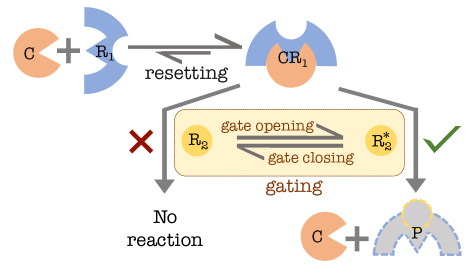
Figure 5: Scheme for a gated chemical reaction between two reactants $R_{1}$ and $R_{2}$, catalysed by $C$. Initially, the catalyst binds reversibly with $R_{1}$ to generate $CR_{1}$, a metastable intermediate: $C+R_{1}\stackrel{{\scriptstyle}}{{\rightleftharpoons}}CR_{1}$. In the next step, $CR_{1}$ reacts selectively with $R^{\star}_{2}$ (the reactive or open-gate state of $R_{2}$) to generate the product $P$ and liberate the catalyst: $CR_{1}+R_{2}^{\star}\to C+P$. This step can be modeled by gated drift-diffusion, while the unbinding of $C$ from $R_{1}$ is essentially manifested as resetting. Adapted from biswas2023rate .

5.3 Turnover of the gated chemical reactions

For a reaction, two molecules first need to meet by overcoming the activation barrier between them. Since the motion of the molecules are stochastic, these reactions are inherently stochastic in nature and estimation of the reaction-time is often cast as a first passage problem english2006ever ; iyer2016first ; metzler2014first ; moffitt2014extracting . Chemical reactions usually comprise of three basic steps: binding (when one reactant $C$ binds another one $R_{1}$ to form a metastable complex $CR_{1}$), unbinding or resetting (when the complex $CR_{1}$ is disassociated to the parent reactants) and catalysis (when a product $P$ is successfully formed). Often, the reactant molecules switch between a reactive and a non-reactive state; and thus the collisions between the reactants must happen in their reactive states for the completion of a successful product formation (see Fig. 5). This is known as ‘gating’ in biochemistry that typically refers to the transition between the open and closed states of an ion channel; and the ions are allowed to flow through the channel only when it is open bressloff2014stochastic ; szabo1982stochastically .

Such gated reactions can be illustrated by considering a diffusive transport process confined to the positive semi-infinite space in the presence of a target that randomly switches between an open and a closed state with constant rates. Consider that the target switches from the non-reactive to the reactive state at a rate $\gamma>0$, and the reverse transition takes place with a constant rate $\beta>0$. This is a general scenario mimicked by, e.g., a chemical reaction (see Fig. 5), where the collisions between reactants [$CR_{1}$ and $R_{2}$] lead to the formation of product only when at least one of the reactants is in an activated state [when $R_{2}$ exists as $R_{2}^{\star}$] and not otherwise. Since resetting is an integral part of any consecutive chemical reaction that has a reversible first-step [when $C$ binds to, or unbinds from, $R_{1}$], the reaction scheme shown in Fig. 1 can be modeled as gated diffusion process in a potential landscape with resetting. The mean turnover time of this reaction can then be obtained by casting into the formulation shown above biswas2023rate ; mercado2021search

$$\langle T_{r}^{G}\rangle=\frac{e^{\sqrt{\frac{r}{D}}x_{0}}-1}{r}+\frac{\beta e^{\sqrt{\frac{r}{D}}x_{0}}}{\gamma\sqrt{r[r+\gamma+\beta]}}\mbox{}\left[1+\frac{re^{-\sqrt{\frac{r+\gamma+\beta}{D}}x_{0}}}{(\gamma+\beta)}\right].$$ (52)

It can be shown explicitly that resetting or unbinding is always going to expedite the turnover process compared to the underlying gated diffusive process biswas2023rate ; mercado2021search .

5.4 Resetting in income dynamics

Income mobility describes the dynamic aspects of income within a society. Formally, it quantifies the time it takes for an individual to transition from one income status to another, shedding light on the pace and accessibility of upward mobility in different societies JanttiJenkins2015 ; stojkoski2022measures ; stojkoski2022ergodicity ; la2023unraveling .

Recently, it was shown that a first passage under resetting approach to income dynamics can effectively capture micro-level variations and experiences of individuals, a caveat that is often missing in standard income mobility analyses. The idea is that a baseline model for income dynamics called geometric Brownian motion with stochastic resetting and allows us to develop a “model” based view for quantifying the time needed for an individual currently with income $x_{0}$ to reach target income $y$ gabaix2016dynamics ; nirei2004income ; aoki2017zipf ; stojkoski2022income ; vinod2022nonergodicity ; vinod2022time .

In this application, the particle position $x(t)$ can be thought of as the income of a worker in period $t$ (Fig. 6(a)). This observable grows multiplicatively with a rate $\mu$ and volatility $\sigma$ cherstvy2017time ; stojkoski2020generalised ; stojkoski2019cooperation ; kemp2022statistical ; kemp2023learning until a random event that occurs with a rate $r$ resets its dynamics evans2011diffusion . The reset event can be interpreted as a worker that left the job market (for example by retiring, being laid off, or after an injury) and is substituted by another younger worker with a starting income $x_{R}$ (here, $x_{R}$ need not be equal to $x_{0}$) nirei2004income . Hence, the MFPT in srGBM disaggregates the income dynamics to the level of individual workers, offering a more nuanced lens through which we can understand the intricacies of income mobility.

To derive the MFPT in srGBM we use the Fokker-Planck equation for the distribution of the random income variable $x(t)$ that follows the geometric Brownian motion with $r=0$. This equation reads

$$\frac{\partial}{\partial t}P(x,t)=\mathcal{L}(x)P(x,t)~{},$$ (53)

where $\mathcal{L}(z)=\mu z\frac{\partial}{\partial z}+\frac{\sigma^{2}}{2}z^{2}\frac{\partial^{2}}{\partial z^{2}}$ is the generator for the GBM process (following Itô convention) stojkoski2020generalised ; stojkoski2021geometric . For Stratonovich and Hänggi-Klimontovich convention of the GBM we refer to sandev2020hitting ; sandev2023special . Using this equation and the general formalism for first passage, it can be shown that the Laplace form of the solution for the mean first passage time of a GBM trajectory to reach a finite income target $y$, starting at $x_{0}$, is

$$\widetilde{f_{T}}(s|x_{0}) =\left(\frac{x_{0}}{y}\right)^{q_{1}(s)},\quad x_{0}\leq y,$$ (54)

$$q_{1}(s) =\frac{\sqrt{(\sigma^{2}-2\mu)^{2}+8s\sigma^{2}}+(\sigma^{2}-2\mu)}{2\sigma^{2}}>0.$$ (55)

Substituting the above in Eq. (7), one obtains the MFPT of a srGBM trajectory that stochastically resets to $x_{R}$.

Applying the srGBM framework to study the income dynamics yields enlightening observations. For instance, as the economy experiences a larger growth of income or larger volatility, the MFPT declines, as illustrated in Fig. 6(b-c). This observation aligns with real-world insights: it is generally easier for workers to traverse the income distribution when the economy booms and there is increased randomnessaristei2015drivers .

The stochastic resetting rate $r$ in the srGBM framework provides another layer of depth to our understanding (depicted with red dots in Fig. 6(b-c)). This rate, especially when optimized at $r^{*}$, can be perceived as a lever that policymakers might tweak to influence the rhythm of income dynamics within an economy. For instance, by calibrating policies around workforce participation - such as the frequency of retirements - authorities could potentially regulate the time it takes for a worker to navigate the income spectrum cremer2004social ; staubli2013does ; sheather2021great . Two salient features of the optimal resetting rate in srGBM emerge which mirror real-world economic observations. First, when volatility is held constant, a surge in growth ($\mu$) reduces the rate at which MFPT reaches its minimum. This, for example, could be a result of joint factors leading to economic growth such as efficient qualification programs, or quality foreign investments. Second, for a fixed growth rate, when the randomness in the system is increased, we also observe an increased optimal resetting rate. This, for example, can be a result of increased intrinsic differences between societal groups when it comes to getting new jobs (e.g., gender or racial differentials).

These theoretical insights have led to an empirical methodology for using the srGBM MFPT in real economies jolakoski2023first ; stojkoski2023income . By integrating the srGBM framework with data, a more textured landscape of income dynamics and economic mobility emerges, paving the way for richer insights and more informed policy decisions. The simplicity of the srGBM MFPT approach paves the way for potential applications in other countries, opening doors to global economic insights.

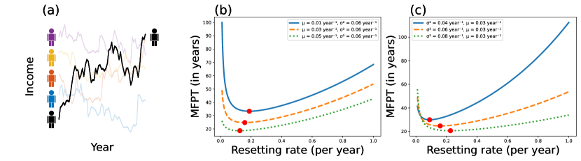
Figure 6: Resetting in income dynamics. Panel (a): A schematic figure for the income movement of an individual over the years. Panel (b): MFPT (in years) as a function of the resetting rate for various growth rates $\mu$. Panel (c): MFPT (in years) as a function of the resetting rate for various volatilities $\sigma^{2}$. For panels (b-c): We set $x_{0}=x_{R}=1$ and $y=2$. Adapted from jolakoski2023first .

6 Discussion

In this chapter we have shown that stopping a complex search process intermittently only to reset or restart from scratch can often lead to an accelerated completion – a counter-intuitive effect that is orthogonal to our general perception. The subject of random resetting has been a topical interest and has seen a wide panorama of applications starting from physics, chemistry, biology, ecology, computer science to economics. Developing a comprehensive framework for the first passage statistics under resetting, we have applied the formalism to many diffusive and non-diffusive theoretical first passage models. In doing so, we discuss in detail the conditions which play a pivotal role in determining whether resetting can be indeed be used as a mitigating strategy. Finally, we showcase a few interdisciplinary applications of resetting motivated by the real world search processes.

It will be quite interesting to study various non-Markovian complex search processes eg geometry-controlled kinetics benichou2010geometry , random walks in fractal geometry condamin2007first under generic resetting mechanism. Yet another interesting direction that remains quite less explored is the thermodynamical cost of first passage resetting (see pal2021thermodynamic ; PhysRevE.108.044117 ; gupta2020work ). For instance, what will be the energy expenditure for an optimally reset process in comparison to a simply reset process? Will there be a universal thermodynamic trade-off relation at the optimality? Naturally, these questions are fundamental to design resetting strategies in living systems. Needless to say, with the current advent of the experimental studies using laser traps goerlich2023experimental ; tal2020experimental ; besga2020optimal , tunable robots paramanick2023programming ; altshuler2023environmental or the applications of resetting in quantum search processes yin2023restart ; kulkarni2023first , queuing theory bonomo2022mitigating & material science aquino2023fluid , the field marks the inception of a new era where we expect to see more realistic and trans-disciplinary applications of resetting in complex systems.

- (1) M.R. Evans, S.N. Majumdar, G. Schehr, J. Phys. A: Math. Theor. 53(19), 193001 (2020)
- (2) M.R. Evans, S.N. Majumdar, Phys. Rev. Lett. 106(16), 160601 (2011)
- (3) A. Pal, Phys. Rev. E 91(1), 012113 (2015)
- (4) M.R. Evans, S.N. Majumdar, K. Mallick, J. Phys. A: Math. Theor. 46(18), 185001 (2013)
- (5) S. Eule, J.J. Metzger, New Journal of Physics 18(3), 033006 (2016)
- (6) A. Nagar, S. Gupta, Physical Review E 93(6), 060102 (2016)
- (7) V. Méndez, D. Campos, Phys. Rev. E 93(2), 022106 (2016)
- (8) A. Kumar, A. Pal, Physical Review Letters 130(15), 157101 (2023)
- (9) L. Kusmierz, S.N. Majumdar, S. Sabhapandit, G. Schehr, Phys. Rev. Lett. 113(22), 220602 (2014)
- (10) O.L. Bonomo, A. Pal, Physical Review E 103, 052129 (2021)
- (11) S. Belan, Phys. Rev. Lett. 120(8), 080601 (2018)
- (12) M.R. Evans, S.N. Majumdar, J. Phys. A: Math. Theor. 44(43), 435001 (2011)
- (13) A. Pal, S. Reuveni, Phys. Rev. Lett. 118(3), 030603 (2017)
- (14) S. Reuveni, Phys. Rev. Lett. 116(17), 170601 (2016)
- (15) A. Chechkin, I. Sokolov, Phys. Rev. Lett. 121(5), 050601 (2018)
- (16) A. Pal, Ł. Kuśmierz, S. Reuveni, Physical Review Research 2(4), 043174 (2020)
- (17) O. Tal-Friedman, A. Pal, A. Sekhon, S. Reuveni, Y. Roichman, The journal of physical chemistry letters 11(17), 7350 (2020)
- (18) B. Besga, A. Bovon, A. Petrosyan, S.N. Majumdar, S. Ciliberto, Phys. Rev. Research 2(3), 032029 (2020)
- (19) V. Stojkoski, P. Jolakoski, A. Pal, T. Sandev, L. Kocarev, R. Metzler, Philos. Trans. R. Soc. A 380(2224), 20210157 (2022)
- (20) X. Gabaix, J.M. Lasry, P.L. Lions, B. Moll, Econometrica 84(6), 2071 (2016)
- (21) D. Vinod, A.G. Cherstvy, W. Wang, R. Metzler, I.M. Sokolov, Phys. Rev. E 105(1), L012106 (2022)
- (22) P. Jolakoski, A. Pal, T. Sandev, L. Kocarev, R. Metzler, V. Stojkoski, Chaos, Solitons & Fractals 175, 113921 (2023)
- (23) D. Boyer, C. Solis-Salas, Physical review letters 112(24), 240601 (2014)
- (24) É. Roldán, A. Lisica, D. Sánchez-Taltavull, S.W. Grill, Physical Review E 93(6), 062411 (2016)
- (25) A.M. Ramoso, J.A. Magalang, D. Sánchez-Taltavull, J.P. Esguerra, É. Roldán, Europhysics Letters 132(5), 50003 (2020)
- (26) S. Budnar, K.B. Husain, G.A. Gomez, M. Naghibosadat, A. Varma, S. Verma, N.A. Hamilton, R.G. Morris, et al., Developmental cell 49(6), 894 (2019)
- (27) S. Reuveni, M. Urbakh, J. Klafter, Proc. Natl. Acad. Sci. 111(12), 4391 (2014)
- (28) T. Rotbart, S. Reuveni, M. Urbakh, Phys. Rev. E 92(6), 060101 (2015)
- (29) A. Biswas, A. Pal, D. Mondal, S. Ray, The Journal of Chemical Physics 159(5) (2023)
- (30) A. Morán, M. Lihoreau, A. Pérez-Escudero, J. Gautrais, PLOS Computational Biology 19(3), e1010558 (2023)
- (31) O. Bénichou, C. Loverdo, M. Moreau, R. Voituriez, Reviews of Modern Physics 83(1), 81 (2011)
- (32) A. Ray, A. Pal, D. Ghosh, S.K. Dana, C. Hens, Chaos: An Interdisciplinary Journal of Nonlinear Science 31(1) (2021)
- (33) O.L. Bonomo, A. Pal, S. Reuveni, PNAS Nexus 1(3), pgac070 (2022)
- (34) M. Luby, A. Sinclair, D. Zuckerman, Information Processing Letters 47(4), 173 (1993)
- (35) O. Blumer, S. Reuveni, B. Hirshberg, The journal of physical chemistry letters 13(48), 11230 (2022)
- (36) A. Pal, A. Kundu, M.R. Evans, Journal of Physics A: Mathematical and Theoretical 49(22), 225001 (2016)
- (37) S. Redner, A guide to first-passage processes (Cambridge University Press, 2001)
- (38) A.J. Bray, S.N. Majumdar, G. Schehr, Advances in Physics 62(3), 225 (2013)
- (39) V. Stojkoski, T. Sandev, L. Kocarev, A. Pal, Journal of Physics A: Mathematical and Theoretical 55(10), 104003 (2022)
- (40) M.R. Evans, S.N. Majumdar, Journal of Physics A: Mathematical and Theoretical 47(28), 285001 (2014)
- (41) A. Pal, R. Chatterjee, S. Reuveni, A. Kundu, Journal of Physics A: Mathematical and Theoretical 52(26), 264002 (2019)
- (42) R. Singh, R. Metzler, T. Sandev, J. Phys. A: Math. Theor. 53(50), 505003 (2020)
- (43) S. Ray, D. Mondal, S. Reuveni, Journal of Physics A: Mathematical and Theoretical 52(25), 255002 (2019)
- (44) D. Gupta, C.A. Plata, A. Kundu, A. Pal, J. Phys. A: Math. Theor. 54(2), 025003 (2020)
- (45) S. Ahmad, I. Nayak, A. Bansal, A. Nandi, D. Das, Phys. Rev. E 99(2), 022130 (2019)
- (46) V.F. Zaitsev, A.D. Polyanin, Handbook of exact solutions for ordinary differential equations (CRC press, 2002)
- (47) S. Ray, S. Reuveni, The Journal of chemical physics 152(23) (2020)
- (48) K. Capała, B. Dybiec, arXiv preprint arXiv:2305.14832 (2023)
- (49) A. Pal, V. Prasad, Phys. Rev. E 99(3), 032123 (2019)
- (50) A. Pal, V. Prasad, Phys. Rev. Research 1(3), 032001 (2019)
- (51) S. Ahmad, K. Rijal, D. Das, Physical Review E 105(4), 044134 (2022)
- (52) H. Chen, F. Huang, Physical Review E 105(3), 034109 (2022)
- (53) S. Ahmad, D. Das, Physical Review E 102(3), 032145 (2020)
- (54) S. Ahmad, D. Das, Journal of Physics A: Mathematical and Theoretical 56(10), 104001 (2023)
- (55) A. Chatterjee, C. Christou, A. Schadschneider, Physical Review E 97(6), 062106 (2018)
- (56) K. Capała, B. Dybiec, Journal of Statistical Mechanics: Theory and Experiment 2021(8), 083216 (2021)
- (57) R. Metzler, J. Klafter, Phys. Rep. 339(1), 1 (2000)
- (58) J. Klafter, I.M. Sokolov, First steps in random walks: from tools to applications (OUP Oxford, 2011)
- (59) V. Méndez, A. Masó-Puigdellosas, T. Sandev, D. Campos, Physical Review E 103(2), 022103 (2021)
- (60) V. Méndez, A. Masó-Puigdellosas, D. Campos, Physical Review E 105(5), 054118 (2022)
- (61) I.M. Sokolov, J. Klafter, Chaos: An Interdisciplinary Journal of Nonlinear Science 15(2) (2005)
- (62) A. Stanislavsky, A. Weron, Physical Review E 104(1), 014125 (2021)
- (63) A. Masó-Puigdellosas, D. Campos, V. Méndez, Phys. Rev. E 99(1), 012141 (2019)
- (64) J. Masoliver, M. Montero, Phys. Rev. E 100(4), 042103 (2019)
- (65) Ł. Kuśmierz, E. Gudowska-Nowak, Phys. Rev. E 99(5), 052116 (2019)
- (66) V. Shkilev, Physical Review E 96(1), 012126 (2017)
- (67) M. Dos Santos, L. Menon Jr, C. Anteneodo, Physical Review E 106(4), 044113 (2022)
- (68) T. Sandev, V. Domazetoski, L. Kocarev, R. Metzler, A. Chechkin, Journal of Physics A: Mathematical and Theoretical 55(7), 074003 (2022)
- (69) K. Itô, Proceedings of the Imperial Academy 20(8), 519 (1944)
- (70) R. Stratonovich, SIAM Journal on Control 4(2), 362 (1966)
- (71) P. Hänggi, Helv. Phys. Acta 51, 183 (1978)
- (72) Y.L. Klimontovich, Physica A: Statistical Mechanics and its Applications 163(2), 515 (1990)
- (73) A.G. Cherstvy, A.V. Chechkin, R. Metzler, New Journal of Physics 15(8), 083039 (2013)
- (74) N. Leibovich, E. Barkai, Physical Review E 99(4), 042138 (2019)
- (75) S. Ray, J. Chem. Phys. 153(23), 234904 (2020)
- (76) A. Pal, I. Eliazar, S. Reuveni, Phys. Rev. Lett. 122(2), 020602 (2019)
- (77) A. Pal, S. Kostinski, S. Reuveni, Journal of Physics A: Mathematical and Theoretical 55(2), 021001 (2022)
- (78) R. Satija, A.M. Berezhkovskii, D.E. Makarov, Proceedings of the National Academy of Sciences 117(44), 27116 (2020)
- (79) F. Sturzenegger, F. Zosel, E.D. Holmstrom, K.J. Buholzer, D.E. Makarov, D. Nettels, B. Schuler, Nature communications 9(1), 4708 (2018)
- (80) A.L. Thorneywork, J. Gladrow, Y. Qing, M. Rico-Pasto, F. Ritort, H. Bayley, A.B. Kolomeisky, U.F. Keyser, Science advances 6(18), eaaz4642 (2020)
- (81) R. Metzler, S. Redner, G. Oshanin, First-passage phenomena and their applications, vol. 35 (World Scientific, 2014)
- (82) J.P. Bouchaud, A. Georges, Physics reports 195(4-5), 127 (1990)
- (83) J.R. Moffitt, C. Bustamante, The FEBS journal 281(2), 498 (2014)
- (84) B.P. English, W. Min, A.M. Van Oijen, K.T. Lee, G. Luo, H. Sun, B.J. Cherayil, S. Kou, X.S. Xie, Nature chemical biology 2(2), 87 (2006)
- (85) G.M. Viswanathan, M.G. Da Luz, E.P. Raposo, H.E. Stanley, The physics of foraging: an introduction to random searches and biological encounters (Cambridge University Press, 2011)
- (86) G.M. Viswanathan, S.V. Buldyrev, S. Havlin, M. Da Luz, E. Raposo, H.E. Stanley, nature 401(6756), 911 (1999)
- (87) S. Jain, D. Boyer, A. Pal, L. Dagdug, The Journal of Chemical Physics 158(5) (2023)
- (88) A.S. Bodrova, I.M. Sokolov, Physical Review E 101(5), 052130 (2020)
- (89) D. Gupta, A. Pal, A. Kundu, Journal of Statistical Mechanics: Theory and Experiment 2021(4), 043202 (2021)
- (90) A. Biswas, A. Kundu, A. Pal, arXiv preprint arXiv:2307.16294 (2023)
- (91) G. Mercado-Vásquez, D. Boyer, S.N. Majumdar, G. Schehr, Journal of Statistical Mechanics: Theory and Experiment 2020(11), 113203 (2020)
- (92) M.H. Jacobs, M. Jacobs, Diffusion processes (Springer, 1935)
- (93) R. Zwanzig, The Journal of Physical Chemistry 96(10), 3926 (1992)
- (94) A. Berezhkovskii, A. Szabo, The Journal of chemical physics 135(7) (2011)
- (95) A.M. Berezhkovskii, G. Hummer, S.M. Bezrukov, Physical review letters 97(2), 020601 (2006)
- (96) L. Dagdug, A. Berezhkovskii, S.M. Bezrukov, G.H. Weiss, The Journal of chemical physics 118(5), 2367 (2003)
- (97) D. Reguera, J. Rubi, Physical Review E 64(6), 061106 (2001)
- (98) G.K. Sar, A. Ray, D. Ghosh, C. Hens, A. Pal, Soft Matter 19, 4502 (2023)
- (99) S. Iyer-Biswas, A. Zilman, Advances in chemical physics 160, 261 (2016)
- (100) P.C. Bressloff, Stochastic processes in cell biology, vol. 41 (Springer, 2014)
- (101) A. Szabo, D. Shoup, S.H. Northrup, J.A. McCammon, The Journal of Chemical Physics 77(9), 4484 (1982)
- (102) G. Mercado-Vásquez, D. Boyer, Journal of Physics A: Mathematical and Theoretical 54(44), 444002 (2021)
- (103) M. Jäntti, S.P. Jenkins, in Handbook of Income Distribution, vol. 2 (Elsevier, 2015), pp. 807–935
- (104) V. Stojkoski, arXiv preprint arXiv:2205.02800 (2022)
- (105) V. Stojkoski, M. Karbevski, Phys. Rev. E 105(2), 024107 (2022)
- (106) C.A. La Porta, S. Zapperi, Journal of Physics: Complexity (2023)
- (107) M. Nirei, W. Souma, in The Complex Dynamics of Economic Interaction (Springer, 2004), pp. 161–168
- (108) S. Aoki, M. Nirei, Am. Econ. J. Macroecon. 9(3), 36 (2017)
- (109) D. Vinod, A.G. Cherstvy, R. Metzler, I.M. Sokolov, Physical Review E 106(3), 034137 (2022)
- (110) A.G. Cherstvy, D. Vinod, E. Aghion, A.V. Chechkin, R. Metzler, New J. Phys. 19(6), 063045 (2017)
- (111) V. Stojkoski, T. Sandev, L. Basnarkov, L. Kocarev, R. Metzler, Entropy 22(12), 1432 (2020)
- (112) V. Stojkoski, Z. Utkovski, L. Basnarkov, L. Kocarev, Phys. Rev. E 99(6), 062312 (2019)
- (113) J.T. Kemp, L.M. Bettencourt, Physica A: Statistical Mechanics and its Applications 607, 128180 (2022)
- (114) J.T. Kemp, L.M. Bettencourt, PNAS nexus 2(4), pgad093 (2023)
- (115) V. Stojkoski, T. Sandev, L. Kocarev, A. Pal, Phys. Rev. E 104(1), 014121 (2021)
- (116) T. Sandev, A. Iomin, L. Kocarev, Phys. Rev. E 102(4), 042109 (2020)
- (117) T. Sandev, A. Iomin, Special Functions of Fractional Calculus: Applications to Diffusion and Random Search Processes (World Scientific, 2022)
- (118) D. Aristei, C. Perugini, Economic Systems 39(2), 197 (2015)
- (119) H. Cremer, J.M. Lozachmeur, P. Pestieau, J. Public Econ. 88(11), 2259 (2004)
- (120) S. Staubli, J. Zweimüller, J. Public Econ. 108, 17 (2013)
- (121) J. Sheather, D. Slattery, BMJ 375(2533) (2021)
- (122) V. Stojkoski, S. Mitikj, M. Trpkova-Nestorovska, D. Tevdovski, Income mobility and mixing in north macedonia. Tech. rep. (2023)
- (123) C. Chevalier, B. Meyer, Nature chemistry 2(6), 472 (2010)
- (124) S. Condamin, O. Bénichou, V. Tejedor, R. Voituriez, Nature 450(7166), 77 (2007)
- (125) A. Pal, S. Reuveni, S. Rahav, Physical Review Research 3(1), 013273 (2021)
- (126) P.S. Pal, A. Pal, H. Park, J.S. Lee, Phys. Rev. E 108, 044117 (2023). DOI 10.1103/PhysRevE.108.044117. URL https://link.aps.org/doi/10.1103/PhysRevE.108.044117
- (127) D. Gupta, C.A. Plata, A. Pal, Phys. Rev. Lett. 124(11), 110608 (2020)
- (128) R. Goerlich, M. Li, L.B. Pires, P.A. Hervieux, G. Manfredi, C. Genet, arXiv preprint arXiv:2306.09503 (2023)
- (129) S. Paramanick, A. Pal, H. Soni, N. Kumar, arXiv preprint arXiv:2306.06609 (2023)
- (130) A. Altshuler, O.L. Bonomo, N. Gorohovsky, S. Marchini, E. Rosen, O. Tal-Friedman, S. Reuveni, Y. Roichman, arXiv preprint arXiv:2306.12126 (2023)
- (131) R. Yin, E. Barkai, Physical Review Letters 130(5), 050802 (2023)
- (132) M. Kulkarni, S.N. Majumdar, arXiv preprint arXiv:2305.15123 (2023)
- (133) T. Aquino, T. Le Borgne, J. Heyman, Physical Review Letters 130(26), 264001 (2023)