Rational function approximation with normalized positive denominators

Abstract

Rational function approximations provide a simple but flexible alternative to polynomial approximation, allowing one to capture complex non-linearities without oscillatory artifacts. However, there have been few attempts to use rational functions on noisy data due to the likelihood of creating spurious singularities. To avoid the creation of singularities, we use Bernstein polynomials and appropriate conditions on their coefficients to force the denominator to be strictly positive. While this reduces the range of rational polynomials that can be expressed, it keeps all the benefits of rational functions while maintaining the robustness of polynomial approximation in noisy data scenarios.

Our numerical experiments on noisy data show that existing rational approximation methods continually produce spurious poles inside the approximation domain. This contrasts our method, which cannot create poles in the approximation domain and provides better fits than a polynomial approximation and even penalized splines on functions with multiple variables. Moreover, guaranteeing pole-free in an interval is critical for estimating non-constant coefficients when numerically solving differential equations using spectral methods. This provides a compact representation of the original differential equation, allowing numeric solvers to achieve high accuracy quickly, as seen in our experiments.

Keywords Rational approximation  $\cdot$ Suprious poles  $\cdot$ Spectral methods  $\cdot$ Data analysis  $\cdot$ Derivative penalty

1 Introduction

Function approximation involves approximating a target function $f:\mathbb{R}\to\mathbb{R}$ with a ‘simpler’ function $g:\mathbb{R}\to\mathbb{R}$. This can be done for reasons including machine learning [1, 2, 3, 4] and numerical computations of transcendental functions [5, 6]. A simple method is to approximate $f(x)$ as a degree $n$ polynomial

$$f(x)\approx g(x)\in\mathcal{P}(n),\quad\text{where}\quad\mathcal{P}(n)=\{\text{Polynomials of degree }n\}.$$ (1)

However, polynomial approximations suffer from Runge’s phenomenon [7, 8, 9], where the approximated function contains oscillatory artifacts that the original function does not have. Piecewise polynomial methods, known as polynomial splines, are typically used to reduce such effects, with penalized splines (piecewise cubic polynomials with a penalty term) being a popular method.

Instead, $f$ can be approximated as a rational polynomial

$$f(x)\approx r(x)=\frac{p(x)}{q(x)},\quad\text{where}\quad p(x)\in\mathcal{P}(n)\ \text{and}\ q(x)\in\mathcal{P}(m),$$ (2)

and we denote $\mathcal{R}(n,m)=\{p(x)/q(x)\ |\ p(x)\in\mathcal{P}(n)\ \text{and}\ q(x)\in\mathcal{P}(m)\}$ as the space of $(n,m)$ rational polynomials.

As mentioned, rational function approximation is advantageous in numerous applications because of the enhanced opportunity for compression compared to standard polynomial methods. However, a particular application originally motivated our current work. As an example, we envision solving a non-constant coefficient differential equation

$$\sum_{k=0}^{K}c_{k}(x)\,D^{k}u(x)\ =\ f(x).$$ (3)

where we assume $f(x)\in\mathcal{P}(n)$ for some $n$. Chebyshev spectral methods are a common approach to equations of this form [10, 11, 12]. In that case, the solution is expanded in terms of polynomial basis functions, and the derivatives map sparsely to an alternative basis set. The catch is that we must expand the non-constant coefficients, $c_{k}(x)$, in a polynomial basis and promote the result to matrix operations. Such an approach works especially well in one-dimension [13, 14, 15, 16, 17, 18] where the typical degree of a coefficient, $c_{k}(x)$ is much less than the requirements of the solution, e.g., $\sim 10$ versus $\sim 1000$ respectively. The downside is that the final overall matrix representation becomes evermore dense with each additional polynomial degree of the highest resolve of the coefficients; the matrix bandwidth scales with the degree. The cubic scaling of operator bandwidth throttles the overall algorithm. The problem is even more stark in multiple dimensions [19, 20, 21, 22, 23, 24].

This is where a rational approximation could come in handy. Suppose we could represent the coefficients as

$$c_{k}(x)\ =\ \frac{p_{k,N}(x)}{q_{M}(x)},\quad\text{where}\quad p_{k,N}(x)\in\mathcal{P}(N),\quad q_{M}(x)\in\mathcal{P}(M).$$ (4)

The point is that if all the coefficients have a common denominator, $q_{M}(x)$, independent of $k$, then we can possibly reduce the maximum degree of all the numerators, $\deg(p_{k,N})\leq N$ for all $k$. We can then clear the denominator and solve more sparsely

$$\sum_{k=0}^{K}p_{k,N}(x)\,D^{k}u(x)\ =\ q_{M}(x)\,f(x).$$ (5)

We discuss applications like this and more in our examples section.

Of course, rational functions are good for many things other things, such as accurate estimations to nonsmooth and non-Lipschitz functions [25] and better approximations than ordinary polynomials [26]. However, an important difficulty can arise if the $q_{M}(x)$ has roots or near roots in the relevant part of the domain. As such, they have seldom been applied to noisy data, perhaps because they are fragile and have little control over the pole locations [26, 27, 28].

To that end, we propose the Bernstein Denominator Algorithm, where we force $q(x)>0$ in the approximation interval by using Bernstein polynomials with normalized and positive coefficients. This provides a robust method to produce rational approximations without poles in the approximation domain. This method works well on noisy data, consistently producing approximations without poles while other rational approximations do. Moreover, it provides a more flexible method than penalized splines on functions of multiple variables while reducing Runge’s phenomenon.

2 Previous Works

A simple way of representing rational polynomials in $\mathcal{R}(n,m)$ is in the form

$$r(x)=\frac{p(x)}{q(x)}=\frac{a_{0}+a_{1}x+\cdots+a_{n}x^{n}}{b_{0}+b_{1}x+\cdots+b_{m}x^{m}}.$$ (6)

But this form is invariant under rescalings of the numerator and denominator, leading to non-unique solutions. A normalizing factor, $b_{0}=1$, is thus introduced resulting in the form

$$r(x)=\frac{p(x)}{q(x)}=\frac{a_{0}+a_{1}x+\cdots+a_{n}x^{n}}{1+b_{1}x+\cdots+b_{m}x^{m}}.$$ (7)

However, there is a significant amount of work [29, 30, 31, 32, 26, 33] on Rational Barycentric forms

$$r(x)=\frac{n(x)}{d(x)}=\sum_{k=1}^{n}\frac{w_{k}f_{k}}{x-x_{k}}\bigg{/}\sum_{k=1}^{n}\frac{w_{k}}{x-x_{k}},$$ (8)

with $f_{k}\in\mathbb{C}$ and $w_{k}\in\mathbb{C}$ and nonzero. As shown in [29], these forms range over the set of $\mathcal{R}(n-1,n-1)$ that have no poles at the points $x_{k}$. Moreover, they have the property that $r(x_{k})=f_{k}$ for all $k$.

Using one of these two forms, methods in rational function approximation can be split into either an interpolation problem or a least square fit problem.

2.1 Interpolation

For a partition $0\leq x_{1}<\cdots<x_{J}\leq 1$ of the unit interval, interpolation of a target function $f(x)$ involves finding a rational function such that

$$f(x_{j})=r(x_{j}),\quad\text{for}\quad 1\leq j\leq J.$$ (9)

Polynomial forms solve this problem by assuming $q(x_{j})\neq 0$ for all $j$. This allows one to multiply $q(x)$ on each side of (9), thus linearizing the problem into

$$a_{0}+a_{1}x_{i}+\cdots a_{n}x_{i}^{n}=f(x_{i})(1+b_{1}x_{i}+\cdots+b_{m}x_{i}^{m}),\quad\text{for}\quad 1\leq j\leq J.$$ (10)

Requiring interpolation at $J=m+n+1$ points yields $m+n+1$ equations for $m+n+1$ unknown coefficients. This can then be solved using standard methods, like LU decomposition.

Barycentric forms provides a simple way of interpolation due to their unique property that $r(x_{k})=f_{k}$, where $r(x)$ is defined in (8). Interpolation can therefore occur by setting $f_{k}=f(x_{k})$ for $1\leq k\leq J$. However, the weights $w_{k}$ still need to be found.

The AAA algorithm, by Nakatsukasa, Sète, and Trefethen [29], finds weights that minimize the residuals

$$\min_{w\in S^{J-1}}\sum_{i}\varepsilon_{i}^{2},\quad\text{where}\quad S^{J-1}=\{w\in\mathbb{R}^{J}\ |\ \|w\|=1\},$$ (11)

$$\text{and}\ \varepsilon_{i}=n(z_{i})-f(z_{i})d(z_{i})=\sum_{k=1}^{J}\frac{w_{k}f_{k}}{z_{i}-x_{k}}-f(z_{i})\sum_{k=1}^{J}\frac{w_{k}}{z_{i}-x_{k}},$$ (12)

on a set of distinct support points $\{z_{i}\}_{i}$ with $z_{i}\neq x_{k}$ for all $i,k$. When $|\{z_{i}\}_{i}|\geq J$, a unique minimizer can be found using singular value decomposition (SVD).

Poleless Barycentric Forms were first considered by Berrut [28], in which Berrut takes $w_{k}=(-1)^{k+1}$ for $1\leq k\leq J$. As Berrut shows, this results in a rational polynomial without poles in $\mathbb{R}$. This was then further generalized by Floater and Hormann [26] into the form

$$r(x)=\frac{\sum_{i=1}^{J-d}\lambda_{i}(x)p_{i}(x)}{\sum_{i=1}^{J-d}\lambda_{i}(x)},\quad\text{for some}\quad 0\leq d\leq J-1,$$ (13)

and for $1\leq i\leq J-d$, $p_{i}$ is the unique polynomial of degree $d$ that interpolates $f$ at the points $x_{i},\ldots,x_{i+d}$, and

$$\lambda_{i}(x)=\frac{(-1)^{i+1}}{(x-x_{i})\cdots(x-x_{i+d})}.$$ (14)

2.2 Least Square Fits

Rather than requiring exact fits at the points $x_{i}$, least squares fit aims to minimize the squared residuals

$$\min_{\begin{subarray}{c}a_{0},\ldots,a_{n}\\ b_{1},\ldots,b_{m}\end{subarray}}\sum_{i}\epsilon_{i}^{2},\quad\text{where}\quad\epsilon_{i}=f(x_{i})-\frac{p(x_{i})}{q(x_{i})}.$$ (15)

Like interpolation, it is often assumed that $q(x_{i})\neq 0$ allowing one to minimize the weighted residuals

$$\min_{\begin{subarray}{c}a_{0},\ldots,a_{n}\\ b_{1},\ldots,b_{m}\end{subarray}}\sum_{i}\varepsilon_{i}^{2},\quad\text{where}\quad\varepsilon_{i}=q(x_{i})\epsilon_{i}=p(x_{i})-f(x_{i})q(x_{i}).$$ (16)

Least square fits have the added advantage that equality at the points $x_{i}$ is unnecessary, only that it is ‘close’ to the true value. This allows us to generalize the problem to finding a rational polynomial that best fits an input-output pair $\{(x_{i},y_{i})\}_{1\leq i\leq J}$, where $x_{i}\in[0,1]$, $y_{i}=f(x_{i})+z_{i}$ and $z_{i}$ is a random variable with $\mathbb{E}[z_{i}]=0$. Giving the optimization problem

$$\min_{\begin{subarray}{c}a_{0},\ldots,a_{n}\\ b_{1},\ldots b_{m}\end{subarray}}\sum_{i}\varepsilon_{i}^{2},\quad\text{where}\quad\varepsilon_{i}=p(x_{i})-y_{i}q(x_{i}).$$ (17)

Assuming $J\geq n+m+1$, a unique solution can be found using SVD.

The SK Algorithm was introduced by Sanathanan and Koerner [34] to reduce the deficiencies present in this formulation. They note that the weighted residuals $\varepsilon_{i}$ would result in bad fits for lower frequency values and larger errors when $q(x)$ has poles in the complex plane. Instead, they consider an iterative procedure in which, at iteration $t$, one minimizes the reweighted residuals

$$\min_{\begin{subarray}{c}a_{0},\ldots,a_{n}\\ b_{1},\ldots,b_{m}\end{subarray}}\sum_{i}\mathcal{E}_{t,i}^{2},\quad\text{where}\quad\mathcal{E}_{t,i}=\frac{\varepsilon_{t,i}}{q_{t-1}(x_{i})}=\frac{p_{t}(x_{i})-y_{i}q_{t}(x_{i})}{q_{t-1}(x_{i})},$$ (18)

which provides a better reflection of the original rational approximation problem (15) [35]. Taking $q_{0}(x)=1$ for the first iteration, each iteration can similarly be solved using SVD.

The Quasiconvex Algorithm, introduced by Peiris et al. [36] in 2021, takes a step at preventing singularities in the approximation by forcing positivity in the denominator at each evaluation point $x_{i}$. They consider the constrained optimization problem

$$\min_{\begin{subarray}{c}a_{0},\ldots,a_{n}\\ b_{0},b_{1},\ldots,b_{m}\end{subarray}}\max_{i}\bigg{|}y_{i}-\frac{p(x_{i})}{q(x_{i})}\bigg{|},\quad\text{such that}\quad b_{0}\geq 0,\text{ and }\,\delta\leq q(x_{i})\leq\zeta\text{ for all }i,$$ (19)

for some small $\delta>0$ and finite $\zeta\gg 1$. This is then framed as a new constrained optimization problem

$$\min_{\begin{subarray}{c}a_{0},\ldots,a_{n}\\ b_{0},b_{1},\ldots,b_{m}\end{subarray}}z,\quad\text{such that}$$ (20)

$$y_{i}-\frac{p(x_{i})}{q(x_{i})}\leq z,\quad\frac{p(x_{i})}{q(x_{i})}-y_{i}\leq z,\quad\delta\leq q(x_{i})\leq\zeta\quad\text{ for all }i,\text{ and }\quad b_{0}\geq 0.$$ (21)

As Periris et al. remark, this problem is non-convex when $z$ is a variable. Instead, if there exists polynomials $p(x)$ and $q(x)$ that satisfy (21) for a fixed $z=\hat{z}\geq 0$, then the optimal solution is bounded by $\hat{z}$. If such a $\hat{z}$ exists, then the following linear programming problem

$$\min_{\begin{subarray}{c}a_{0},\ldots,a_{n}\\ b_{0},b_{1},\ldots,b_{m}\end{subarray}}\theta,\quad\text{such that}$$ (22)

$$(y_{i}-\hat{z})q(x_{i})-p(x_{i})\leq\theta,\quad p(x_{i})-(y_{i}+\hat{z})q(x_{i})\leq\theta,\quad\delta\leq q(x_{i})\leq\zeta,\quad\forall i,\quad\text{and}\quad b_{0}\geq 0,$$ (23)

has a solution with $\theta\leq 0$. Conversely, if such a $\hat{z}$ doesn’t exist, then this will have a solution with $\theta>0$. By iteratively proposing various values for $\hat{z}$ and solving the linear programming problem (22)-(23), they obtain an approximate solution to (20)-(21) within a certain tolerance.

2.3 Padé Approximation

While the previously mentioned algorithms focus on approximating $f(x)$ through its value at certain points $x_{i}$, the Padé approximation approximates $f(x)$ through its derivatives. In particular, the Padé approximator produces a rational function

$$r(x)=\frac{a_{0}+a_{1}x+\cdots a_{n}x^{n}}{1+b_{1}x+\cdots+b_{m}x^{m}},$$ (24)

such that the Taylor series of $r(x)$ matches with the Taylor series of $f(x)$ around $x=0$ to as high degree as possible. In particular, these coefficients can be chosen to agree, at least, to the $(m+n)$-th derivatives of $f(x)$ [37].

One major benefit of the Padé approximation is that it may converge when the corresponding Taylor series doesn’t. Even when the Taylor series does converge, the corresponding Padé approximation may converge faster. The Padé approximation thus becomes a powerful tool in asymptotic methods, which finds solutions as a power series. As such, while our work doesn’t focus on Padé approximations, we present it here as it is of historical importance, having found use when studying quantum mechanics, numerical analysis, and quantum field theory [38, 39].

3 Rational Bernstein Denominator Algorithm

In this paper, we are concerned with finding rational function approximations

$$f(x)\ \approx\ {\mathtt{R}}_{N,M}(x)\ =\ \frac{{\mathtt{N}}_{N}(x)}{{\mathtt{D}}_{M}(x)}\quad\text{for}\quad x\in[0,1],$$ (25)

with the major caveat that we want to ensure strict positivity in the denominator,

$${\mathtt{D}}_{M}(x)\ >\ 0\quad\text{for}\quad x\in[0,1].$$ (26)

This is a key differentiation between our work and those that came before, in that we are interested in representing smooth functions, $f(x)$, that are guaranteed to be pole-free in $[0,1]$ using rational functions. We are not interested in representing a larger class of functions.

For the denominator, we introduce the family of "Bernstein basis" polynomials for $x\in[0,1]$,

$$\mathcal{B}^{(n)}_{k}(x)=\binom{n}{k}x^{k}(1-x)^{n-k},\quad\text{where}\quad 0\leq k\leq n.$$ (27)

Bernstein [40] used this basis in a probabilistic proof of the Weierstrass approximation theorem. That is, for a continuous function on the unit interval, $q(x)$,

$$q(x)\ \approx\ \sum_{k=0}^{n}q(k/n)\,\mathcal{B}_{k}^{(n)}(x)\ =\ \mathbb{E}(q(x)),$$ (28)

where the expectation of the right-hand side is right with respect to the Binomial probability distribution. The Weak Law of Large Numbers implies the result. While (28) is known to have slow convergence [41], this is not a problem for our particular application. The Bernstein polynomials are used to ensure positivity in the denominator.

The denominator is thus represented as a weighted Bernstein series

$${\mathtt{D}}_{M}(x)\ =\ \sum_{m=0}^{M}w_{m}\,\mathcal{B}_{m}^{(M)}(x).$$ (29)

The positivity of ${\mathtt{D}}_{M}$ can be guaranteed by forcing

$$w_{m}\ \geq\ 0.$$ (30)

However, as with other rational function methods, this has the issue of non-uniqueness under rescaling ${\mathtt{N}}_{N}\to c\,{\mathtt{N}}_{N}$, ${\mathtt{D}}_{M}\to c\,{\mathtt{D}}_{M}$ for $c\neq 0$ leaves $R_{N,M}$ unchanged. To this end, the denominator is normalized by also requiring

$$\sum_{m=0}^{M}w_{m}\ =\ 1.$$ (31)

Both conditions together imply the weights lie in a probability simplex

$$\Delta^{M+1}\ =\ \left\{w\in\mathbb{R}^{M+1}\ \bigg{|}\ 0\leq w_{m}\leq 1\ \text{and}\ \sum_{m=0}^{M}w_{m}=1\right\}.$$ (32)

The numerator is represented as

$${\mathtt{N}}_{N}(x)\ =\ \sum_{n=0}^{N}a_{n}\,p_{n}(x),\quad\text{where}\quad a_{n}\in\mathbb{R},$$ (33)

given a suitable family of basis functions (usually orthogonal polynomials). No additional constraints on the spectral coefficients $a_{n}$ are needed as the denominator is normalized.

Thus, we consider rational functions of the form

$$f(x)\ \approx\ {\mathtt{R}}_{N,M}(x)\ =\ \sum_{n=0}^{N}\,a_{n}\,p_{n}(x)\ \bigg{/}\ \sum_{m=0}^{M}\,w_{m}\,\mathcal{B}_{m}(x)$$ (34)

with $w\in\Delta^{M+1}$ and $a\in\mathbb{R}^{N+1}$.

3.1 Lagrange’s Polynomial Root Bound

Another way to guarantee rational approximations without roots in $[0,1]$ is to use bounds on the roots of polynomials. In particular, for a $n$-degree polynomial,

$$p(x)\ =\ a_{0}\,+\,a_{1}x\,+\,\cdots\,+\,a_{n}x^{n},$$ (35)

Lagrange’s Bound states that the magnitudes of it’s $n$-roots, $\{x_{i}\}_{1\leq i\leq n}$, can be bounded by

$$\frac{1}{\max\bigg{\{}1,\ \sum_{i=1}^{n}\,\left|{a_{i}}/{a_{0}}\right|\bigg{\}}}\ \leq\ |x_{i}|\quad\text{for}\quad 1\leq i\leq n.$$ (36)

Since we care about polynomials in the normalized denominator, i.e. $a_{0}=1$, to be free of poles in $[0,1]$, one can consider polynomials of the form

$$\widetilde{\mathcal{P}}(n)\ =\ \bigg{\{}1\,+\,a_{1}x\,+\,\cdots\,+\,a_{n}x^{n},\quad\text{with}\quad\sum_{i=1}^{n}\,|a_{i}|\ \leq\ 1\bigg{\}},$$ (37)

to guarantee no roots inside $[0,1]$. However, the Bernstein formulation is a superset of this problem.

Remark 1.

Without loss of generality, we can consider the closure of $\widetilde{\mathcal{P}}(n)$. That is, polynomials of the form

$$\overline{\mathcal{P}}(n)\ =\ \bigg{\{}1\,+\,a_{1}x\,+\,\cdots\,+\,a_{n}x^{n},\quad\text{with}\quad\sum_{i=1}^{n}|a_{i}|\ =\ 1\bigg{\}},$$ (38)

as any polynomial in $\widetilde{\mathcal{P}}(n)$ can be written as

$$p(x)\ :=\ 1\,+\,a_{1}x\,+\,\cdots\,+\,x_{n}x^{n}\ =\ (1-c)\ +\ c\left(1+\frac{a_{1}}{c}x+\cdots+\frac{a_{n}}{c}x^{n}\right),$$ (39)

where $c=\sum_{i}|a_{i}|\leq 1$. It follows that $\sum_{i}|a_{i}/c|=1$, and

$$q(x)\ :=\ 1+\frac{a_{1}}{c}x+\cdots+\frac{a_{n}}{c}x^{n}\ \in\ \overline{\mathcal{P}}(n).$$ (40)

By properties of the Bernstein polynomials,

$$\sum_{j=0}^{n}\,\mathcal{B}^{(n)}_{j}(x)\ =\ 1\quad\text{for all}\quad x\in[0,1].$$ (41)

We can therefore write $p(x)$ as

$$p(x)\ =\ (1-c)\,\sum_{j=0}^{n}\,\mathcal{B}^{(n)}_{j}(x)\ +c\,q(x).$$ (42)

Thus, if all polynomials in $\overline{\mathcal{P}}(n)$ can be written in terms of Bernstein basis polynomials with positive coefficients, so can polynomials in $\widetilde{\mathcal{P}}(n)$.

Theorem 1.

Any polynomial in $\overline{\mathcal{P}}(n)$ has an equivalent Bernstein basis representation with coefficients that are all positive, i.e., there exist Bernstein coefficients $b_{i}\geq 0$ such that

$$p(x)\ :=\ 1+a_{1}x+\cdots+a_{n}x^{n}\ =\ \sum_{i=0}^{n}\,b_{i}\,\mathcal{B}^{(n)}_{i}(x),\quad\text{with}\quad\sum_{i=1}^{n}\,|a_{i}|\ =\ 1.$$ (43)

Proof.

Since $p\in\overline{\mathcal{P}}(n)$, then $\sum_{i}|a_{i}|=1$, and hence

$$p(x)\ =\ 1\ +\ \sum_{a_{i}\geq 0}\,|a_{i}|\,x^{i}\ -\ \sum_{a_{i}<0}\,|a_{i}|\,x^{i},$$ (44)

$$=\ \sum_{a_{i}\geq 0}\,|a_{i}|\,(1+x^{i})\ +\ \sum_{a_{i}<0}\,|a_{i}|\,(1-x^{i}).$$ (45)

Thus, to account for the sign, these polynomials can be written as a convex combination of

$$M_{i,\pm}(x)\ =\ 1\pm x^{i},\quad\text{for}\quad 1\leq i\leq n,$$ (46)

with positive weight given to one of $M_{i,\pm}$ with the correct sign and zero to the other. That is, there exists positive weights, $w_{i,s}\geq 0$, such that

$$1+a_{1}x+\cdots+a_{n}x^{n}\ =\ \sum_{s\in\{+,-\}}\,\sum_{i=1}^{n}\,w_{i,s}\,M_{i,s}(x)\quad\text{and}\quad\sum_{s\in\{+,-\}}\,\sum_{i=1}^{n}\,w_{i,s}\ =\ 1.$$ (47)

From the Binomial and Vandermonde’s identity, the monomial coefficients, $a_{j}$, expressed in Bernstein coefficients via,

$$b_{j}\ =\ \sum_{k=0}^{j}\frac{\binom{j}{k}}{\binom{n}{k}}a_{k}.$$ (48)

Then

$$M_{i,\pm}(x)\ =\ 1\pm x^{i}\ =\ \sum_{j}\,b_{j}\,\mathcal{B}^{(n)}_{j}(x)\quad\text{where}\quad b_{j}\ =\ 1\pm\frac{\binom{j}{i}}{\binom{n}{i}}\mathbbm{1}_{i\leq j},$$ (49)

and $\mathbbm{1}_{i\leq j}=1$ if $i\leq j$ and $0$ otherwise. It is clear that $b_{j}\geq 0$ for $M_{i,+}$. For $M_{i,-}$, since $j\leq n$, it follows from the geometric interpretation of combinations that

$$\binom{j}{i}\leq\binom{n}{i}.$$ (50)

Thus $b_{j}\geq 0$ for $M_{i,\pm}$. Hence, each basis function, $M_{i,\pm}$, represents a positively weighted sum of Bernstein polynomials.

Since every polynomial in $\overline{\mathcal{P}}(n)$ can be written as a convex combination of $M_{i,\pm}$, it follows that it also can be written as a convex combination of Bernstein polynomials with positive coefficients. Thus, every polynomial in $\overline{\mathcal{P}}(n)$ can be written as a sum of Bernstein polynomials with positive coefficients. ∎

Remark 2.

There exist positive-normalized Bernstein basis polynomials that yield a Lagrange bound less than one. As a simple counter-example, consider the normalized Bernstein polynomial

$$p(x):=\frac{1}{2}\mathcal{B}_{0}^{(n)}(x)\ +\ \frac{1}{2}\mathcal{B}_{n}^{(n)}(x),$$ (51)

for $n\geq 2$. This has no roots in $[0,1]$.

By expanding the Bernstein polynomials using the Binomial theorem and comparing coefficients, the Bernstein coefficients, $b_{i}$, can be converted to monomial coefficients, $a_{i}$, via

$$a_{j}\ =\ \sum_{k=0}^{j}\,(-1)^{j-k}\,\binom{n}{j}\,\binom{j}{k}\,b_{k}.$$ (52)

Explicitly, the monomial coefficients are therefore given by

$$a_{0}\ =\ \frac{1}{2},\quad a_{j}\ =\ (-1)^{j}\,\frac{1}{2}\,\binom{n}{j}\quad\text{for}\quad 1\leq j\leq n-1,\quad\text{and}\quad a_{n}\ =\ \frac{(-1)^{n}\ +1}{2}.$$ (53)

Now,

$$\sum_{j=1}^{n}\,\bigg{|}\frac{a_{j}}{a_{0}}\bigg{|}\ \geq\ \bigg{|}\frac{a_{1}}{a_{0}}\bigg{|}\ =\ \binom{n}{1}\ =\ n.$$ (54)

Therefore, Lagrange’s lower bound can be bounded by

$$\frac{1}{\max\bigg{\{}1,\sum_{j=1}^{n}|a_{j}/a_{0}|\bigg{\}}}\ \leq\ \frac{1}{n}\ <\ 1.$$ (55)

As such, a normalized-positive Bernstein basis polynomial exists in which Lagrange’s lower bound yields a bound on the magnitudes of the roots that is less than one.

Remark 3.

We can instead use Cauchy’s bound, which says that the magnitude of the roots has a lower bound given by

$$\frac{1}{1+\max\bigg{\{}{a_{1}}/{a_{0}},\ldots,a_{n}/a_{0}\bigg{\}}}.$$ (56)

However, this always results in roots with a lower bound inside $[0,1]$.

Remark 4.

While Lagrange and Cauchy’s bound yield bounds on roots within a radius of the origin, the Bernstein polynomials offer an alternative way to bound roots on the positive real line. In particular, for a given monomial

$$p(x)\ =\ a_{0}\,+\,a_{1}x\,+\,\cdots\,+a_{n}x^{n},$$ (57)

if the Bernstein coefficients

$$b_{j}\ =\ \sum_{k=0}^{j}\ \frac{\binom{j}{k}}{\binom{n}{k}}\ a_{k},$$ (58)

are all positive for $0\leq j\leq n$, then there are no roots in $(0,1)$. If $b_{0}=0$, there is a root at $x=0$ and none otherwise. Similarly, if $b_{n}=0$, there is a root at $x=1$ and none otherwise.

Remark 5.

To try and guarantee rational fits without poles, one can use a method presented by the previous works, like the AAA or SK algorithm, and check for poles afterward. However, root-finding algorithms can be unstable, giving inaccurate results [42, 43].

3.2 Residuals

To find the coefficients $w\in\Delta^{M+1}$ and $a\in\mathbb{R}^{N+1}$ we take the least squares approach and minimize a loss function between the target function and the rational function

$$\mathcal{L}(f,{\mathtt{R}}_{N,M}\,|\,a,w).$$ (59)

As done in previous works, the most classic formulation of this loss function is the linearized residuals

$$\mathcal{L}_{\ell}(f,{\mathtt{R}}_{N,M}\,|\,a,w)\ =\ \bigg{\|}f(x)\sum_{m=0}^{M}\,w_{m}\,\mathcal{B}_{m}(x)\ -\ \sum_{n=0}^{N}\,a_{n}\,p_{n}(x)\bigg{\|}^{2}$$ (60)

$$=\ \int_{0}^{1}\left(f(x)\sum_{m=0}^{M}\,w_{m}\,\mathcal{B}_{m}(x)\ -\ \sum_{n=0}^{N}\,a_{n}\,p_{n}(x)\right)^{2}\,d\mu,$$ (61)

for some measure $\mu$. For numerical computations of this integral, we use a discrete measure, yielding

$$\mathcal{L}_{\ell}(f,{\mathtt{R}}_{N,M}\,|\,a,w)\ =\ \sum_{i=0}^{I}\,\mu_{i}\,\left(f(x_{i})\sum_{m=0}^{M}\,w_{m}\,\mathcal{B}_{m}(x_{i})\ -\ \sum_{n=0}^{N}\,a_{n}\,p_{n}(x_{i})\right)^{2},$$ (62)

for a partition of the unit interval $\{x_{i}\}_{0\leq i\leq I}$, and $\{\mu_{i}\}_{0\leq i\leq I}$ are weights that can come from a numerical quadrature formula. This formulation has the advantage of being linear in both $w$ and $a$, becoming a standard quadratic programming problem. It can thus be solved using standard solvers.

However, linearized residuals don’t often reflect the nonlinear residuals well [35]. Instead, following Sanathanan and Koerner, one can consider an iterative algorithm where, on the $t$-th iteration, we minimize the reweighted loss

$$\mathcal{L}_{\ell,t}(f,{\mathtt{R}}_{N,M}\,|\,a,w)\ =\ \int_{0}^{1}\left(f(x)\sum_{m=0}^{M}\,w_{m}\,\mathcal{B}_{m}(x)\ -\ \sum_{n=0}^{N}\,a_{n}\,p_{n}(x)\right)^{2}\,\frac{d\mu}{(\sum_{m=0}^{M}w_{m}^{t-1}\mathcal{B}_{m}(x))^{2}}.$$ (63)

The strict positivity in the denominator, however, offers leniency in being well-defined. Thus, we can consider the nonlinear residuals

$$\mathcal{L}_{r}(f,{\mathtt{R}}_{N,M}\,|\,a,w)\ =\ \bigg{\|}f(x)\ -\ \sum_{n=0}^{N}\,a_{n}\,p_{n}(x)\bigg{/}\sum_{m=0}^{M}\,w_{m}\,\mathcal{B}_{m}(x)\bigg{\|}$$ (64)

$$=\ \int_{0}^{1}\left(f(x)\ -\ \sum_{n=0}^{N}\,a_{n}\,p_{n}(x)\bigg{/}\sum_{m=0}^{M}\,w_{m}\,\mathcal{B}_{m}(x)\right)^{2}\,d\mu.$$ (65)

3.2.1 On the Residuals

The intuition behind the SK algorithm becomes evident when we rewrite the nonlinear residuals as

$$\mathcal{L}_{r}(f,{\mathtt{R}}_{N,M}\,|\,a,w)\ =\ \int_{0}^{1}\left(f(x)\sum_{m=0}^{M}\,w_{m}\,\mathcal{B}_{m}(x)\ -\ \sum_{n=0}^{N}\,a_{n}\,p_{n}(x)\right)^{2}\,\frac{d\mu}{(\sum_{m=0}^{M}w_{m}\mathcal{B}_{m}(x))^{2}}.$$ (66)

Thus, the nonlinear residuals are the linearized residuals with a dynamic measure, and minimizing the linearized residuals does not amount to minimizing the nonlinear residuals. The SK algorithm comes closer to the nonlinear residuals by updating the measure at each iteration. This is reminiscent of greedy algorithms, which take the optimal step at each stage. However, this may not result in optimal solutions [44].

3.3 Sobolev-Jacobi Smoothing

While Runge’s phenomenon is reduced in rational approximations, it can still be particularly pronounced in noisy data scenarios. To that end, a systematic way to enforce smoothing on the rational function must be introduced. Borrowing the idea from penalized splines [45], the smoothness of the approximated function can be enforced by penalizing the L2-norm on its derivatives. However, since the denominator in our formulation is so restrictive, we only apply this penalty to the numerator, i.e., a polynomial. As such, we introduce a new smoothing penalty for polynomial approximation.

Consider the Sobolev inner product

$$\langle f,g\rangle_{\mathcal{H}}\ =\ \sum_{k\geq 0}\,\lambda_{k}\,\int_{\Omega}\,f^{(k)}(x)\,g^{(k)}(x)\,d\rho_{k},$$ (67)

for functions $f$ and $g$, constants $\lambda_{k}\geq 0$, $\Omega\subseteq\mathbb{R}$ and $\rho_{k}$ are measures over $\Omega$. The generalized smoothness penalty on an $N$-degree polynomial, ${\mathtt{P}}_{N}(x)$, is the norm induced by the inner product,

$$\langle{\mathtt{P}}_{N},{\mathtt{P}}_{N}\rangle_{\mathcal{H}}\ =\ \sum_{k\geq 0}\lambda_{k}\ \int_{\Omega}\left(\sum_{n=0}^{N}\,a_{n}\,p_{n}^{(k)}(x)\right)^{2}\ d\rho_{k},$$ (68)

for some set of basis functions $\{p_{n}\}$.

Sobolev orthogonal polynomials are orthogonal with respect to this inner product, with notable examples being classical orthogonal polynomials, as their derivatives are also orthogonal. In particular for the finite domain $\Omega=[0,1]$ the shifted Jacobi polynomials, $\widetilde{P}_{n}^{(a,b)}(x)$, defined on $[0,1]$ with $a,b>-1$, satisfies the relation

$$\int^{1}_{0}\,\frac{d^{k}}{dx^{k}}\widetilde{{P}}_{n}^{(a,b)}(x)\,\frac{d^{k}}{dx^{k}}\,\widetilde{{P}}^{(a,b)}_{m}(x)\,(1-x)^{a+k}\,x^{b+k}\,dx\ =\ c_{n}^{(k)}\,\delta_{n,m}\quad\text{where}$$ (69)

$$c_{n}^{(k)}\ =\ \begin{cases}\cfrac{\Gamma(n+a+1)\,\Gamma(n+b+1)\,\Gamma(n+k+a+b+1)}{(2n+a+b+1)\,(n-k)!\,\Gamma(n+a+b+1)^{2}}&\quad\text{if}\quad 0\leq k\leq n\\ 0&\quad\text{otherwise}.\end{cases}$$ (70)

Then, asymptotically, for $0\leq k\leq n$

$$c_{n}^{(k)}\ \sim\ \frac{\Gamma(n+k+a+b+1)}{(2n+a+b+1)\,(n-k)!}.$$ (71)

Taking $p_{n}$ in equation (68) as the Jacobi polynomial, $\widetilde{P}_{n}^{(a,b)}$, with the corresponding measure, $\rho_{k}$, orthogonality thus yields

$$\langle{\mathtt{P}}_{n},{\mathtt{P}}_{n}\rangle_{\mathcal{H}}\ =\ \sum_{n=0}^{N}\,a_{n}^{2}\,\sum_{k=0}^{n}\lambda_{k}\,c_{n}^{(k)}$$ (72)

$$\sim\ \sum_{n=0}^{N}\,a_{n}^{2}\,\lambda_{n}\,\frac{\Gamma(2n+a+b+1)}{(2n+a+b+1)}$$ (73)

$$\sim\ \sum_{n=0}^{N}\,a_{n}^{2}\,\lambda_{n}\,(2n)^{2n},$$ (74)

by Stirling’s approximation.

Thus, in local coordinates (parameterized by Jacobi polynomials, and thus also Gegenbauer, Legendre, and Chebyshev polynomials [46]), the norm induced by the Sobelev inner product becomes a weighted $\ell^{2}$ norm on the spectral coefficients, with the coefficients being exponentially damped. That is, an exponential penalty on its spectral coefficients can create a smooth polynomial approximation. To reduce the likelihood of overflow errors in the computations, we take $\lambda_{n}=2^{-2n}\,n^{-n}$. This yields what we call the Sobolov-Jacobi smoothing penalty for polynomial approximation

$$\mathcal{R}({\mathtt{P}}_{N})\ =\ \sum_{n=0}^{N}\,a_{n}^{2}\,\,n^{n}.$$ (75)

3.4 Multivariate

So far, we have only considered functions of a single variable. However, the ability to model functions of multiple variables has wide applications in various areas of social sciences (see [47] and the references within). To this end, we generalize our rational function to suit this case. That is, we want rational functions of the form

$${\mathtt{R}}(x_{1},\ldots,x_{s})\ =\ \frac{{\mathtt{N}}(x_{1},\ldots,x_{s})}{{\mathtt{D}}(x_{1},\ldots,x_{s})},$$ (76)

with the restriction that

$${\mathtt{D}}(x_{1},\ldots,x_{s})\ >\ 0\quad\text{for all}\quad(x_{1},\ldots,x_{s})\ \in\ [0,1]^{s}.$$ (77)

To enforce positivity in the denominator, we use a tensor product of Bernstein polynomials

$${\mathtt{D}}(x_{1},\ldots,x_{2}\,|\,w)\ =\ \sum_{m_{1}=0}^{M_{1}}\cdots\sum_{m_{s}=0}^{M_{s}}w_{m_{1},\ldots,m_{s}}\,\mathcal{B}_{m_{1}}(x_{1})\cdots\,\mathcal{B}_{m_{s}}(x_{s}).$$ (78)

Then, positivity and normalization are enforced via the constraints

$$w_{m_{1},\ldots,m_{s}}\ \geq\ 0\quad\text{and}\quad\sum_{m_{1},\ldots,m_{s}}w_{m_{1},\ldots,m_{s}}\ =\ 1.$$ (79)

The numerator is represented as a tensor product of a polynomial basis, $\{p_{n}\}$

$${\mathtt{N}}(x_{1},\ldots,x_{s}\,|\,a)\ =\ \sum_{n_{1}=0}^{N_{1}}\cdots\sum_{n_{s}=0}^{N_{s}}\,a_{n_{1},\ldots,n_{s}}\,p_{n_{1}}(x_{1})\cdots\,p_{n_{s}}(x_{s}).$$ (80)

The linearized, reweighted, and non-linear residuals to minimize are easily generalized.

Taking the shifted Jacobi polynomials as the basis for the numerator, we generalize the smoothing penalty as

$$\mathcal{R}({\mathtt{N}})\ =\ \sum_{n_{1}=0}^{N_{1}}\,\cdots\,\sum_{n_{s}=0}^{N_{s}}\ a_{n_{1},\ldots,n_{s}}^{2}\,n_{1}^{n_{1}}\ \cdots\ n_{s}^{n_{s}}.$$ (81)

3.5 Optimization

To find the coefficients for the rational Bernstein Denominator approximation, ${\mathtt{R}}(x_{1},\ldots,x_{s})$, we consider the constrained optimization problem

$$\min_{\begin{subarray}{c}a\in\mathbb{R}^{{N}^{\prime}}\\ w\in\Delta^{{M}^{\prime}}\end{subarray}}\ \mathcal{L}(f,{\mathtt{R}}\,|\,a,w)\ +\ \lambda\,\mathcal{R}({\mathtt{N}}),$$ (82)

where ${N}^{\prime}=s+N_{1}+\cdots+N_{s}$, ${M}^{\prime}=s+M_{1}+\cdots+M_{s}$, some smoothing strength $\lambda\geq 0$, and $\mathcal{L}$ can be the linearized residuals, $\mathcal{L}_{\ell}$, the reweighted residuals, $\mathcal{L}_{\ell,t}$, or the nonlinear residuals, $\mathcal{L}_{r}$.

Taking $\mathcal{L}$ as the linearized or reweighted residuals has the advantage of being a standard quadratic programming problem and can be solved using regular solvers. However, numerically, this formulation often results in worse fits than minimizing the nonlinear residuals directly. In this case, this problem becomes nonlinear in terms of $w$.

We propose the following iterative scheme to solve for the nonlinear case (and can be applied to the linearized and reweighted cases). Let $(a^{t},w^{t})$ be the value of $(a,w)$ at iteration $t$. For the next iteration, we use the scheme proposed by Chok and Vasil [48]

$$w^{t+1}=w^{t}-\eta_{t}d^{t}\quad\text{with}$$ (83)

$$d^{t}=(1-\eta_{t}(\nabla_{w}\mathcal{L}^{t}-w^{t}\cdot\nabla_{w}\mathcal{L}^{t}),\quad\text{for}\quad 0<\eta_{t}\leq\eta_{t,\max},$$

$$\eta_{t,\max}^{-1}=\max_{i}(\nabla_{w_{i}}\mathcal{L}^{t}-w^{t}\cdot\nabla_{w}\mathcal{L}^{t}),$$

and $\nabla_{w}\mathcal{L}^{t}=\nabla_{w}\mathcal{L}(f,{\mathtt{R}}\,|\,a^{t},w)$. This iteration scheme, as shown in their paper, maintains that $w^{t+1}\in\Delta^{M^{\prime}}$ if $w^{t}\in\Delta^{M^{\prime}}$. Then $a^{t+1}$ is chosen as the minimizer of

$$a^{t+1}=\underset{a\in\mathbb{R}^{N^{\prime}}}{\arg\min}\ \mathcal{L}(f,{\mathtt{R}}\,|\,a,w^{t+1})\ +\ \lambda\,\mathcal{R}({\mathtt{N}}),$$ (84)

which is a standard quadratic programming problem that has an explicit solution. In the first iteration, $w^{0}=\frac{1}{{M}^{\prime}}\mathbbm{1}$ and $\mathbbm{1}\in\mathbb{R}^{{M}^{\prime}}$ is a vector filled with ones.

Remark 6.

The iteration for $w^{t+1}$ can be performed once or multiple times. However, we find that running it once yields better results.

3.5.1 Hot-Start

Iterative methods for nonlinear problems, i.e. the nonlinear residuals, are often sensitive to initial conditions. To speed up the iterative procedure and potentially converge to a better solution, we propose to hot-start the iterative algorithm with a solution obtained either from the SK algorithm or the rational Bernstein denominator algorithm with linearized residuals.

We first attempt the fit using the SK and the linearized Bernstein Denominator algorithm. The linearized Bernstein Denominator algorithm is always guaranteed to return solutions that match our given constraints, namely that $w\in\Delta^{M^{\prime}}$. However, this is not true for the SK algorithm. In this case, the results are projected into our constraint and used as the solution for the SK algorithm.

The projected SK and linearized Bernstein Denominator algorithm solutions may contain poles at $x=0$ or $x=1$ if $w_{0}=0$ or $w_{M^{\prime}}=0$, respectively. If both don’t contain poles, then the one with the best error is used to hot-start the iteration. Otherwise, if only one doesn’t contain poles, that one is used to begin the iteration. If both contain poles, then we take $\frac{1}{M^{\prime}}\mathbbm{1}$ as the initial condition.

4 Numerical Results

4.1 Differential Equations

As outlined in the introduction, consider solving a general non-constant coefficient differential equation

$$\sum_{k=0}^{K}c_{k}(x)D^{k}u(x)\ =\ f(x),$$ (85)

where $f(x)\in\mathcal{P}(n)$, for some positive integer $n$. Spectral methods numerically solve these differential equations by approximation the solution as a polynomial

$$u\ \approx\ u_{N}\ =\ \sum_{i=0}^{N}\,a_{i}\,\phi_{i}(x),$$ (86)

for some orthogonal basis functions, $\{\phi_{i}\}$, known as trial functions, and $\{a_{i}\}$ are to be found. Using appropriate basis functions, spatial derivatives are converted into sparse matrices [14, 13]. This turns (85) into a linear system of equations in terms of the coefficients, $\{a_{i}\}$. Assuming these matrices are sparse, this system of equations can be solved efficiently.

When coefficients $p(x)$ and $q(x)$ are not constant, numerical spectral solvers, like Dedalus [14], approximate them in terms of orthogonal basis functions $\{\psi_{i}\}$, known as test functions. Under appropriate test functions, the coefficients are converted to banded matrices with bands approximately the size of the number of basis functions used. When multiplied against the derivative matrices, the resulting system of linear equations may no longer be sparse. Therefore, it is important to approximate these coefficients with few coefficients to maintain sparsity and accurately represent the original differential equation.

As noted in Section 1, a high-degree polynomial approximation is required to maintain a faithful approximation. Instead, rational approximations can use a reduced number of coefficients while maintaining an equivalent or higher level of accuracy. Concretely, for (85), approximate the non-constant coefficients $c_{k}(x)$ as the following rational functions

$$c_{k}(x)\ \approx\ \frac{p_{k,N}(x)}{q_{M}(x)},$$ (87)

where $p_{k,N}\in\mathcal{P}(N)$ and $q_{M}\in\mathcal{P}(M)$. If $q_{M}(x)\neq 0$ in the approximation interval, we can instead solve

$$\sum_{k=0}^{K}p_{k,N}(x)\,D^{k}u(x)\ =\ q_{M}(x)\,f(x).$$ (88)

In this situation, one wants a guarantee of having a strictly positive denominator. Otherwise, the numerical spectral solver will return the wrong results. As such, the strict positivity guaranteed by the Bernstein Denominator algorithm formulation provides a crucial building block for this problem.

This gives two different situations: (1) a lower degree of sparsity in the rational approximation while maintaining similar accuracy as the polynomial approximation or (2) a similar degree of sparsity in the rational approximation while having higher accuracy than the polynomial approximation.

To see this, we consider the eigenvalue problem for Bessel’s differential equation,

$$x^{2}\,y^{\prime\prime}\,+\,x\,y^{\prime}\ +\ (\lambda\,x^{2}\,-\,m^{2})\,y\ =\ 0.$$ (89)

For a given initial conditions $y(a)=y(b)=0$, for $a,b\geq 0$, this differential equation has solutions of the form

$$y\ =\ c_{1}\,J_{m}(\sqrt{\lambda}\,x)\ +\ c_{2}\,Y_{m}(\sqrt{\lambda}\,x),$$ (90)

where $J_{m}(x)$ and $Y_{m}(x)$ are Bessel functions of the first and second kind, respectively.

4.1.1 Single Non-Constant Coefficient

For the initial conditions $y(1)=y(e^{a})=0$ to be satisfied, substitution and solving for $c_{1}$ and $c_{2}$ would show that if $\lambda$ is an eigenvalue, it must satisfy

$$\frac{J_{m}(\sqrt{\lambda}\,e^{a})\,Y_{m}(\sqrt{\lambda})}{J_{m}(\sqrt{\lambda})\,Y_{m}(\sqrt{\lambda}\,e^{a})}\ =\ 1.$$ (91)

Taking the parameterization $x=e^{az}$ yields the differential equation

$$(\lambda\,e^{2ax}\ -\ m^{2})y\ +\ \frac{1}{a^{2}}y^{\prime\prime}\ =\ 0,$$ (92)

with initial conditions $y(0)=y(1)=0$. Thus yielding an eigenvalue problem with one non-constant coefficient. An exponential parameterization like this occurs naturally in physics [49].

4.1.2 Multiple Non-Constant Coefficient

For the initial conditions $y(0)=y(1)=0$ to be satisfied, we must have that $c_{2}=0$ and $J_{m}(\sqrt{\lambda})=0$. Thus, the eigenvalues of Bessel’s differential equation are the square of the roots of the $m$-th Bessel’s function, $J_{m}$.

Taking the parameterization $x=e^{az}-1$ yields the differential equation

$$\frac{1}{a^{2}}(1-e^{-az})^{2}y^{\prime\prime}(z)\ +\ \frac{1}{a}e^{-az}(1-e^{-az})y^{\prime}(z)\ +\ (\lambda(e^{az}-1)^{2}-m^{2})y(z)\ =\ 0,$$ (93)

with initial conditions $y(0)=y(\ln(2)/a)=0$. Thus yielding an eigenvalue problem with multiple non-constant coefficients.

4.1.3 Results

For our numerical experiments, we are not comparing equivalent degrees of freedom in a rational polynomial versus a normal polynomial. In this case, we care about sparsity in the matrices of our linear equations. As such, for a given $n$, we compare a $\mathcal{R}(n,n)$ rational Bernstein Denominator to a degree $n$ polynomial.

In the single coefficient case, (92), we take $a=4$ and $m=2$ and compute the first 20 eigenvalues for a given approximation. The average absolute error between the ratio, defined in (91), and one is recorded; the results can be seen in Table 1. For the multiple coefficient case, (93), we take $a=1$ and compute the first 20 eigenvalues for a given approximation. The average absolute error between the eigenvalue and the true eigenvalue is recorded; the results can be seen in Table 2. We use 4096 trial functions in the computations.

For both cases, we compute the eigenvalues using Dedalus [14], an open-sourced library in Python to solve partial differential equations using spectral methods. The solvers were run five times, and the average time to compute the eigenvalues was recorded. The experiments were run on a Macbook Pro with an Apple M1 Pro chip.

Unsurprisingly, the rational approximation only requires a few coefficients to reach an accurate eigenvalue solution. For the single coefficient case, a $\mathcal{R}(6,6)$ rational Bernstein Denominator polynomial is required to give an eigenvalue ratio is accurate to $2.9\times 10^{-7}$. To reach a similar level of accuracy in the polynomial case, a degree 15 polynomial yields an eigenvalue ratio that is accurate to $6.2\times 10^{-7}$. For the multiple coefficient case, a $\mathcal{R}(7,7)$ rational Bernstein Denominator polynomial is accurate to $1.7\times 10^{-9}$ and reaches a limit of $4.5\times 10^{-11}$ at $\mathcal{R}(10,10)$. In this case, a degree 11 polynomial is required to yield a solution accurate to $2.6\times 10^{-9}$ and maxes out to an accuracy of $2.4\times 10^{-9}$ with a degree 17 polynomial.

The rational approximation requires extra run time for a given number of coefficients. This is perhaps because each term in the differential equation now has a non-constant coefficient in the rational approximation. However, the rational formulation provides more accurate solutions for a given run time. In the single coefficient case, the $\mathcal{R}(6,6)$ rational approximation takes $0.2435$ seconds to reach an accuracy of $2.9\times 10^{-7}$, while the polynomial approximation only nets an accuracy of $4.6\times 10^{-4}$ in $0.2519$ seconds and achieving an accuracy of $6.2\times 10^{-7}$ in $0.2684$ seconds, using a degree 12 and degree 15 polynomial respectively. For the multiple coefficient case, the $\mathcal{R}(7,7)$ rational approximation takes $0.3153$ seconds for an eigenvalue accuracy of $1.8\times 10^{-9}$ with the polynomial approximation netting an accuracy of $1.3\times 10^{-5}$ in $0.3297$ seconds and $2.4\times 10^{-9}$ in $0.3744$ seconds using a degree degree 8 and degree 20 polynomial respectively.

It is interesting to note that the eigenvalue errors are also similar for similar levels of approximation errors of the non-constant coefficients. An interesting test would be considering non-constant coefficients in which the polynomial approximation exhibits Runge’s phenomena. In such a situation, while the polynomial approximation may yield similar accuracy to the rational counterpart, it may no longer be a good approximation for the target function, yielding erroneous eigenvalues.

	Eigenvalue Ratio Error		Approximation Error		Time (sec)
Approximator	Polynomial	Rational	Polynomial	Rational	Polynomial	Rational
Num. Coefs
4	1.0094e+00	8.5470e-03	5.5527e+02	2.3701e-02	0.2428	0.2135
5	9.7099e-01	3.0592e-05	1.7083e+02	2.3607e-04	0.2038	0.2336
6	1.0846e+00	2.8665e-07	4.5930e+01	1.6436e-06	0.2011	0.2435
7	3.3347e+00	8.9949e-06	1.0951e+01	5.8932e-05	0.2159	0.2606
8	5.4682e-01	3.0677e-06	2.3432e+00	2.0701e-05	0.2158	0.2664
9	1.7095e-01	1.7794e-07	4.5442e-01	9.4352e-07	0.2216	0.2928
10	1.4681e-02	2.9022e-08	8.0542e-02	2.6885e-07	0.2394	0.2973
11	3.3515e-03	7.7254e-09	1.3139e-02	6.6669e-08	0.2384	0.3221
12	4.6079e-04	2.1495e-08	1.9848e-03	1.1919e-07	0.2519	0.3310
13	4.1487e-05	1.1707e-08	2.7912e-04	1.0318e-07	0.2521	0.3582
14	3.7191e-06	1.4797e-07	3.6708e-05	1.5580e-06	0.2671	0.3693
15	6.1862e-07	1.5574e-08	4.5332e-06	1.9742e-07	0.2684	0.3980
16	6.5341e-08	4.6883e-09	5.2756e-07	5.1613e-08	0.2951	0.4006
17	4.4724e-09	1.9059e-08	5.8045e-08	1.3924e-08	0.3194	0.3876
18	4.4512e-10	2.0108e-09	6.0556e-09	6.0549e-09	0.3146	0.3068
19	1.7298e-10	1.4710e-10	6.0302e-10	6.0240e-10	0.3400	0.3069
20	2.3001e-10	5.1200e-10	9.9020e-11	8.1032e-11	0.3191	0.3258

Table 1: Eigenvalue errors when approximating the first 20 eigenvalues for Bessel’s differential equation with a single coefficient, (92), with $a=4$ and $m=2$. For a given number of coefficients, $n$, a $\mathcal{R}(n,n)$ rational polynomial is compared to a polynomial of degree $n$. The approximation error refers to the $\ell_{2}$ norm of the true non-constant coefficient and its approximation. Each run was repeated five times, and the average time was recorded.

	Eigenvalue Error		Approximation Error		Time (sec)
Approximator	Polynomial	Rational	Polynomial	Rational	Polynomial	Rational
Num. Coefs
4	1.1431e+02	8.5147e-03	8.0653e-04	6.4599e-06	0.3048	0.2643
5	2.3061e-01	4.7097e-04	4.8031e-05	8.5224e-08	0.2756	0.2671
6	1.5693e-02	1.7113e-06	2.4185e-06	1.0590e-09	0.2859	0.3004
7	4.4906e-04	1.7689e-09	1.0584e-07	1.6956e-12	0.3442	0.3153
8	1.2922e-05	3.9355e-10	4.1029e-09	3.8309e-13	0.3297	0.3418
9	2.2607e-07	1.4776e-10	1.4289e-10	2.3269e-14	0.3545	0.3496
10	1.2198e-08	4.5050e-11	4.5197e-12	1.3448e-14	0.3690	0.3777
11	2.5532e-09	2.9310e-08	1.3102e-13	1.9501e-14	0.3847	0.3927
12	2.5071e-09	1.4971e-07	5.5719e-15	5.2791e-14	0.3765	0.4029
13	2.4949e-09	3.4791e-08	3.9542e-15	2.5195e-14	0.3885	0.4242
14	2.5229e-09	7.1980e-08	4.0656e-15	2.3649e-13	0.3756	0.4327
15	2.4582e-09	5.4542e-08	2.2738e-14	3.5821e-13	0.3988	0.4498
16	2.4106e-09	5.0559e-08	3.1758e-14	9.5821e-13	0.3886	0.5238
17	2.3894e-09	6.9258e-08	3.9453e-14	1.3402e-12	0.3909	0.5118
18	2.4445e-09	5.3300e-08	1.6348e-14	8.5050e-13	0.3967	0.5628
19	2.4986e-09	1.5291e-08	1.7050e-14	2.1655e-12	0.3836	0.5804
20	2.4352e-09	2.3083e-08	2.3746e-14	1.4990e-12	0.3744	0.6167

Table 2: Eigenvalue errors when approximating the first 20 eigenvalues for Bessel’s differential equation with multiple coefficients, (93), with $a=1$ and $m=2$. For a given number of coefficients, $n$, a $\mathcal{R}(n,n)$ rational polynomial is compared to a polynomial of degree $n$. The approximation error refers to the average $\ell_{2}$ norm of the true non-constant coefficients and their approximations. Each run was repeated five times, and the average time was recorded.

4.2 AAA vs Bernstein

We now consider how the rational Bernstein Denominator algorithm compares with the widely used AAA algorithm by comparing the numerical convergence for the functions $\mathcal{F}=\{\arctan(50(x-0.5)),\ |2(x-0.5)|,\ \exp(-x)\sin(16x^{2})\}$ in the domain $[0,1]$ with and without noise present in the dataset. That is, for increasing values of $n$, we compare the approximations of a $\mathcal{R}(n,n)$ AAA (with clean-up on) and rational Bernstein Denominator, and a $2n$-degree polynomial.

These methods were fitted on noiseless data $\{(i/1000,f(i/1000))\}_{0\leq i\leq 1000}$ and noisy data $\{(x_{j},f(x_{j})+\mathcal{N}(0,0.01^{2}))\}_{1\leq j\leq 1000}$ where $x_{j}\sim U(0,1)$, and all $f\in\mathcal{F}$. For both datasets, the root mean squared error (RMSE) between the approximated function and the target function $f(x)$ is assessed at the sample locations $\{i/1000\}_{i}$ for the former, and $\{x_{j}\}_{j}$ for the latter. Each fit was checked to see if it contained poles within the interval $[0,1]$. In these tests, we do not apply the Sobolov-Smoothing to the Bernstein Denominator algorithm and only apply hot-start in the noiseless case, as we find it makes no difference in the noisy case. We also solve for the nonlinear residuals.

The numerical convergence plots can be seen in Figure 1, and Figure 2 displays the fitted approximations of a $\mathcal{R}(10,10)$ AAA (with cleanup on) and Bernstein Denominator algorithm and a degree 20 polynomial fitted to these datasets.

As noted in the original AAA paper [29], it consistently produces poles for $|2(x-0.5)|$ when using a $\mathcal{R}(n,n)$ for odd $n$. Similarly, for $\exp(-x)\,\sin(16x^{2})$, the AAA algorithm produces poles for $n=3,4,5,7,10$ and $13$, but doesn’t produce poles when $n\geq 14$. In general, though, the AAA converges faster than the Bernstein Denominator algorithm when no noise exists. The exception occurs when approximating $\exp(-x)\sin(16x^{2})$, in which the AAA converges at a similar rate to the polynomial and Bernstein Denominator approximations.

For $\exp(-x)\sin(16x^{2})$, it is worth noting that, when $n\leq 12$, the rational Bernstein Denominator produces approximations that are on par or slightly better than the corresponding polynomial approximation; however, they are worse when $n>15$. This is perhaps due to the nonlinearity of the problem, thus converging to a non-global minimum. For the other two functions, $\arctan(50(x-0.5))$ and $|2(x-0.5)|$, the rational Bernstein Denominator produces better approximations than the corresponding polynomial approximation, with the added benefit of being much smoother than the polynomial fits, as seen in Figure 2.

Once noise is introduced into the dataset, the AAA algorithm consistently produces poles inside the approximation interval and approximations with higher RMSE than a polynomial approximation. In contrast, the Bernstein Denominator algorithm never produces approximations with poles inside the interval $[0,1]$, resulting in fits with lower RMSE than polynomial approximations. This is all performed while maintaining estimations with minimal spurious oscillations still present in polynomial fits.

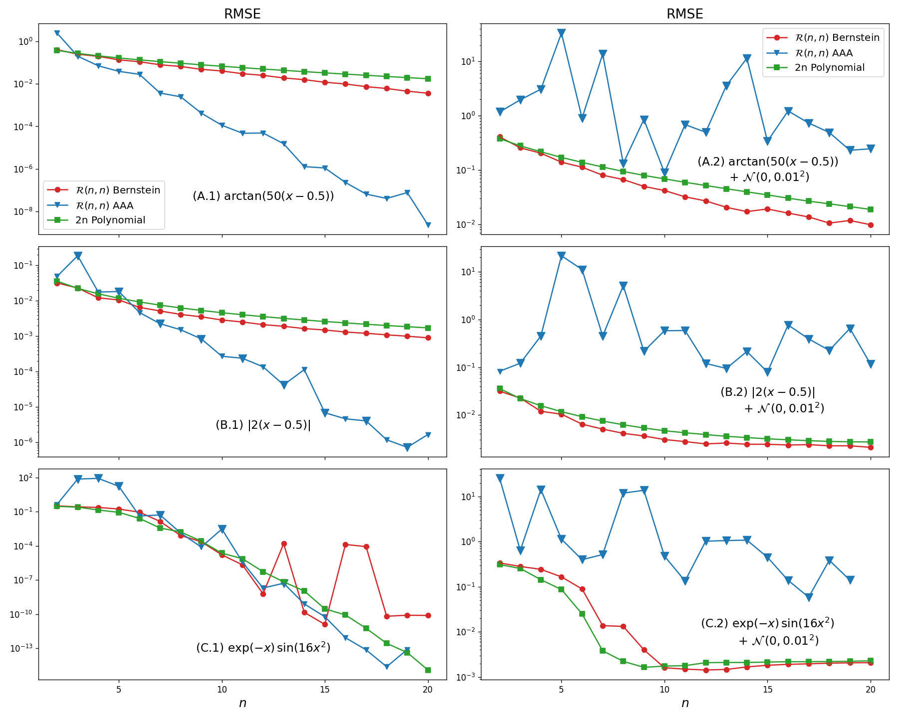
Figure 1: Numerical convergence of Polynomial, AAA (with cleanup on), and rational Bernstein Denominator fits on various functions with and without noise. For the functions in the left column, the data was generated using $\{i/1000,f(i/1000)\}_{0\leq i\leq 1000}$, while the right was data $\{(x_{j},f(x_{j})+\mathcal{N}(0,0.01^{2})\}_{1\leq j\leq 1000}$. The respective root mean squared error (RMSE) between the approximated function and the target function $f(x)$ at the sample points are shown. Thicker marker represents fits with poles inside the approximation interval $[0,1]$.

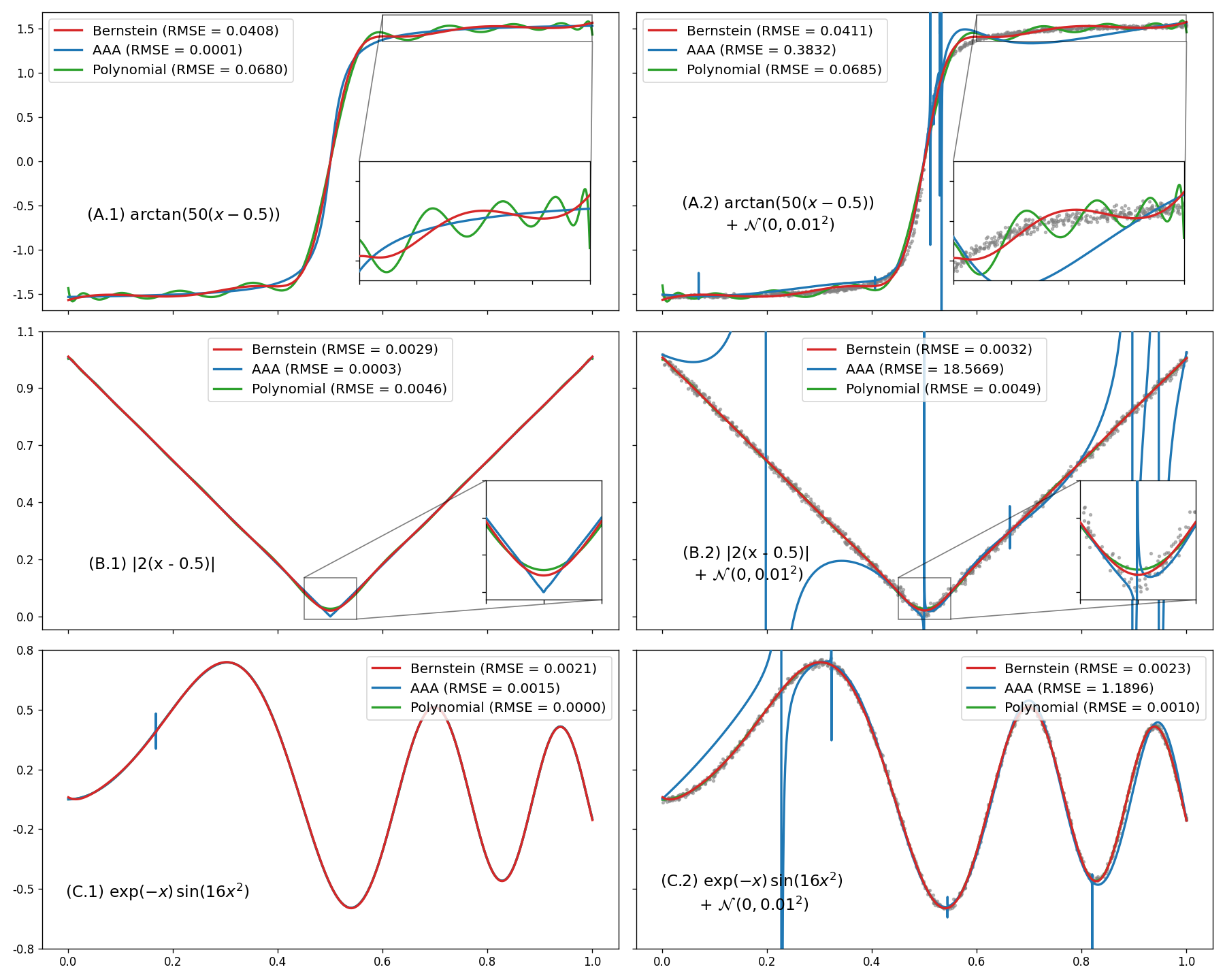
Figure 2: Approximations of various functions with and without noise using $\mathcal{R}(10,10)$ AAA (with cleanup on) and rational Bernstein Denominator algorithms, and a degree $20$ polynomial. For the functions in the left column, the data was generated using $\{i/1000,f(i/1000)\}_{0\leq i\leq 1000}$, while the right was data $\{(x_{j},f(x_{j})+\mathcal{N}(0,0.01^{2})\}_{1\leq j\leq 1000}$ with $x_{j}\sim U(0,1)$. The respective root mean squared error (RMSE) on the evaluation points are shown. Inside the interval $[0,1]$, the AAA algorithm (with cleanup on) exhibits six poles for (A.2), six poles for (B.2), and four poles for (C.2).

4.3 Quasiconvex vs Bernstein

We consider a more general setting with nonconstant noise to compare the Quasiconvex and rational Bernstein Denominator algorithms. Concretely, for the same functions, $\mathcal{F}=\{\arctan(50(x-0.5)),\ |2(x-0.5)|,\ \exp(-x)\sin(16x^{2})\}$, in the domain $[0,1]$, we generate the dataset $\{(x_{i},f(x_{i})+\mathcal{N}(0,(0.01+x_{i}/10)^{2})\}_{1\leq i\leq 1000}$ where $x_{i}\sim U(0,1)$ and all $f$ in $\mathcal{F}$. As a pedagogical example, we also look at the Wage dataset, which contains income survey data for men in the central Atlantic region of the USA [45].

For increasing values of $n$, we fit a $\mathcal{R}(n,n)$ Quasiconvex and rational Bernstein Denominator, as well as a $2n$ degree polynomial. As in Peiris et al. experiments, we take $\delta=0.1$ and $\zeta=50$ for the Quasiconvex algorithm, and we do not apply Sobolov-Smoothing, or hot-start to the rational Bernstein Denominator algorithm, and solve for the nonlinear residuals. The RMSE between the approximation and target function $f$ at the sample points $\{x_{i}\}_{i}$ is recorded for the simulated data for each fit. For the Wage dataset, since the true function is not known, we instead record the RMSE between the approximation function at $\{x_{i}\}_{i}$ and the corresponding target values $\{y_{i}\}_{i}$. Each fit was checked to see if it contained poles within the interval $[0,1]$. The results and examples of a $\mathcal{R}(10,10)$ Quasiconvex fit can be seen in Fig. 3.

Throughout all examples, the Quasiconvex algorithm consistently converges to a higher RMSE than the Bernstein Denominator and polynomial fit. This is perhaps due to the Quasiconvex algorithm minimizing the maximum instead of the l2-norm. Moreover, the Quasiconvex algorithm is still prone to producing approximations with poles in the interval $[0,1]$ and fits with spurious oscillations, as seen in its $\mathcal{R}(10,10)$ fit.

On the other hand, the rational Bernstein Denominator algorithm consistently produces fits with the lowest RMSE and minimal non-smooth artifacts than the respective polynomial fit. This is particularly prominent in the $\mathcal{R}(10,10)$ rational Bernstein Denominator and $20$-degree polynomial fits on the Wage dataset and the noisy $\arctan(50(x-0.5))$ function. On these datasets, the polynomial approximation consistently produces fast and large oscillations at the tail ends of the approximation interval, while the rational Bernstein Denominator is smooth at the tails. This is all performed while being free of poles inside $[0,1]$.

This shows the rational form’s strength in providing a great degree of explainability without oscillatory artifacts. But also highlights the necessity of the positivity enforced on the denominator through the Bernstein polynomials. Otherwise, poles will continually exist in the approximated function, as is the case with the Quasiconvex algorithm.

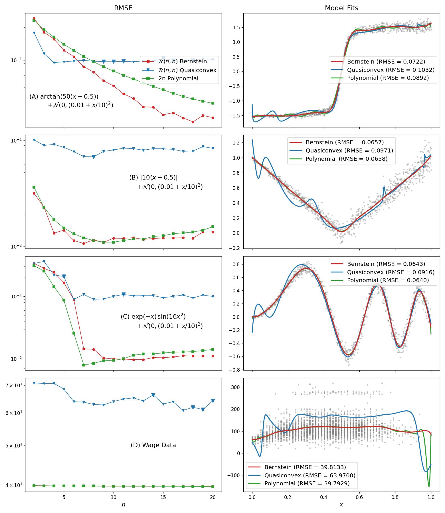
Figure 3: Comparisons of a $\mathcal{R}(n,n)$ Quasiconvex and rational Bernstein Denominator algorithm with a degree $2n$ polynomial, on noisy data. For the plots in the first three rows, the dataset is generated by $\{(x_{i},f(x_{i})+\mathcal{N}(0,(0.01+x_{i}/10)^{2}\}_{1\leq i\leq 1000}$ with $x_{i}\sim U(0,1)$, for various functions, $f$. The plot on the bottom row uses the Wage dataset [45]. For the plots on the left column, a $\mathcal{R}(n,n)$ Quasiconvex and rational Bernstein Denominator algorithm and a degree $2n$ polynomial were fit on the dataset with increasing values of $n$. The RMSE was recorded, and each fit was checked to see if poles inside $[0,1]$ existed. Thicker markers represent fits with poles inside the approximation interval $[0,1]$. On the right column, examples for $n=10$ for the three algorithms on the dataset corresponding to the left of the plot.

4.4 Smoothing Splines vs Bernstein

Smoothing splines are often a popular choice when modeling spatial data [50, 51, 52], as they provide the flexibility of high-degree polynomials without spurious oscillations. As such, we compare the Bernstein Denominator algorithm to smoothing splines in functions of two variables. In particular, we approximate the following functions inside the domain $[0,1]\times[0,1]$

$$f_{1}(x,z)=\sin[(4(x-0.5))^{2}+(4(z-0.5))^{2}],$$ (94)

$$f_{2}(x,z)=\sin(8x^{2})\sin(8z^{2}),$$ (95)

$$f_{3}(x,z)=\exp(4(x-0.5))\sin(4(z-0.5)).$$ (96)

We first compare the numerical convergence to these functions for increasing degrees of freedom on the noiseless dataset $\{(j/50,k/50,f_{i}(j/50,k/50)\}_{0\leq j,k\leq 50}$ for $i=1,2$ and $3$. In particular, for a given $n$, we take the Multivariate rational Bernstein Denominator to be degree $n$ in the $x$ and $z$ variable for the numerator and denominator, yielding $2(n+1)^{2}-1$ degrees of freedom. This is compared to a tensor product of penalized splines with $\Big{\lceil}\sqrt{2(n+1)^{2}-1}\Big{\rceil}$ basis splines in each variable, yielding $\Big{\lceil}\sqrt{2(n+1)^{2}-1}\Big{\rceil}^{2}+1$ free coefficients, including the constant term.

We apply hot-start and solve for the nonlinear residuals for the Multivariate rational Bernstein Denominator. The smoothing penalty for the Sobolov-Smoothed Multivariate rational Bernstein Denominator and the penalized spline is chosen through cross-validation over various values of smoothing strength. We record the RMSE between the approximation and the true function $f_{i}$ at the sample points $\{(j/50,k/50)\}_{j,k}$. The results are in Fig. 4.

Over the three examples in the noise-free case, the Sobolov-Smoothed rational Bernstein Denominator consistently has a faster numerical convergence rate than penalized splines. This again shows the benefits of using the rational form, as it provides significantly more explainability power than the corresponding penalized spline.

We now consider adding uniform Gaussian noise to our data, giving the altered dataset $\{(x_{j},z_{j},y_{j})\}_{1\leq j\leq 1000}$, where $x_{j}\sim U(0,1),z_{j}\sim U(0,1)$ and $y_{j}=f_{i}(x_{j},z_{j})+\mathcal{N}(0,0.1^{2})$. Two hundred replicate simulates of the dataset were made. We selected the smoothing penalty and the degree in the Multivariate rational Bernstein Denominator/degree of freedom for penalized splines using cross-validation on each replicate. We do not apply hot-start and solve for the nonlinear residuals for the Multivariate rational Bernstein Denominator. We compute the RMSE between the approximated function and the true function $f_{i}$ at each fit’s sample points $(x_{j},z_{j})$. The results are in Fig. 5.

On average, for all three functions, we see that the Sobolov-Smoothed rational Bernstein Denominator algorithm produces better fits than penalized splines. As such, although the rational Bernstein Denominator algorithm provides greater explainability power than penalized splines, it still does not flex itself to explain the noise in the dataset. Instead, it finds a smooth fit that approximates the true function well. This is mostly likely a result of the Sobolov-smoothing.

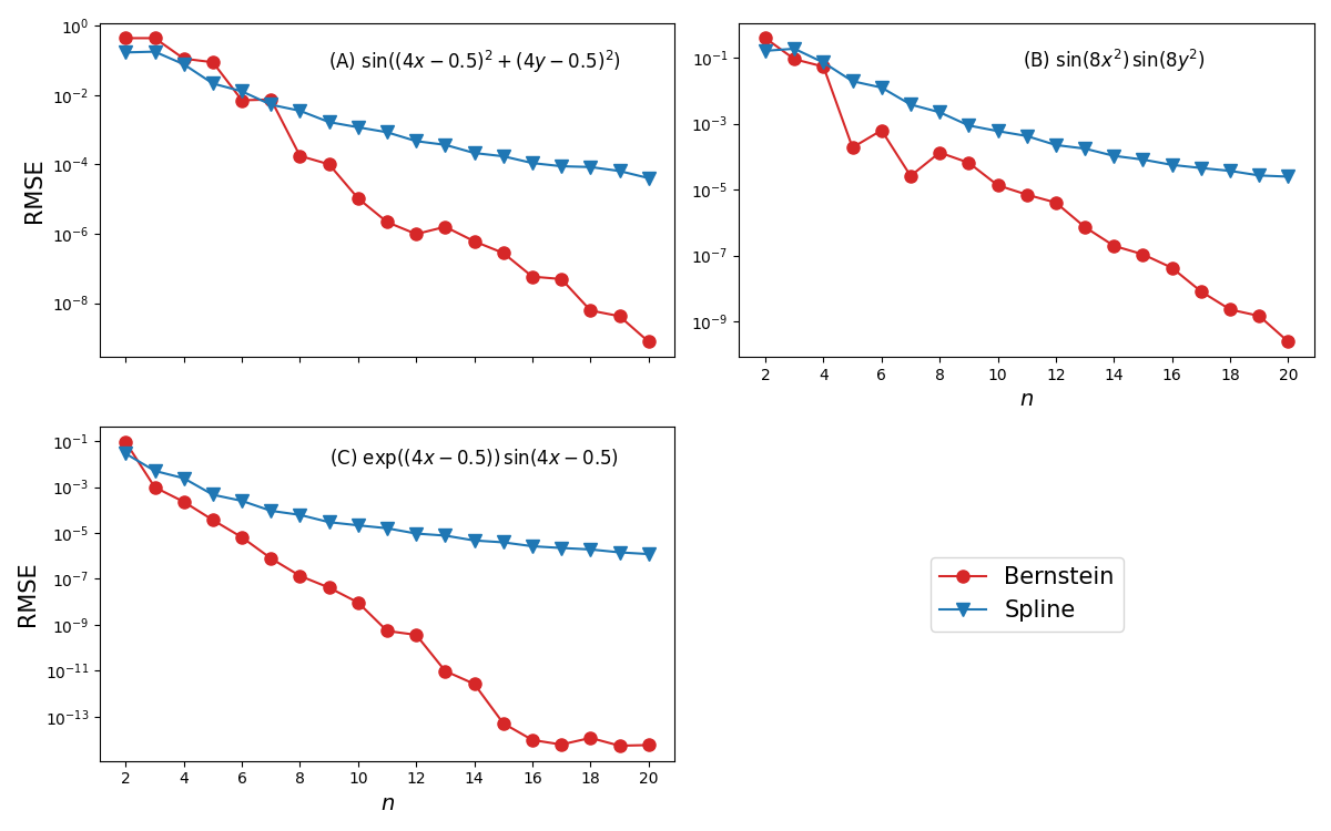
Figure 4: Numerical convergence on functions without noise for a Sobolov-Smoothed Multivariate rational Bernstein Denominator compared with a tensor product smoothing spline with an equivalent degree of freedom. For all plots, the dataset was generated by $\{(j/50,k/50,f(j/50,k/50)\}_{0\leq j,k\leq 5}$, for various functions, $f$. The RMSE between the fit and the function $f$ is recorded.

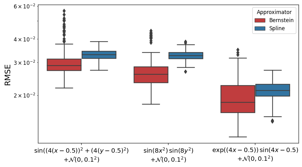
Figure 5: Comparisons of RMSE for Sobolov-Smoothed Multivariate rational Bernstein Denominator algorithm with tensor product smoothing splines. For all plots, the dataset was generated by $\{(x_{j},z_{j},f(x_{j},z_{j})+\mathcal{N}(0,0.1^{2})\}_{1\leq j\leq 1000}$, with $x_{j},z_{j}\sim U(0,1)$ for various functions, $f$. This plot shows the results after this dataset was generated 200 times for each function, with the RMSE between the fit and the true function, $f$, recorded.

5 Conclusion

Rational function approximation has been well-studied for functions without noise and is well-known to have better properties than polynomial approximation. However, few attempts have been made to guarantee pole-free approximations. Poles typically have been treated as a necessary by-product of rational functions, and the preventative measures to avert poles are methods to detect poles [43, 53] or attempt to stabilize the fit [35, 37].

The AAA algorithm [29], presented by the works of Nakatsukasa, Séte, and Trefethen, represents the current gold-standard method to perform rational function approximation. Indeed, we do not claim that our algorithm can beat the AAA algorithm overall. However, as the original AAA paper writes, "The fact is that the core AAA algorithm risks introducing unwanted poles when applied to problems involving real functions on real intervals". Moreover, a recent paper published in 2023 by Huybrechs and Trefethen [43] writes, "the appearance of unwanted poles in AAA approximants is not yet fully understood".

In this paper, we take an alternative route and put poles at the forefront of our method by guaranteeing rational polynomials with no poles in an interval on the real line. This is performed using the Bernstein polynomials and normalized coefficients to force strict positivity in the denominator. This represents a restricted class of rational functions and thus requires extra degrees of freedom to reach similar accuracy to traditional rational approximation methods. However, our method benefits from the compact representation and reduction in Runge’s phenomenon from rational functions while maintaining the stability given by polynomial approximation. Thus making our method particularly well suited for noisy data, a situation in which traditional rational approximation methods continually produce poles.

Our method typically takes longer than other rational or polynomial approximations, predominantly due to the iterative scheme. However, for our main application in differential equations, this cost pales compared to the typical runtime to numerically solve differential equations using spectral methods, which can take hours or days. Moreover, the compact representation afforded by the rational Bernstein Denominator algorithm can dramatically reduce the spectral methods’ runtime without any sacrifice to the solution’s accuracy.

Penalized splines are a popular method to perform function approximation on noisy data, as they similarly provide high degrees of flexibility while reducing Runge’s phenomenon. However, we find that our method significantly outperforms penalized splines on noiseless data and can beat penalized splines on noisy data. Our method also does this while being a $C^{\infty}[0,1]$ function, as opposed to penalized splines which are $C^{2}$ functions.

Paraphrasing the co-creator of the AAA algorithm, Llyod N. Trefethen, in his textbook on function approximation [54], there is no universally best approximation method. The AAA algorithm is best when one requires accurate estimations on data free of noise. We are not trying to replace it. However, when the dataset is noisy, or one wants to guarantee no poles inside the approximation interval reliably, we believe the Bernstein Denominator algorithm provides a promising and robust approach to using rational polynomials on data.

For further research, we’d like to look at theoretical guarantees on its convergence rate and better ways of introducing smoothing for rational function approximations. Bernstein polynomials also can be represented in Barycentric forms, which can perhaps lead to more stable ways of computing the rational function and potentially better approximations.

6 Acknowledgments

We thank Johnny Myungwon Lee for the helpful discussions on penalized splines.

References

- [1] G. Konidaris, S. Osentoski, and P. Thomas. Value function approximation in reinforcement learning using the fourier basis. Proceedings of the AAAI Conference on Artificial Intelligence, 25(1):380–385, August 2011.
- [2] Z. Zainuddin and O. Pauline. Function approximation using artificial neural networks. WSEAS Trans. Math., 7(6):333–338, June 2008.
- [3] Xuhui Meng and George Em Karniadakis. A composite neural network that learns from multi-fidelity data: Application to function approximation and inverse PDE problems. Journal of Computational Physics, 401:109020, January 2020.
- [4] Yeonjong Shin, Kailiang Wu, and Dongbin Xiu. Sequential function approximation with noisy data. Journal of Computational Physics, 371:363–381, October 2018.
- [5] P. Bader, S. Blanes, and F. Casas. Computing the matrix exponential with an optimized taylor polynomial approximation. Mathematics, 7(12):1174, December 2019.
- [6] James L Blue and Hermann K Gummel. Rational approximations to matrix exponential for systems of stiff differential equations. Journal of Computational Physics, 5(1):70–83, February 1970.
- [7] J. P. Boyd and J. R. Ong. Exponentially-convergent strategies for defeating the runge phenomenon for the approximation of non-periodic functions, part two: Multi-interval polynomial schemes and multidomain chebyshev interpolation. Applied Numerical Mathematics, 61(4):460–472, April 2011.
- [8] J. P. Boyd and L. F. Alfaro. Hermite function interpolation on a finite uniform grid: Defeating the runge phenomenon and replacing radial basis functions. Applied Mathematics Letters, 26(10):995–997, October 2013.
- [9] John P. Boyd. Trouble with gegenbauer reconstruction for defeating gibbs’ phenomenon: Runge phenomenon in the diagonal limit of gegenbauer polynomial approximations. Journal of Computational Physics, 204(1):253–264, March 2005.
- [10] J. P. Boyd. Chebyshev and Fourier Spectral Methods. Dover Books on Mathematics. Dover Publications, Mineola, NY, second edition, 2001.
- [11] T. A. Driscoll, F. Bornemann, and L. N. Trefethen. The chebop system for automatic solution of differential equations. BIT Numerical Mathematics, 48(4):701–723, November 2008.
- [12] A. Karageorghis and T. N. Phillips. Chebyshev spectral collocation methods for laminar flow through a channel contraction. Journal of Computational Physics, 84(1):114–133, September 1989.
- [13] S. Olver and A. Townsend. A fast and well-conditioned spectral method. SIAM Review, 55(3):462–489, January 2013.
- [14] K. J. Burns, G. M. Vasil, J. S. Oishi, D. Lecoanet, and B. P. Brown. Dedalus: A flexible framework for numerical simulations with spectral methods. Physical Review Research, 2(2), April 2020.
- [15] G. M. Vasil, K. J. Burns, D. Lecoanet, S. Olver, B. P. Brown, and J. S. Oishi. Tensor calculus in polar coordinates using jacobi polynomials. Journal of Computational Physics, 325:53–73, November 2016.
- [16] G. M. Vasil, D. Lecoanet, K. J. Burns, J. S. Oishi, and B. P. Brown. Tensor calculus in spherical coordinates using jacobi polynomials. part-i: Mathematical analysis and derivations. Journal of Computational Physics: X, 3:100013, June 2019.
- [17] D. Lecoanet, G. M. Vasil, K. J. Burns, B. P. Brown, and J. S. Oishi. Tensor calculus in spherical coordinates using jacobi polynomials. part-II: Implementation and examples. Journal of Computational Physics: X, 3:100012, June 2019.
- [18] I. P. A. Papadopoulos, T. S. Gutleb, R. M. Slevinsky, and S. Olver. Building hierarchies of semiclassical jacobi polynomials for spectral methods in annuli, 2023.
- [19] S. Olver, A. Townsend, and G. M. Vasil. A sparse spectral method on triangles. SIAM Journal on Scientific Computing, 41(6):A3728–A3756, January 2019.
- [20] S. Olver, A. Townsend, and G. M. Vasil. Recurrence relations for a family of orthogonal polynomials on a triangle. In Lecture Notes in Computational Science and Engineering, pages 79–92. Springer International Publishing, 2020.
- [21] A. C. Ellison, K. Julien, and G. M. Vasil. A gyroscopic polynomial basis in the sphere. Journal of Computational Physics, 460:111170, July 2022.
- [22] S. Olver, R. M. Slevinsky, and A. Townsend. Fast algorithms using orthogonal polynomials. Acta Numerica, 29:573–699, May 2020.
- [23] K. J. Burns, D. Fortunato, K. Julien, and G. M. Vasil. Corner cases of the generalized tau method, 2022.
- [24] A. Townsend and S. Olver. The automatic solution of partial differential equations using a global spectral method. Journal of Computational Physics, 299:106–123, October 2015.
- [25] V. Peiris, N. Sharon, N. Sukhorukova, and J. Ugon. Generalised rational approximation and its application to improve deep learning classifiers. Applied Mathematics and Computation, 389:125560, January 2021.
- [26] M. S. Floater and K. Hormann. Barycentric rational interpolation with no poles and high rates of approximation. Numerische Mathematik, 107(2):315–331, June 2007.
- [27] P. Gonnet, R. Pachon, and L. N. Trefethen. Robust rational interpolation and least-squares. Electronic Transactions on Numerical Analysis, 38:146–167, 2011.
- [28] J. P. Berrut. Rational functions for guaranteed and experimentally well-conditioned global interpolation. Computers & Mathematics with Applications, 15(1):1–16, 1988.
- [29] Y. Nakatsukasa, O. Sète, and L. N. Trefethen. The AAA algorithm for rational approximation. SIAM Journal on Scientific Computing, 40(3):A1494–A1522, January 2018.
- [30] Y. Nakatsukasa and L. N. Trefethen. An algorithm for real and complex rational minimax approximation. SIAM Journal on Scientific Computing, 42(5):A3157–A3179, January 2020.
- [31] S. L. Filip, Y. Nakatsukasa, L. N. Trefethen, and B. Beckermann. Rational minimax approximation via adaptive barycentric representations. SIAM Journal on Scientific Computing, 40(4):A2427–A2455, January 2018.
- [32] J. P. Berrut and G. Klein. Recent advances in linear barycentric rational interpolation. Journal of Computational and Applied Mathematics, 259:95–107, March 2014.
- [33] R. Pachón and L. N. Trefethen. Barycentric-remez algorithms for best polynomial approximation in the chebfun system. BIT Numerical Mathematics, 49(4):721–741, October 2009.
- [34] C. Sanathanan and J. Koerner. Transfer function synthesis as a ratio of two complex polynomials. IEEE Transactions on Automatic Control, 8(1):56–58, January 1963.
- [35] J. M. Hokanson. Multivariate rational approximation using a stabilized sanathanan-koerner iteration, 2020.
- [36] V. Peiris, N. Sharon, N. Sukhorukova, and J. Ugon. Generalised rational approximation and its application to improve deep learning classifiers. Applied Mathematics and Computation, 389, January 2021.
- [37] P. Gonnet, S. Güttel, and L. N. Trefethen. Robust padé approximation via SVD. SIAM Review, 55(1):101–117, January 2013.
- [38] G. A. Baker and P. Graves-Morris. Padé’ Approximants. Encyclopedia of Mathematics and its Applications. Cambridge University Press, 2 edition, 1996.
- [39] A. V. Ferris-Prabhu and D. H. Withers. Numerical analytic continuation using padé approximants. Journal of Computational Physics, 13(1):94–99, September 1973.
- [40] S. Bernstein. Démonstration du théorème de weierstrass fondée sur le calcul des probabilités (demonstration of a theorem of weierstrass based on the calculus of probabilities). Communications of the Kharkov Mathematical Society, 13:1–2, 1912.
- [41] G. M. Phillips. Bernstein polynomials. In CMS Books in Mathematics, chapter 7, pages 247–290. Springer New York, 2003.
- [42] J.M. McNamee. Chapter 6 - matrix methods. In J.M. McNamee, editor, Numerical Methods for Roots of Polynomials, Part I, volume 14 of Studies in Computational Mathematics, pages 207–321. Elsevier, 2007.
- [43] D. Huybrechs and L. N. Trefethen. AAA interpolation of equispaced data. BIT Numerical Mathematics, 63(2), March 2023.
- [44] D. P. Williamson and D. B. Shmoys. Greedy Algorithms and Local Search, page 27–56. Cambridge University Press, 2011.
- [45] G. James, D. Witten, T. Hastie, and R. Tibshirani. An Introduction to Statistical Learning. Springer US, 2021.
- [46] R. Beals and R. Wong. The classical orthogonal polynomials. Cambridge Studies in Advanced Mathematics. Cambridge University Press, 2016.
- [47] G. Chi and J. Zhu. Spatial Regression Models for the Social Sciences. SAGE Publications, Inc., 2020.
- [48] J. Chok and G. M. Vasil. Convex optimization over a probability simplex, 2023.
- [49] D. Lecoanet and E. Quataert. Internal gravity wave excitation by turbulent convection. Monthly Notices of the Royal Astronomical Society, 430(3):2363–2376, February 2013.
- [50] S. N. Wood. Low-rank scale-invariant tensor product smooths for generalized additive mixed models. Biometrics, 62(4):1025–1036, May 2006.
- [51] P. H.C. Eilers, I. D. Currie, and M. Durbán. Fast and compact smoothing on large multidimensional grids. Computational Statistics & Data Analysis, 50(1):61–76, January 2006.
- [52] M. X. Rodríguez-Álvarez, D.-J. Lee, T. Kneib, M. Durbán, and P. Eilers. Fast smoothing parameter separation in multidimensional generalized p-splines: the SAP algorithm. Statistics and Computing, 25(5):941–957, April 2014.
- [53] T. Driscoll, Y. Nakatsukasa, and L. N. Trefethen. AAA rational approximation on a continuum, 2023.
- [54] L. N. Trefethen. Approximation Theory and Approximation Practice, Extended Edition. Society for Industrial and Applied Mathematics, January 2019.