Entanglement entropy in a time-dependent holographic Schwinger pair creation

Abstract

We analyze the entanglement of a Schwinger pair created by a time-dependent pulse. In the semiclassical approximation, the pair creation by a pulse of external electric field is captured by a periodic worldline instanton. At strong gauge coupling, the gauge-gravity dual worldsheet instanton exhibits a falling wormhole in AdS. We identify the tunneling time at the boundary with the inverse Unruh temperature, and derive the pertinent entanglement entropy between the created pair using thermodynamics. The entanglement entropy is enhanced by the sub-barrier tunneling process, and partly depleted by the radiation in the post-barrier process.

I Introduction

Schwinger pair creation Schwinger (1951) is a quantum process in which a pair of particles is produced from the vacuum in an external electric field. In quantum chromodynamics (QCD), the external chromoelectric field inside a confining string can lead to the production of a quark-antiquark pair, leading to string breaking when the string energy exceeds the light meson mass. This process is used in event generators (such as Lund and PYTHIA) Andersson et al. (1983) to account for jet fragmentation in high energy collisions  Buskulic et al. (1995).

The pair creation proceeds through tunneling, a quintessential quantum process. The vacuum pair tunnels through a potential barrier under the effect of a strong background field, and is produced with a finite probability. Throughout the creation process, the pair is correlated and interacts with both with the external (classical) field and the quantum gauge field. Quantum entanglement is the measure of these correlations throughout the pair history.

Recently, this pair creation process was used as an illustration of the Einstein-Rosen-Podolsky (EPR) paradox, in the context of quantum field theory at strong coupling Jensen and Karch (2013); Sonner (2013). In this strong coupling regime, the gravity dual of the pair is a string worldsheet Gorsky et al. (2002); Xiao (2008); Semenoff and Zarembo (2011); Lewkowycz and Maldacena (2014); Chernicoff et al. (2013); Jensen et al. (2014); Hubeny and Semenoff (2014); Ghodrati (2015); Semenoff (2018); Yeh (2023) with a non-traversable wormhole, or Einstein-Rosen (ER) bridge Jensen and Karch (2013). The quantum entanglement entropy of the pair is sensitive to the location of the ER bridge Jensen and Karch (2013); Maldacena and Susskind (2013).

In the receding quark-antiquark pair in Schwinger process, the end-points of the string are never causally connected. However the pair is entangled owing to its color neutrality. In non-confining dual gravity description, the entanglement entropy was found to be of order $\sqrt{\lambda}$ in the weak field limit Jensen and Karch (2013); Hubeny and Semenoff (2014, 2014); Grieninger et al. (2023); Hubeny and Semenoff (2015), with $\lambda=g_{Y}^{2}N_{c}$ the strong ^′t Hooft coupling. In this work, we will extend our discussion which was restricted to static electric fields Grieninger et al. (2023) and explore the entanglement in the pair creation process in the presence of a time-dependent electric pulse.

In QCD, a strong gauge field pulse could be generated by a highly boosted nucleus, assuming that all wee partons in the nuclear wavefunction add up coherently, see  Gelis et al. (2010); Kovchegov and Levin (2013) and references therein. In the rest frame of a target interacting with this highly boosted nucleus, the target is crossed by a “gluon wall" Bjorken (1992) that is a pulse of gauge field. This pulse will lead to pair creation. The entanglement entropy of the pair can be converted to the Gibbs entropy of the final hadronic state. For QED, the equality between the entanglement and Gibbs entropies in Schwinger pair production by a pulse was demonstrated in Florio and Kharzeev (2021). For CFTs it was shown in Casini et al. (2011) that the entanglement entropy across a spherical region is equal to the thermal entropy of the hyperbolic geometry $\mathbb{R}\times\mathbb{H}^{d-1}$, which is the direct product of time and the hyperbolic plane. In QCD, the effects of confinement have to be taken into account compared to the weak coupling QED calculation in Florio and Kharzeev (2021), as well as radiation in the final state. Our present work addresses this problem from a holographic perspective.

The organization of the paper is as follows: In section II we briefly review the semiclassical analysis of the Schwinger process for particle pair creation by a pulse. The worldline instanton solution is discussed, and an estimate of its entanglement entropy is given. In section III, we extend the analysis to strong coupling, where the dual of the worldline is a worldsheet in AdS. The worldsheet is characterized by a moving wormhole, a hallmark of the time-varying pulse at the boundary. We show that the entanglement entropy receives a positive contribution from tunneling (sub-barrier process) and a negative contribution from radiation loss (post-barrier process). Our conclusions are in section V.

II Tunneling in a time-dependent external field

Consider first a scalar particle of mass $M$, in an Abelianized external field moving in proper time, with the action

$$S=\int d\tau M\sqrt{\dot{x}^{2}}+i\oint A.$$ (1)

Tunneling in (1) is captured by the worldline instanton solution to the classical equations of motion in Euclidean signature,

$$M\frac{d}{d\tau}\bigg{(}\frac{{\dot{x}_{\mu}}}{\sqrt{\dot{x}^{2}}}\bigg{)}=iF_{\mu\nu}\dot{x}_{\nu}.$$ (2)

For a time dependent pulse electric field in Minkowski signature,

$$E(t)=\frac{E}{{\rm cosh}^{2}(\omega t)}$$ (3)

the Euclideanized vector potential in (1)

$$A_{3}(x_{4})=\frac{-iE}{\omega}{\rm tan}(\omega x_{4})$$ (4)

is purely imaginary. Since (4) is singular for $x_{4S}=\frac{\pi}{2\omega}$, all worldlines are bounded by this maximum value in $|x_{4}|\leq x_{4S}$.

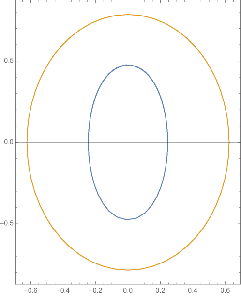
Figure 1: Contour plot of (7) for $a=\gamma=1$ (outer) and $a=1,\gamma=2.5$ (inner) with $M=1$.

II.1 Worldline instanton

The tunneling process was discussed by many Brezin and Itzykson (1970); Popov (1971); Kim and Page (2002); Dunne and Schubert (2005); Kharzeev and Tuchin (2005); Gies and Klingmuller (2005); Gies and Torgrimsson (2016, 2017), with the instanton solution given by Dunne and Schubert (2005)

$$x_{3}(\tau)=\frac{1}{a\gamma}\frac{1}{\sqrt{1+{\gamma}^{2}}}{\rm arcsinh}\bigg{(}\gamma{\rm cos}\bigg{(}a\sqrt{1+\gamma^{2}}\tau\bigg{)}\bigg{)}\equiv\frac{1}{a\bar{\gamma}}{\rm sinh}^{-1}(\gamma{\rm cos}(\bar{a}\tau)),$$

$$x_{4}(\tau)=\frac{1}{a\gamma}{\rm arcsin}\bigg{(}\frac{\gamma}{\sqrt{1+{\gamma}^{2}}}{\rm sin}\bigg{(}a\sqrt{1+\gamma^{2}}\tau\bigg{)}\bigg{)}\,\,\,\,\,\,\,\,\equiv\frac{1}{a\gamma}{\rm sin}^{-1}(\underline{\gamma}{\rm sin}(\bar{a}\tau)).$$ (5)

It is periodic, with period

$$\beta=\frac{2\pi}{\bar{a}}\equiv\frac{2\pi}{a\sqrt{1+\gamma^{2}}}$$ (6)

with $a=E/M$ and $\gamma=\omega/a$. Throughout, $E\equiv g_{Y}E$ refers to the invariant electric field in the probe D3 brane. Eqs (II.1) describe a cyclotron-like trajectory that satisfies $\dot{x}_{3}^{2}+\dot{x}_{4}^{2}=1$, since the applied force in (2) is magnetic in Euclidean signature. The Wilson loop traced by the boundary worldline (II.1) is elliptic-like in general,

$$\frac{{\rm sh^{2}}(a\bar{\gamma}x_{3})}{\gamma^{2}}+\frac{{\rm sin^{2}}(a\gamma x_{4})}{\underline{\gamma}^{2}}=1$$ (7)

as illustrated in Fig. 1. The high eccentricity of the trajectories along the $x_{4}$ direction follows from the singularity of the force from the pulse, at $x_{4S}=\frac{\pi}{2\omega}$ of (1) noted earlier. It becomes circular in the static limit, $x_{3}^{2}+x_{4}^{2}\rightarrow\frac{1}{a^{2}}$ as $\omega\rightarrow 0$.

II.2 Particle entanglement

For scalar pair creation of mass $2M$, the action evaluated using (II.1) is

$$S(\beta)=\frac{\beta M}{1+(1-(\beta\omega/2\pi)^{2})^{\frac{1}{2}}}$$ (8)

with $e^{-2S(\beta)}$, the penalty for tunneling in the absence of confinement. When the pulse is about static, $S(\beta)\sim\frac{1}{2}\beta M$ in agreement with Schwinger^′ original result. Alternatively, when the pulse is very sharp in time, $S(\beta)\sim\frac{2\pi M}{\omega}$. At large frequency, the pair production is uninhibited.

We interpret (8) as the free energy $S(\beta)=\beta F(\beta)$ of the tunneling pair in the pulse. As a result, the corresponding quantum entropy at the boundary, is given by thermodynamics

$$S^{B}_{EE}= \frac{\beta M\gamma^{2}}{(1+\sqrt{1+\gamma^{2}})^{2}}.$$ (9)

It vanishes in the static limit as $S_{EE}^{B}\sim\beta M\gamma^{2}$, and for large frequencies vanishes as $S_{EE}^{B}\sim\frac{2\pi M}{\omega}$.

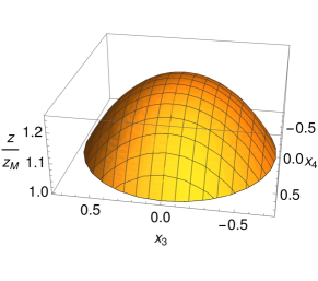
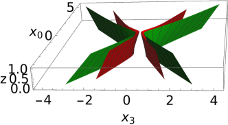
Figure 2: Left: Sub-barrier Euclidean string worldsheet, for pair production in a pulse for $z_{M}E=0.44$ and $z_{M}\omega=0.25$. Right: Post-barrier Minkowski string worldsheet, for pair production in a pulse, for $\gamma=a=1$ (green) and $\gamma=2,a=1$ (red), with $z_{M}=0$.

III Holographic pair production

The worldline instanton (II.1) captures the pair production of a particle of mass $M$ at the boundary, at weak coupling. In the double limit of strong ^′t Hooft coupling $\lambda$ and large $N_{c}$, the gravity dual description is captured by a string worldsheet sourced by the boundary Wilson loop on a D3 brane. Holographic pair production of particles as end points of strings, extends (1) to the Nambu-Goto action in bulk

$$S=\sigma_{T}\int\mathrm{d}\tau\,\mathrm{d}\sigma|{\rm det}g_{MN}\,\partial_{\tau}X^{M}\partial_{\sigma}X^{N}|^{\frac{1}{2}}+i\oint A$$

in AdS₅ with line element

$$\mathrm{d}s^{2}=g_{MN}\mathrm{d}x^{M}\mathrm{d}x^{N}=\frac{L^{2}}{z^{2}}(\mathrm{d}x_{\mu}^{2}+\mathrm{d}z^{2})$$ (11)

with $\sigma_{T}L^{2}=\sqrt{\lambda}/2\pi$. The coordinate embedding of the string $X^{M}(\tau,\sigma)$ can be obtained numerically in Euclidean signature, using the Nambu-Goto action for the string in bulk, as constrained by the Wilson loop at the D3 boundary.

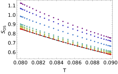
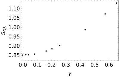
Figure 3: Left: On-shell action vs $T=1/\beta$ for different $\omega$ (increasing from red to purple). The analytical result for $\omega=0$ is the black dashed line. Right: On-shell action vs $\gamma$ for $T=0.08$ and $\lambda=12$.

III.1 Euclidean string worldsheet

In Euclidean signature, the worldsheet surface in bulk is ellipsoidal. To parametrize it in AdS₅, we use cylindrical coordinates $r,\varphi,z$,

$$x^{M}\!(z,\varphi)\!=\!(0,0,r(z,\varphi){\rm cos}(\varphi),r(z,\varphi){\rm sin}(\varphi),z)$$ (12)

in terms of which the Nambu-Goto action plus the electric field at the boundary, read

$$S=\frac{\sqrt{\lambda}}{2\pi}\int_{z_{M}}^{z_{E}}\mathrm{d}z\int_{0}^{2\pi}\mathrm{d}\varphi\,\frac{1}{z^{2}}\bigg{(}r^{2}(1+r_{z}^{2})+r_{\varphi}^{2}\bigg{)}^{\frac{1}{2}}+i\oint A$$ (13)

with the shorthand notation $r_{z}=\partial_{z}r$ and $r_{\varphi}=\partial_{\varphi}r$. Here $z_{M}$ is the position of the probe D3 brane, with $z_{M}=\frac{\sqrt{\lambda}}{2\pi M}$ fixed by the mass of the probe D3 brane at the boundary. Here $z_{E}$ is the tip (extrema) of the ellipsoidal-like worldsheet in bulk,

$$r(z_{E},\varphi)=0\qquad r_{z}(z_{E},\varphi)=\infty.$$ (14)

In (13) we have used the fact that the electric field (II.1) acts as a magnetic field in Euclidean signature, with the "vector potential" (4). Its contribution to the Wilson loop at the boundary $z=z_{M}$, is

$$i\oint A=\int_{0}^{2\pi}\mathrm{d}\varphi\frac{E}{\omega}{\rm tan}(\omega r{\rm sin}\varphi)({\rm cos}\varphi r_{\varphi}-r{\rm sin}\varphi).$$

The bulk equation of motion follows by variation

$$-rr_{zz}(r^{2}+r_{\varphi}^{2})+rr_{\varphi\varphi}(1+r_{z}^{2})$$

$$-\frac{2}{z}r_{\varphi}(r^{2}(1+r_{z}^{2})+r_{\varphi}^{2})$$

$$-r^{2}r_{z}^{2}-2r_{\varphi}^{2}-2rr_{z}r_{\varphi}r_{z\varphi}-r^{2}=0$$ (16)

subject to the Lorentz force along the z-direction at the D3 brane on the boundary at $z=z_{M}$,

$$\frac{\sqrt{\lambda}}{2\pi}\frac{1}{z_{M}^{2}}\frac{r^{2}r_{z}}{(r^{2}(1+r_{z}^{2})+r_{\varphi}^{2})^{\frac{1}{2}}}$$

$$=\frac{E}{{\rm cos}^{2}(\omega r{\rm sin}\varphi)}\bigg{(}r-\frac{1}{2}r_{\varphi}\,{\rm sin}{2\varphi}\bigg{)}.$$ (17)

Again, we made use of the short hand notations $r_{zz}=\partial_{z}^{2}r$, $r_{\varphi\varphi}=\partial_{\varphi}^{2}r$, and $r_{z\varphi}=\partial_{z}\partial_{\varphi}r$. (III.1) subject to the boundary condition (17) can be solved numerically using the pseudo-spectral methods (with Chebychev discretization in the radial direction and Fourier discretization in $\varphi$).

In Fig. 2 (left) we show the Euclidean surface for $z_{M}E=0.44$ and $z_{M}\omega=0.25$. The on-shell action $S_{OS}$ of the ellipsoidal surface (13), sets the tunneling probability for the holographic pair production in the pulse, in the strong field limit. In Fig. 3 (left) we show the behavior of the on-shell action versus $T=1/\beta$ given in (6), for increasing frequencies of the pulse from bottom-red to top-purple. The numerical results shown in the dashed-black curve for $\omega=0$, coincide with the analytical results for the holographic pair production derived in Semenoff and Zarembo (2011)

$$S_{OS}\rightarrow\frac{\sqrt{\lambda}}{2}\bigg{(}\sqrt{\frac{T_{c}}{T}}-\sqrt{\frac{T}{T_{c}}}\bigg{)}^{2}$$ (18)

with

$$T_{c}=\frac{a_{c}}{2\pi}=\frac{1}{2\pi}\frac{1}{\sqrt{R^{2}+z_{M}^{2}}}.$$

Our numerical results, generalize (28) to a time-dependent pulse.

In Fig. 3 (right) we show the on-shell action versus $\gamma=M\omega/E$ for fixed temperature. The increasing action reflects on the larger penalty for the pair production rate, with larger $\omega$ and fixed $E$ as the pulse is short lived. Equivalently, the larger $E$ for fixed $\omega$, the smaller the penalty for pair production.

III.2 Particle multiplicities in a pulse

Strong and coherent chromo-electric pulses can be produced during the initial phase of an ultra-relativistic heavy-ion collision. The higher the energy of the ion projectile, the stronger the field and the shorter is its duration in the frame of the target.

Strong chromo-electric fields can produce light quark pairs through the Schwinger mechanism. For the strongly coupled phase, the mean number of produced pairs in the pulse is

$$\bar{n}\!=\!\sum_{n=1}^{\infty}n\,p_{n}\!=\!\sum_{n=1}^{\infty}n\,(e^{S_{OS}}\!-1)\,e^{-nS_{OS}}\!=\!\frac{1}{1-e^{-S_{OS}}}.$$

In Fig. 4, we show the dependence of the mean number of produced particles on $\gamma=M\frac{\omega}{E}$ (not to be confused with the Lorentz contraction factor). The mean number of produced pairs decreases with increasing $\gamma$, since tunnelling is more suppressed (note that the case of strong and static electric fields corresponds to $\gamma\to 0$.)

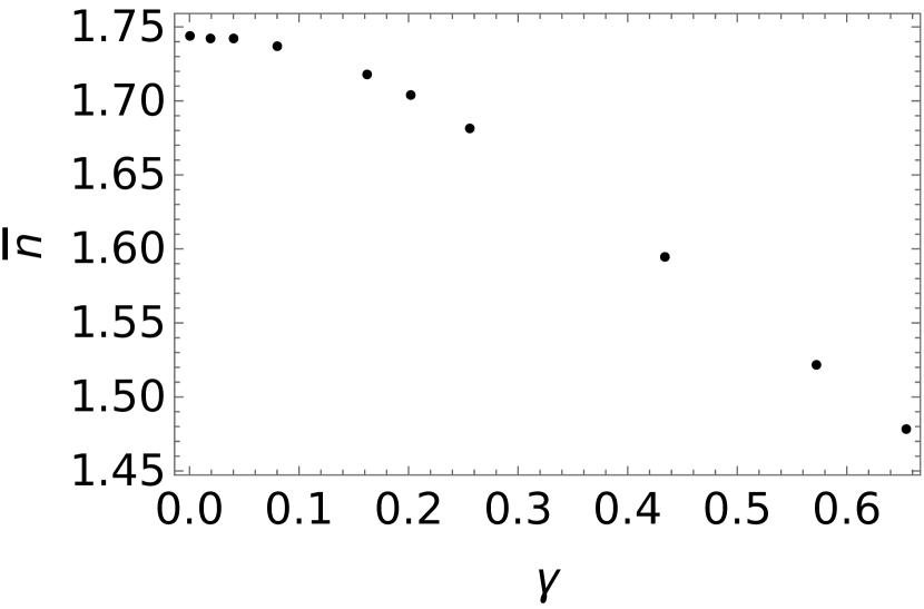
Figure 4: Mean number of particles produced in the pulse as a function of $\gamma=M\frac{\omega}{E}$ for $T=0.08$, $z_{M}=1$ and $\lambda=12$.

III.3 Minkowski string worldsheet

In Minkowski signature, the worldsheet in bulk is the locus of the retarded radiation, sourced by an accelerating $q\bar{q}$ pair tracing the Wilson loop with hyperbolic-like worldlines. It follows from the ruled surface in bulk Mikhailov (2003)

$$X^{M}(t,z)=(z\dot{x}^{\mu}(t)+x^{\mu}(t),z)$$ (19)

with $\sigma=z$. The boundary worldlines

$$x^{\mu}(t)=(x^{0}(t),0,0,x^{3}(t))$$

follow from (II.1) by analytical continuation $\tau\rightarrow it$ and $ix_{4}\rightarrow x_{0}$,

$$x^{3}(t)=\frac{1}{a\bar{\gamma}}{\rm sinh}^{-1}(\gamma{\rm cosh}(\bar{a}t))$$

$$x^{0}(t)=\frac{1}{a\gamma}{\rm sinh}^{-1}(\underline{\gamma}{\rm sinh}(\bar{a}t))$$ (20)

with $\dot{x}^{2}_{\mu}=-1$. In Fig. 2 (right) we show two worldsheets as given by (19) and traced by (III.3) with $\gamma=a=1$ (green) and $\gamma=2,a=1$ (red). We have set $z_{M}=0$ for the D3 brane for convenience. For $\gamma=0$, the ruled surface (right) is the analytical continuation of the Euclidean surface (left), as initially observed in Jensen and Karch (2013); Sonner (2013).

III.4 Moving wormhole on the worldsheet

The time-dependent string worldsheet harbors a moving wormhole. To see this, consider the line element associated to (19)

$$\mathrm{d}X_{M}^{2}=\left(a^{2}(t)-\frac{1}{z^{2}}\right)\mathrm{d}t^{2}-\frac{2}{z^{2}}\mathrm{d}t\,\mathrm{d}z$$ (21)

with a squared acceleration

$$a^{2}(t)\equiv\ddot{x}^{2}=a^{2}\bigg{(}1+\underline{\gamma}^{2}{\rm sinh}^{2}(\bar{a}t)\bigg{)}^{-2}$$ (22)

and an effective horizon at $z_{H}(t)=1/a(t)$. In the static limit $\omega\rightarrow 0$, it reduces to the static horizon $z_{H}\rightarrow\frac{1}{a}$. Away from the static limit, the horizon is moving away from the boundary, with asymptotically

$$z_{H}(t)\sim\frac{\gamma\underline{\gamma}}{4{\overline{a}}}\,e^{2\overline{a}t}.$$ (23)

The black hole is falling rapidly in bulk, a hallmark of a time-dependent problem Shuryak et al. (2007); Kim et al. (2008); Grieninger and Zahed (2023).

IV Entanglement for the pulsing string

The effective horizon $z_{H}(t)$ splits the worldsheet in bulk into a causal part with $z<z_{H}(t)$ and a non-causal part with $z>z_{H}(t)$. This is also the location of a time-dependent wormhole, as observed in Jensen and Karch (2013) for the static case.

The entanglement entropy (EE) receives contribution from both the causal part of the worldsheet (positive) and non-causal part of the worldsheet (negative). We will distinguish between the weak field limit and strong coupling where the worldsheet surface can be obtained both analytically and numerically (for the causal part only), and the strong field and strong coupling limit where the worldsheet surface can only be obtained numerically.

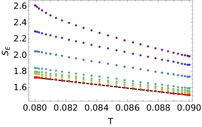
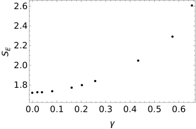
Figure 5: Left: Entanglement entropy as a function of the temperature $T=1/\beta$ for different $\omega$ (increasing from red to purple). The analytical result for $\omega=0$ is the black dashed line. Right: Entanglement entropy as a function of $\gamma=\omega/a$ for $T=0.08$, $z_{M}=1$ and $\lambda=12$.

IV.1 Causal contribution to EE:
Weak field limit

The causal contribution to the entanglement entropy in the weak field limit and finite $\gamma=M\omega/E$ is given numerically by the Euclidean surface, and more explicitly by the ruled surface in Minkowski signature, as we have discussed in Grieninger et al. (2023). Specifically, the causal contribution of the worldsheet action

$$S^{C}= 2\times\frac{\sqrt{\lambda}}{2\pi}\int_{-\frac{1}{2}{\cal T}}^{+\frac{1}{2}{\cal T}}\mathrm{d}t\int_{z_{M}}^{\frac{1}{a(t)}}\frac{\mathrm{d}z}{z^{2}}$$

$$= 2\times\frac{\sqrt{\lambda}}{2\pi}\int_{-\frac{1}{2}{\cal T}}^{+\frac{1}{2}{\cal T}}\mathrm{d}t\bigg{(}\frac{1}{z_{M}}-a(t)\bigg{)}.$$ (24)

The first contribution (from the minuend in (24)) reduces to the rest mass contribution

$$S_{(1)}^{C}=\frac{\sqrt{\lambda}}{\pi\,z_{M}}\int_{-\frac{1}{2}{\cal T}}^{+\frac{1}{2}{\cal T}}\!\!\mathrm{d}t=2\times\,{\cal T}\,\frac{\sqrt{\lambda}}{2\pi z_{M}}=2{\cal T}M.$$ (25)

For $\omega\neq 0$, the time integration of the subtracted term in (24) gives

$$S_{(2)}^{C}=-\frac{\sqrt{\lambda}}{\pi}\int_{-\frac{1}{2}{\cal T}}^{+\frac{1}{2}{\cal T}}\mathrm{d}t\,a(t)=2\times\frac{\sqrt{\lambda}}{2\pi}\,{\rm ln}\left|\frac{\left(\sqrt{1+\gamma^{2}}+1\right)e^{-\bar{a}{\cal T}}+\sqrt{1+\gamma^{2}}-1}{\left(\sqrt{1+\gamma^{2}}-1\right)e^{-\bar{a}{\cal T}}+\sqrt{1+\gamma^{2}}+1}\right|$$ (26)

after using (22).

In the large ${\cal T}$ limit, (26) reduces to

$$S_{(2)}^{C}(\mathcal{T}\to\infty)=2\times\frac{\sqrt{\lambda}}{2\pi}\,{\rm ln}\bigg{|}\frac{\sqrt{1+\gamma^{2}}-1}{\sqrt{1+\gamma^{2}}+1}\bigg{|}.$$ (27)

In the small frequency limit with $|\gamma|\ll 1$, (27) reduces to $-\frac{2\sqrt{\lambda}}{\pi}{\rm ln}|\frac{1}{\gamma}|$, which is to be compared to Grieninger et al. (2023)

$$2M{\cal T}-2\sqrt{\lambda}{\cal T}/\beta$$ (28)

in the static limit. This limit is singular and does not reduce to our static result Grieninger et al. (2023) . We conclude that the small frequency limit does not commute with the large time limit. If we take the small frequency limit first, then (26) reduces to

$$S_{(2)}^{C}(\omega\to 0)=-2\sqrt{\lambda}T\,\mathcal{T}+\sqrt{\lambda}\,\frac{\sinh(2\pi T\,\mathcal{T})}{8\pi^{3}T}\,\omega^{2}+\mathcal{O}(\omega^{4}).$$ (29)

Eq. (29) correctly reproduces the static case considered in Grieninger et al. (2023). In the following, we assume that $\omega$ is sufficiently large. Recall, that we are in the weak field limit, i.e. $E=M\cdot a\ll 1$. In the weak field limit, (26) reduces to

$$S_{(2)}^{C}(a\to 0)=-\frac{2\sqrt{\lambda}\sqrt{4\pi^{2}\,T^{2}-\omega^{2}}\tanh\left(\frac{\mathcal{T}\omega}{2}\right)}{\pi\omega}+\mathcal{O}(a^{3}).$$ (30)

If $\omega$ is not too small, we can safely take the large $\mathcal{T}$ limit with $\tanh(\mathcal{T}\omega/2)\to 1$. Hence, $S^{C}_{(2)}$ is finite in the large $\mathcal{T}$ limit and thus subleading.

With this in mind and using (28), the causal contribution is

$$S^{C}=2{\cal T}M-2\sqrt{\lambda}{\cal T}/\beta(1-\theta(|\gamma|))+{\cal O}({{\cal T}^{0}})$$ (31)

This is expected for $\gamma\neq 0$, since the effective horizon asymptotes the Poincaré singularity for large times as we noted in (23). At late times, the self-energy is solely due to the mass following from the D3 brane, with no Debye screening mass induced by the rapid fall off. We now interpret the causal part of the action $F^{C}=S^{C}/\beta$ as a free energy for fixed temperature $T=1/\beta$ Grieninger et al. (2023). In the weak field limit, the causal contribution of the EE for the pulse is then identified through thermodynamics

$$S_{EE}^{C}(\gamma)=\beta^{2}\frac{\partial F^{C}}{\partial\beta}=\sqrt{\lambda}\,(1-\theta(|\gamma|))+{\cal O}({{\cal T}^{0}}),$$ (32)

which is equal to zero at late times for finite $|\gamma|$.

IV.2 Causal contribution to EE:
strong field limit

The causal contribution to the entanglement entropy in the strong field limit, is solely given by the numerically generated Euclidean worldsheet, using the arguments we presented in Grieninger et al. (2023). Again, we can regard the on-shell action $S_{OS}=\beta F_{OS}$ as a function of the temperature $T=1/\beta$ shown in Fig. 3 (left), as a free energy $F_{OS}$. In the strong field limit, the EE is again identified through thermodynamics

$$S^{C}_{E}=\beta^{2}\frac{\partial F_{OS}}{\partial\beta}$$ (33)

In Fig 5 (left) we show the numerical results for the EE as given by (33 versus temperature $T=1/\beta$, for different pulse frequencies $\omega$. The curves are for increasing frequencies from bottom-red to top-purple. The black-dashed curve is the exact result Grieninger et al. (2023) for $\omega=0$.

In the right side of Fig 5, we show the EE versus $\gamma=\omega/a$. In the pulsing electric field, the EE is continuously enhanced.

IV.3 Non-causal contribution to EE:
Weak field limit

The non-causal part of the entanglement entropy, amounts to evaluating the radiation loss across the falling horizon. This is readily done by noting that (19) with the time-dependent acceleration (22), captures the Larmor radiation at strong coupling Mikhailov (2003)

$${\cal E}_{R}=\frac{\sqrt{\lambda}}{2\pi}\int^{+\frac{1}{2}{\cal T}}_{-\frac{1}{2}{\cal T}}\!\!\!\mathrm{d}t\,a^{2}(t)=\frac{a\sqrt{\lambda}}{4\pi}\!\left(\!-\left(2+\gamma^{2}\right){\rm ln}\left|\frac{\left(\sqrt{1+\gamma^{2}}+1\right)e^{-\bar{a}{\cal T}}\!+\!\sqrt{1+\gamma^{2}}-1}{\left(\sqrt{1+\gamma^{2}}-1\right)e^{-\bar{a}{\cal T}}\!+\!\sqrt{1+\gamma^{2}}+1}\right|-\frac{\gamma^{2}\sqrt{1+\gamma^{2}}\left(e^{\bar{a}{\cal T}}-e^{-\bar{a}{\cal T}}\right)}{\frac{\gamma^{2}}{2}\left(e^{-\bar{a}{\cal T}}+e^{\bar{a}{\cal T}}\right)+\gamma^{2}+2}\right)$$

which simplifies in the large time limit to

$$-\frac{a\sqrt{\lambda}}{4\pi}\left(2\sqrt{\gamma^{2}+1}+\left(\gamma^{2}+2\right){\rm ln}\!\left|\frac{\sqrt{1+\gamma^{2}}-1}{\sqrt{1+\gamma^{2}}+1}\right|\right).\\$$

The radiation loss of the entanglement entropy follows by interpreting (IV.3) as free energy and taking the derivative with respect to the temperature. The temperature follows by using (6) to redefine the acceleration in terms of the effective temperature for fixed $\omega$ as in (6). If we identify $\mathcal{T}=\mathcal{N}/T$ as the luminal time it takes the radiation to fall to the effective horizon Grieninger et al. (2023), the entanglement entropy follows as $S_{EE}^{NC}=-\partial{\cal E}_{R}/\partial T$. The constant $\mathcal{N}$ fixes the time it takes to reach the horizon and was determined in Mikhailov (2003); Grieninger et al. (2023) as $\mathcal{N}=1/(3\pi)$. Hence, we find

$$\frac{S_{EE}^{NC}(\gamma)}{\sqrt{\lambda}}=\!\!-\frac{1}{2}\sqrt{1+\gamma^{2}}\!\left(\!\frac{2\sqrt{1+\gamma^{2}}\gamma^{2}\left(e^{4/3}-1\right)\left(\left(1+e^{2/3}\right)^{2}\gamma^{2}+12e^{2/3}\right)}{\left(\left(1+e^{2/3}\right)^{2}\gamma^{2}+4e^{2/3}\right)^{2}}+\left(\gamma^{2}-2\right)\log\left(\frac{\sqrt{1+\gamma^{2}}-\tanh\left(\frac{1}{3}\right)}{\sqrt{1+\gamma^{2}}+\tanh\left(\frac{1}{3}\right)}\right)\right)$$ (35)

where $e$ is Euler’s number. A few comments are in order. Unlike in the last subsection, we did not have to take a large $\mathcal{T}$ limit since it takes only a finite amount of time to reach the worldsheet horizon. In fact, setting $\gamma$ to zero reduces the EE to $S_{EE}^{NC}(0)=-\frac{2}{3}\sqrt{\lambda}$ as we observed in the static case in Grieninger et al. (2023). Moreover, the expression (35) is in general negative, or a loss due to radiation.

IV.4 Estimate of net EE: strong field

The net EE in the pulse, is the sum of the causal contribution due to tunneling (positive) and the non-causal contribution due to radiation (negative). In the strong field limit, the former follows from the Euclidean surface using (33) as shown in Fig 5 (left). In contrast, the radiation part following from the ruled world-sheet surface, only accounts for the radiation in the weak-field limit (no back reaction) as we argued in Grieninger et al. (2023). To remedy for this, we suggest an estimate for the net EE as

$$S_{EE}=S^{C}_{EE}+\bigg{(}S^{NC}_{EE}+\sqrt{\lambda}\frac{T}{T_{c}}\bigg{)}.$$ (36)

Note that with the added extra contribution, it reduces to the strong field limit discussed in Grieninger et al. (2023) for $\omega=0$. As shown in Fig. 6, the radiation loss in (36) slightly depletes the causal entanglement entropy for intermediate $\gamma=M\omega/E$, before being overtaken by the latter for larger $\gamma$. The dots in Fig. 6 are the numerical results for (36) with $S_{EE}^{C}$ following numerically from (33), and $S_{EE}^{NC}$ given by (35).

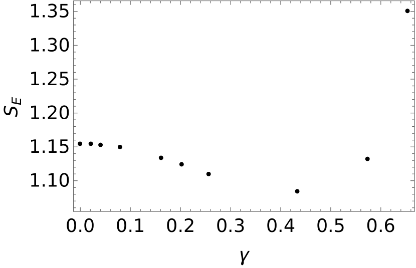
Figure 6: Net entanglement entropy for pair production in a pulse as in (36) for $T=0.08$, $z_{M}=1$ and $\lambda=12$.

V Conclusions

In the semiclassical approximation at weak coupling, the Schwinger pair creation by an electric pulse is captured by a periodic worldline instanton. The inverse period of the instanton can be identified with the Unruh temperature.

The pair production in an electric pulse at strong coupling in the gravity dual description is described by a worldsheet instanton. We have found the corresponding worldsheet in Minkowski signature in the weak field limit. In the strong field limit, we have obtained numerically the tunneling surface, thereby generalizing the holographic Schwinger pair production process in a constant electric field Semenoff and Zarembo (2011) to time-dependent electric pulses.

Remarkably, the gravity dual string worldsheet exhibits a falling wormhole that acts as a separatrix splitting the worldsheet into a causal and acausal part which is hidden behind the horizon. In the weak field limit and under the assumption that $\omega$ is sufficiently large, the causal part of the worldsheet does not generate any entanglement entropy to leading order at late times, and all of it results from the radiation in the acausal part.

This is not the case in the strong field limit, where the causal part of the worldsheet can be captured by the Euclidean surface. Indeed, the numerically generated Euclidean worldsheet results in a positive contribution to the entanglement entropy.

It would be interesting to derive the strong field expression for the contribution to the entanglement entropy from radiation. Moreover, in the weak field limit, it would be illuminating to work out the subleading contributions to the causal part of the entanglement entropy and see if it yields a net positive entanglement entropy at intermediate times.

Acknowledgments

This work was supported by the U.S. Department of Energy, Office of Science, Office of Nuclear Physics, Grants Nos. DE-FG88ER41450 and DE-SC0012704 (DK), and the U.S. Department of Energy, Office of Science, National Quantum Information Science Research Centers, Co-design Center for Quantum Advantage (C2QA) under Contract No.DE-SC0012704 (DK).

References

- Schwinger (1951) Julian S. Schwinger, “On gauge invariance and vacuum polarization,” Phys. Rev. 82, 664–679 (1951).
- Andersson et al. (1983) Bo Andersson, G. Gustafson, G. Ingelman, and T. Sjostrand, “Parton Fragmentation and String Dynamics,” Phys. Rept. 97, 31–145 (1983).
- Buskulic et al. (1995) D. Buskulic et al. (ALEPH), “Measurements of the charged particle multiplicity distribution in restricted rapidity intervals,” Z. Phys. C 69, 15–26 (1995).
- Jensen and Karch (2013) Kristan Jensen and Andreas Karch, “Holographic Dual of an Einstein-Podolsky-Rosen Pair has a Wormhole,” Phys. Rev. Lett. 111, 211602 (2013), arXiv:1307.1132 [hep-th] .
- Sonner (2013) Julian Sonner, “Holographic Schwinger Effect and the Geometry of Entanglement,” Phys. Rev. Lett. 111, 211603 (2013), arXiv:1307.6850 [hep-th] .
- Gorsky et al. (2002) A. S. Gorsky, K. A. Saraikin, and K. G. Selivanov, “Schwinger type processes via branes and their gravity duals,” Nucl. Phys. B 628, 270–294 (2002), arXiv:hep-th/0110178 .
- Xiao (2008) Bo-Wen Xiao, “On the exact solution of the accelerating string in AdS(5) space,” Phys. Lett. B 665, 173–177 (2008), arXiv:0804.1343 [hep-th] .
- Semenoff and Zarembo (2011) Gordon W. Semenoff and Konstantin Zarembo, “Holographic Schwinger Effect,” Phys. Rev. Lett. 107, 171601 (2011), arXiv:1109.2920 [hep-th] .
- Lewkowycz and Maldacena (2014) Aitor Lewkowycz and Juan Maldacena, “Exact results for the entanglement entropy and the energy radiated by a quark,” JHEP 05, 025 (2014), arXiv:1312.5682 [hep-th] .
- Chernicoff et al. (2013) Mariano Chernicoff, Alberto Güijosa, and Juan F. Pedraza, “Holographic EPR Pairs, Wormholes and Radiation,” JHEP 10, 211 (2013), arXiv:1308.3695 [hep-th] .
- Jensen et al. (2014) Kristan Jensen, Andreas Karch, and Brandon Robinson, “Holographic dual of a Hawking pair has a wormhole,” Phys. Rev. D 90, 064019 (2014), arXiv:1405.2065 [hep-th] .
- Hubeny and Semenoff (2014) Veronika E. Hubeny and Gordon W. Semenoff, “Holographic Accelerated Heavy Quark-Anti-Quark Pair,” (2014), arXiv:1410.1172 [hep-th] .
- Ghodrati (2015) Mahdis Ghodrati, “Schwinger Effect and Entanglement Entropy in Confining Geometries,” Phys. Rev. D 92, 065015 (2015), arXiv:1506.08557 [hep-th] .
- Semenoff (2018) Gordon W. Semenoff, “Lectures on the holographic duality of gauge fields and strings,” (2018), 10.1093/oso/9780198828150.003.0003, arXiv:1808.04074 [hep-th] .
- Yeh (2023) Chen-Pin Yeh, “Shock Waves in Holographic EPR pair,” (2023), arXiv:2310.00991 [hep-th] .
- Maldacena and Susskind (2013) Juan Maldacena and Leonard Susskind, “Cool horizons for entangled black holes,” Fortsch. Phys. 61, 781–811 (2013), arXiv:1306.0533 [hep-th] .
- Grieninger et al. (2023) Sebastian Grieninger, Dmitri E. Kharzeev, and Ismail Zahed, “Entanglement in a holographic Schwinger pair with confinement,” Phys. Rev. D 108, 086030 (2023), arXiv:2305.07121 [hep-th] .
- Hubeny and Semenoff (2015) Veronika E. Hubeny and Gordon W. Semenoff, “String worldsheet for accelerating quark,” JHEP 10, 071 (2015), arXiv:1410.1171 [hep-th] .
- Gelis et al. (2010) Francois Gelis, Edmond Iancu, Jamal Jalilian-Marian, and Raju Venugopalan, “The Color Glass Condensate,” Ann. Rev. Nucl. Part. Sci. 60, 463–489 (2010), arXiv:1002.0333 [hep-ph] .
- Kovchegov and Levin (2013) Yuri V. Kovchegov and Eugene Levin, Quantum Chromodynamics at High Energy, Vol. 33 (Oxford University Press, 2013).
- Bjorken (1992) James D Bjorken, “How black is a constituent quark??” Acta Physica Polonica B 23, 637 (1992).
- Florio and Kharzeev (2021) Adrien Florio and Dmitri E Kharzeev, “Gibbs entropy from entanglement in electric quenches,” Physical Review D 104, 056021 (2021).
- Casini et al. (2011) Horacio Casini, Marina Huerta, and Robert C. Myers, “Towards a derivation of holographic entanglement entropy,” JHEP 05, 036 (2011), arXiv:1102.0440 [hep-th] .
- Brezin and Itzykson (1970) E. Brezin and C. Itzykson, “Pair production in vacuum by an alternating field,” Phys. Rev. D 2, 1191–1199 (1970).
- Popov (1971) V. S. Popov, “Pair production in a variable external field (quasiclassical approximation),” Zh. Eksp. Teor. Fiz. 61, 1334–1351 (1971).
- Kim and Page (2002) Sang Pyo Kim and Don N. Page, “Schwinger pair production via instantons in a strong electric field,” Phys. Rev. D 65, 105002 (2002), arXiv:hep-th/0005078 .
- Dunne and Schubert (2005) Gerald V. Dunne and Christian Schubert, “Worldline instantons and pair production in inhomogeneous fields,” Phys. Rev. D 72, 105004 (2005), arXiv:hep-th/0507174 .
- Kharzeev and Tuchin (2005) Dmitri Kharzeev and Kirill Tuchin, “From color glass condensate to quark–gluon plasma through the event horizon,” Nuclear Physics A 753, 316–334 (2005).
- Gies and Klingmuller (2005) Holger Gies and Klaus Klingmuller, “Pair production in inhomogeneous fields,” Phys. Rev. D 72, 065001 (2005), arXiv:hep-ph/0505099 .
- Gies and Torgrimsson (2016) Holger Gies and Greger Torgrimsson, “Critical Schwinger pair production,” Phys. Rev. Lett. 116, 090406 (2016), arXiv:1507.07802 [hep-ph] .
- Gies and Torgrimsson (2017) Holger Gies and Greger Torgrimsson, “Critical Schwinger pair production II - universality in the deeply critical regime,” Phys. Rev. D 95, 016001 (2017), arXiv:1612.00635 [hep-th] .
- Mikhailov (2003) Andrei Mikhailov, “Nonlinear waves in AdS / CFT correspondence,” (2003), arXiv:hep-th/0305196 .
- Shuryak et al. (2007) Edward Shuryak, Sang-Jin Sin, and Ismail Zahed, “A Gravity dual of RHIC collisions,” J. Korean Phys. Soc. 50, 384–397 (2007), arXiv:hep-th/0511199 .
- Kim et al. (2008) Keun-Young Kim, Sang-Jin Sin, and Ismail Zahed, “Diffusion in an expanding plasma using AdS/CFT,” JHEP 04, 047 (2008), arXiv:0707.0601 [hep-th] .
- Grieninger and Zahed (2023) Sebastian Grieninger and Ismail Zahed, “Out-of-equilibrium photon production and electric conductivity in a holographic Bjorken expanding plasma,” Phys. Rev. D 107, 046017 (2023), arXiv:2211.10372 [hep-ph] .