Observed Trends in FRB Population and Bi-modality in the Luminosity Density Distribution

Abstract

We have considered both non-CHIME and CHIME FRBs in the present study. Our robust conclusion is that there are two categories of non-CHIME FRBs - high luminosity density and low luminosity density events, with majority of the repeaters falling in the latter category. In order to circumvent the non-availability of measured fluence and flux density of the CHIME FRBs, we have devised a novel dimensionless approach that utilizes the ratio of the estimated CHIME lower limits to the fluence as well as to the flux density to investigate the presence of trends and patterns in both non-CHIME as well as CHIME FRB population. We have introduced several physically meaningful dimensionless quantities, and one of the robust results is that the computed values of these are almost same for both CHIME and non-CHIME events. This universality is also seen in the distributions of the computed dimensionless quantities and the underlying trends. In the case of CHIME repeaters, distributions of few of the dimensionless quantities hint at the existence of two modes of repeating radio transients.

1 Introduction

The first reported fast radio burst (FRB) was discovered serendipitously from the Parkes telescope archival data by Lorimer et al. (2007) [1]. Since then numerous other FRBs have continued to be gleaned from different radio bands, ranging from 110 MHz to about 8 GHz, by a host of radio telescopes.

FRBs are luminous radio sources that are sporadic, distant, appearing from random directions and lasting for about a few milliseconds. From the observed large dispersion measures (DMs) associated, in general, with these radio transients, their extra-galactic origin is almost certain. While a majority of the FRB events are one-off affairs individually, several of the FRBs are repeaters including FRB 20121102A (the first ever repeater discovered [2]) located in a star-forming dwarf galaxy having a redshift $z=0.19$ ([3]-[5]). The all-sky FRB event rate has been estimated to be fairly large $\sim 10^{4}$ [6].

Active radio transients from two of the repeaters - FRB 20121102A and FRB 20180916B, appear to be bunched with observed inter-bunch gaps of $\sim$ 157 days and $\sim$ 16 days, respectively, random occurrences within a bunch notwithstanding. All the aforementioned points have been discussed comprehensively and thoroughly in many excellent reviews on the subject (e.g. [7]- [12]). Because of the milli-second nature of the FRB durations, there are roughly two broad classes of models that are pursued seriously - one associated directly with magnetars (e.g. [6], [13]-[20]) and the other, with the gravitational collapse of supra-massive spinning neutron stars ([21]-[23]).

After the discovery of a low luminosity Galactic radio burst (FRB 20200428A) along with an associated X-ray burst from a Soft Gamma Repeater (SGR) - the magnetar SGR 1935+2154 ([24]-[29]), the balance tilted somewhat in favour of the magnetar origin for at least a group of FRBs. However, the Five-hundred-meter Aperture Spherical Radio Telescope (FAST) has not seen any FRB-SGR connection so far, indicating that transient radio emission from magnetars during their soft gamma radiation phase is extremely rare ([30],[10]). Furthermore, searches for high energy counterparts of FRBs have also led to low values of stringent upper limits on the flux densities of high energy photons ([31]-[34]).

In spite of a large body of research papers that continue to explore the theoretical modeling of FRBs, the real physical nature of these perplexing objects is still an enigma and is an area of active investigation. Therefore, it is very crucial to search for patterns that emerge from the observed FRB data in order to reach closer to the physical nature of FRBs. Some general trends that have ensued are that repeaters tend to have a larger observed duration than the non-repeaters and that the spectral width of the former is narrower leading to a wide variation in their spectral index values ([35],[12]).

In this letter, by considering first the distribution of radio luminosity densities of non-CHIME FRBs, we present statistical evidence that suggests the existence of two categories of radio transients- a high luminosity density category and a lower one. The analysis assumed that most of the non-repeating FRBs have a spectral index value of 1.5 while the spectral index of various recurrences of radio transients from repeaters lie in a broad interval, ranging from -2 to 1.5.

Since only lower limits to the FRB fluence and flux density can be obtained from the CHIME catalog, we have introduced a new technique that makes use of the ratio of fluence to flux density for each FRB and have carried out an investigation to demonstrate the existence of similar statistical patterns for both CHIME as well as non-CHIME FRBs.

2 Basic Framework

For a radio transient source with a power law spectrum, the intrinsic luminosity density may be expressed,

$$L_{\nu}(t)=L_{0}(t)\ \nu^{-\alpha}\ ,$$ (1)

where $L_{0}(t)$, $\alpha$, $\nu$, and $t$ are the time-dependent source luminosity parameter, spectral index, frequency and time in the rest frame of the source, respectively.

In the case of a $\Lambda$CDM model, the observed flux density then is given by,

$$S_{\nu_{O}}(t_{O})=\frac{(1+z)L_{\nu_{O}(1+z)}(t)}{4\pi D^{2}_{L}(z)}=$$ (2)

$$=\frac{(1+z)^{1-\alpha}\nu^{-\alpha}_{O}L_{0}(t)}{4\pi D^{2}_{L}(z)}$$ (3)

where $z$, $\nu_{O}$, $t_{O}$ and $D_{L}(z)$ are the source cosmological redshift, observed frequency, cosmic time in the observer’s rest frame and the luminosity distance of the source, respectively, with,

$$D_{L}(z)=\frac{c}{H_{0}}\int_{0}^{z}\frac{dz^{\prime}}{\sqrt{\Omega_{\Lambda,0}+\Omega_{m,0}(1+z^{\prime})^{3}}}\ \ .$$ (4)

Throughout the paper, to evaluate the luminosity distance from eq(4), we have used the following values for the cosmological parameters: $H_{0}=73.04$ km/s/Mpc, $\Omega_{m,0}=0.28$ and $\Omega_{\Lambda,0}=0.72$.

The observed fluence is given by,

$$F_{\nu_{O}}=\int^{t_{O}+\Delta t_{O}}_{t_{O}}{S_{\nu_{O}}(t^{\prime})\ dt^{\prime}}\ \ ,$$ (5)

where $\Delta t_{O}=(1+z)\Delta t$ is the observed time duration of the source while $\Delta t$ is the intrinsic duration of the transient source in its rest frame.

The energy released by the source is given by,

$$E=\int^{\nu_{2}}_{\nu_{1}}{d\nu{\int^{t+\Delta t}_{t}{L_{\nu}(\tau)d\tau}}}$$ (6)

so that, after making use of eqs. (3) and  (5) in the above, we obtain,

$$E=4\pi D^{2}_{L}(z)(1+z)^{\alpha-2}F_{\nu_{O}}\ \nu^{\alpha}_{O}\bigg{[}\frac{\nu^{1-\alpha}_{1}-\nu^{1-\alpha}_{2}}{\alpha-1}\bigg{]}$$ (7)

In the literature, the redshifts of the repeating FRBs are estimated from the accurately measured redshifts of their host galaxies while the observed dispersion measures (DMs) are used to estimate the cosmological redshifts of the non-repeating FRBs. The local contributions like from the source Doppler shift or from gravitational redshifts to the overall redshift of a FRB are, in general, negligible. For instance, if a source has a speed $\sim 300$ km/s with respect to the cosmological rest frame, the corresponding Doppler shift is only $\sim 10^{-3}$.

As far as gravitational redshift is concerned, emissions from around a massive and near-spherical object of mass $M$ and size $R\geq 2GM/c^{2}$ would incur a gravitational redshift $z_{gr}$ when observed at $r_{obs}\gg R$,

$$z_{gr}(R)\cong\sqrt{\frac{1-\frac{2GM}{c^{2}r_{obs}}}{1-\frac{2GM}{c^{2}R}}}-1\approx\bigg{(}1-\frac{2GM}{c^{2}R}\bigg{)}^{-1/2}-1\ \ .$$ (8)

So, according to eq. (8), FRB radiation climbing out of the gravitational potential of a galaxy of mass $\sim 10^{12}\ M_{\odot}$ and radial size $\sim 15$ kpc, would undergo a gravitational redshift $z_{gr}\sim 10^{-6}$, which is negligible.

However, in the context of magnetar-centric FRB models, if a radio transient is assumed to originate from a location close to the surface of a magnetar of mass $\sim 2\ M_{\odot}$ and radius $\sim 12$ km, the corresponding gravitational redshift is $\sim 0.4$, which cannot be ignored. On the other hand, if the emission takes place at distances closer to the light cylinder $R_{lc}$ of the magnetar,

$$R_{lc}=\frac{cP}{2\pi}\approx 50\ \bigg{(}\frac{P}{10^{-3}\ s}\bigg{)}\ \mbox{km}\ \ ,$$ (9)

the gravitational redshift caused by even a milli-second magnetar’s gravity is not very appreciable, since from eqs. (8) and  (9), $z_{gr}(R_{lc})\cong 0.066$ if the magnetor’s mass and radius are $\sim 2\ M_{\odot}$ and $\sim 12$ km, respectively. Therefore, one may consider only the cosmological redshift $z$ in the analysis, as it is the dominant component.

In terms of the observed quantities, the source luminosity density at the rest frequency of 300 MHz can be obtained from eq. (2),

$$L_{300}\equiv 4\pi D^{2}_{L}(z)(1+z)^{\alpha-1}S_{\nu_{O}}\bigg{(}\frac{\nu_{O}}{300\ \mbox{MHz}}\bigg{)}^{\alpha}$$ (10)

In an analogous manner, the expression for the luminosity density at any specified frequency can be expressed.

The brightness temperatures of FRBs are estimated to be very high, $(T_{b})_{FRB}\gtrsim 10^{36}\ {}^{\circ}$K ([36],[37]). From special relativity and causality arguments, it follows that the FRB emission region has a size $l_{em}$ satisfying the constraint $l_{em}\lesssim c\Delta t$ so that the brightness temperature of the source in its rest frame is given by ([38],[12]),

$$(T_{b})_{FRB}\cong\bigg{(}\frac{c^{2}}{2\pi k_{B}\nu^{2}_{O}}\bigg{)}S_{\nu_{O}}(1+z)\bigg{(}\frac{D_{A}(z)}{l_{em}}\bigg{)}^{2}$$ (11)

$$\gtrsim T_{b}\cong\bigg{(}\frac{c^{2}}{2\pi k_{B}\nu^{2}_{O}}\bigg{)}S_{\nu_{O}}(1+z)\bigg{(}\frac{D_{A}(z)}{c\Delta t}\bigg{)}^{2}$$ (12)

$$=\frac{S_{\nu_{O}}D^{2}_{L}(z)(1+z)}{k_{B}\bigg{(}\Delta t_{O}\ \nu_{O}(1+z)\bigg{)}^{2}}\ \ ,$$ (13)

where $D_{A}(z)=D_{L}(z)/(1+z)^{2}$ is the angular diameter distance.

The above considerations can also be used to estimate a lower bound to the energy density of the radio photons within the emitting region,

$$u_{FRB}\cong\frac{E}{l^{3}_{em}}\gtrsim u\cong\frac{E}{(c\Delta t)^{3}}$$ (14)

The energy density $u_{FRB}$ is very likely to be associated significantly with the ambient magnetic field.

It is useful to define dimensionless quantities that make use of various measured physical quantities related to the FRBs in order that we may compare the obtained outcomes for both non-CHIME as well as CHIME FRBs. Since the CHIME catalog only provides lower bounds to the fluence and flux density of individual radio transients, we have introduced a new technique that involves taking the ratio of fluence to flux density and vice versa, so that the dimensionless quantities defined below can be computed for CHIME FRBs too (except for the quantity $X5$, which is a dimensionless characterization of the energy density $u$).

$$X1\equiv\frac{E\ \ L_{300}}{(F^{2}_{\nu_{O}}+S^{2}_{\nu_{O}}\Delta t^{2}_{O})\nu_{O}^{2}(\frac{DM}{n_{e}})^{4}}$$ (15)

$$X2\equiv\frac{E\ \ L_{300}}{(F^{2}_{\nu_{O}}+S^{2}_{\nu_{O}}\Delta t^{2}_{O})(\frac{DM}{n_{e}})^{2}c^{2}}$$ (16)

$$X3\equiv\frac{L_{300}}{\sqrt{(F^{2}_{\nu_{O}}+S^{2}_{\nu_{O}}\Delta t^{2}_{O})}\ \nu_{O}(\frac{DM}{n_{e}})^{2}}$$ (17)

$$X4\equiv\frac{u}{L_{300}}.\big{(}\frac{DM}{n_{e}}\big{)}^{3}\ ;\ X5\equiv\frac{u\ \ c^{3}}{h\nu^{4}_{O}}\ ;\ X6\equiv\frac{k_{B}\ T_{b}}{E}$$ (18)

In the above expressions, $n_{e}$ is a fixed fiducial number density of electrons used in order to obtain a ‘length’ dimension from the DM. In this paper, we have set $n_{e}=0.03\ \mbox{cm}^{-3}$, the value of the Galactic disc electron number density.

3 Data

The non-CHIME FRB data analyzed in the present work is obtained from the Transient Name Server (TNS) website $https://www.wis-tns.org/$. A majority of these transient events were detected using telescopes like the Australian Square Kilometre Array Pathfinder (ASKAP), Parkes, Arecibo, etc. While the Canadian Hydrogen Intensity Mapping Experiment (CHIME) data is taken from the CHIME/FRB first catalog paper from the CHIME data website $https://www.chime-frb.ca/catalog$ [39].

The redshift information for non-CHIME one-off FRBs has been taken from FRBSTATS [40] and the corresponding data for non-repeaters (NRs) in the CHIME catalog from Tang et. al. [41]. We have also used the individual sub-burst data of FRB 20121102  ([2]-[5], [42]), and each of these sub-bursts have been treated as distinct bursts in our study, and have been classified as repeaters (REPs). We have adopted this classification for every repeater (e.g. sub-bursts of FRB 180916.J0158+65 [43]).

4 Analysis and Results

Spectral index for NRs is taken to be 1.5 throughout (this is found to be true for 23 ASKAP FRBs [44]), except in the cases of FRB 20070724A and FRB 20110523A for which the spectral indices are taken to be 4 and 7.8, respectively ([1],[45]). The spectral indices for REPs vary over a wide range, presumably because of their narrow spectral width [35,12]. For the calculations of energy as well as luminosity density (eqs. (7) and  (10)) and subsequent analysis, we have considered five independent trials in each of which a set of values of $\alpha\in$ $\{-2,-1.5,-1.3,-0.5,1.3,1.5\}$ are randomly chosen, using a uniform probability distribution, and assigned to the REPs. Thereafter, we have also considered another trial and in this sixth trial, all the REPs are assigned $\alpha=1.5$. The same procedure has been carried out for each of the recurrences of a CHIME repeater too. (For the constraints on the values of $\alpha$ see ([46]-[49])).

4.1 Non-CHIME

The distributions of FRB luminosity density, energy, energy density as well as the ratio of luminosity density to the energy have been studied in a comprehensive manner. Figures  1 to  6 describe the trends observed for the non-CHIME FRBs. Whenever necessary, the median values of the plotted quantities have been specified in the figures, separately for REPs and NRs. The luminosity density could be calculated for 194 FRB events based on the available flux density and the estimated redshift data.

The histograms of luminosity density at 300 MHz show bimodal distributions for all five trials of randomly assigned spectral indices to the REPs as well as for the sixth trial. For one such trial corresponding to the random assignment of spectral indices, the histogram is shown in fig. 1a. The number distribution $n(L_{300})$ exhibits a minimum at $L_{300}\cong 4\times 10^{33}$ erg/s/Hz. This is also verified in a bin-width independent analysis by considering the slope of,

$$N(\leq L_{300})\equiv\int^{L_{300}}_{0}{n(L)dL}$$ (19)

as a function of the luminosity density at 300 MHz. It is expected that if $n(L_{300})$ has a minimum, the slope will change from being positive to $0$ (near the location of the minimum) and then positive again. Indeed, as can be seen from fig. 1b, this slope vanishes around $\cong 4\times 10^{33}$ erg/s/Hz, thus confirming the inference that was based on fig. 1a.

The minimum occurs at $\cong 4\times 10^{33}$ erg/s/Hz for all the five trials that use random assignment of $\alpha$ values. For the sixth trial (i.e., $\alpha=1.5$ case), the minimum is located at $\cong 5\times 10^{33}$ erg/s/Hz. When an identical exercise was carried out for the luminosity density at 1 GHz case, the minimum in the distribution was found to be slightly lower, at $\cong 10^{33}$ erg/s/Hz.

Hence, the individual FRB events may be classified into two categories - high L, those with $L_{300}>4\times 10^{33}$ erg/s/Hz and a remaining weaker lot, low L, $L_{300}\lesssim 4\times 10^{33}$ erg/s/Hz. To check for the robustness of this classification, a Kolmogorov-Smirnov (K-S) test was performed for the non-CHIME data by considering two of the independent trials pertaining to the random assignment of $\alpha$ values to the repeating events, and asking whether both of them were realizations of a given distribution.

For 194 distinct FRB events, the K-S Statistic is 0.0773196 corresponding to the p-value 0.137894. Therefore, the null hypothesis that both of the trials come from the same parent distribution is not rejected at the 5 percent level.

Fig. 2 displays the histograms of $L_{300}$ distributions, distinguishing the FRB events belonging to REPs (represented by lilac colour) from that of the one-off FRBs (in light blue), for all the six independent trials. From the median values and the spread, in all six trials, it is evident that REPs on average fall in the low L category. The histograms of energy $E$ corresponding to the six trials show minima that vary appreciably with individual trials, and hence, the evidence for bi-modality is not very strong.

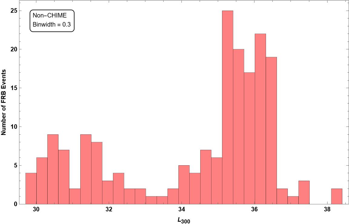
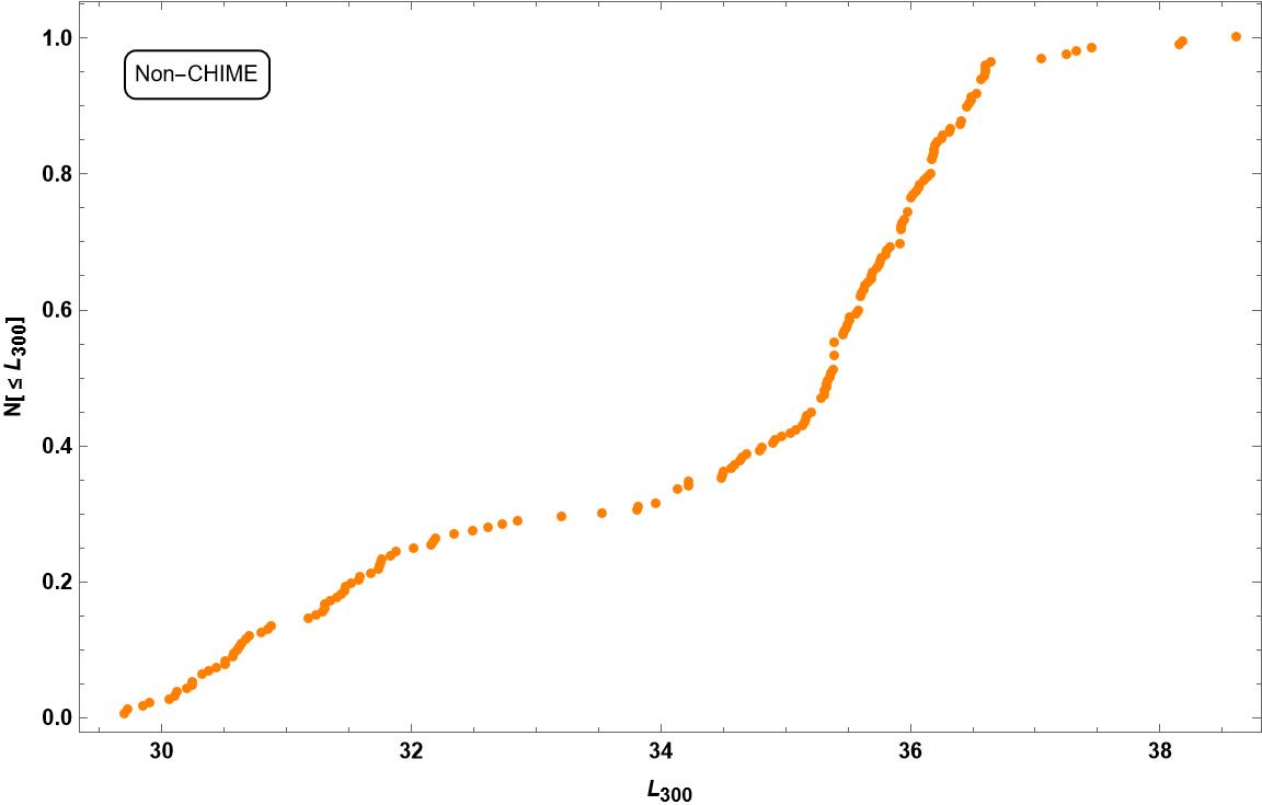
Figure 1: (a) A histogram for $L_{300}$ shows a bi-modality with a minimum at $L_{300}\cong 3.98\times 10^{33}$ erg/sec/Hz. (b) A bin-width independent way of arriving at the same conclusion is seen from the observed $N(\leq L_{300})$ versus $\log_{10}{(L_{300})}$ in which the slope is close to $\cong 0$ around $L_{300}\cong 3.98\times 10^{33}$ erg/sec/Hz.

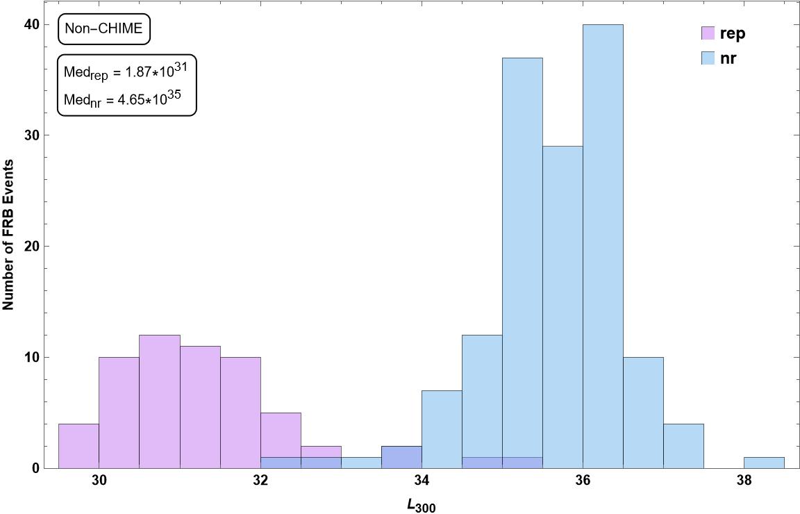
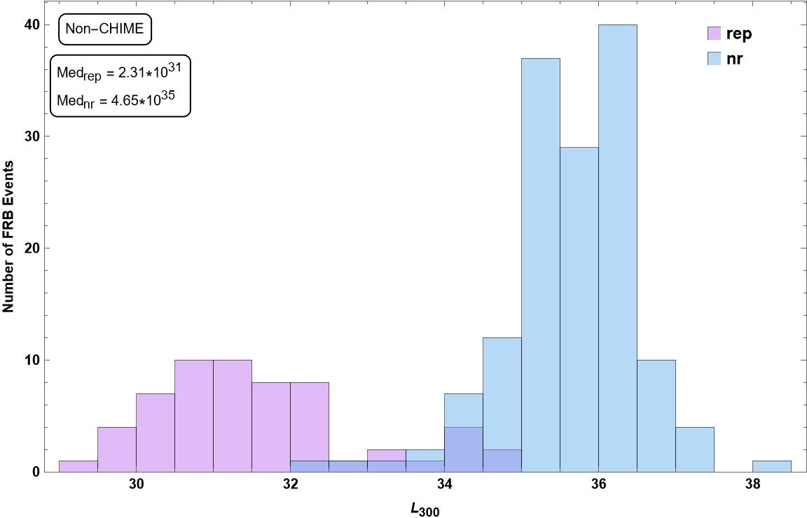
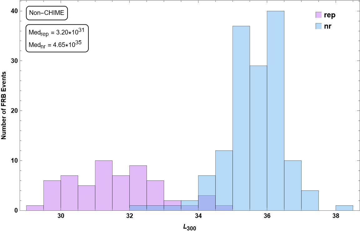
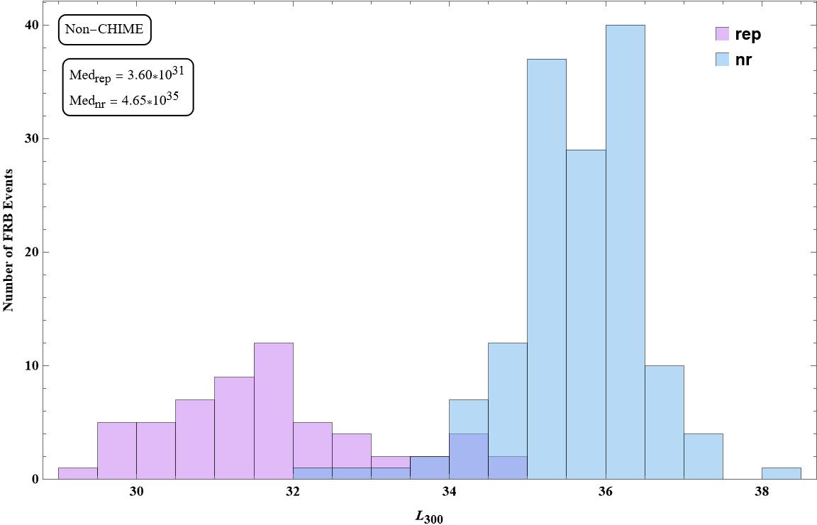
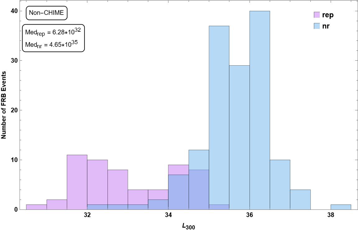
Figure 2: Histograms of $L_{300}$ of repeaters and non-repeaters. The first five figures correspond to five different sets in each of which the repeaters are assigned six randomly generated values of spectral index. The last histogram is for the case when all the repeaters are assigned $\alpha$=1.5.

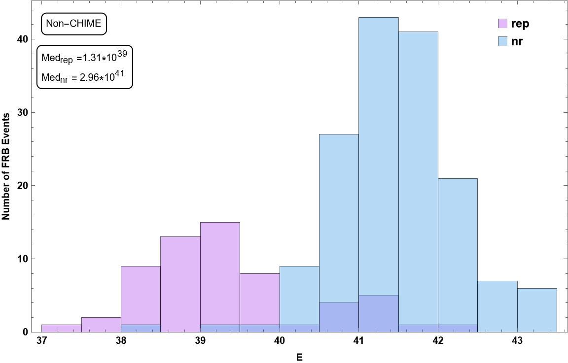
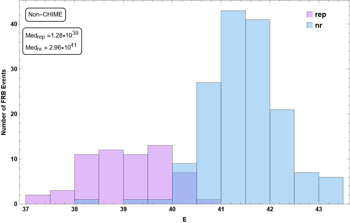
Figure 3: (a) A histogram of energy $E$ with repeaters assigned randomly a set of spectral indices. (b) A histogram of $E$ when $\alpha$ is set to be 1.5 for all the repeaters.

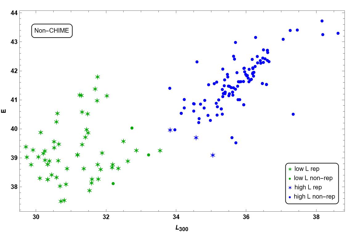
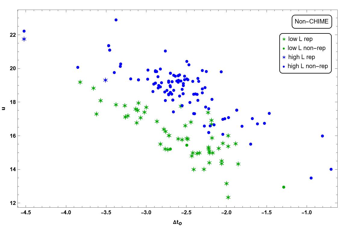
Figure 4: (a) A scatter plot of $E$ versus $L_{300}$ shows that they are statistically correlated with each other. (b) The energy density $u$ against observed duration $\Delta t_{O}$ shows segregation between the repeaters and the non-repeaters.

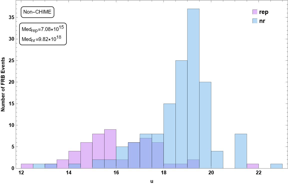
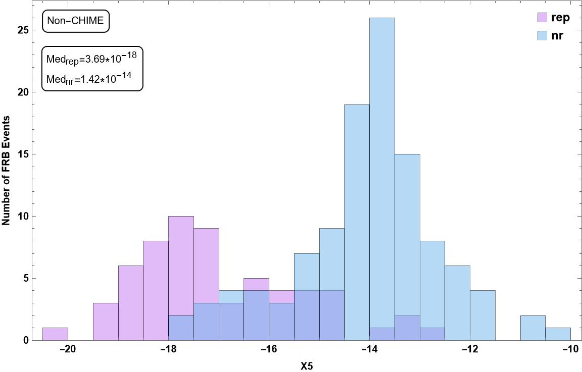
Figure 5: (a) A histogram of the energy density $u$ shows that the repeaters tend to have lower values of $u$ in comparison with that of the one-off FRBs. (b) A histogram of the dimensionless $X5$ also shows an appreciable segregation of repeaters from the one-off FRBs.

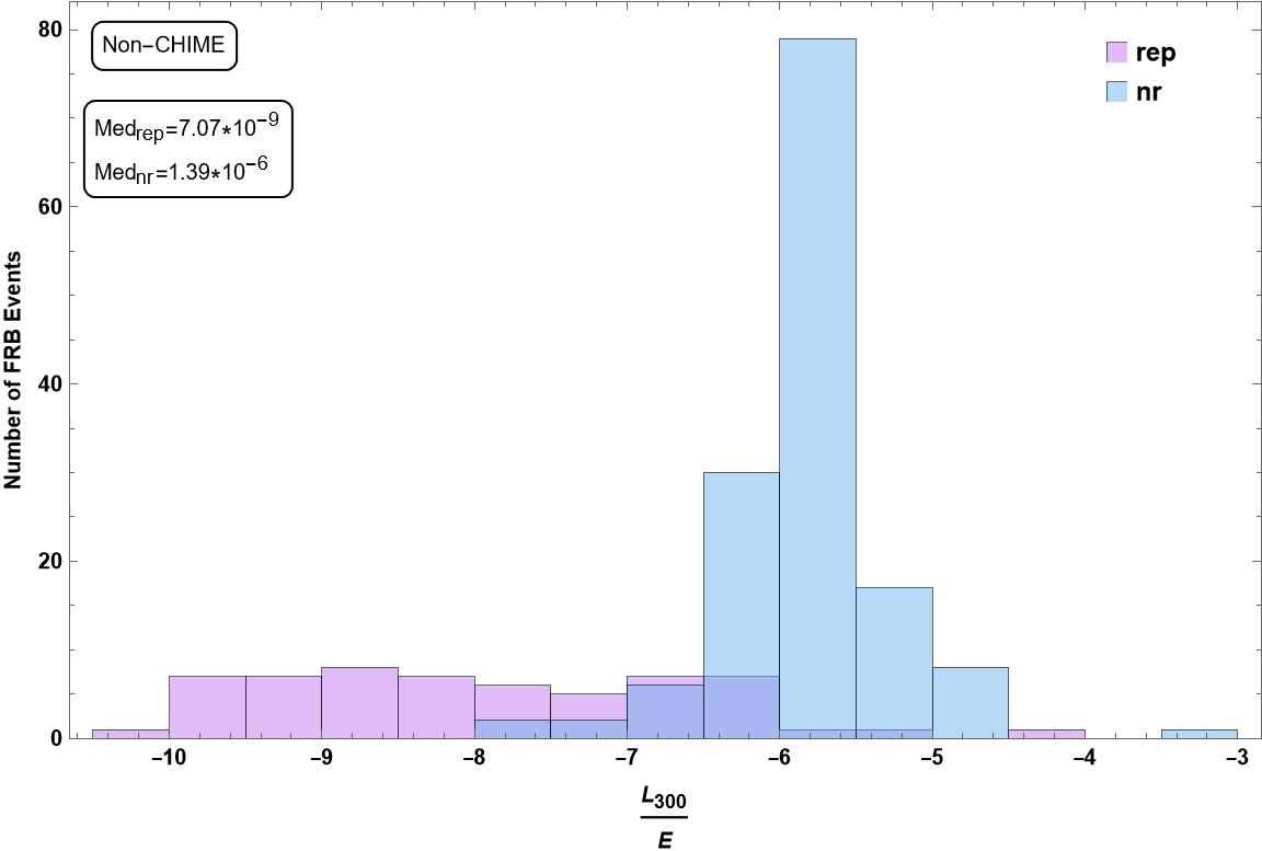
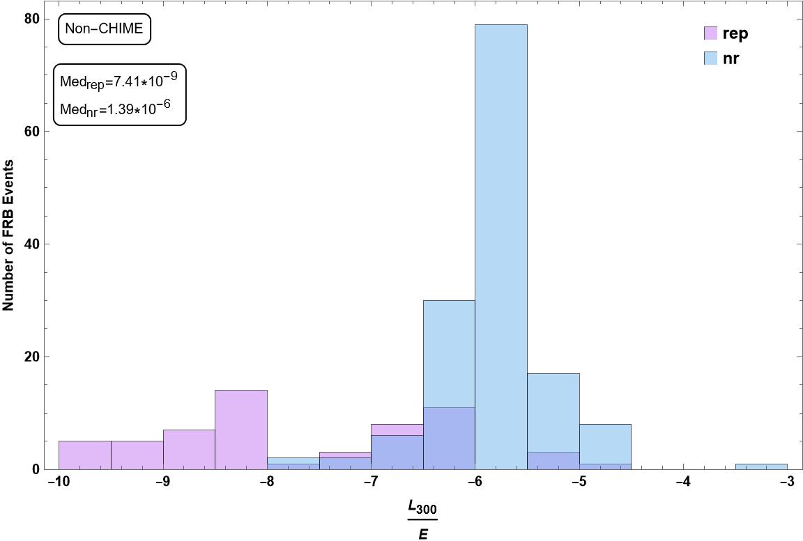
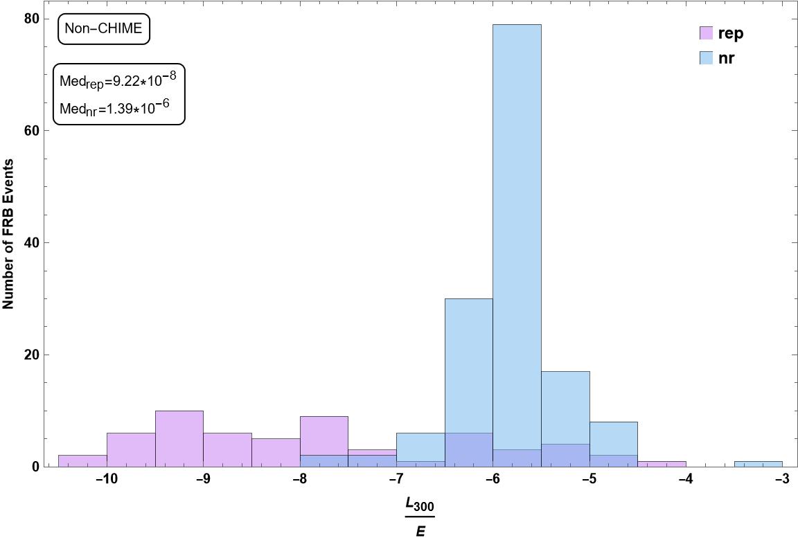
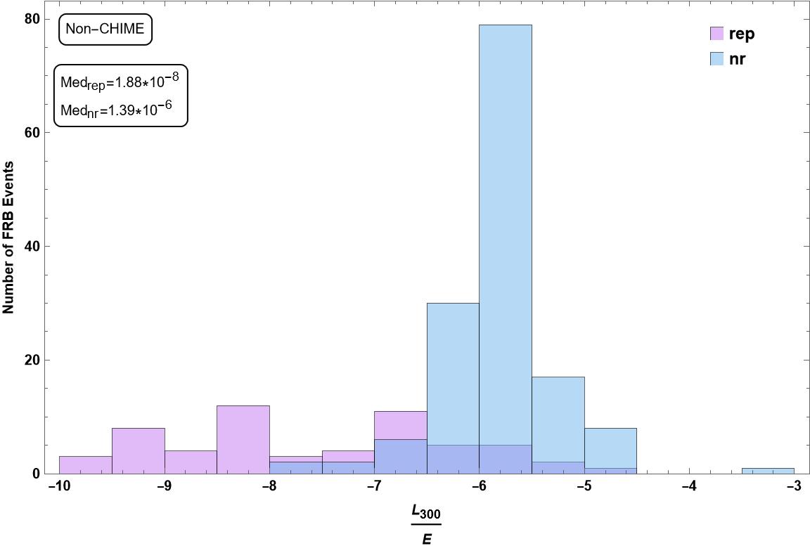
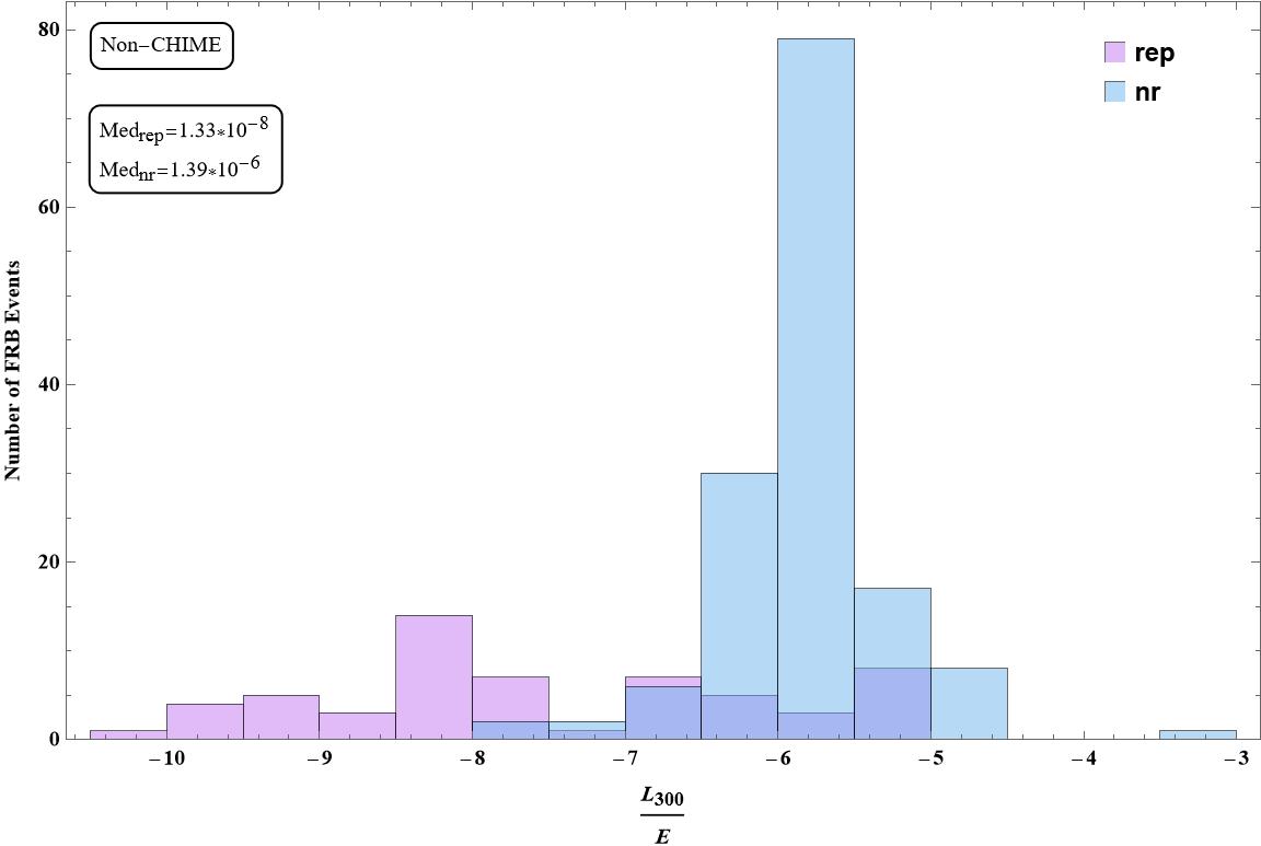
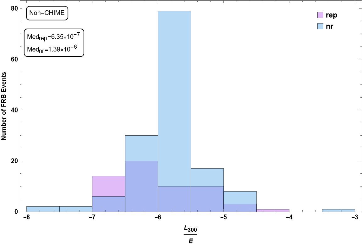
Figure 6: Histograms of the ratio of Luminosity density at 300 MHz to Energy for non-CHIME FRBs show bimodal behavior when repeaters are assigned six randomly generated values of the spectral index. The last figure corresponds to $\alpha$=1.5 assigned to all the repeaters.

Fig. 3a and Fig. 3b show the distributions of $E$ for (a) one of the trials pertaining to random assignment of $\alpha$ values and for (b) the sixth trial i.e., $\alpha=1.5$ to the REPs, respectively. From the median values of $E$ as well as the spread, one may infer that REPs tend to have lower values of $E$ compared to those of the NRs. The scatter plot is given in fig. 4a confirms this inference and points to the positive statistical correlation between luminosity density and energy of FRBs.

On the other hand, fig. 4b shows that for a given observed duration $\Delta t_{O}$, a non-repeater tends to be associated with somewhat greater lower limit to the energy density (i.e.,$u$). Since $u\approx E/(c\Delta t)^{3}$ the negative correlation seen in this figure between $u$ and $\Delta t_{O}$ is expected. From the histograms of figures. 5a and  5b (and the corresponding median values), it is quite clear that NRs tend to have larger values of $u$, which is consistent with the corresponding dimensionless $X5$ values.

The histograms presented in fig. 6 show that, for all the five trials, distributions of the ratio of $L_{300}$ to the energy $E$ as well as the corresponding median values point to REPs tending to have lower values of this dimensionless quantity compared to that of the NRs. However, for the sixth trial (i.e., $\alpha=1.5$ for all the REPs), the difference is very marginal. The interesting point is that since $L_{300}/E$ involves the ratio $S_{\nu_{O}}/F_{\nu_{O}}$, this analysis can be carried over to the CHIME FRBs as well.

4.2 CHIME

Given that a large number of the FRBs detected by CHIME are from off the center of the latter’s beam pattern, one can only set lower limits to the FRB’s actual flux density and fluence. However, for a CHIME FRB, it is reasonable to assume that the ratio of its measured flux density to fluence is close to the ratio had the FRB been detected in the direction coinciding with the beam center of the telescope. So, in order to compare the results we have obtained in the case of non-CHIME FRBs with the CHIME ones, we have introduced a new technique whereby we use the dimensionless quantities $L_{300}/E$, $X1$, $X2$, $X3$, $X4$ and $X6$ that involve the ratio $S_{\nu_{O}}/F_{\nu_{O}}$ (or its reciprocal) in our analysis for both these data sets.

The other advantage of this technique is that the numerical values of each of these dimensionless quantities lie in the same ranges for both CHIME and non-CHIME FRBs and hence, can be meaningfully compared. For instance, the histograms of fig. 7 demonstrate that distributions of $L_{300}/E$ and the corresponding median values of CHIME FRBs show the same trends as in the case of non-CHIME, entailing an internal consistency of our new method.

From fig. 8 to fig. 12, the distributions of the dimensionless quantities have been shown for both non-CHIME (left-hand panel) and CHIME FRBs (right-hand panel) for the purpose of comparisons. There is an overall agreement in the trends exhibited by the FRBs belonging to the two distinct data sets. Figs. 13a and  13b, although not dimensionless but involves the ratio $F_{\nu_{O}}/S_{\nu_{O}}$, show that the ratio of the lower limit to the energy density to the luminosity density tends to be larger for REPs in comparison to that of the NRs for non-CHIME FRBs and marginally larger for the CHIME ones. The histogram of $k_{B}T_{b}/E$ for the CHIME FRBs fig. 12b suggests that the NRs tend to have higher brightness temperatures than their repeating counterparts, although this trend is marginal for the non-CHIME FRBs fig. 12a.

Using both supervised [38] and unsupervised [50] machine learning methods, a recent study aimed to look for potential repeating FRBs among NRs in the CHIME first catalog. According to their findings, few of the earlier classified NRs are predicted to be potential REPs suggesting a search for recurring radio transients for these FRBs. The authors classify those potential REPs as strong which have been identified in both of the papers ([38],[50]). In the scatter plots of our present study, we represent the strong REP candidates with magenta asterisk, while those identified via an unsupervised (supervised) machine learning as type I (type II) REPs with blue (red) asterisk. In our analysis, from figs. 8b to  11b, it is very interesting to note that the majority of these potential REPs indeed follow the patterns that are common to the standard REPs.

Figs. 14a and  14b are for the CHIME bursts alone corresponding to a trial involving random assignment of $\alpha$ values to the REPs. The distributions of $X2$ and $X3$ as well as their median values reflect the tendency of NRs to have higher values than those of the REPs. Marginal bi-modalities are seen in the distributions of REPs entailing a hint of two distinct modes of radio-emission from the REPs. It may be pointed out, these trends survive even for the sixth trial (i.e. $\alpha=1.5$ for all the REPs). More future detections of REPs are required to strengthen this surmise.

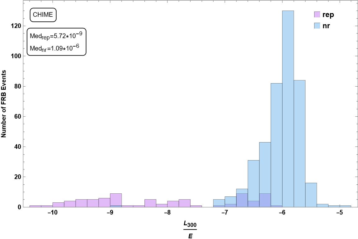
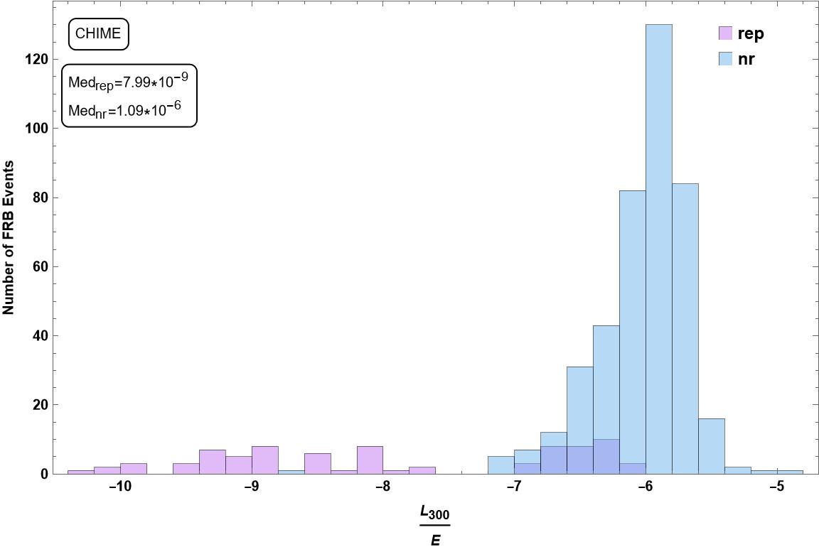
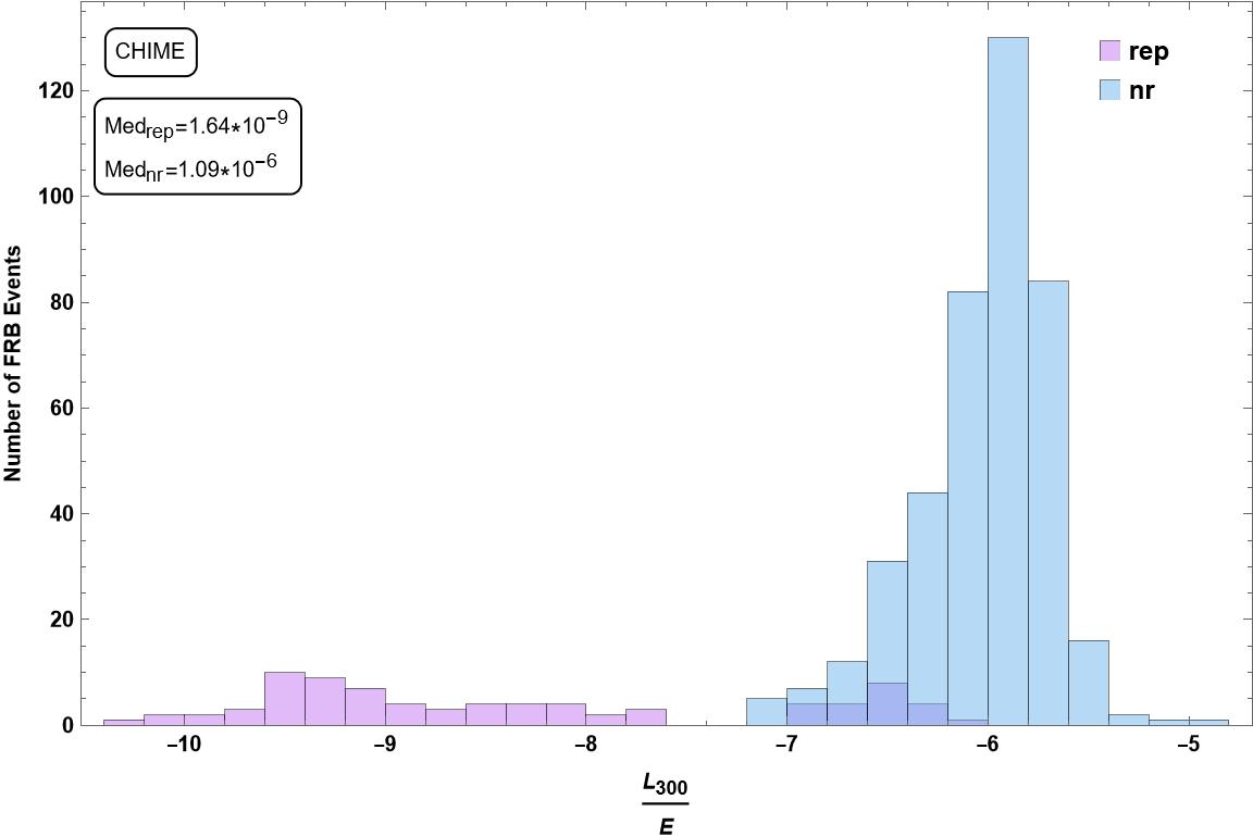
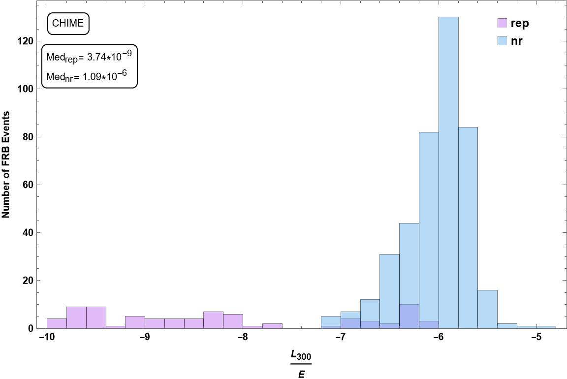
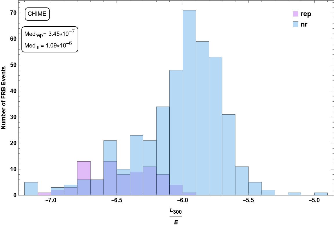
Figure 7: For CHIME FRBs, histograms of $L_{300}/E$ show similar bimodality when repeaters are given six randomly generated values of the spectral index. The last histogram corresponds to $\alpha$=1.5 being set for all the repeaters.

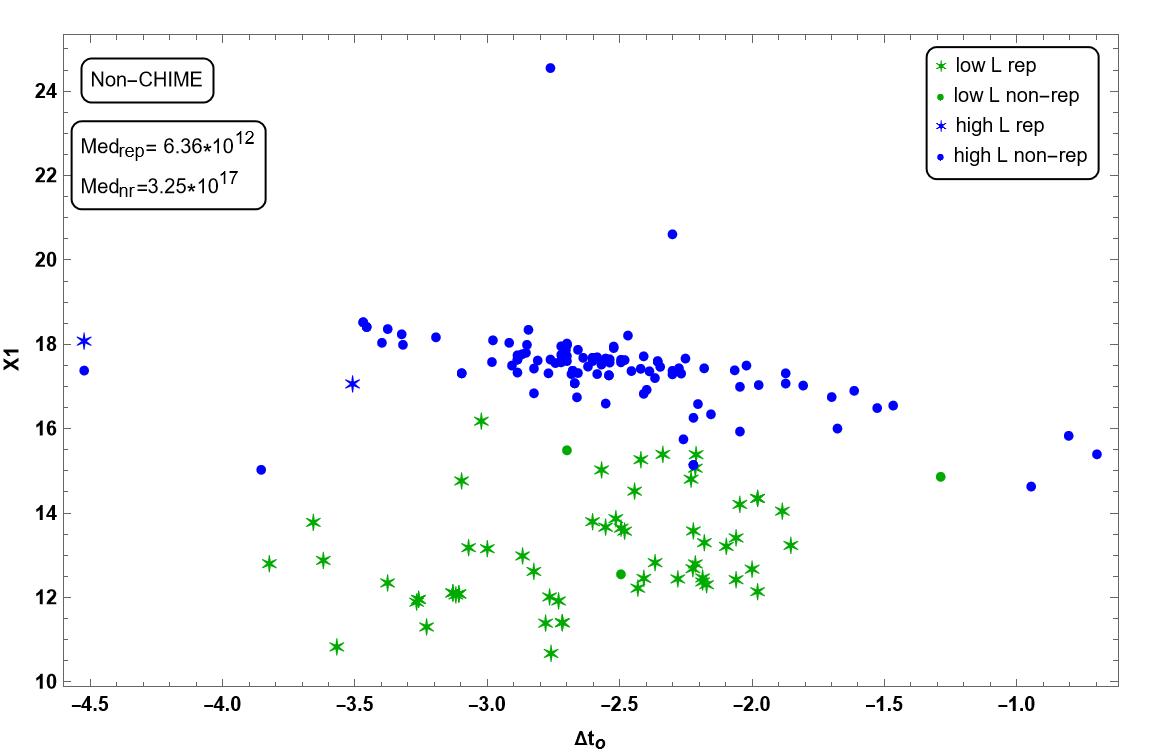
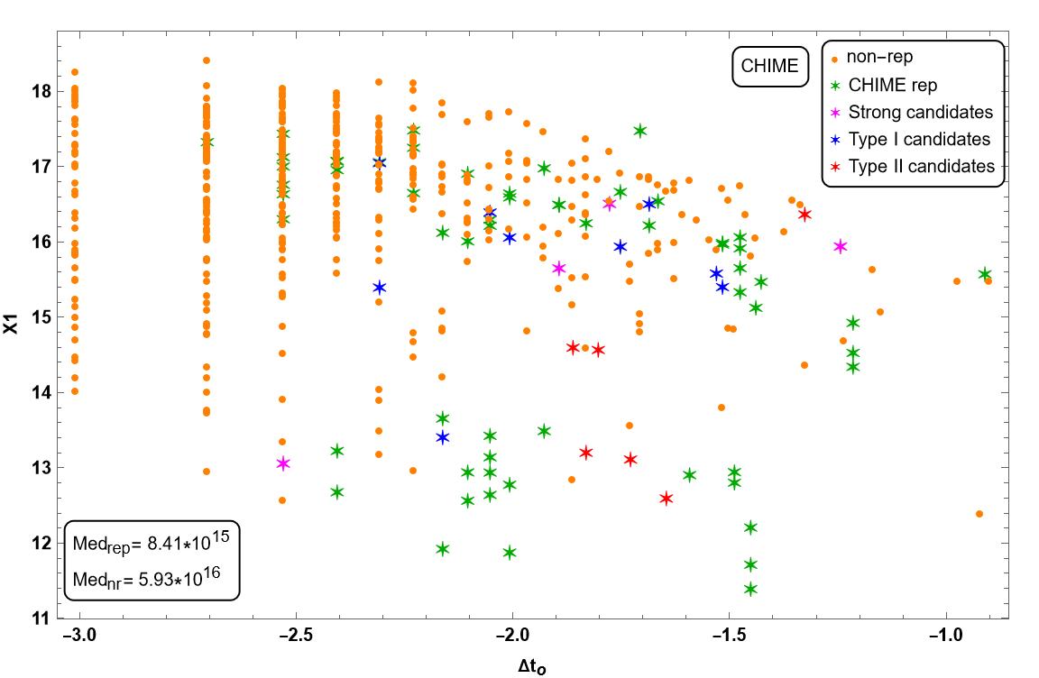
Figure 8: Scatter diagrams of $X1$ against the observed FRB duration for (a) non-CHIME and (b) CHIME. For both, repeaters tend to have lower values of $X1$.

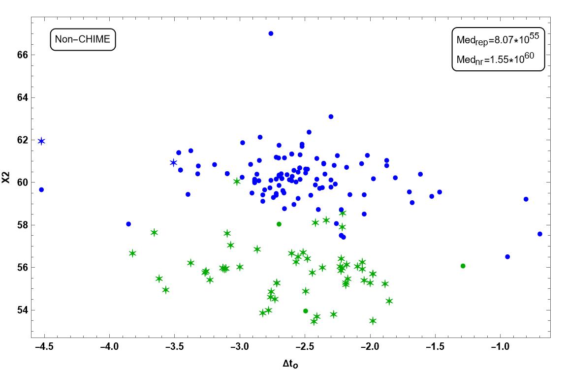
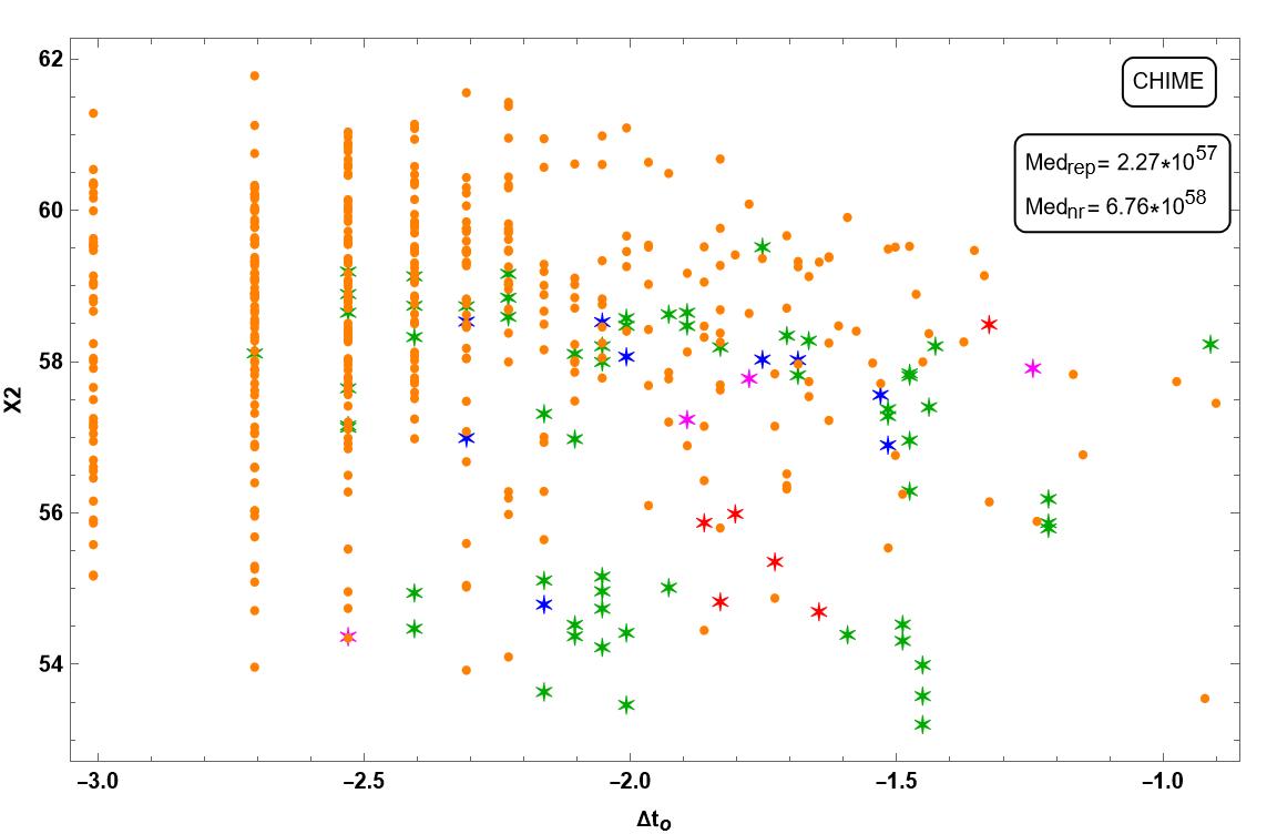
Figure 9: Scatter plots of $X2$ versus $\Delta t_{O}$ for (a) non-CHIME and (b) CHIME both show similar behavior with repeaters tending to have marginally smaller values of $X2$.

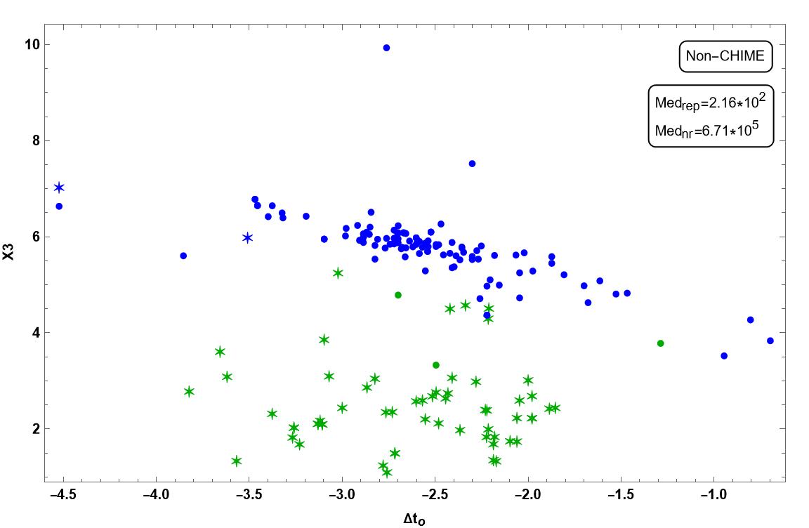
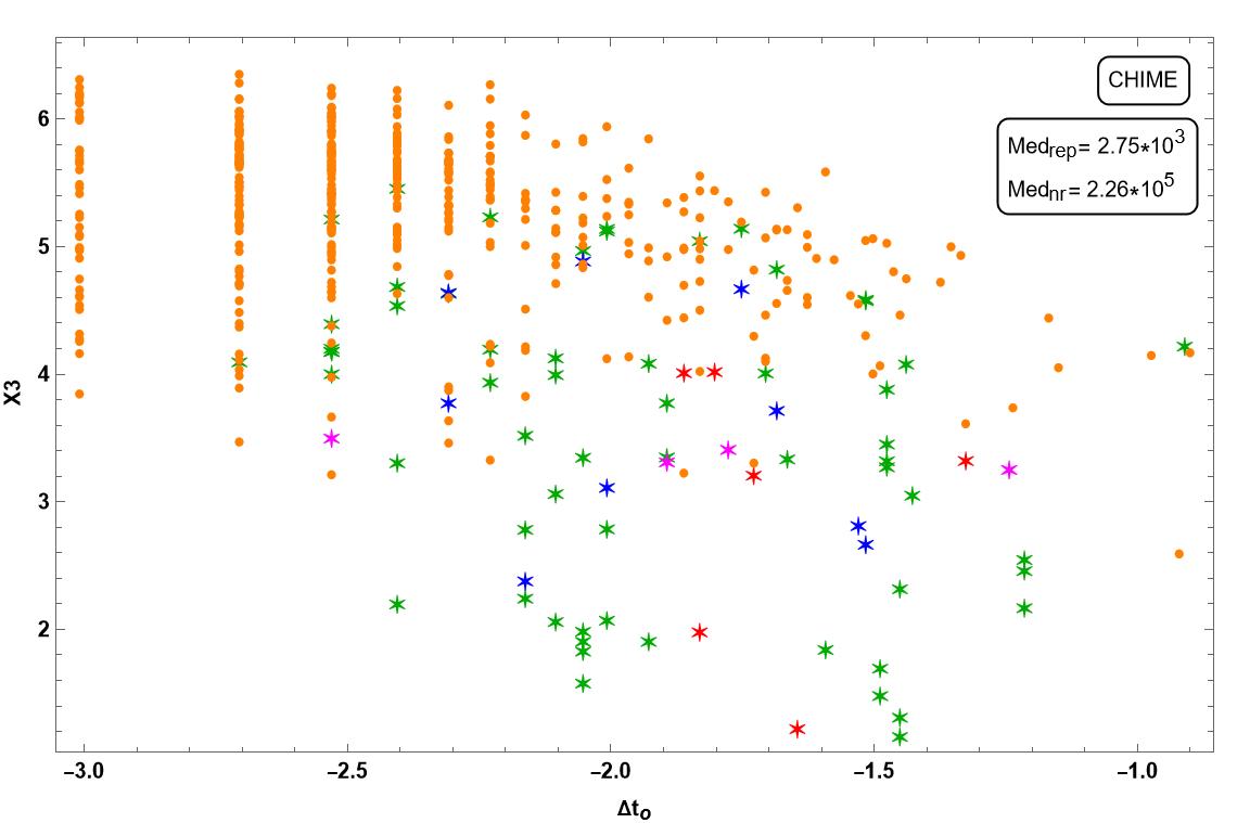
Figure 10: Scatter diagrams of $X3$ against $\Delta t_{O}$ for (a) non-CHIME and (b) CHIME both show similar trends, in that, repeaters tend to have lower values of $X3$.

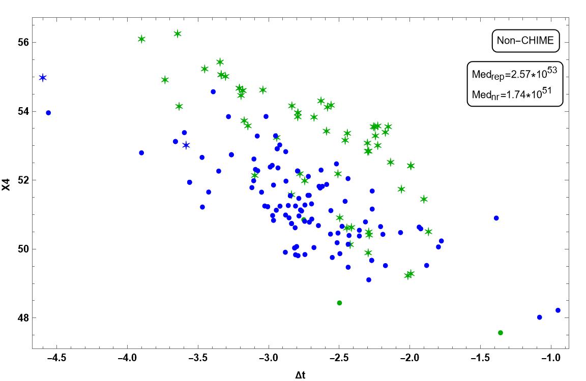
Figure 11: The dimensionless quantity $X4$ when plotted versus intrinsic duration $\Delta t$ show for (a) non-CHIME as well as (b) CHIME that $X4$ for the repeaters tend to lie to the right of those for the non-repeaters.

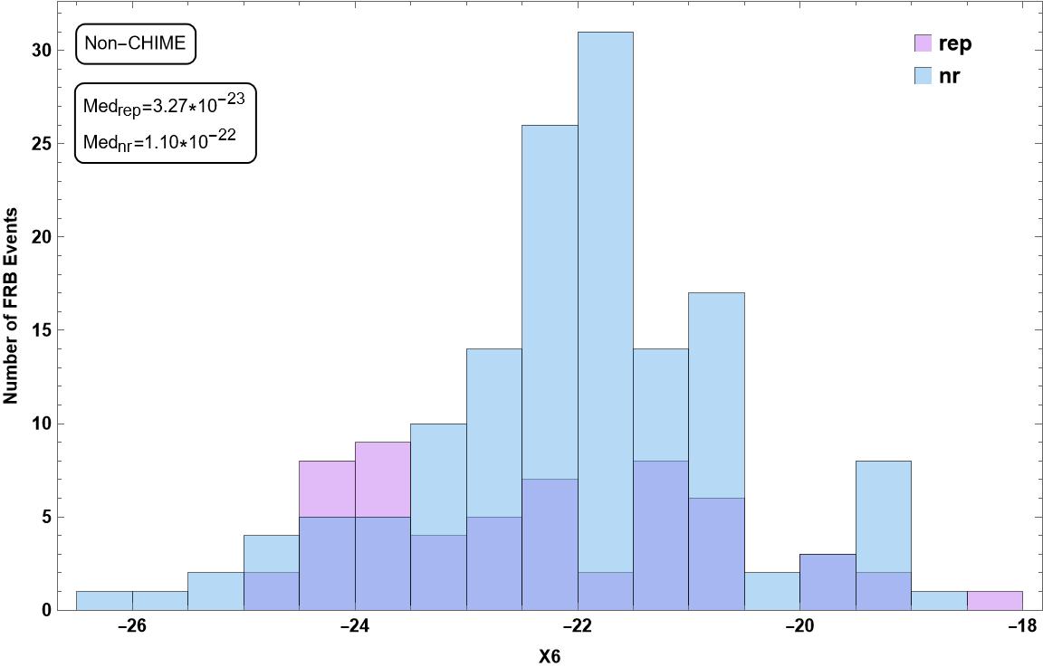
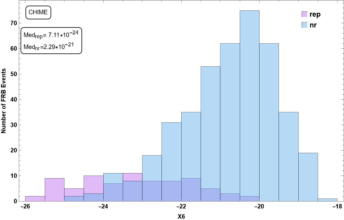
Figure 12: The CHIME histogram of the ratio $X6\equiv k_{B}\ T_{b}/E$ in (b) shows considerable separation in the peaks for REPs and NRs. In the case of (a) non-CHIME FRBs, the difference is marginal.

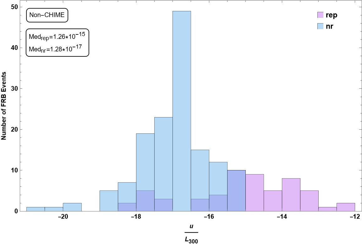
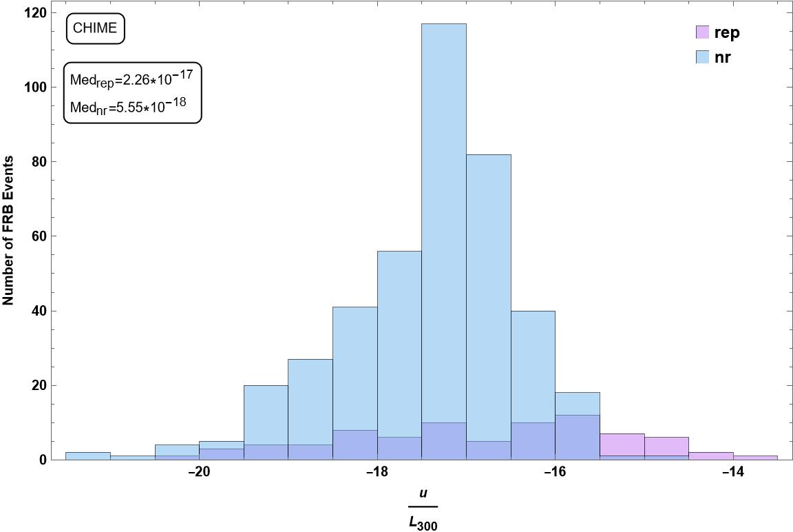
Figure 13: (a) A histogram of the energy density $u/L_{300}$ for non-CHIME shows that the repeaters tend to have higher values in comparison with that of the one-off FRBs. (b) A histogram of the dimensionless $X5$ shows the marginal segregation of repeaters and one-off FRBs and their distribution with repeaters tending to have lower values.

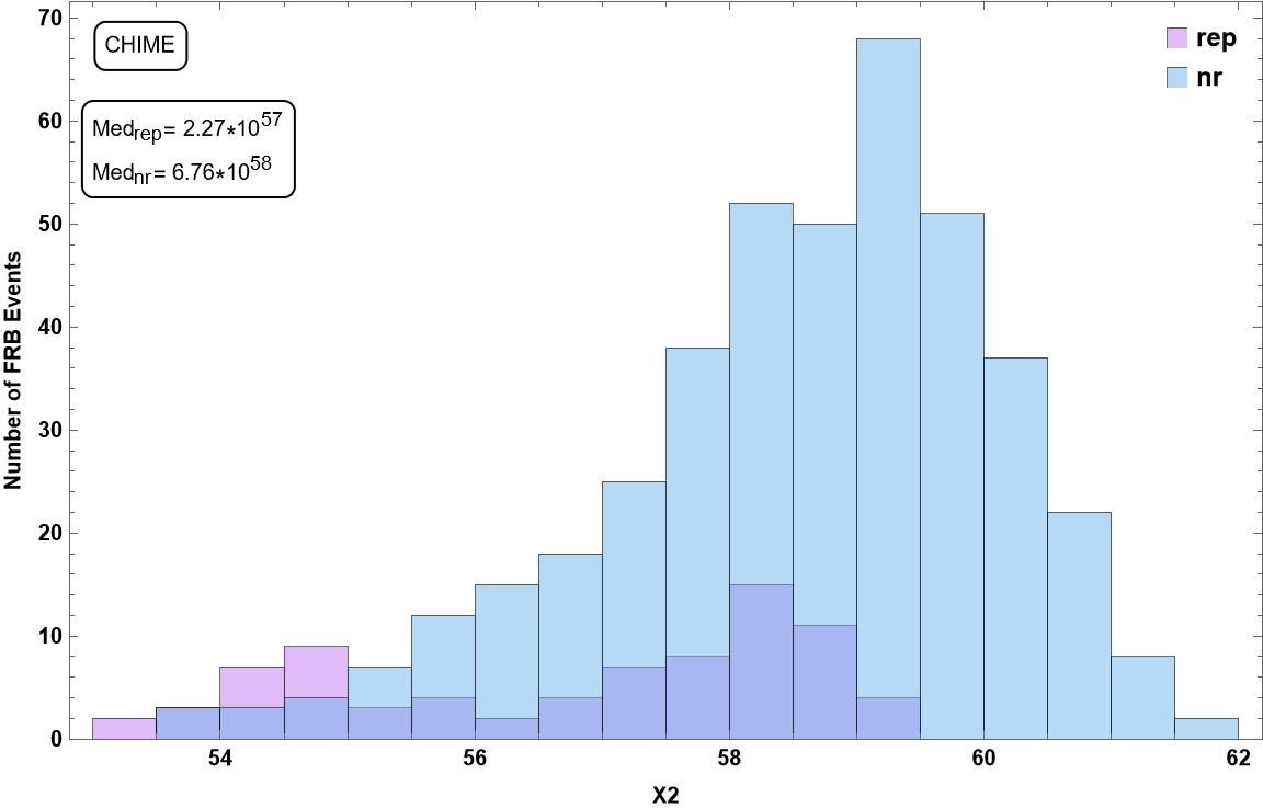
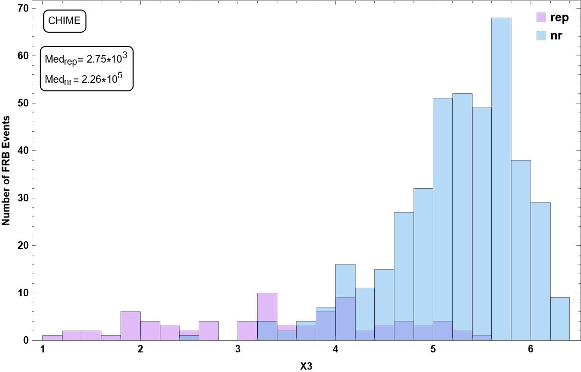
Figure 14: (a) The histograms for (a) $X2$ and (b) $X3$, for CHIME FRBs show segregation in the distributions of repeaters and non-repeaters.

5 Conclusions

Based on a careful study of the distributions of several physical parameters associated with non-CHIME and CHIME FRBs, we have found several interesting patterns. Our robust conclusion is that the non-CHIME FRBs come in two distinct categories: low L and high L events, based on their luminosity density. The low L category is mostly populated with the REP events, while a large number of NRs fall in the high L category. FRB radio energy $E$ and the lower limit to the energy density $u$ follow similar trends.

Only lower limits to the flux density and fluence are known for the CHIME FRBs. To overcome this drawback, we have introduced a novel technique wherein dimensionless quantities have been computed based on the ratio of the observed fluence to flux density (or, its reciprocal) for both CHIME and non-CHIME FRBs. The distributions of these dimensionless quantities as well as their median values suggest the presence of interesting patterns and trends common to both the data sets.

One of the robust conclusions in this regard is that the values of the dimensionless quantities fall in the same ranges whether one is considering CHIME or non-CHIME FRBs. This universality is also reflected in the distribution patterns of these quantities. The observed trends pertaining to repeaters and non-repeaters are strikingly similar for both CHIME as well as non-CHIME FRBs, particularly when one assigns randomly the spectral index $\alpha$ values to the repeaters. However, when $\alpha$ is set to 1.5 for all the repeaters, many of the trends are only marginal. This draws one’s attention to the importance of $\alpha$ value determination for the FRBs. The distributions of $X2$ and $X3$ for CHIME repeaters, hint at the presence of a bi-modality in the repeating radio transients.

- [1] \NameLorimer, D. R., Bailes, M., McLaughlin, M. A., Narkevic, D. J. Crawford, F. \REVIEWScience3182007777-780.
- [2] \NameSpitler, L. G. et al. \REVIEWNature 5312016202.
- [3] \NameChatterjee, S. et al. \REVIEWNature541201758.
- [4] \NameTendulkar, S. P. et al. \REVIEWAstrophys. J.8342017L7
- [5] \NameMarcote, B. et al. \REVIEWAstrophys. J.8342017L8.
- [6] \NameThornton, D. et al. \REVIEWScience341201353-56.
- [7] \NameKatz, J. I. \REVIEWProg. in Part. and Nuc. Phys. 103 2018 1-18.
- [8] \NameCordes, J. M., Chatterjee, S.. \REVIEWAnn. Rev. of Astron. and Astrophys.572019417-465.
- [9] \NamePetroff, Emily, Hessels, J. W. T. Lorimer D. R. \REVIEWAstron. and Astrophys. Rev. 27 2019 1-75.
- [10] \NameZhang, B. \REVIEWNature587202045-53.
- [11] \NamePetroff, E., Hessels, J. W. T. Lorimer D. R. \REVIEWAstron. and Astrophys. Rev. 30 2022 2.
- [12] \NameZhang, B. \REVIEWRev. of Mod. Phys. 95 2023 035005.
- [13] \NamePopov, S. B. Postnov, K. A. \BookEvolution of Cosmic Objects through their Physical Activity \EditorH. A. Harutyunian, A. M. Mickaelian, Y. Terzian \vol \PublarXiv:0710.2006 \Year2010 \Page129.
- [14] \NameKulkarni, S.R. et al. \REVIEWAstrophys. J. 797 2014 70.
- [15] \NameKatz, J. I. \ReviewAstrophys. J. 826 2016 226.
- [16] \NameLyubarsky, Y. \REVIEWMon. Not. R. Astron. Soc. 442 2014 L9.
- [17] \NameMetzger, B. D., E. Berger, B. Margalit \REVIEWAstrophys. J. 841 2017 14.
- [18] \NameBeloborodov, A. M. \REVIEWAstrophys. J.8432017L26.
- [19] \NameMargalit, B. Metzger, B. D. \REVIEWAstrophys. J.8682018L4.
- [20] \NameBeloborodov, A. M. \REVIEWAstrophys. J.8962020142.
- [21] \NameZhang, B. \REVIEWAstrophys. J.7802013L21.
- [22] \NameFalcke, H. Rezzolla, L. \REVIEWAstron. & Astrophys.5622014A137.
- [23] \NameDas Gupta, P. Saini, N. \REVIEWJ. of Astrophys. and Astron.39201814
- [24] \NameAndersen, B. C. et al. \REVIEWarXiv preprint arXiv:2005.103242020.
- [25] \NameBochenek, C. D. et al. \REVIEWNature 587 2020 59-62.
- [26] \NameMereghetti, S. et al. \REVIEWAstrophys. J.8982020L 29.
- [27] \NameLi, C. K. et al. \REVIEWNature Astron.52021378.
- [28] \NameTavani, M. A. R. C. O. et al. \REVIEWNature Astron.52021401-407.
- [29] \NameRidnaia, A. et al. \REVIEWGRB Coordinates Network2766920201.
- [30] \NameLin, L. et al. \REVIEWNature587202063-65.
- [31] \NamePalaniswamy, D., Randall B. W., Cathryn M. T., Jamie N. M., Steven J. T. Cormac R. \REVIEWAstrophys. J.790201463.
- [32] \NameSakamoto, T., E. et al. \REVIEWAstrophys. J.9082021137.
- [33] \NameNicastro, L., Cristiano G., E. Palazzi, L. Zampieri, M. Turatto, and A. Gardini \REVIEWUniverse7202176.
- [34] \NameChibueze, J. O. et al. \REVIEWMon. Not. R. Astron. Soc.5152022 1365-1379.
- [35] \NameAndersen, B. C., et al. \REVIEWAstrophys. J.8852019L24.
- [36] \NameKatz, J. I. \REVIEWMod. Phys. Lett.A312016 1630013.
- [37] \NameKumar, P., Lu, W. Bhattacharya, M. \REVIEWMon. Not. R. Astron. Soc.46820172726-2739.
- [38] \NameLuo, J-W., Zhu-Ge, J-M. Zhang, Z. \REVIEWMon. Not. R. Astron. Soc.51820231629-1641.
- [39] \NameAmiri et al./CHIME/FRB Collaboration \REVIEWAstrophys. J. Suppl. Ser.257202159.
- [40] \NameSpanakis-Misirlis, Apostolos Cameron L. Van Eck. \REVIEWarXiv preprint arXiv:2208.035082022
- [41] \NameTang, L., Lin, H. Li, X. \REVIEWChin. Phys.C2023
- [42] \NameMichilli, D. et al. \REVIEWNature5532018182-185.
- [43] \NameMarcote, B., et al. \REVIEWNature5772020190-194.
- [44] \NameMacquart, J.P., Shannon, R.M., Bannister, K.W., James, C.W., Ekers, R.D. Bunton, J.D. \REVIEWAstrophys. J.8722019L19.
- [45] \NameMasui, K. et al. \REVIEWNature5282015523-525.
- [46] \NameSpitler, L. G., et al. \REVIEWNature5312016202-205.
- [47] \NameLaw, C. J., et al. \REVIEWAstrophys. J. 850 2017 76.
- [48] \NameBhattacharyya, S. Bharadwaj, S. \REVIEWMon. Not. R. Astron. Soc.5022021904-914
- [49] \NameBhattacharyya, S., Bharadwaj, S., Tiwari, H. Majumdar, S. \REVIEWMon. Not. R. Astron. Soc.52220233349-3356.
- [50] \NameZhu-Ge, Jia-Ming Jia-Wei Luo, Bing Zhang. \REVIEWMon. Not. R. Astron. Soc.51920231823-1836.