Image Clustering with External Guidance

Abstract

The core of clustering is incorporating prior knowledge to construct supervision signals. From classic k-means based on data compactness to recent contrastive clustering guided by self-supervision, the evolution of clustering methods intrinsically corresponds to the progression of supervision signals. At present, substantial efforts have been devoted to mining internal supervision signals from data. Nevertheless, the abundant external knowledge such as semantic descriptions, which naturally conduces to clustering, is regrettably overlooked. In this work, we propose leveraging external knowledge as a new supervision signal to guide clustering, even though it seems irrelevant to the given data. To implement and validate our idea, we design an externally guided clustering method (Text-Aided Clustering, TAC), which leverages the textual semantics of WordNet to facilitate image clustering. Specifically, TAC first selects and retrieves WordNet nouns that best distinguish images to enhance the feature discriminability. Then, to improve image clustering performance, TAC collaborates text and image modalities by mutually distilling cross-modal neighborhood information. Experiments demonstrate that TAC achieves state-of-the-art performance on five widely used and three more challenging image clustering benchmarks, including the full ImageNet-1K dataset.

1 Introduction

Image clustering aims at partitioning images into different groups in an unsupervised fashion, which is a long-standing task in machine learning. The core of clustering resides in incorporating prior knowledge to construct supervision signals. According to different choices of supervision signals, one could roughly divide the evolution of clustering methods into three eras, i.e., classic clustering, deep clustering, and self-supervised clustering as depicted in Fig 1. At the early stage, classic clustering methods build upon various assumptions on the data distribution, such as compactness [1, 2], hierarchy [3], connectivity [4, 5, 6], sparsity [7, 8], and low rank [9, 10, 11]. Though having achieved promising performance, classic clustering methods would produce suboptimal results confronting complex and high-dimensional data. As an improvement, deep clustering methods equip clustering models with neural networks to extract discriminative features [12, 13, 14, 15, 16, 17, 18, 19, 20]. In alignment with priors such as cluster discriminability [21] and balance [22], various supervision signals are formulated to optimize the clustering network. In the last few years, motivated by the success of self-supervised learning [23, 24, 25], clustering methods turn to creating supervision signals through data augmentation [26, 27, 28, 29, 30, 31, 32, 33] or momentum strategies [34, 35].

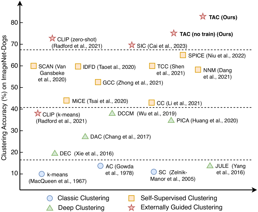
Figure 1: The evolution of clustering methods could be roughly divided into three eras, including i) classic clustering, which designs clustering strategies based on data distribution assumptions; ii) deep clustering, which extracts clustering-favorable features with deep neural networks by formulating clustering objectives as loss functions, and iii) self-supervised clustering, which constructs supervision signals through data augmentations or momentum strategies. As shown in the figure, each era remarkably improves the clustering accuracy. In this work, instead of mining the internal supervision, we propose exploring external knowledge to facilitate image clustering. We categorize such a novel paradigm as iv) externally guided clustering. By leveraging the semantics in the text modality, our TAC pushes the clustering accuracy to state-of-the-art with a remarkable improvement.

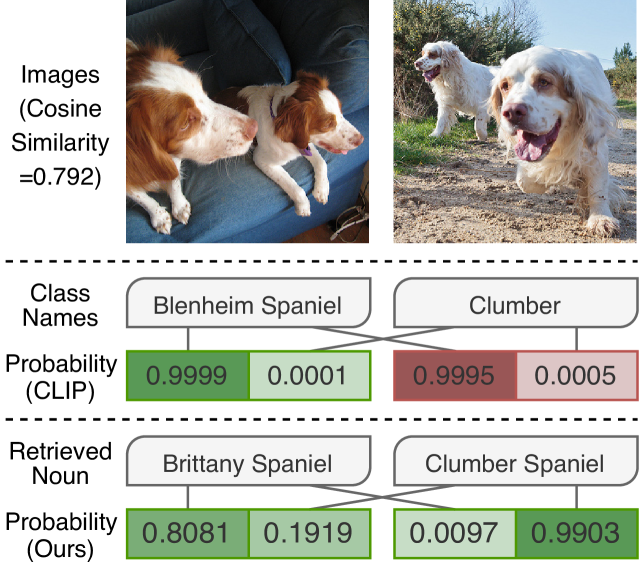
Figure 2: The observations of this paper. As a showcase, two image examples from the ImageNet-Dogs dataset are illustrated. For each example, we show the manually annotated class names and the nouns obtained by the proposed TAC, as well as the zero-shot classification probabilities. From the example, one could arrive at two observations, namely, i) visually similar samples could be better distinguished in the text modality, and ii) manually annotated class names are not always the best semantic description. As shown, zero-shot CLIP falsely classifies both images to the “Blenheim Spaniel” class, whereas the nouns obtained by our TAC successfully separate them. Such an observation suggests a great opportunity to leverage the external knowledge (hidden in the text modality in this showcase) to facilitate image clustering.

Though varying in the method design, most existing clustering methods design supervision signals in an internal manner. Despite the remarkable success achieved, the internally guided clustering paradigm faces an inherent limitation. Specifically, the hand-crafted internal supervision signals, even enhanced with data augmentation, are inherently upper-bounded by the limited information in the given data. For example, from the images of “penguins” and “polar bears”, one can hardly distinguish them based on living spaces given the similar image backgrounds. Luckily, beyond the internal signals, we notice there also exists well-established external knowledge that potentially conduces to clustering, while having been regrettably and largely ignored. In the above example, we could easily distinguish the images according to the living spaces, given the external knowledge that “penguins” live in the Antarctic while “polar bears” live in the Arctic. In short, from different sources or modalities, the external knowledge can serve as promising supervision signals to guide clustering, even though it seems irrelevant to the given data. Compared with exhaustively mining internal supervision signals from data, it would yield twice the effect with half the effort by incorporating rich and readily available external knowledge to guide clustering.

In this work, we propose a simple yet effective externally guided clustering method TAC (Text-Aided Clustering), which clusters images by incorporating external knowledge from the text modality. In the absence of class name priors, there are two challenges in leveraging the textual semantics for image clustering, namely, i) how to construct the text space, and ii) how to collaborate images and texts for clustering. For the first challenge, ideally, we expect the text counterparts of between-class images to be highly distinguishable so that clustering can be easily achieved. To this end, inspired by the zero-shot classification paradigm in CLIP [36], we reversely classify all nouns from WordNet [37] to image semantic centers. Based on the classification confidence, we select the most discriminative nouns for each image center to form the text space and retrieve a text counterpart for each image. Intriguingly, Fig. 2 demonstrates that in certain cases, the retrieved nouns could describe the image semantics even better than the manually annotated class names. For the second challenge, we first establish an extremely simple baseline by concatenating the images and text counterparts, which already significantly enhances the k-means clustering performance without any additional training. For better collaboration, we propose to mutually distill the neighborhood information between the text and image modalities. By specifically training clustering heads, the proposed TAC achieves state-of-the-art performance on five widely used and three more challenging image clustering datasets. Without loss of generality, we evaluate TAC on the pre-trained CLIP model in our experiments, but TAC could adapt to any vision-language pre-trained (VLP) model by design.

The major contributions of this work could be summarized as follows:

• Unlike previous clustering works that exhaustively explore and exploit supervision signals internally, we propose leveraging external knowledge to facilitate clustering. We summarize such a novel paradigm as externally guided clustering, which provides an innovative perspective on the construction of supervision signals.

• To implement and validate our idea, we propose an externally guided clustering method TAC, which leverages the textual semantics to facilitate image clustering. Experiments demonstrate the superiority of TAC over eight datasets, including ImageNet-1K. Impressively, in most cases, TAC even outperforms zero-shot CLIP in the absence of class name priors.

• The significance of TAC is two-fold. On the one hand, it proves the effectiveness and superiority of the proposed externally guided clustering paradigm. On the other hand, it suggests the presence of more simple but effective strategies for mining the zero-shot learning ability inherent in VLP models.

2 Related Work

In this section, we first review the deep clustering methods. Then we briefly introduce the zero-shot classification paradigm of VLP models which also utilizes the text modality to perform visual tasks.

2.1 Deep Image Clustering

In addition to effective clustering strategies, discriminative features also play an important role in achieving promising clustering results. Benefiting from the powerful feature extraction ability of neural networks, deep clustering methods show their superiority in handling complex and high-dimensional data [12, 14, 21]. The pioneers in deep clustering focus on learning clustering-favorable features through optimizing the network with clustering objectives [13, 16, 15, 22, 20, 38]. In recent years, motivated by the success of contrastive learning, a series of contrastive clustering methods achieve substantial performance leaps on image clustering benchmarks [26, 29, 34]. Instead of clustering images in an end-to-end manner, several works initially learn image embedding through uni-modal pre-training and subsequently mine clusters based on neighborhood consistency [30, 31] or pseudo-labeling [32]. By disentangling representation learning and clustering, these multi-stage methods enjoy higher flexibility for their easy adaption to superior pre-trained models. A recent study [35] demonstrates that the clustering performance could be further improved when equipping clustering models with more advanced representation learning methods [25]. Very recently, SIC [39] attempts to generate image pseudo labels from the textual space.

Though having achieved remarkable progressions, almost all existing deep image clustering methods mine supervision signals internally. However, the internal supervision signals are inherently bounded by the given images. Instead of pursuing internal supervision signals following previous works, we propose a new paradigm that leverages external knowledge to facilitate image clustering. Diverging from the most related work SIC that solely computes text semantic centers for pseudo labeling, our TAC retrieves discriminative text counterparts for mutual distillation. In addition, while SIC requires elaborate parameter tuning on different datasets, our TAC achieves promising results on all eight datasets with the same set of hyper-parameters, except the distillation temperature for large cluster numbers. We hope the simple design and engaging performance of TAC could attract more attention to the externally guided clustering.

2.2 Zero-shot Classification

Recently, more and more efforts have been devoted to multi-modal, especially vision-language pre-training (VLP). By learning the abundant image-text pairs on the Internet, VLP methods [40, 41, 42], with CLIP [36] as a representative, have achieved impressive performance in multi-modal representation learning. More importantly, unlike uni-modal pre-trained models that require additional fine-tuning, VLP models could adapt to various tasks such as classification [36], segmentation [43], and image captioning [42] in a zero-shot manner. Here, we briefly introduce the zero-shot image classification paradigm in CLIP as an example. Given names of $K$ classes such as “plane”, “train” or “car”, CLIP first assembles them with prompts like “a photo of [CLASS]”, where the [CLASS] token is replaced by the specific class name. Then, CLIP computes the text embeddings $\{w_{i}\}_{i=1}^{K}$ of the prompted sentences with its pre-trained text encoder. Finally, CLIP treats the embeddings $\{w_{i}\}_{i=1}^{K}$ as the weight of the classifier, and predicts the probability of image v belonging to the $i$-th class as

$$p(y=i|\textbf{v})=\frac{\exp(\operatorname{sim}(v,w_{i})/\tau)}{\sum_{j=1}^{K}\exp(\operatorname{sim}(v,w_{j})/\tau)},$$ (1)

where $v$ denotes the image features extracted by the pre-trained image encoder, and $\tau$ is the learned softmax temperature.

As CLIP is trained to retrieve the most correlated text for each image, its consistent form between pre-training and inference leads to promising results in zero-shot image classification. However, such a paradigm requires prior knowledge of class names, which is unavailable in the image clustering task. To leverage CLIP for image clustering, the most direct approach is performing k-means [1] on the image embeddings. Nevertheless, the performance of k-means is limited and the textual semantics are underutilized. In this work, we explore a more advanced paradigm for image clustering, by taking full advantage of both the pre-trained image and text encoders. Briefly, we construct a text counterpart for each image by retrieving nouns that best distinguish images of different semantics, which significantly improves the feature discriminability. To collaborate the text and image modalities, we propose to mutually distill cross-modal neighborhood information, which further improves the clustering performance. Intriguingly, our experiments demonstrate that the proposed method outperforms zero-shot CLIP in most cases, even in the absence of class name priors. We believe such intriguing results could bring some insights into the paradigm design of leveraging VLP models for downstream classification and clustering.

Figure 3: Overview of the proposed TAC. (Left) TAC first classifies all nouns from WordNet to image semantic centers, and selects the most discriminative nouns of each image center to construct the text space. After that, TAC retrieves nouns for each image to compute its counterpart in the text space. By concatenating the image and retrieved text, we arrive at an extremely simple baseline with significantly improved k-means performance. (Right) To better collaborate the text and image modalities, TAC trains cluster heads by mutually distilling the neighborhood information. In brief, TAC encourages images to have consistent cluster assignments with the nearest neighbors of their counterparts in the text embedding space, and vice versa. Such a cross-modal mutual distillation strategy further boosts the clustering performance of TAC.

3 Method

In this section, we present TAC, a simple yet effective externally supervised clustering method. The overview of TAC is illustrated in Fig. 3. In brief, we first propose a text counterpart construction strategy to exploit the text modality in Sec. 3.1. By selecting and retrieving discriminative nouns for each image, TAC yields an extremely simple baseline that significantly improves the k-means performance at negligible cost. To better collaborate the text and image modalities, in Sec. 3.2, we propose a cross-modal mutual distillation strategy to train cluster heads in both modalities, further improving the clustering performance.

3.1 Text Counterpart Construction

The textual semantics are naturally favored in discriminative tasks such as classification and clustering. Ideally, clustering could be easily achieved if images have highly distinguishable counterparts in the text modality. To this end, in the absence of class name priors, we propose to select a subset of nouns from WordNet [37] to compose the text space, which is expected to exhibit the following two merits, namely, i) precisely covering the image semantics; and ii) highly distinguishable between images of different semantics.

The image semantics of different granularities could be captured by k-means with various choices of $k$. A small value of $k$ corresponds to coarse-grained semantics, which might not be precise enough to cover the semantics of images at cluster boundaries. Oppositely, a large value of $k$ produces fine-grained semantics, which might fail to distinguish images from different classes. To find image semantics of appropriate granularity, we estimate the value of $k$ based on the data number $N$ and target cluster number $K$, namely,

$$k=\max\{N/300,K*3\}.$$ (2)

The motivation behind such an estimation is two-fold. On the one hand, for large datasets, we hypothesize a cluster of $\tilde{N}=300$ images is compact enough to be described by the same set of nouns. On the other hand, for small datasets, we hypothesize the semantics of images from one class could be precisely covered by three sets of nouns. In our experiments, such estimation works on datasets of different sample sizes and target cluster numbers. With the estimated value of $k$, we apply k-means on image embeddings to compute the image semantic centers by

$$s_{l}=\sum_{i=1}^{N}\mathbbm{1}_{v_{i}\in l}~{}v_{i},l\in[1,k],$$ (3)

where $\mathbbm{1}_{v_{i}\in l}$ is the indicator which equals one iff image $v_{i}$ belongs to the $l$-th cluster.

Next, we aim to find discriminative nouns to describe each semantic center. Here, motivated by the zero-shot classification paradigm of CLIP, we reversely classify all nouns from WordNet into $k$ image semantic centers. Specifically, the probability of the $i$-th noun belonging to the $l$-th image semantic center is

$$p(y=l|\mathbf{t_{i}})=\frac{\exp(\operatorname{sim}(t_{i},s_{l}))}{\sum_{j=1}^{k}\exp(\operatorname{sim}(t_{i},s_{j}))},$$ (4)

where $\mathbf{t_{i}}$ denoted the $i$-th noun prompted like CLIP, and $t_{i}$ is the feature extracted by the text encoder. To identify highly representative and distinguishable nouns, we select the top $\gamma$ confident nouns for each image semantic center. Formally, the $i$-th noun would be select for the $l$-th center if

$$p(y=k|\mathbf{t_{i}})\geq\bar{p}(y=k),$$ (5)

$$\bar{p}(y=k)=\operatorname{sort}\{p(y=k|\mathbf{t_{i}})|\operatorname{argmax}p(y|\mathbf{t_{i}})=k\}[\gamma],$$ (6)

where $\bar{p}(y=k)$ corresponds to the $\gamma$-th largest confidence of nouns belonging to the $l$-th center. In practice, we fix $\gamma=5$ on all datasets.

The selected nouns compose the text space catering to the input images. Then, we retrieve nouns for each image to compute its counterpart in the text modality. To be specific, let $\{\mathbf{\bar{t}_{i}}\}_{i=1}^{M}$ be the set of $M$ selected nouns with $\{\bar{t}_{i}\}_{i=1}^{M}$ being their text embeddings, we compute the text counterpart $\tilde{t}_{i}$ for image $v_{i}$ as

$$\tilde{t}_{i}=\sum_{j=1}^{M}p(\bar{t}_{j}|v_{i})\bar{t}_{j},$$ (7)

$$p(\bar{t}_{j}|v_{i})=\frac{\exp(\operatorname{sim}(v_{i},\bar{t}_{j})/\tilde{\tau})}{\sum_{k=1}^{M}\exp(\operatorname{sim}(v_{i},\bar{t}_{k})/\tilde{\tau})},$$ (8)

where $\tilde{\tau}$ controls the softness of retrieval, which is fixed to $0.005$ in all our experiments. The design of soft retrieval is to prevent the text counterparts of different images from collapsing to the same point. After the text counterpart construction, we arrive at an extremely simple baseline by applying k-means on the concatenated features $[\tilde{t}_{i},v_{i}]_{i=1}^{N}$. Notably, such an implementation requires no additional training or modifications on CLIP, but it could significantly improve the clustering performance compared with directly applying k-means on the image embeddings.

Algorithm 1 The TAC method

Input: Images $\mathbf{V}$, VLP Image and Text Encoders $\Phi_{T}$ and $\Phi_{V}$, Cluster Heads $f$ and $g$, Cluster Number $K$.

Output: Cluster Assignments $\mathbf{Y}$.

// Prepare Image and Text Embeddings

Compute image embeddings via $V=\Phi_{V}(\mathbf{V})$.

Prompt nouns from WordNet $\mathbf{T}$ and compute text embeddings via $T=\Phi_{V}(\mathbf{T})$.

// Text Counterpart Construction

Compute image semantic centers via Eq. 3.

Classify $T$ into image semantic centers via Eq. 4.

Select discriminative nouns $\{\mathbf{\bar{t}_{i}}\}_{i=1}^{M}$ via Eq. 5 and 6.

Compute text counterparts $\{\tilde{t}_{i}\}_{i=1}^{N}$ via Eq. 7 and 8.

// TAC without Training

Perform k-means on the concatenated embeddings $[\tilde{t}_{i},v_{i}]_{i=1}^{N}$ with $k$ estimated by Eq. 2 to obtain $\mathbf{Y}$.

// Cross-modal Mutual Distillation

while not converge do

       Sample batch of samples $\{\tilde{t}_{i}\}_{i=1}^{n}$ and $\{v_{i}\}_{i=1}^{n}$. Sample neighbors $\{\mathcal{N}(\tilde{t}_{i})\}_{i=1}^{n}$ and $\{\mathcal{N}(v_{i})\}_{i=1}^{n}$. Compute cluster assignment matrices $P,P^{\mathcal{N}},Q,Q^{\mathcal{N}}$ via Eq. 9 and 10. Compute the cross-modal mutual distillation loss $L_{\mathrm{Dis}}$ via Eq. 11–13. Compute the confidence loss $L_{\mathrm{Con}}$ via Eq. 14. Compute the balance loss $L_{\mathrm{Bal}}$ via Eq. 15–16. Update cluster heads $f$ and $g$ through gradient descent to minimize the overall loss $L_{\mathrm{TAC}}$ in Eq. 17.

end while

Compute cluster assignments $\mathbf{Y}=\operatorname{argmax}f(V)$.

3.2 Cross-modal Mutual Distillation

Though concatenating text counterparts and image embeddings improves the k-means performance, it is suboptimal for collaborating the two modalities. To better utilize multi-modal features, we propose the cross-modal mutual distillation strategy. Specifically, let $\mathcal{N}(v_{i})$ be a random nearest neighbor of $v_{i}$, we introduce a cluster head $f:v\rightarrow p\in\mathcal{R}^{K}$ to predict the soft cluster assignments for images $v_{i}$ and $\mathcal{N}(v_{i})$, where $K$ is the target cluster number. Formally, we denote the soft cluster assignments for $n$ images and their neighbors as

$$P=\left[\begin{array}[]{c}p_{1}\\ \cdots\\ p_{n}\end{array}\right]\text{ and }P^{\mathcal{N}}=\left[\begin{array}[]{c}p^{\mathcal{N}}_{1}\\ \cdots\\ p^{\mathcal{N}}_{n}\end{array}\right].$$ (9)

Likewise, we introduce another cluster head $g:\tilde{t}_{i}\rightarrow q_{i}\in\mathcal{R}^{K}$ to predict the soft cluster assignments for text counterpart $\tilde{t}_{i}$ and its random nearest neighbor $\mathcal{N}(\tilde{t}_{i})$, resulting in the cluster assignment matrices

$$Q=\left[\begin{array}[]{c}q_{1}\\ \cdots\\ q_{n}\end{array}\right]\text{ and }Q^{\mathcal{N}}=\left[\begin{array}[]{c}q^{\mathcal{N}}_{1}\\ \cdots\\ q^{\mathcal{N}}_{n}\end{array}\right].$$ (10)

Let $\hat{p}_{i},\hat{p}^{\mathcal{N}}_{i},\hat{q}_{i},\hat{q}^{\mathcal{N}}_{i}$ be the $i$-th column of assignment matrices $P,P^{\mathcal{N}},Q,Q^{\mathcal{N}}$, the cross-modal mutual distillation loss is defined as follows, namely,

$$L_{\mathrm{Dis}}=\sum_{i=1}^{K}L^{v\rightarrow t}_{i}+L^{t\rightarrow v}_{i},$$ (11)

$$L^{v\rightarrow t}_{i}=-\log\frac{\exp(\operatorname{sim}(\hat{q}_{i},\hat{p}^{\mathcal{N}}_{i})/\hat{\tau})}{\sum_{k=1}^{K}\exp(\operatorname{sim}(\hat{q}_{i},\hat{p}^{\mathcal{N}}_{k})/\hat{\tau})},$$ (12)

$$L^{t\rightarrow v}_{i}=-\log\frac{\exp(\operatorname{sim}(\hat{p}_{i},\hat{q}^{\mathcal{N}}_{i})/\hat{\tau})}{\sum_{k=1}^{K}\exp(\operatorname{sim}(\hat{p}_{i},\hat{q}^{\mathcal{N}}_{k})/\hat{\tau})},$$ (13)

where $\hat{\tau}$ is the softmax temperature parameter. The distillation loss $L_{\mathrm{Dis}}$ has two effects. On the one hand, it minimizes the between-cluster similarity, leading to more discriminative clusters. On the other hand, it encourages consistent clustering assignments between each image and the neighbors of its text counterpart, and vice versa. In other words, it mutually distills the neighborhood information between the text and image modalities, bootstrapping the clustering performance in both. In practice, we set the number of nearest neighbors $\hat{N}=50$ on all datasets.

Next, we introduce two regularization terms to stabilize the training. First, to encourage the model to produce more confident cluster assignments, we introduce the following confidence loss, namely,

$$L_{\mathrm{Con}}=-\log\sum_{i=1}^{n}p_{i}^{\top}q_{i},$$ (14)

which would be minimized when both $p_{i}$ and $q_{i}$ become one-hot. Second, to prevent all samples from collapsing into only a few clusters, we introduce the following balance loss, i.e.,

$$L_{\mathrm{Bal}}=-\sum_{i=1}^{K}\left(\bar{p}_{i}\log\bar{p}_{i}+\bar{q}_{i}\log\bar{q}_{i}\right),$$ (15)

$$\bar{p}=\frac{1}{n}\sum_{i=1}^{n}p_{i}\in\mathcal{R}^{K},\bar{q}=\frac{1}{n}\sum_{i=1}^{n}q_{i}\in\mathcal{R}^{K},$$ (16)

where $\bar{p}$ and $\bar{q}$ correspond to the cluster assignment distribution in the image and text modality, respectively.

Finally, we arrive at the overall objective function of TAC, which lies in the form of

$$L_{\mathrm{TAC}}=L_{\mathrm{Dis}}+L_{\mathrm{Con}}-\alpha\cdot L_{\mathrm{Bal}},$$ (17)

where $\alpha$ is the weight parameter which we fix to 5 in all the experiments.

The pipeline of the proposed TAC is summarized in Algorithm 1, including the simple baseline without training and the full version with cross-modal mutual distillation.

4 Experiments

In this section, we evaluate the proposed TAC on five widely used and three more challenging image clustering datasets. A series of quantitative and qualitative comparisons, ablation studies, and hyper-parameter analyses are carried out to investigate the effectiveness and robustness of the method.

4.1 Experimental Setup

We first introduce the datasets and metrics used for evaluation, and then provide the implementation details of TAC.

TABLE I: A summary of datasets used for evaluation.

Dataset	Training Split	Test Split	# Training	# Test	# Classes
STL-10	Train	Test	5,000	8,000	10
CIFAR-10	Train	Test	50,000	10,000	10
CIFAR-20	Train	Test	50,000	10,000	20
ImageNet-10	Train	Val	13,000	500	10
ImageNet-Dogs	Train	Val	19,500	750	15
DTD	Train+Val	Test	3,760	1,880	47
UCF-101	Train	Val	9,537	3.783	101
ImageNet-1K	Train	Val	1,281,167	50,000	1,000

TABLE II: Clustering performance on five widely-used image clustering datasets. The bottom five rows correspond to methods leveraging pre-trained CLIP. The best and second best results are denoted in bold and underline, respectively.

Dataset	STL-10			CIFAR-10			CIFAR-20			ImageNet-10			ImageNet-Dogs			AVG
Metrics	NMI	ACC	ARI	NMI	ACC	ARI	NMI	ACC	ARI	NMI	ACC	ARI	NMI	ACC	ARI
JULE	18.2	27.7	16.4	19.2	27.2	13.8	10.3	13.7	3.3	17.5	30.0	13.8	5.4	13.8	2.8	15.5
DEC	27.6	35.9	18.6	25.7	30.1	16.1	13.6	18.5	5.0	28.2	38.1	20.3	12.2	19.5	7.9	21.2
DAC	36.6	47.0	25.7	39.6	52.2	30.6	18.5	23.8	8.8	39.4	52.7	30.2	21.9	27.5	11.1	31.0
DCCM	37.6	48.2	26.2	49.6	62.3	40.8	28.5	32.7	17.3	60.8	71.0	55.5	32.1	38.3	18.2	41.3
IIC	49.6	59.6	39.7	51.3	61.7	41.1	22.5	25.7	11.7	–	–	–	–	–	–	–
PICA	61.1	71.3	53.1	59.1	69.6	51.2	31.0	33.7	17.1	80.2	87.0	76.1	35.2	35.3	20.1	52.1
CC	76.4	85.0	72.6	70.5	79.0	63.7	43.1	42.9	26.6	85.9	89.3	82.2	44.5	42.9	27.4	62.1
IDFD	64.3	75.6	57.5	71.1	81.5	66.3	42.6	42.5	26.4	89.8	95.4	90.1	54.6	59.1	41.3	63.9
MiCE	63.5	75.2	57.5	73.7	83.5	69.8	43.6	44.0	28.0	–	–	–	42.3	43.9	28.6	–
GCC	68.4	78.8	63.1	76.4	85.6	72.8	47.2	47.2	30.5	84.2	90.1	82.2	49.0	52.6	36.2	64.3
NNM	66.3	76.8	59.6	73.7	83.7	69.4	48.0	45.9	30.2	–	–	–	60.4	58.6	44.9	–
TCC	73.2	81.4	68.9	79.0	90.6	73.3	47.9	49.1	31.2	84.8	89.7	82.5	55.4	59.5	41.7	67.2
SPICE	81.7	90.8	81.2	73.4	83.8	70.5	44.8	46.8	29.4	82.8	92.1	83.6	57.2	64.6	47.9	68.7
SCAN	69.8	80.9	64.6	79.7	88.3	77.2	48.6	50.7	33.3	–	–	–	61.2	59.3	45.7	–
CLIP (k-means)	91.7	94.3	89.1	70.3	74.2	61.6	49.9	45.5	28.3	96.9	98.2	96.1	39.8	38.1	20.1	66.3
TAC (no train)	92.3	94.5	89.5	80.8	90.1	79.8	60.7	55.8	42.7	97.5	98.6	97.0	75.1	75.1	63.6	79.5
CLIP (zero-shot)	93.9	97.1	93.7	80.7	90.0	79.3	55.3	58.3	39.8	95.8	97.6	94.9	73.5	72.8	58.2	78.7
SIC	95.3	98.1	95.9	84.7	92.6	84.4	59.3	58.3	43.9	97.0	98.2	96.1	69.0	69.7	55.8	79.9
TAC	95.5	98.2	96.1	84.1	92.3	83.9	61.1	60.7	44.8	98.5	99.2	98.3	80.6	83.0	72.2	83.2

4.1.1 Datasets

To evaluate the performance of our TAC, we first apply it to five widely-used image clustering datasets including STL-10 [44], CIFAR-10 [45], CIFAR-20 [45], ImageNet-10 [46], and ImageNet-Dogs [46]. With the rapid development of pre-training and clustering methods, we find clustering on relatively simple datasets such as STL-10 and CIFAR-10 is no longer challenging. Thus, we further evaluate the proposed TAC on three more complex datasets with larger cluster numbers, including DTD [47], UCF-101 [48], and ImageNet-1K [49]. Following recent deep clustering works [30, 31], we train and evaluate TAC on the train and test splits, respectively. The brief information of all datasets used in our evaluation is summarized in Table I.

4.1.2 Evaluation metrics

We adopt three widely-used clustering metrics including Normalized Mutual Information (NMI) [50], Accuracy (ACC), and Adjusted Rand Index (ARI) [51] to evaluate the clustering performance. Higher values of these metrics indicate better clustering results.

4.1.3 Implementation details

Following previous works [39], we adopt the pre-trained CLIP model with ViT-B/32 [52] and Transformer [53] as image and text backbones, respectively. Consistent with the CLIP preprocessing pipeline, we scale, random crop, and normalize images before feeding them into the ViT backbone. For nouns from WordNet [37], we assemble them with prompts like “A photo of [CLASS]” before feeding them into the Transformer backbone. The two cluster heads $f$ and $g$ are two-layer MLPs of dimension $512$-$512$-$K$, where $K$ is the target cluster number. We train $f$ and $g$ by the Adam optimizer with an initial learning rate of $1e{-3}$ for $20$ epochs, with a batch size of $512$. We fix $\tau=5e{-3}$, $\hat{\tau}=0.5$, and $\alpha=5.0$ in all the experiments. The only exception is that on UCF-101 and ImageNet-1K, we change $\hat{\tau}$ to $5.0$, batch size to $8192$, and training epochs to $100$, catering to the large cluster number. We evaluate TAC under five random runs and report the average performance. All experiments are conducted on a single Nvidia RTX 3090 GPU on the Ubuntu 20.04 platform with CUDA 11.4. In our experiments, it takes only one minute to train TAC on the CIFAR-10 dataset.

4.2 Main Results

Here we compare TAC with state-of-the-art baselines on five classic and three more challenging image clustering datasets, followed by feature visualizations to show the superiority of the proposed TAC.

4.2.1 Performance on classic clustering datasets

We first evaluate the proposed TAC on five widely-used image clustering datasets, compared with 15 deep clustering baselines including JULE [13], DEC [16], DAC [17], DCCM [18], IIC [38], PICA [20], CC [26], IDFD [28], MiCE [27], GCC [34], NNM [31], TCC [29], SPICE [32], SCAN [30], and SIC [39]. In addition, we include two CLIP [36] baselines, namely, k-means on image embeddings and zero-shot classification that requires prior knowledge of class names.

As shown in Table II, by simply retrieving a text counterpart for each image, the proposed TAC successfully mines “free” semantic information from the text encoder. Without any additional training, TAC (no train) substantially improves the k-means clustering performance, especially on more complex datasets. For example, it achieves 14.4% and 43.5% ARI improvements on CIFAR-20 and ImageNet-Dogs, respectively. When further enhanced with the proposed cross-modal mutual distillation strategy, TAC achieves state-of-the-art clustering performance, even surpassing zero-shot CLIP on all five datasets. Notably, the improvement brought by leveraging the text modality is significant on ImageNet-Dogs, demonstrating the potential of texts in distinguishing visually similar samples. Such compelling results demonstrate that beyond the current zero-shot classification paradigm, alternative simple but more effective strategies exist for mining the VLP model’s ability in image classification and clustering.

TABLE III: Clustering performance on three more challenging image clustering datasets. The best and second best results are denoted
in bold and underline, respectively. ${\dagger}$ means that using prior class names instead of nouns selected from WordNet.

Dataset	DTD			UCF-101			ImageNet-1K			AVG
Metrics	NMI	ACC	ARI	NMI	ACC	ARI	NMI	ACC	ARI
CLIP (k-means)	57.3	42.6	27.4	79.5	58.2	47.6	72.3	38.9	27.1	50.1
TAC (no train)	60.1	45.9	29.0	81.6	61.3	52.4	77.8	48.9	36.4	54.8
CLIP (zero-shot)	56.5	43.1	26.9	79.9	63.4	50.2	81.0	63.6	45.4	56.7
SCAN	59.4	46.4	31.7	79.7	61.1	53.1	74.7	44.7	32.4	53.7
SIC	59.6	45.9	30.5	81.0	61.9	53.6	77.2	47.0	34.3	54.6
TAC	62.1	50.1	34.4	82.3	68.7	60.1	79.9	58.2	43.5	59.9
TAC†	60.8	48.0	32.6	83.0	71.3	61.9	81.2	63.9	47.0	61.1

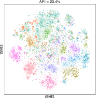
(a) CLIP Image Embedding

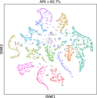
(b) Constructed Text Counterpart

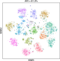
(c) TAC (no train)

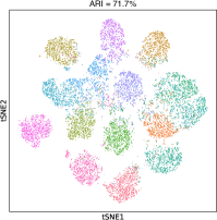
(d) TAC

Figure 4: Visualization of features extracted by different methods on the ImageNet-Dogs training set, with the corresponding k-means clustering ARI annotated on the top. a) image embedding directly obtained from the CLIP image encoder; b) text counterparts constructed by noun selection and retrieval; c) the simple TAC baseline by concatenating images and text counterparts; d) representation learned by TAC through cross-modal mutual distillation.

4.2.2 Performance on more challenging datasets

We note that with the advance of pre-training and clustering methods, some classic datasets are no longer challenging enough for clustering. For example, our TAC achieves 98.2% and 99.2% clustering accuracy on STL-10 and ImageNet-10, respectively. Persistently pursuing performance gain on these relatively simple datasets might fall into the over-fitting trap, leading to poor generalization ability of clustering methods, which is also unhealthy for the clustering community development. Hence, we further introduce three more challenging image clustering datasets for benchmarking. We include two representative baselines SCAN [30] and SIC [39] for comparison. For SCAN, we replace its first pre-training step with the pre-trained CLIP image encoder, and use its semantic clustering loss to train the cluster head. For SIC, as its source code is not released, we reimplement it following the details provided in the paper. Moreover, we also include the k-means and zero-shot performance of CLIP for benchmarking.

The clustering results of TAC and baseline methods are provided in Table III. Firstly, we observe TAC without additional training could consistently boost the k-means performance, which achieves a 10% improvement in clustering accuracy on ImageNet-1K. Secondly, with the cross-modal mutual distillation strategy, TAC outperforms zero-shot CLIP and achieves the best clustering results on DTD and UCF-101. For example, compared with SCAN which solely mines clusters from the image modality, our TAC exhibits a 7.6% accuracy gain on UCF-101 by exploiting the textual semantics. Compared with the previous CLIP-based image clustering method SIC, our TAC also outperforms it by 6.8% in accuracy, demonstrating the superiority of the proposed paradigm. On the largest dataset ImageNet-1K, our TAC outperforms SCAN and SIC even without additional training, and the performance gap in clustering accuracy increases to 13.5% and 11.2% when TAC is further boosted with the proposed cross-modal mutual distillation strategy. Notably, the zero-shot CLIP yields better performance than our TAC on ImageNet-1K, given its advantage in the substantial prior knowledge of 1K class names. We further evaluate our TAC by replacing the selected discriminative nouns with prior class names. The results show that TAC successfully outperforms zero-shot CLIP when leveraging the class name priors, which demonstrates the superior zero-shot classification ability of TAC. Notably, TAC achieves inferior performance with the prior class names than retrieved nouns on the DTD dataset. Such a result verifies the effectiveness of the proposed text counterpart construction strategy, as well as our observation that manually annotated class names are not always the best semantic description.

4.2.3 Visualization

To provide an intuitive understanding of the clustering results, we visualize the features obtained at four different steps of TAC in Fig. 4. The clustering performance by applying k-means on the features is annotated at the top. Fig. 4(a) shows the image features extracted by the pre-trained CLIP image encoder. As can be seen, images of different breeds of dogs are mixed, leading to a poor clustering ARI of 23.4%. Luckily, by selecting and retrieving discriminative nouns, we can construct discriminative text counterparts for images. Thanks to the textual discriminability, visually similar samples could be better distinguished in the text modality as shown in Fig. 4(b). As shown in Fig. 4(c), by simply concatenating images and retrieved text counterparts, TAC significantly improves the feature discriminability without any additional training, yielding a promising clustering ARI of 61.3%. Finally, when equipped with the proposed cross-modal mutual distillation strategy, TAC could better collaborate the image and text modalities, leading to the best clustering ARI of 71.7%. We visualize the embedding learned by TAC before the softmax layer in Fig. 4(d), which shows the best within-clustering compactness and between-cluster scatteredness.

4.3 Ablation Studies

To prove the robustness, effectiveness, and generalization ability of the proposed TAC, we conduct ablation studies on text counterpart construction strategies, loss terms, and image backbones.

4.3.1 Variants of text counterpart construction

Recall that to select representation nouns for text counterpart construction, we first classify all nouns from WordNet to image semantic centers found by applying k-means on image embeddings. Here, we investigate the robustness and necessity of the noun selection step. Specifically, we adopt three other classic clustering methods to compute semantic centers, including agglomerative clustering (AC), spectral clustering (SC), and DBSCAN. For AC and SC, we set the target cluster number to the same as k-means (estimated by Eq. 2). For DBSCAN, we tune the density parameter until it produces the same number of clusters. As shown in Table IV, the training-free TAC achieves better performance with SC, while the performance is similar among k-means, AC, and SC when further boosted with cross-modal mutual distillation. The performance degradation on DBSCAN is probably due to the poor quality of image embeddings. In practice, we find DBSCAN tends to treat a portion of samples as outliers, and thus it cannot precisely cover the image semantics, leading to suboptimal performance. To investigate the necessity to filter discriminative nouns, we further append a baseline by retrieving text counterparts from all nouns. According to the results, TAC encounters a performance drop on both datasets, but the influence is milder on UCF-101, which could be attributed to the richer image semantics in that dataset. In summary, the results demonstrate the effectiveness of discriminative noun selection, as well as the robustness of TAC against different clustering methods used for text counterpart construction.

TABLE IV: Clustering performance of TAC using different clustering methods for text counterpart construction. (AC: agglomerative clustering, SC: spectral clustering, None: using all nouns from WordNet)

Method	Semantic Space	ImageNet-Dogs			UCF-101
		NMI	ACC	ARI	NMI	ACC	ARI
TAC (no train)	k-means	75.1	75.1	63.6	81.6	61.3	52.4
	AC	73.4	72.0	61.2	81.9	63.7	54.8
	SC	77.4	75.2	65.9	82.2	65.5	54.7
	DBSCAN	68.8	64.3	51.0	81.1	61.8	52.3
	None	70.3	68.7	53.6	81.3	63.2	52.8
TAC	k-means	80.6	83.0	72.2	82.3	68.7	60.1
	AC	78.4	81.7	69.5	82.4	69.3	60.2
	SC	79.2	83.1	70.8	82.3	69.1	60.4
	DBSCAN	75.5	80.4	65.5	80.6	66.2	56.4
	None	75.7	78.7	66.0	81.2	67.0	58.3

4.3.2 Effectiveness of each loss term

To understand the efficacy of the three loss terms $L_{\mathrm{Dis}}$, $L_{\mathrm{Con}}$, and $L_{\mathrm{Bal}}$ in Eq. 11, 14, and 15, we evaluate the performance of TAC with different loss combinations. According to the results in Table V, we arrive at the following four conclusions. First, each loss itself is not sufficient to produce good clustering results. Second, the balance loss $L_{\mathrm{Bal}}$ could prevent cluster collapsing. Without $L_{\mathrm{Bal}}$, TAC assigns most images to only a few clusters, leading to poor clustering performance on both datasets. Third, the confidence loss $L_{\mathrm{Con}}$ is necessary for datasets with large cluster numbers. Without $L_{\mathrm{Con}}$, TAC can still achieve promising results on ImageNet-Dogs but encounters a performance drop on UCF-101. The reason is that the cluster assignments would be less confident when the cluster number is large. In this case, the regularization efficacy of $L_{\mathrm{Bal}}$ would be alleviated, which explains the performance degradation on UCF-101. Fourth, $L_{\mathrm{Dis}}$ could effectively distill the neighborhood information between the text and image modalities, leading to the best clustering performance.

TABLE V: The performance of TAC with different combinations of the loss terms.

$L_{\mathrm{Dis}}$	$L_{\mathrm{Con}}$	$L_{\mathrm{Bal}}$	ImageNet-Dogs			UCF-101
			NMI	ACC	ARI	NMI	ACC	ARI
✓			71.4	69.5	38.1	69.3	7.6	13.6
	✓		57.2	14.3	24.3	52.1	3.4	8.6
		✓	15.1	19.3	4.1	43.5	16.2	5.7
✓	✓		72.5	57.0	45.3	55.6	3.6	9.9
✓		✓	80.6	83.5	72.3	70.5	45.1	34.5
	✓	✓	78.2	81.8	69.6	81.6	67.3	59.1
✓	✓	✓	80.6	83.0	72.2	82.3	68.7	60.1

4.3.3 Variants of CLIP image backbones

In our experiments, for a fair comparison with previous works [39], we adopt ViT-B/32 as the image backbone. Here, to investigate whether the proposed TAC generalizes to other backbones, we further evaluate its performance on ResNet-50, ResNet-101, and ViT-B/16. We also report the k-means and zero-shot performance of CLIP for comparison. As shown in Table VI, the performance of TAC is positively correlated with the size of image backbones. On all four image backbones, TAC achieves comparable performance with zero-shot CLIP without any additional training, modifications on the CLIP, or prior knowledge of class names. When further enhanced with cross-modal mutual distillation, TAC outperforms zero-shot CLIP in all cases. The promising results prove the generalization ability of our TAC to various image backbones.

TABLE VI: The clustering performance of TAC and CLIP variations with different image backbones.

Method	Backbone	ImageNet-Dogs			UCF101			AVG
		NMI	ACC	ARI	NMI	ACC	ARI
CLIP (k-means)	ResNet-50	35.3	35.2	18.9	75.9	53.5	42.6	43.6
	ResNet-101	50.5	47.9	32.9	78.5	56.3	46.3	52.1
	ViT-B/32	39.8	38.1	20.1	79.5	58.2	47.6	47.2
	ViT-B/16	48.5	42.3	29.4	81.4	60.2	51.9	52.3
TAC (no train)	ResNet-50	75.5	74.7	62.6	76.1	55.7	44.4	64.8
	ResNet-101	76.8	74.0	62.8	77.9	59.1	48.8	66.5
	ViT-B/32	75.1	75.1	63.6	81.6	61.3	52.4	68.2
	ViT-B/16	81.3	80.8	71.2	82.5	63.3	54.8	72.3
CLIP (zero-shot)	ResNet-50	76.0	75.9	60.6	75.2	59.9	45.2	65.5
	ResNet-101	72.9	73.6	58.2	77.4	62.0	48.6	65.4
	ViT-B/32	73.5	72.8	58.2	79.9	63.4	50.2	66.3
	ViT-B/16	80.4	80.4	68.4	81.9	68.0	57.0	72.7
TAC	ResNet-50	76.1	79.8	66.6	76.3	60.6	49.3	68.1
	ResNet-101	79.1	81.4	70.6	79.8	66.2	56.1	72.2
	ViT-B/32	80.6	83.0	72.2	82.3	68.7	60.1	74.5
	ViT-B/16	82.1	85.7	74.5	83.3	70.4	61.8	76.3

4.4 Parameter Analyses

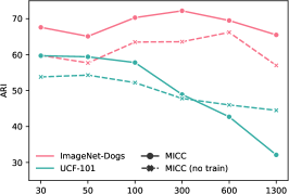
(a)    Expected compact cluster size $\tilde{N}$

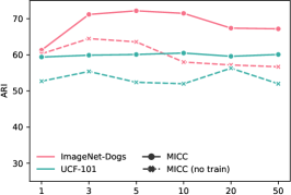
(b)    Number of discriminative nouns $\gamma$

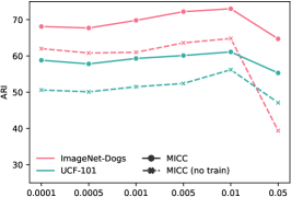
(c)    Retrieval softness temperature $\tilde{\tau}$

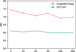
(d)    Number of nearest neighbors $\hat{N}$

(e)    Mutual distillation temperature $\hat{\tau}$

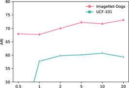
(f)    Weight of the entropy loss $\alpha$

Figure 5: Analyses on six tunable hyper-parameters in the proposed TAC. The first three hyper-parameters influence both TAC with and without training. The last three hyper-parameters only influence the cross-modal mutual distillation process of TAC.

Though we fix the set of hyper-parameters in all experiments except a larger $\hat{\tau}$ to handle large cluster number, there are six tunable hyper-parameters in TAC, namely, the expected compact cluster size $\tilde{N}$, the number of discriminative nouns for each image semantic center $\gamma$, the retrieval softness temperature $\tilde{\tau}$, the number of nearest neighbors $\hat{N}$, the mutual distillation temperature $\hat{\tau}$, and the weight of the balance loss $\alpha$. We evaluate the performance of TAC under various choices of these hyper-parameters on ImageNet-Dogs and UCF-101. The results are shown in Fig. 5.

4.4.1 Expected compact cluster size $\tilde{N}$

To capture semantics with appropriate granularity, we empirically hypothesize a cluster of $\tilde{N}=300$ images is compact enough to be described by the same set of nouns. Here, we test various choices of $\tilde{N}$ to see how the granularity of image semantics influences the final clustering performance. As shown in Fig. 5(a), TAC achieves inferior performance under large $\tilde{N}$ on both datasets. The reason is that under an excessively large cluster size, the semantics would be overly coarse-grained, thereby failing to precisely delineate the images at cluster boundaries. Conversely, when the cluster size is overly small, the excessively fine-grained semantics would break cluster structures, leading to performance degradation on ImageNet-Dogs. Notably, the proper range of $\tilde{N}$ is smaller on UCF-101 than ImageNet-Dogs, owing to the former’s richer image semantics. The results demonstrate the necessity and effectiveness of the proposed cluster number estimation criterion in Eq. 2.

4.4.2 Number of discriminative nouns $\gamma$

After computing image semantic centers, we classify all nouns into the centers and select the top $\gamma$ nouns of each center as discriminative nouns. We try various choices of $\gamma$, and the results are shown in Fig. 5(b). As can be seen, a solitary noun is insufficient to cover the semantics of each image center. Conversely, an excessive number of nouns would falsely enrich the semantics, leading to inferior performance. The results show that the performance of TAC is stable with discriminative noun number $\gamma$ in a typical range of 3–10.

4.4.3 Retrieval softness temperature $\tilde{\tau}$

Recall that we introduce a softness temperature $\tilde{\tau}$ when retrieving nouns to construct text counterparts. The smaller choice of $\tilde{\tau}$ leads to more discriminative text counterparts. However, when $\tilde{\tau}$ is too small, text counterparts of different images would collapse into the same noun, which damages the neighborhood information. As shown in Fig. 5(c), the clustering performance of TAC improves as the temperature $\tilde{\tau}$ increases to 0.01. However, continually increasing $\tilde{\tau}$ leads to a performance decrease, as samples of different semantics would be mixed in the text modality.

4.4.4 Number of nearest neighbors $\hat{N}$

To collaborate the text and image modalities, we propose to mutually distill their neighborhood information. Here, we evaluate the performance of TAC with different numbers of nearest neighbors $\bar{N}$ in Fig. 5(d). The results demonstrate that TAC is robust to diverse numbers of $\bar{N}$. In our experiments, we simply fix $\bar{N}=50$ on all datasets of varying sizes. However, we find the performance of TAC could be further boosted if $\bar{N}$ is delicately tuned.

4.4.5 Mutual distillation temperature $\hat{\tau}$

The mutual distillation temperature $\hat{\tau}$ controls the strength of pushing different clusters apart. With a small $\hat{\tau}$, the model emphasizes separating neighboring clusters, at the expense of paying less attention to distinguishing other clusters. Thus, for small cluster numbers where clusters are easier to separate, a smaller $\hat{\tau}$ is recommended to amplify the distinction between similar clusters. However, for large cluster numbers, a larger $\hat{\tau}$ is preferable to pay more attention to the overall discrimination between all clusters. According to the results shown in Fig. 5(e), TAC is robust against the value of $\hat{\tau}$, but a proper choice can still improve the clustering performance.

4.4.6 Weight of the balance loss $\alpha$

The balance loss $L_{\mathrm{Bal}}$ prevents the model from assigning most samples to a few clusters. As shown in Fig. 5(f), $\alpha$ should be at least larger than 1 to prevent model collapse. In our experiments, we fix $\alpha=5$ and find it gives promising results on all eight datasets. In practice, the value of $\alpha$ could be tuned according to the prior knowledge of the class distribution evenness.

5 Conclusion

In this paper, instead of focusing on exhaustive internal supervision signal construction, we innovatively propose leveraging the rich external knowledge, which has been regrettably overlooked before, to facilitate clustering. As a specific implementation, our TAC achieves state-of-the-art image clustering performance by leveraging textual semantics, demonstrating the effectiveness and promising prospect of the proposed externally guided clustering paradigm. In the future, the following directions could be worth exploring. On the one hand, in addition to the modalities this work focuses on, the external knowledge widely exists in different sources, domains, models, and so on. For example, one could utilize the pre-trained objective detection or semantic segmentation models to locate the semantic object for boosting image clustering. On the other hand, instead of focusing on image clustering, it is worth exploring the external knowledge for clustering other forms of data, such as text and point cloud. Overall, we hope this work could serve as a catalyst, motivating more future studies on externally guided clustering, which is believable to be a promising direction for both methodology improvement and real-world application.

References

- [1] J. MacQueen et al., “Some methods for classification and analysis of multivariate observations,” in Proceedings of the fifth Berkeley symposium on mathematical statistics and probability, vol. 1, no. 14. Oakland, CA, USA, 1967, pp. 281–297.
- [2] M. Ester, H.-P. Kriegel, J. Sander, X. Xu et al., “A density-based algorithm for discovering clusters in large spatial databases with noise,” in KDD, vol. 96, no. 34, 1996, pp. 226–231.
- [3] K. C. Gowda and G. Krishna, “Agglomerative clustering using the concept of mutual nearest neighbourhood,” Pattern Recognition, vol. 10, no. 2, pp. 105–112, 1978.
- [4] L. Zelnik-Manor and P. Perona, “Self-tuning spectral clustering,” in Advances in Neural Information Processing Systems, 2005, pp. 1601–1608.
- [5] F. Nie, Z. Zeng, I. W. Tsang, D. Xu, and C. Zhang, “Spectral embedded clustering: A framework for in-sample and out-of-sample spectral clustering,” IEEE Transactions on Neural Networks, vol. 22, no. 11, pp. 1796–1808, 2011.
- [6] Z. Wang, Z. Li, R. Wang, F. Nie, and X. Li, “Large graph clustering with simultaneous spectral embedding and discretization,” IEEE Transactions on Pattern Analysis and Machine Intelligence, 2020.
- [7] E. Elhamifar and R. Vidal, “Sparse subspace clustering: Algorithm, theory, and applications,” IEEE Transactions on Pattern Analysis and Machine Intelligence, vol. 35, no. 11, pp. 2765–2781, 2013.
- [8] W. Liu, X. Shen, and I. Tsang, “Sparse embedded k-means clustering,” in Advances in Neural Information Processing Systems, 2017, pp. 3319–3327.
- [9] G. Liu, Z. Lin, S. Yan, J. Sun, Y. Yu, and Y. Ma, “Robust recovery of subspace structures by low-rank representation,” IEEE Transactions on Pattern Analysis and Machine Intelligence, vol. 35, no. 1, pp. 171–184, 2012.
- [10] D. Cai, X. He, X. Wang, H. Bao, and J. Han, “Locality preserving nonnegative matrix factorization.” in International Joint Conference on Artificial Intelligence, vol. 9, 2009, pp. 1010–1015.
- [11] F. Nie, X. Wang, M. I. Jordan, and H. Huang, “The constrained laplacian rank algorithm for graph-based clustering.” in AAAI Conference on Artificial Intelligence. Citeseer, 2016, pp. 1969–1976.
- [12] X. Peng, S. Xiao, J. Feng, W.-Y. Yau, and Z. Yi, “Deep subspace clustering with sparsity prior.” in International Joint Conference on Artificial Intelligence, 2016, pp. 1925–1931.
- [13] J. Yang, D. Parikh, and D. Batra, “Joint unsupervised learning of deep representations and image clusters,” in IEEE Conference on Computer Vision and Pattern Recognition, 2016, pp. 5147–5156.
- [14] X. Guo, X. Liu, E. Zhu, and J. Yin, “Deep clustering with convolutional autoencoders,” in International Conference on Neural Information Processing. Springer, 2017, pp. 373–382.
- [15] X. Peng, J. Feng, S. Xiao, W.-Y. Yau, J. T. Zhou, and S. Yang, “Structured autoencoders for subspace clustering,” IEEE Transactions on Image Processing, vol. 27, no. 10, pp. 5076–5086, 2018.
- [16] J. Xie, R. Girshick, and A. Farhadi, “Unsupervised deep embedding for clustering analysis,” in International Conference on Machine Learning, 2016, pp. 478–487.
- [17] J. Chang, L. Wang, G. Meng, S. Xiang, and C. Pan, “Deep adaptive image clustering,” in International Conference on Computer Vision, 2017, pp. 5879–5887.
- [18] J. Wu, K. Long, F. Wang, C. Qian, C. Li, Z. Lin, and H. Zha, “Deep comprehensive correlation mining for image clustering,” in International Conference on Computer Vision, 2019, pp. 8150–8159.
- [19] X. Li, R. Zhang, Q. Wang, and H. Zhang, “Autoencoder constrained clustering with adaptive neighbors,” IEEE Transactions on Neural Networks and Learning Systems, pp. 1–7, 2020.
- [20] J. Huang, S. Gong, and X. Zhu, “Deep semantic clustering by partition confidence maximisation,” in IEEE/CVF Conference on Computer Vision and Pattern Recognition, June 2020.
- [21] K. Ghasedi Dizaji, A. Herandi, C. Deng, W. Cai, and H. Huang, “Deep clustering via joint convolutional autoencoder embedding and relative entropy minimization,” in International Conference on Computer Vision, 2017, pp. 5736–5745.
- [22] W. Hu, T. Miyato, S. Tokui, E. Matsumoto, and M. Sugiyama, “Learning discrete representations via information maximizing self-augmented training,” in International Conference on Machine Learning. PMLR, 2017, pp. 1558–1567.
- [23] K. He, H. Fan, Y. Wu, S. Xie, and R. Girshick, “Momentum contrast for unsupervised visual representation learning,” in IEEE/CVF Conference on Computer Vision and Pattern Recognition, 2020, pp. 9729–9738.
- [24] T. Chen, S. Kornblith, M. Norouzi, and G. Hinton, “A simple framework for contrastive learning of visual representations,” in International Conference on Machine Learning. PMLR, 2020, pp. 1597–1607.
- [25] J.-B. Grill, F. Strub, F. Altché, C. Tallec, P. Richemond, E. Buchatskaya, C. Doersch, B. Avila Pires, Z. Guo, M. Gheshlaghi Azar et al., “Bootstrap your own latent-a new approach to self-supervised learning,” Advances in Neural Information Processing Systems, vol. 33, pp. 21 271–21 284, 2020.
- [26] Y. Li, P. Hu, Z. Liu, D. Peng, J. T. Zhou, and X. Peng, “Contrastive clustering,” in AAAI Conference on Artificial Intelligence, vol. 35, no. 10, 2021, pp. 8547–8555.
- [27] T. W. Tsai, C. Li, and J. Zhu, “Mice: Mixture of contrastive experts for unsupervised image clustering,” in International Conference on Learning Representations, 2020.
- [28] Y. Tao, K. Takagi, and K. Nakata, “Clustering-friendly representation learning via instance discrimination and feature decorrelation,” in International Conference on Learning Representations, 2020.
- [29] Y. Shen, Z. Shen, M. Wang, J. Qin, P. Torr, and L. Shao, “You never cluster alone,” Advances in Neural Information Processing Systems, vol. 34, pp. 27 734–27 746, 2021.
- [30] W. Van Gansbeke, S. Vandenhende, S. Georgoulis, M. Proesmans, and L. Van Gool, “Scan: Learning to classify images without labels,” in European Conference on Computer Vision. Springer, 2020, pp. 268–285.
- [31] Z. Dang, C. Deng, X. Yang, K. Wei, and H. Huang, “Nearest neighbor matching for deep clustering,” in IEEE/CVF Conference on Computer Vision and Pattern Recognition, 2021, pp. 13 693–13 702.
- [32] C. Niu, H. Shan, and G. Wang, “Spice: Semantic pseudo-labeling for image clustering,” IEEE Transactions on Image Processing, vol. 31, pp. 7264–7278, 2022.
- [33] Z. Dang, C. Deng, X. Yang, K. Wei, and H. Huang, “Nearest neighbor matching for deep clustering,” in IEEE/CVF Conference on Computer Vision and Pattern Recognition, 2021, pp. 13 693–13 702.
- [34] H. Zhong, J. Wu, C. Chen, J. Huang, M. Deng, L. Nie, Z. Lin, and X.-S. Hua, “Graph contrastive clustering,” in International Conference on Computer Vision, 2021, pp. 9224–9233.
- [35] Z. Huang, J. Chen, J. Zhang, and H. Shan, “Learning representation for clustering via prototype scattering and positive sampling,” IEEE Transactions on Pattern Analysis and Machine Intelligence, 2022.
- [36] A. Radford, J. W. Kim, C. Hallacy, A. Ramesh, G. Goh, S. Agarwal, G. Sastry, A. Askell, P. Mishkin, J. Clark et al., “Learning transferable visual models from natural language supervision,” in International Conference on Machine Learning. PMLR, 2021, pp. 8748–8763.
- [37] G. A. Miller, “Wordnet: a lexical database for english,” Communications of the ACM, vol. 38, no. 11, pp. 39–41, 1995.
- [38] X. Ji, J. F. Henriques, and A. Vedaldi, “Invariant information clustering for unsupervised image classification and segmentation,” in International Conference on Computer Vision, 2019, pp. 9865–9874.
- [39] S. Cai, L. Qiu, X. Chen, Q. Zhang, and L. Chen, “Semantic-enhanced image clustering,” in AAAI Conference on Artificial Intelligence, vol. 37, no. 6, 2023, pp. 6869–6878.
- [40] W. Li, C. Gao, G. Niu, X. Xiao, H. Liu, J. Liu, H. Wu, and H. Wang, “Unimo: Towards unified-modal understanding and generation via cross-modal contrastive learning,” in Annual Meeting of the Association for Computational Linguistics, 2021, pp. 2592–2607.
- [41] W. Wang, H. Bao, L. Dong, J. Bjorck, Z. Peng, Q. Liu, K. Aggarwal, O. K. Mohammed, S. Singhal, S. Som et al., “Image as a foreign language: Beit pretraining for all vision and vision-language tasks,” arXiv preprint arXiv:2208.10442, 2022.
- [42] J. Li, D. Li, C. Xiong, and S. Hoi, “Blip: Bootstrapping language-image pre-training for unified vision-language understanding and generation,” in International Conference on Machine Learning. PMLR, 2022, pp. 12 888–12 900.
- [43] C. Zhou, C. C. Loy, and B. Dai, “Extract free dense labels from clip,” in European Conference on Computer Vision. Springer, 2022, pp. 696–712.
- [44] A. Coates, A. Ng, and H. Lee, “An analysis of single-layer networks in unsupervised feature learning,” in International Conference on Artificial Intelligence and Statistics, 2011, pp. 215–223.
- [45] A. Krizhevsky and G. Hinton, “Learning multiple layers of features from tiny images,” Master’s thesis, Department of Computer Science, University of Toronto, 2009.
- [46] J. Chang, L. Wang, G. Meng, S. Xiang, and C. Pan, “Deep adaptive image clustering,” in International Conference on Computer Vision, 2017, pp. 5879–5887.
- [47] M. Cimpoi, S. Maji, I. Kokkinos, S. Mohamed, and A. Vedaldi, “Describing textures in the wild,” in IEEE Conference on Computer Vision and Pattern Recognition, 2014, pp. 3606–3613.
- [48] K. Soomro, A. R. Zamir, and M. Shah, “Ucf101: A dataset of 101 human actions classes from videos in the wild,” arXiv preprint arXiv:1212.0402, 2012.
- [49] J. Deng, W. Dong, R. Socher, L.-J. Li, K. Li, and L. Fei-Fei, “Imagenet: A large-scale hierarchical image database,” in IEEE Conference on Computer Vision and Pattern Recognition. Ieee, 2009, pp. 248–255.
- [50] A. F. McDaid, D. Greene, and N. Hurley, “Normalized mutual information to evaluate overlapping community finding algorithms,” arXiv preprint arXiv:1110.2515, 2011.
- [51] L. Hubert and P. Arabie, “Comparing partitions,” Journal of Classification, vol. 2, pp. 193–218, 1985.
- [52] A. Dosovitskiy, L. Beyer, A. Kolesnikov, D. Weissenborn, X. Zhai, T. Unterthiner, M. Dehghani, M. Minderer, G. Heigold, S. Gelly et al., “An image is worth 16x16 words: Transformers for image recognition at scale,” in International Conference on Learning Representations, 2020.
- [53] A. Vaswani, N. Shazeer, N. Parmar, J. Uszkoreit, L. Jones, A. N. Gomez, Ł. Kaiser, and I. Polosukhin, “Attention is all you need,” Advances in Neural Information Processing Systems, vol. 30, 2017.