Scotogenic $U(1)_{L_{\mu}-L_{\tau}}$ origin of $(g-2)_{\mu}$, W-mass anomaly and 95 GeV excess

Abstract

We study a scotogenic extension of the minimal gauged $L_{\mu}-L_{\tau}$ model including three right-handed singlet fermions and a scalar doublet all odd under an in-built $Z_{2}$ symmetry to explain the anomalous magnetic moments of the muon, CDF-II W-mass anomaly, and the 95 GeV excess reported by the CMS collaboration. While the minimal model can successfully explain the muon $(g-2)$ and CDF-II W-mass anomalies, the required diphoton signal strength for the 95 GeV scalar together with that of the SM Higgs can not be obtained in the minimal model. The same can, however, be explained by incorporating two additional scalar doublets whose only role is to contribute radiatively to diphoton decay modes of the light, neutral scalars. Due to the scotogenic extension, the model remains consistent with the observed properties of light neutrinos and dark matter in the Universe.

I Introduction

The muon anomalous magnetic moment, $a_{\mu}$ = $(g-2)_{\mu}/2$ has been measured recently by the E989 experiment at Fermilab showing a discrepancy with respect to the theoretical prediction of the Standard Model (SM) ($a^{\rm SM}_{\mu}=116591810(43)\times 10^{-11}$) Abi et al. (2021). The 2021 analysis by the Muon g-2 collaboration, in combination with the previous Brookhaven results, led to a $4.2\sigma$ discrepancy. More recent analysis by the same collaboration Aguillard et al. (2023) has led to $\Delta a_{\mu}=a^{\rm exp}_{\mu}-a^{\rm SM}_{\mu}=249(48)\times 10^{-11}$, a discrepancy of $5.1\sigma$ CL. Here it is worth noting that, due to the non-perturbative character of the low energy strong interaction, the uncertainty in $a^{\rm SM}_{\mu}$ is mostly dominated by hadronic vacuum polarization (HVP) contributions. These contributions are calculated from data-driven approaches, utilizing measured $e^{+}e^{-}\to{\rm hadrons}$ data or from Lattice QCD. Results from various lattice groups are combined using a conservative procedure to give an average value to a leading order (LO) as $a^{\rm LO~{}HVP}_{\mu}=711.6(18.4)\times 10^{-10}$Aoyama et al. (2020). The most recent result from Lattice QCD with higher precision is from BMW-20 analysis Borsanyi et al. (2020) which gives $a^{\rm LO~{}HVP}_{\mu}=707.5(5.5)\times 10^{-10}$. Similarly, earlier measurements of HVP using $e^{+}e^{-}\to\pi^{+}\pi^{-}$ gives $a^{\rm HVP}_{\mu}=6845(40)\times 10^{-11}$ Aoyama et al. (2020) and the same has been measured with greater precision by the recent CMD-3 experiment Ignatov et al. (2023). While these observations contribute to alleviating the discrepancy between the experimental value of $a_{\mu}$ and its standard model (SM) prediction, they are not definitive, and the prospect of new physics beyond the standard model (BSM) being the cause of this anomaly still persists. Review of such theoretical explanations for muon $(g-2)$ can be found in Jegerlehner and Nyffeler (2009); Lindner et al. (2018); Athron et al. (2021).

Similar anomalies have also been reported by collider experiments. The CMS experiment at the large hadron collider (LHC) has recently reported evidence for a neutral scalar of 95 GeV mass decaying into a pair of photons Sirunyan et al. (2019); Tumasyan et al. (2023); CMS (2023) at $2.9\sigma$ CL which is also supported by the LEP data Barate et al. (2003). This excess is also supported by the ATLAS data but with a slightly lower statistical significance. This has led to several BSM explanations appeared in the literature Cao et al. (2017); Haisch and Malinauskas (2018); Fox and Weiner (2018); Liu et al. (2018); Biekötter et al. (2020); Cline and Toma (2019); Choi et al. (2019); Kundu et al. (2020); Cao et al. (2020); Biekötter et al. (2021); Abdelalim et al. (2022); Heinemeyer et al. (2022); Biekötter et al. (2022); Iguro et al. (2022); Biekötter et al. (2023a); Azevedo et al. (2023); Biekötter et al. (2023b); Escribano et al. (2023); Belyaev et al. (2023); Aguilar-Saavedra et al. (2023); Bhattacharya et al. (2023); Ashanujjaman et al. (2023). The other collider anomaly is the updated measurement of the W-boson mass $M_{W}=80433.5\pm 9.4$ MeV Aaltonen et al. (2022) by CDF collaboration at Fermilab using the data corresponding to 8.8 ${\rm fb}^{-1}$ integrated luminosity collected at the CDF-II detector of Fermilab Tevatron collider. This updated value has $7\sigma$ discrepancy with the SM expectation ($M_{W}=80357\pm 6$ MeV). This has already been explained in the context of different BSM scenarios in the literature.

Motivated by these, we consider a popular BSM scenario based on the gauged $L_{\mu}-L_{\tau}$ symmetry, which is anomaly-free He et al. (1991a, b); Foot (1991). In the minimal $U(1)_{L_{\mu}-L_{\tau}}$ model, three right-handed neutrinos (RHN) are introduced in order to generate light neutrino masses at the tree level Patra et al. (2017); Borah et al. (2020, 2021a). However, in this paper, we intend to explain neutrino mass in a scotogenic fashion Tao (1996); Ma (2006) by imposing an additional $Z_{2}$ symmetry under which the RHN and a scalar doublet, $\eta$ are odd. The unbroken $Z_{2}$ symmetry guarantees a stable dark matter (DM) candidate. A $L_{\mu}-L_{\tau}$ extension of the scotogenic model was discussed earlier in the context of DM and muon $(g-2)$ in Baek (2016); Borah et al. (2021b). We will show that the minimal scotogenic $L_{\mu}-L_{\tau}$ model is consistent with DM, neutrino mass while explaining the muon $(g-2)$ and W-mass anomaly. However, the explanation of the CMS 95 GeV excess with the observed Higgs signal strength requires the addition of two more scalar doublets. While we do not discuss other phenomenology of these additional scalar doublets in the present work, they can be motivated from neutrino mass point of view in the absence of multiple generations of RHN Escribano et al. (2020).

This paper is organized as follows. In section II, we briefly discuss the minimal scotogenic $L_{\mu}-L_{\tau}$ model followed by the explanation of CDF-II W-mass anomaly in section III and CMS 95 GeV excess in section IV. We discuss the details of neutrino mass generation in section V and muon $(g-2)$ anomaly in section VI. In section VII, we discuss the DM phenomenology and finally conclude in section VIII.

II The Minimal Model

Gauge     Group $SU(2)_{L}$ $U(1)_{Y}$ $U(1)_{L_{\mu}-L_{\tau}}$ $Z_{2}$	Fermion Fields    $N_{e}$    $N_{\mu}$    $N_{\tau}$ $1$ $1$ $1$ $0$ $0$ $0$ $0$ $1$ $-1$ $-1$ $-1$ $-1$	Scalar Field    $\Phi_{1}$    $\Phi_{2}$    $\eta$ $1$ $1$ $2$ $0$ $0$ $\frac{1}{2}$ $1$ $2$ $0$ $+1$ $+1$ $-1$

Table 1: New fields and their gauge charges in minimal scotogenic $U(1)_{L_{\mu}-L_{\tau}}$ model.

In the minimal scotogenic $L_{\mu}-L_{\tau}$ setup, the SM particle content is extended with three right-handed neutrinos ($N_{e}$, $N_{\mu}$, $N_{\tau}$), two singlet scalars ($\Phi_{1}$, $\Phi_{2}$) and one doublet scalar ($\eta$). For the generation of neutrino mass at one-loop as well as for a stable DM candidate, an additional discrete symmetry, $Z_{2}$ is imposed under which the RHN and doublet scalar $\eta$ are odd while all other particles are even. The light active neutrinos acquire their tiny mass from the scotogenic loop with the RHN and $\eta$ taking part in the loop. The charge assignment of the BSM fields under the $SU(2)_{L}\otimes U(1)_{Y}\otimes U(1)_{L_{\mu}-L_{\tau}}\otimes Z_{2}$ symmetry is shown in Table 1.

The relevant fermion Lagrangian can be written as

$$\mathcal{L} \supseteq\overline{N_{e}}i\gamma^{\mu}\partial_{\mu}N_{e}+\overline{N_{\mu}}i\gamma^{\mu}\mathfrak{D}_{\mu}N_{\mu}+\overline{N_{\tau}}i\gamma^{\mu}\mathfrak{D}_{\mu}N_{\tau}$$

$$-\frac{M_{ee}}{2}\overline{N^{C}_{e}}N_{e}-M_{\mu\tau}\overline{N^{C}_{\mu}}N_{\tau}-Y_{e\mu}\Phi^{\dagger}_{1}\overline{N^{C}_{e}}N_{\mu}$$

$$-Y_{e\tau}\Phi_{1}\overline{N^{C}_{e}}N_{\tau}-Y_{\mu}\Phi^{\dagger}_{2}\overline{N^{C}_{\mu}}N_{\mu}-Y_{\tau}\Phi_{2}\overline{N^{C}_{\tau}}N_{\tau}$$

$$-Y_{De}\overline{L}_{e}\tilde{\eta}N_{e}-Y_{D\mu}\overline{L}_{\mu}\tilde{\eta}N_{\mu}-Y_{D\tau}\overline{L}_{\tau}\tilde{\eta}N_{\tau}$$

$$-Y_{le}\overline{L}_{e}He_{R}-Y_{l\mu}\overline{L}_{\mu}H\mu_{R}-Y_{l\tau}\overline{L}_{\tau}H\tau_{R}+{\rm h.c.}$$ (1)

where $H$ is the SM Higgs doublet with vanishing $L_{\mu}-L_{\tau}$ charge, $\tilde{\eta}=i\tau_{2}\eta^{*}$ and the covariant derivative $\mathfrak{D}_{\mu}$ is given as

$$\mathfrak{D}_{\alpha} \equiv\partial_{\alpha}-ig_{\mu\tau}Y_{\mu\tau}(Z_{\mu\tau})_{\alpha}\,.$$ (2)

with $Y_{\mu\tau}$ being the corresponding $U(1)_{L_{\mu}-L_{\tau}}$ charge. The new gauge kinetic terms in the Lagrangian are

$$\mathcal{L}_{\rm Gauge}=-\frac{1}{4}(Z_{\mu\tau})_{\mu\nu}Z^{\mu\nu}_{\mu\tau}-\frac{\epsilon}{2}(Z_{\mu\tau})_{\mu\nu}B^{\mu\nu}$$ (3)

where, $\epsilon$ is the kinetic mixing parameter between the $U(1)_{L_{\mu}-L_{\tau}}$ and $U(1)_{Y}$.

The scalar sector Lagrangian can be written as:

$$\mathcal{L}_{scalar}=|\mathcal{D}_{\mu}{H}|^{2}+|\mathcal{D}_{\mu}{\eta}|^{2}+|\mathfrak{D}_{\mu}{\Phi}_{i}|^{2}-V(H,\Phi_{i},\eta)$$ (4)

where $i=1,2$ and the covariant derivative $\mathcal{D}_{\mu}$ is given by

$$\mathcal{D}_{\mu} \equiv\partial_{\mu}-i\frac{g}{2}\tau.W_{\mu}-ig^{\prime}\frac{Y}{2}B_{\mu}.$$ (5)

The scalar potential respecting the imposed symmetry can be written as

$$V(H,\Phi_{i},\eta) =-{\mu^{2}_{H}}\left(H^{\dagger}H\right)+\lambda_{H}\left(H^{\dagger}H\right)^{2}-{\mu^{2}_{\Phi_{i}}}({\Phi^{\dagger}_{i}}\Phi_{i})$$

$$+\lambda_{\Phi_{i}}({\Phi^{\dagger}_{i}}\Phi_{i})^{2}+\lambda_{H\Phi_{i}}(H^{\dagger}H)({\Phi^{\dagger}_{i}}\Phi_{i})\,$$

$$+m^{2}_{\eta}(\eta^{\dagger}\eta)+\lambda_{2}(\eta^{\dagger}\eta)^{2}+\lambda_{3}(\eta^{\dagger}\eta)(H^{\dagger}H)$$

$$+\lambda_{4}(\eta^{\dagger}H)(H^{\dagger}\eta)+\dfrac{\lambda_{5}}{2}[(H^{\dagger}\eta)^{2}+(\eta^{\dagger}H)^{2}]$$

$$+\lambda_{\eta\Phi_{i}}(\eta^{\dagger}\eta)(\Phi_{i}^{\dagger}\Phi_{i})+\lambda_{\Phi_{1}\Phi_{2}}(\Phi_{1}^{\dagger}\Phi_{1})(\Phi_{2}^{\dagger}\Phi_{2})$$

$$+[\mu\Phi^{2}_{1}\Phi^{\dagger}_{2}+{\rm h.c.}]$$ (6)

As the neutral component of the Higgs doublet $H$ breaks the electroweak gauge symmetry, the singlets $\Phi_{1}$ and $\Phi_{2}$, upon obtaining non-zero vacuum expectation values (VEV), break the $L_{\mu}-L_{\tau}$ gauge symmetry spontaneously. Here, it is worth mentioning that the non-trivial mixing of neutrinos will be a result of the structure of the RHN mass matrix, which is generated by the scalar singlets $\Phi_{1}$ and $\Phi_{2}$. Interestingly, one of these scalars responsible for breaking the $L_{\mu}-L_{\tau}$ symmetry and getting mixed with other $Z_{2}$-even neutral scalars is assumed to have a mass of 95 GeV and is responsible for the 95 GeV excess observed in collider experiments. We discuss these details in the subsequent sections.

The VEV alignments of the scalars are given as,

$$H=\begin{pmatrix}0\\ \frac{v+h}{\sqrt{2}}\end{pmatrix},\Phi_{1}=\frac{1}{\sqrt{2}}(\phi_{1}+v_{1}),\Phi_{2}=\frac{1}{\sqrt{2}}(\phi_{2}+v_{2}).$$ (7)

The mass squared matrix for the $Z_{2}$-even neutral scalars in the basis $(h,\phi_{1},\phi_{2})^{T}$ can be written as:

$$\left(\begin{array}[]{ccc}2\lambda_{H}v^{2}&\lambda_{H\Phi_{1}}vv_{1}&\lambda_{H\Phi_{2}}vv_{2}\\ \lambda_{H\Phi_{1}}vv_{1}&2\lambda_{\Phi_{1}}v_{1}^{2}&v_{1}(2\lambda_{\Phi_{1}\Phi_{2}}v_{2}+\sqrt{2}\mu_{12})\\ \lambda_{H\Phi_{2}}vv_{2}&v_{1}(2\lambda_{\Phi_{1}\Phi_{2}}v_{2}+\sqrt{2}\mu_{12})&2\lambda_{\Phi_{2}}v_{2}^{2}-\frac{\mu_{12}v^{2}_{1}}{\sqrt{2}v_{2}}\\ \end{array}\right).$$ (11)

(12)

The new gauge boson, $Z_{\mu\tau}$, obtains mass after the $L_{\mu}-L_{\tau}$ symmetry is broken and is given as,

$$M_{Z_{\mu\tau}}=g_{\mu\tau}\sqrt{v_{1}^{2}+4v_{2}^{2}}.$$ (13)

This new gauge coupling $g_{\mu\tau}$ and gauge boson mass $M_{Z_{\mu\tau}}$ play crucial roles in explaining the muon $(g-2)$ anomaly.

III W-Mass Anomaly

The mass of the $W$-boson is intricately computed within the robust framework of the SM, drawing upon precisely measured input parameters. These parameters, which encapsulate the fine-structure constant ($\alpha$), the Fermi constant ($G_{F}$), and the mass of the $Z$-boson ($M_{Z}$), play pivotal roles in the calculations. Their numerical values are derived from extensive experimental measurements and are given as Zyla et al. (2020)

$$\alpha^{-1}_{\rm em} = 137.035999084(51)\,,\,\,\delta\alpha_{\rm em}/\alpha_{\rm em}=0.4\times 10^{-9};$$

$$G_{F} = 1.1663787\times 10^{-5}\,{\rm GeV}^{-2},\,\,\delta G_{F}/G_{F}=0.4\times 10^{-5};$$

$$M_{Z} = 91.1876\pm 0.0021\,{\rm GeV},\,\,\delta M_{Z}/M_{Z}=2.5\times 10^{-5}.$$

It is through these well-established and rigorously determined input parameters that the mass of the $W$-boson is precisely ascertained theoretically as Hollik (1990); Nagashima (2010); Borah et al. (2022a)

$$M_{W}^{2}\left(1-\frac{M_{W}^{2}}{M_{Z}^{2}}\right)=\frac{\pi\alpha_{\rm em}}{\sqrt{2}G_{F}}(1+\Delta r)$$ (15)

where $\Delta r$ represents the contributions from the quantum corrections and from the above equation, $M_{W}$ can be calculated as

$$M_{W}^{2}=\frac{M_{Z}^{2}}{2}\left[1+\sqrt{1-\frac{4\pi\alpha_{\rm em}}{\sqrt{2}G_{F}M_{Z}^{2}}(1+\Delta r)}\right]~{}.$$ (16)

This radiative contribution $\Delta r$ to the $W$-mass can be written as Hollik (1990)

$$\Delta r=\Delta\alpha_{\rm em}-\frac{\cos^{2}\theta_{W}}{\sin^{2}\theta_{W}}\Delta\rho+\Delta r_{1}$$ (17)

with $\theta_{W}$ being the Weinberg angle. The primary factors influencing $\Delta r$ can be attributed to two main components. Firstly, there is the contribution from pure quantum electrodynamics (QED) correction, specifically the alteration of the fine structure constant $\Delta\alpha_{\rm em}$ as it evolves from $q^{2}=0$ to $q^{2}=M^{2}_{Z}$. The second component is $\Delta\rho$, which represents the vacuum polarization effect of the gauge boson through the top-bottom fermion loop. The change in the fine structure constant $\Delta\alpha_{\rm em}$ is

$$\Delta\alpha_{\rm em} = \frac{\alpha_{\rm em}(M^{2}_{Z})-\alpha_{\rm em}(0)}{\alpha_{\rm em}(0)}$$ (18)

$$= -\frac{\alpha_{\rm em}(0)}{3\pi}\sum_{m_{f}<M_{Z}}Q^{2}_{f}\Bigg{[}\frac{5}{3}-\ln(\frac{M^{2}_{Z}}{m^{2}_{f}})\Bigg{]}$$

$$= 0.05943\pm 0.00011.$$

This stems from the renormalization of $\alpha$, primarily influenced by the contributions of light fermions. Likewise, $\Delta\rho$ represents the oblique correction arising from a significant contribution attributed to the top and Higgs loops, expressed as $({\cos^{2}\theta_{W}}/{\sin^{2}\theta_{W}})\Delta\rho\simeq 0.03$. Beyond these, there are further contributions to $\Delta r$ originating from both vertex corrections and box diagrams, collectively denoted as $\Delta r_{1}=\Delta_{\rm Box+Vertex}\simeq 0.0064$.

While utilizing the central values of the parameters provided in Eq. (III), the calculated result is $\Delta r|_{\rm SM}=0.0381387$. Consequently, employing Eq. (16), this yields $M_{W}=80.3564$ GeV. Notably, this value of $M_{W}$ is deviating by $7\sigma$ from the recently reported value by the CDF collaboration Aaltonen et al. (2022). To address this substantial discrepancy, quantum corrections influencing $\Delta r$ from its SM value may play a crucial role. We find that a value of $\Delta r=0.033192$ aligns with the central value derived from the CDF measurement, i.e., $M_{W}=80.4335$ GeV. Considering the potential modification of $\Delta r$ through oblique corrections, we identify the necessity for a new positive contribution to $\Delta\rho$, denoted as $\Delta\rho^{\rm req}=0.00149014$, to account for the anomaly observed in the $W$-mass. This positive contribution can come from the self-energy correction of the W-boson with the new doublet scalar present in our setup. This additional contribution to self-energy correction $\Delta\rho$ and hence the $T$- parameter ($={\Delta\rho}/{\alpha_{\rm em}}$) is given by Babu et al. (2022):

$$T=\scriptstyle\dfrac{{\Theta}(m_{\eta^{+}}^{2},m_{\eta_{R}}^{2})+\Theta(m_{\eta^{+}}^{2},m_{\eta_{I}}^{2})-\Theta(m_{\eta_{R}}^{2},m_{\eta_{I}}^{2})}{16\pi^{2}\alpha_{\rm em}(M_{Z})v^{2}}\,,$$

where the symmetric function $\Theta$ is given by

$$\Theta(x,y)\ \equiv\ \frac{1}{2}(x+y)-\frac{xy}{x-y}\ln\left(\frac{x}{y}\right)\,.$$ (20)

In addition to the $T$-parameter contribution, the $S$-parameter can also modify the $W$-boson mass slightly. The $S$ parameter is given as,

$$S=\frac{1}{12\pi}\log\bigg{[}\frac{M_{\eta_{R}}^{2}+M_{\eta_{I}}^{2}}{2M_{\eta^{+}}^{2}}\bigg{]}.$$ (21)

The modified $W$-boson mass considering both these contributions is given by Grimus et al. (2008); Borah et al. (2022b)

$$M_{W}\simeq M^{SM}_{W}\left[1-\dfrac{\alpha_{\rm em}(M_{Z})(S-2~{}\cos^{2}{\theta_{W}}~{}T)}{4(\cos^{2}{\theta_{W}}-\sin^{2}\theta_{W})}\right].$$ (22)

We observe that the alteration in the W-boson mass caused by the $S$ parameter is generally negligible, with the primary correction arising dominantly from the $T$ parameter. We investigate the parameter space within our model capable of elucidating the W-mass anomaly and the 95 GeV excess, as elaborated in the subsequent section, where the analysis ensures its consistency with all other phenomenological and experimental constraints.

IV 95 GeV Excess

We now investigate whether our model can incorporate the experimental indications at 95 GeV. In our setup, the $L_{\mu}-L_{\tau}$ symmetry is broken by the $Z_{2}$-even scalars $\Phi_{1}$ and $\Phi_{2}$. Once these scalars acquire VEV, they mix among themselves and with the SM Higgs, and we obtain three physical scalars as $H_{1}$, $H_{2}$, and $H_{3}$ in the particle spectrum. We identify $H_{1}$ as the SM Higgs boson with a mass of 125 GeV, $H_{2}$ as the 95 GeV scalar, and $H_{3}$ as a heavy scalar, which we assume to be heavy compared to the other two. The flavor eigenstates {$h,\phi_{1},\phi_{2}$} and the mass eigenstates {$H_{1},H_{2},H_{3}$} of these scalars are related by an orthogonal transformation that diagonalizes the mass-matrix given in Eq. 12. This can be written as:

$$\begin{pmatrix}h\\ \phi_{1}\\ \phi_{2}\end{pmatrix} = \left(\begin{array}[]{ccc}c_{12}c_{13}&c_{13}s_{12}&s_{13}\\ -c_{12}s_{13}s_{23}-c_{23}s_{12}&c_{12}c_{23}-s_{12}s_{13}s_{23}&c_{13}s_{23}\\ s_{12}s_{23}-c_{12}c_{23}s_{13}&-c_{12}s_{23}-c_{23}s_{12}s_{13}&c_{13}c_{23}\\ \end{array}\right)\begin{pmatrix}H_{1}\\ H_{2}\\ H_{3}\end{pmatrix}.$$ (26)

where we abbreviated $\cos\theta_{ij}=c_{ij}$ and $\sin\theta_{ij}=s_{ij}$. For simplicity, we denote the scalars as follows,

$$H_{1}\equiv H_{\rm SM},~{}H_{2}\equiv H_{95},~{}H_{3}\equiv H_{\rm heavy}.$$ (27)

The signal strength for a particular signal or excess, denoted as $\mu$ value, is determined by the ratio of the observed number of events to the expected number of events for a hypothetical SM Higgs boson, denoted as $H_{95}$, with a mass of 95 GeV. The signal strength for the diphoton excess in our setup is expressed as,

$$\mu_{\gamma\gamma} = \frac{\sigma(gg\to H_{95})}{\sigma_{\rm SM}(gg\to H_{95})}\times\frac{{\rm BR}(H_{95}\to\gamma\gamma)}{{\rm BR}_{\rm SM}(H_{95}\to\gamma\gamma)}$$

$$= \sin^{2}\theta_{12}~{}~{}\frac{{\rm BR}(H_{95}\to\gamma\gamma)}{{\rm BR}_{\rm SM}(H_{95}\to\gamma\gamma)}\,,$$ (28)

where ${\rm BR}(H_{95}\to\gamma\gamma)$ is the branching for 95 GeV scalar to two photons in our model, and ${\rm BR}_{\rm SM}(H_{95}\to\gamma\gamma)$ is the branching to two-photon state for a SM like Higgs state with a mass of 95 GeV. The existence of the inert doublet $\eta$, introduces extra loop contributions to the $\gamma\gamma$ decay channel of both $H_{1}$ and $H_{2}$, in addition to the contributions from the fermion loop and the $W$-boson loop. The couplings of the $Z_{2}$-even scalars with the charged component of the inert doublet are given by,

$$C_{H_{1}\eta\eta} =c_{12}c_{13}\lambda_{3}v+(-c_{23}s_{12}-c_{12}s_{13}s_{23})\lambda_{\eta\Phi_{1}}v_{1}$$

$$+(-c_{12}c_{23}s_{13}+s_{12}s_{23})\lambda_{\eta\Phi_{2}}v_{2}\,,$$

$$C_{H_{2}\eta\eta} =s_{12}c_{13}\lambda_{3}v+(c_{23}c_{12}-s_{12}s_{13}s_{23})\lambda_{\eta\Phi_{1}}v_{1}$$

$$+(-s_{12}c_{23}s_{13}+c_{12}s_{23})\lambda_{\eta\Phi_{2}}v_{2}\,,$$

$$C_{H_{3}\eta\eta} =s_{13}\lambda_{3}v+c_{13}s_{23}\lambda_{\eta\Phi_{1}}v_{1}+c_{13}c_{23}\lambda_{\eta\Phi_{2}}v_{2}.$$ (29)

Thus the diphoton decay width of these $Z_{2}$-even scalars is given by Djouadi (2008)

$$\Gamma(H_{i}\to\gamma\gamma)=\frac{G_{F}\alpha^{2}m_{H_{i}}^{3}}{128\sqrt{2}\pi^{3}}\left|\sum_{f}N_{c}Q_{f}^{2}g_{H_{i}ff}\,A_{1/2}(\tau_{f})+g_{H_{i}WW}\,A_{1}(\tau_{W})+\frac{v}{2M^{2}_{\eta^{+}}}C_{H_{i}\eta\eta}\,A_{0}(\tau_{\eta})\right|^{2}\,$$ (30)

where $\tau_{k}=m^{2}_{H_{i}}/4m^{2}_{k}$ and the loop functions $A_{r}(\tau)$ are defined in Appendix C. $N_{c}$ is the color factor, $Q_{f}$ is the electric charge of the fermion, and $g_{H_{i}ff}$, $g_{H_{i}WW}$ are the corresponding couplings of the scalars with fermions and W-boson respectively.

The CMS collaboration has reported the signal strength for this channel as $\mu^{\gamma\gamma}_{H_{95}}=0.33^{+0.19}_{-0.12}$. In the current analysis of the 95 GeV signal strength, crucial parameters include $\sin{\theta_{12}}$, $M_{\eta^{+}}$, $\lambda_{\eta\Phi_{1}}$, $\lambda_{3}$, and the right-handed neutrino (RHN) mixing angle ($\sin{\beta_{12}}$). As the production cross-section of $H_{95}$ is directly proportional to $\sin{\theta_{12}}$, if $\sin{\theta_{12}}$ is very small, the production cross-section becomes minimal, leading to insufficient signal strength. Conversely, with very large values of $\sin{\theta_{12}}$, $H_{95}$ predominantly decays into SM-charged fermions through mixing with SM Higgs, causing a reduction in the diphoton branching ratio. Thus, achieving the desired 95 GeV signal strength necessitates precise tuning of the mixing angle. In addition, the mass of the charged component of the inert doublet $\eta^{+}$ cannot be arbitrarily large. As indicated in Eq. (30), as $M_{\eta^{+}}$ increases, the decay rate of the 95 GeV scalar to the diphoton state decreases. In this context, it is essential to note that the necessary correction to the W-mass primarily stems from the $T$ parameter, which is highly sensitive to the mass difference between the neutral and charged components of the doublet scalar. Therefore, in seeking a shared parameter space that effectively accounts for both the 95 GeV signal strength and the W-mass anomaly, the mass of the doublet scalar becomes significantly constrained.

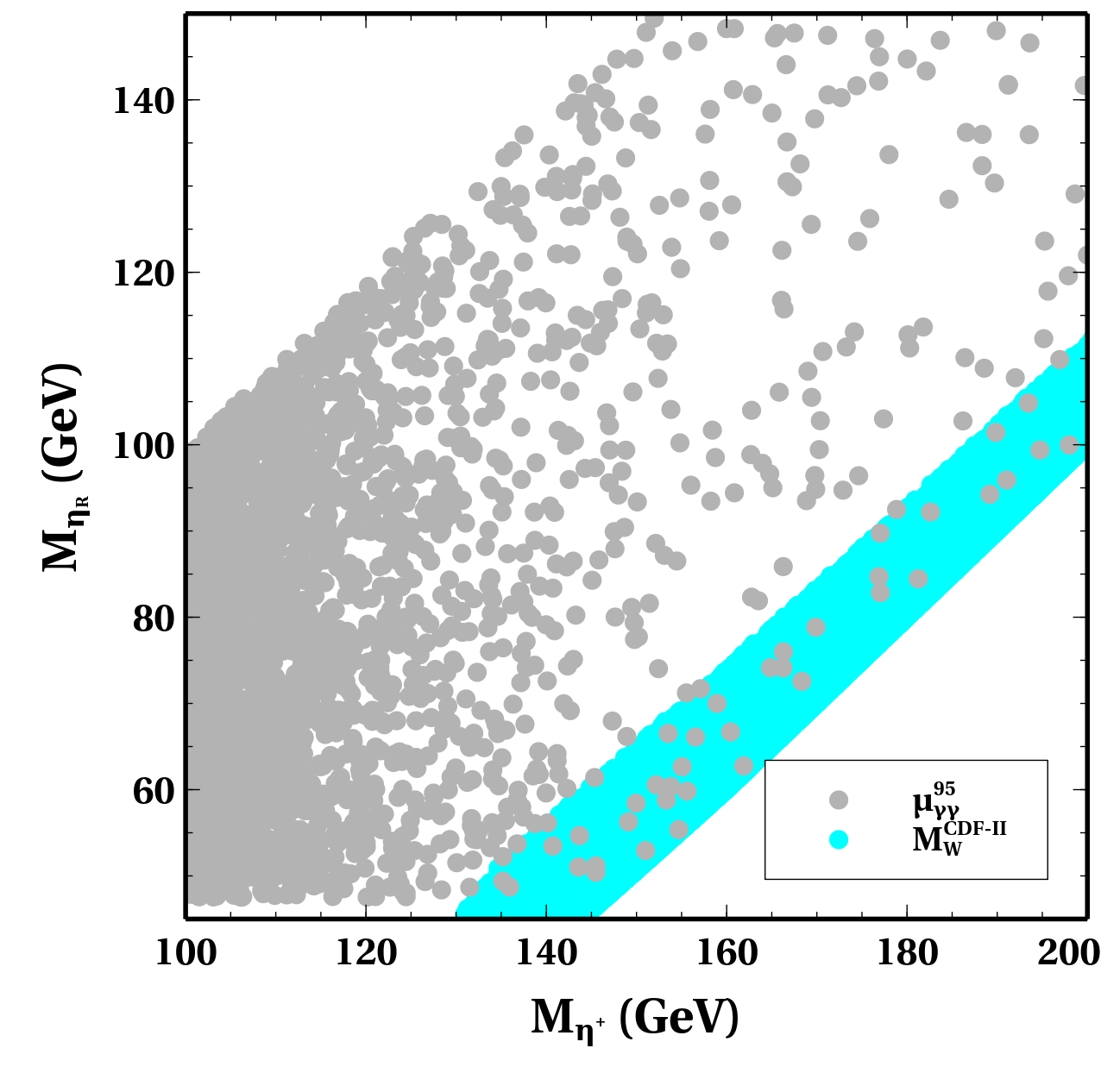
Figure 1: Parameter space satisfying CDF-II $W$-mass anomaly, 95 GeV excess in the plane of $M_{\eta_{R}}-M_{\eta^{+}}$ with one generation of $\eta$.

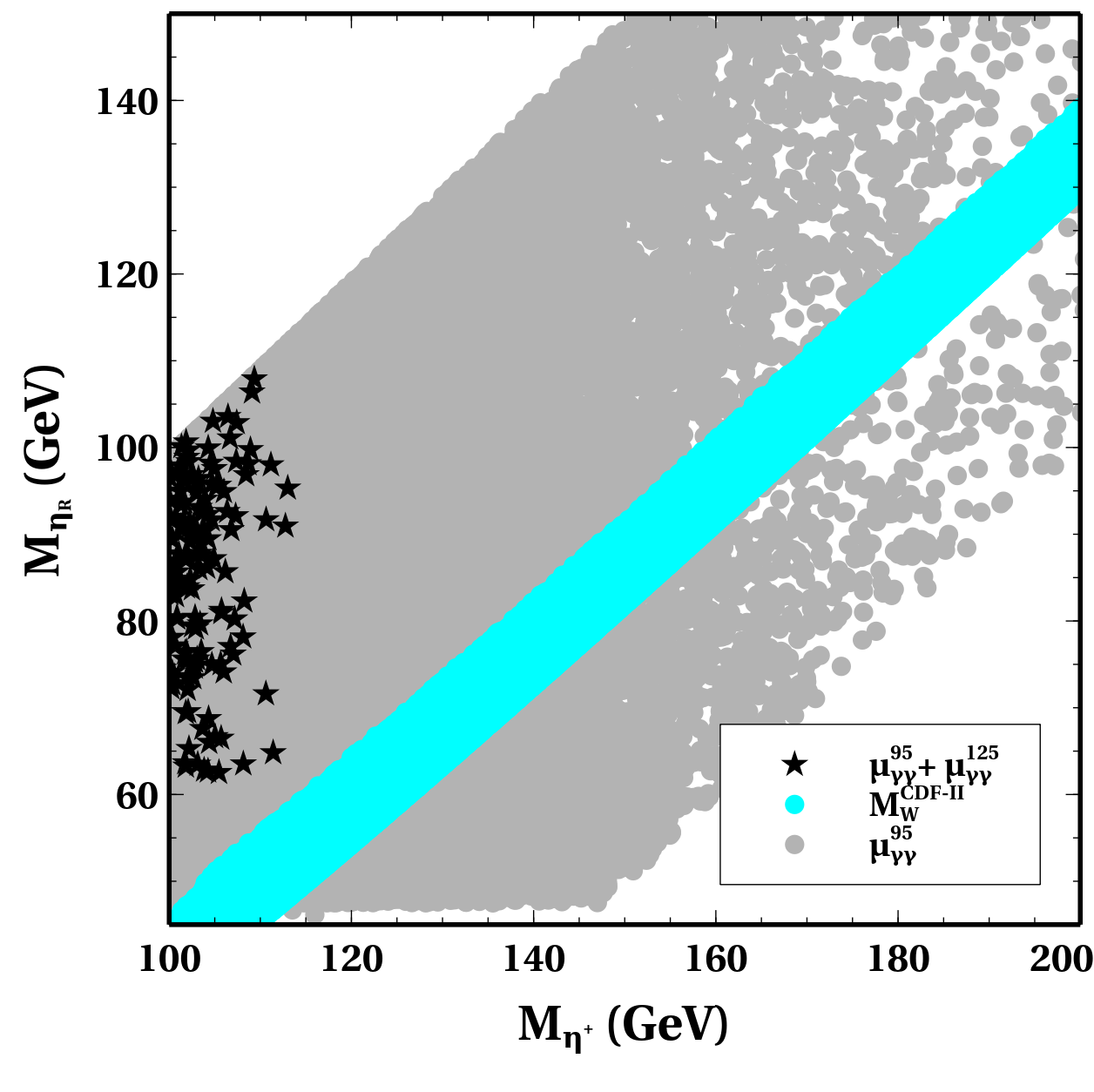
Figure 2: Parameter space satisfying CDF-II $W$-mass anomaly, 95 GeV excess in the plane of $M_{\eta_{R}}-M_{\eta^{+}}$ with two generations of $\eta$.

For the numerical scan, we consider the couplings $\lambda_{3}$, $\lambda_{5}$, $\lambda_{\eta\Phi_{1}}$, $\lambda_{\eta\Phi_{2}}$, the charged scalar mass $M_{\eta^{+}}$, and the CP-even scalar mass $M_{\eta_{R}}$ as free parameters and determine $M_{\eta_{I}}$ and $\lambda_{4}$ using Eq. (B), Eq. (B), and Eq. (78). These parameters are randomly varied within the following ranges: $M_{\eta_{R}}\in[45,150]$ GeV, $\lambda_{5}\in[10^{-8},10^{-2}]$, $\lambda_{3}\in[1,\sqrt{4\pi}]$, $M_{\eta^{+}}=M_{\eta_{R}}+[1,100]$ GeV, $\lambda_{\eta\Phi_{1}}\in[0.01,4\pi]$, $\lambda_{\eta\Phi_{2}}\in[0.01,4\pi]$. The scalar mixing angles are varied within the range: $\sin\theta_{12}\in[0.1,0.7]$, $\sin\theta_{23}\in[0.1,0.7]$, and $\sin\theta_{13}\in[0.001,0.01]$. Concerning the RHN mixing angles, two of them, $\beta_{13}=0$ and $\beta_{23}=\pi/4$, are uniquely determined due to the symmetry. The only mixing angle that is randomly varied is $\sin\beta_{12}\in[10^{-4},0.7]$. Further details on this can be found in Appendix A. Additionally, since the $H_{2}\eta^{+}\eta^{-}$ vertex depends on the VEV of $\Phi_{1}$, we randomly vary it as $v_{1}\in[20,60]$ GeV and determine $v_{2}$ using Eq. (13). Throughout the whole analysis, we have ensured that all the couplings adhere to the perturbative bounds. We also impose the LEP limits on the doublet scalar as $M_{\eta_{R}}+M_{\eta_{I}}>M_{Z}$ and a conservative limit on the charged scalar $M_{\eta^{+}}>100$ GeV.

In Fig. 1, we illustrate the parameter space that corresponds to the observed 95 GeV diphoton signal strength in the $M_{\eta_{R}}$ and $M_{\eta^{+}}$ plane, represented in grey. In the same plane, we depict the parameter space satisfying the W-mass anomaly in cyan. It is evident that, in this scenario, the mass difference between the charged and neutral components of the inert doublet falls within the range of $[80,100]$ GeV, ensuring the required $T$ and $S$ parameters capable of explaining the CDF W-mass anomaly. However, it is important to note that for the validation of this parameter space, its consistency with the measured SM Higgs signal strength in the diphoton channel should be verified. The measured value of this signal strength is $\mu^{\gamma\gamma}_{H_{\rm SM}}=1.1\pm 0.07$ Zyla et al. (2020) in the $1\sigma$ limit. This is essential because the same newly introduced BSM particles also influence the SM Higgs branching ratio to the diphoton channel. Upon incorporating this constraint into the analysis, it becomes evident that none of the points depicted in Fig. 1 align with the SM Higgs signal strength. In this case, the SM Higgs signal strength falls within the range of $[10^{-6},~{}0.45]$. This deviation arises from the distinctive nature of our gauged $U(1)_{L_{\mu}-L_{\tau}}$ scotogenic scenario compared to the usual scotogenic models augmented by $Z_{2}$-even singlet scalars. In models such as Escribano et al. (2023), which involve only one generation of $\eta$, the $Z_{2}$-even scalars decay into $\gamma\gamma$ via $\eta^{+}$ in the loop, in addition to the standard model channels. In contrast, in our gauged $U(1)_{L_{\mu}-L_{\tau}}$ scotogenic scenario, we have two additional decay modes for the scalars, namely, $H_{i}\rightarrow N_{1}N_{1}$ and $H_{i}\rightarrow Z_{\mu\tau}Z_{\mu\tau}$. Even if $H_{i}\rightarrow N_{1}N_{1}$ is tuned by suitable choices of Yukawa couplings, the latter can not be tuned arbitrarily due to tight constraints on $g_{\mu\tau},M_{Z_{\mu\tau}}$ from $(g-2)_{\mu}$ as we discuss later. The presence of these decay modes significantly reduces the SM Higgs branching for the diphoton channel, resulting in a signal strength much less than 1. Here, $H_{\rm SM}\rightarrow Z_{\mu\tau}Z_{\mu\tau}$ contribute dominantly in reducing the SM Higgs branching to $\gamma\gamma$.

To salvage the scenario, we introduce additional generations of $\eta$ to enhance the contribution to $H_{\text{SM}}\rightarrow\gamma\gamma$. This augmentation allows for the explanation of both the SM Higgs signal strength, the observed 95 GeV diphoton signal strength, and the W-mass anomaly. As depicted in Fig. 2, it becomes evident that with two generations of $\eta$, the mass of which we assume to be the same, it is possible to simultaneously account for the 95 GeV signal strength and SM Higgs signal strength, which is shown by the black star-shaped points in the figure. This constrains the charged scalar mass approximately in the range of $\sim[100,115]$ GeV. However, it is important to note that no common parameter space satisfies all three criteria simultaneously, including the W-mass anomaly. Nevertheless, it is worth highlighting that with two generations of the inert doublet, the mass splitting between the charged and neutral components of the inert doublet is reduced to $[50,70]$ GeV. Compared to Fig. 1, in Fig. 2, the W-mass region shifts upwards due to the decreased mass splitting. Clearly, if we can further decrease this mass splitting, we can get a common parameter space satisfying all three criteria. Introduction of an additional generation of inert scalar doublet makes this possible. The common parameter space satisfying the 95 GeV excess, SM Higgs signal strength, and W-mass anomaly simultaneously is presented in Fig. 3 depicted by the red colored points. In this scenario, the required mass splitting between $M_{\eta^{+}}$ and $M_{\eta_{R}}$ to explain the W-mass anomaly is approximately in the range of $[42,58]$ GeV. With three generations of $\eta$, the allowed mass range for $\eta^{+}$ based on the 95 GeV and SM Higgs diphoton signal strength is $[105,140]$ GeV, while $M_{\eta_{R}}$ is in the range $[62.5,90]$ GeV. For simplicity, we assume that the three doublets scalars are decoupled, meaning inter-generation mixings are absent.

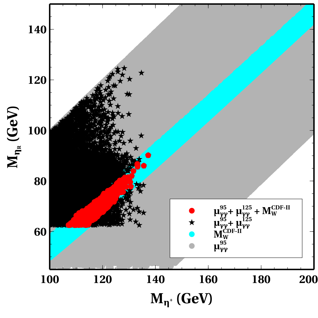
Figure 3: Parameter space satisfying CDF-II $W$-mass anomaly, 95 GeV excess and SM Higgs signal strength in the plane of $M_{\eta_{R}}-M_{\eta^{+}}$ with three generations of $\eta$.

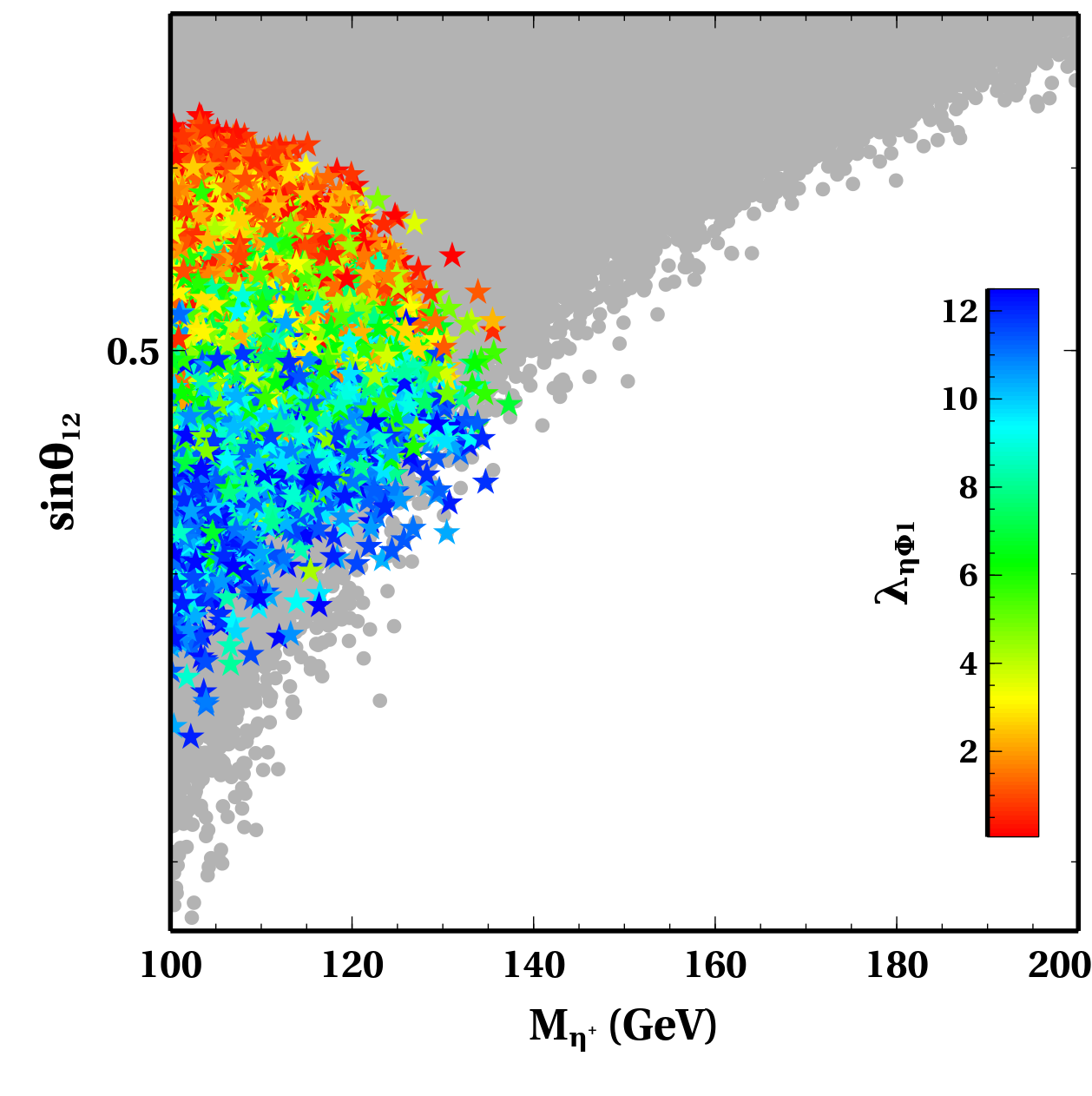
Figure 4: Parameter space satisfying 95 GeV excess and SM Higgs signal strength in the plane of $\sin\theta_{12}-M_{\eta^{+}}$ with three generations of $\eta$. Grey coloured points are consistent with 95 GeV excess and W-mass anomaly but can not satisfy SM Higgs signal strength.

We also illustrate the parameter space in the $\sin\theta_{12}-M_{\eta^{+}}$ plane in Fig. 4. The colored region in this plot satisfies both the 95 GeV scalar signal strength and the SM Higgs signal strength. The grey points depict the parameter space that aligns with the 95 GeV diphoton signal strength and W-mass anomaly but contradicts the SM Higgs diphoton signal strength. In this context, the scalar mixing angle $\sin\theta_{12}$ is confined within the range $[0.35,0.63]$. The correlation observed between the coupling $\lambda_{\eta\Phi_{1}}$ and mixing angle $\sin\theta_{12}$ arises from the increase in decay width for larger values of $\lambda_{\eta\Phi_{1}}$, facilitating the explanation of the signal strength with smaller mixing angles. Despite permitting the RHN mixing angle $\sin\beta_{12}$ to vary up to $0.7$, it is constrained to be within $0.1$ based on the 95 GeV excess and SM Higgs signal strength. This constraint emerges because larger values of $\sin{\beta_{12}}$ lead to prominence of the $H_{i}\rightarrow N_{1}N_{1}$ decay mode, resulting in a decrease in the corresponding diphoton branching and rendering it insufficient to explain the excess.

V Neutrino Mass

As previously discussed, the Majorana neutrino mass is induced at the one-loop level, involving the participation of particles from the dark sector in a manner akin to scotogenic model Tao (1996); Ma (2006). Due to the imposed symmetry that governs the interactions, it becomes evident from Eq. (1) that both the charged lepton mass matrix and the Dirac Yukawa matrix of neutrinos exhibit a diagonal structure. Consequently, the non-trivial neutrino mixing can be generated by the structure of the RHN mass matrix, which is generated by the scalar singlet fields. The charged lepton mass matrix, neutrino Dirac Yukawa matrix, and the right-handed neutrino mass matrix respectively, are given by

$$M_{\ell}=\frac{1}{\sqrt{2}}\begin{pmatrix}Y_{e}v&0&0\\ 0&Y_{\mu}v&0\\ 0&0&Y_{\tau}v\end{pmatrix},\,Y_{D}=\begin{pmatrix}Y_{De}&0&0\\ 0&Y_{D\mu}&0\\ 0&0&Y_{D\tau}\end{pmatrix},\,$$

$$M_{R}=\begin{pmatrix}M_{ee}&Y_{e\mu}v_{1}&Y_{e\tau}v_{1}\\ Y_{e\mu}v_{1}&Y_{\mu}v_{2}&M_{\mu\tau}\\ Y_{e\tau}v_{1}&M_{\mu\tau}&Y_{\tau}v_{2}\end{pmatrix}\,.$$ (31)

The neutrino mass arising at one-loop is given by: Ma (2006); Merle and Platscher (2015)

$$(M_{\nu})_{\alpha\beta}\ =\ \sum_{k}\frac{Y_{\alpha k}Y_{k\beta}M_{k}}{32\pi^{2}}\left[L_{k}(M^{2}_{\eta_{R}})-L_{k}(M^{2}_{\eta_{I}})\right]\,,$$ (32)

where $M_{k}$ represents the mass eigenvalue associated with the right-handed neutrino mass eigenstate $N_{k}$ running in the internal line, with the indices $\alpha$ and $\beta$ ranging from 1 to 3, covering the three neutrino generations. The Yukawa couplings $Y_{\alpha k}$ in the given neutrino mass formula are obtained from the Dirac Yukawa couplings in Lagrangian (1) by transitioning to the diagonal basis of right-handed neutrinos after spontaneous symmetry breaking. The loop function $L_{k}(m^{2})$ in neutrino mass formula (32) is defined as

$$L_{k}(m^{2})\ =\ \frac{m^{2}}{m^{2}-M^{2}_{k}}\>\text{ln}\frac{m^{2}}{M^{2}_{k}}\,.$$ (33)

It is noteworthy that the mass difference between the neutral scalar and pseudo-scalar components of $\eta$ ($m^{2}_{\eta_{R}}-m^{2}_{\eta_{I}}=\lambda_{5}v^{2}$) plays a pivotal role in generating a non-zero neutrino mass. For the analysis, the initial step involves diagonalizing $M_{R}$ and considering the physical basis of right-handed neutrinos $(N_{1},N_{2},N_{3})$ with appropriate interactions. Employing the Casas-Ibarra (CI) parametrization Casas and Ibarra (2001) extended to the radiative seesaw model Toma and Vicente (2014), we express the Yukawa coupling matrix that satisfies the neutrino oscillation data as follows:

$$Y_{\alpha k}\ =\ \left(UD_{\nu}^{1/2}R^{\dagger}\Lambda^{1/2}\right)_{\alpha k}\,,$$ (34)

In this expression, $R$ is an arbitrary complex orthogonal matrix satisfying $RR^{T}=\mathrm{I}$. The diagonal light neutrino mass matrix is denoted by $D_{\nu}=\textrm{diag}(m_{1},m_{2},m_{3})$, and the diagonal matrix $\Lambda$ has elements given by:

$$\Lambda_{k}\ =\ \frac{2\pi^{2}}{\lambda_{5}}\zeta_{k}\frac{2M_{k}}{v^{2}}\,,$$ (35)

$$\textrm{and}\quad\zeta_{k} \ =\ \left(\frac{M_{k}^{2}}{8(M_{\eta_{R}}^{2}-M_{\eta_{I}}^{2})}\left[L_{k}(M_{\eta_{R}}^{2})-L_{k}(M_{\eta_{I}}^{2})\right]\right)^{-1}\,.$$ (36)

VI Muon (g-2) Anomaly

The magnetic moment of the muon is expressed as:

$$\overrightarrow{\mu_{\mu}}=g_{\mu}\left(\frac{q}{2m}\right)\overrightarrow{S}\,,$$ (37)

where $g_{\mu}$ denotes the gyro-magnetic ratio, assuming a value of 2 for an elementary spin-$\frac{1}{2}$ particle with mass $m$ and charge $q$. At the tree level, conforming to the Dirac equation, it is theoretically exact at 2. However, within the framework of quantum field theory, minuscule corrections to this value emerge owing to the particle’s interactions with virtual particles and quantum effects. These corrections are parameterized as $a_{\mu}=(g_{\mu}-2)/2$. In our framework, the primary augmentation to the muon magnetic moment predominantly comes from the one-loop diagram facilitated by the $L_{\mu}-L_{\tau}$ gauge boson, denoted as $Z_{\mu\tau}$. The associated one-loop contribution is expressed as Brodsky and De Rafael (1968); Baek and Ko (2009):

$$\Delta a_{\mu}=\frac{\alpha_{\mu\tau}}{2\pi}\int^{1}_{0}dx\frac{2m^{2}_{\mu}x^{2}(1-x)}{x^{2}m^{2}_{\mu}+(1-x)M^{2}_{Z_{\mu\tau}}}$$ (38)

Here, $\alpha_{\mu\tau}$ is defined as $\alpha_{\mu\tau}=g^{2}_{\mu\tau}/(4\pi)$.

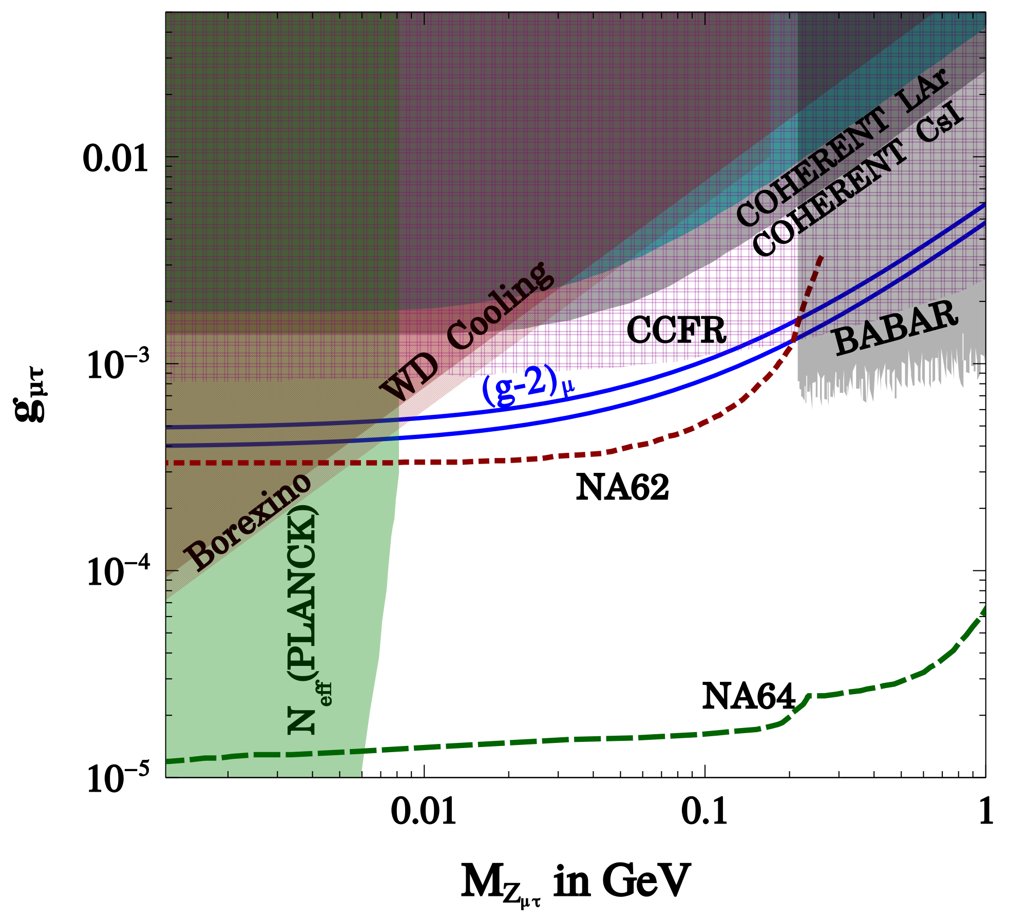
Figure 5: Parameter space satisfying correct $(g-2)_{\mu}$ in the plane of $g_{\mu\tau}-M_{Z_{\mu\tau}}$. See text for details of various constraints imposed on the parameter space.

In Fig. 5, we present the parameter space that satisfies the muon $g-2$ in the $g_{\mu\tau}$ - $M_{Z_{\mu\tau}}$ plane. This parameter space is constrained by various exclusion limits from different experiments, namely, CCFR Altmannshofer et al. (2014), COHERENT Akimov et al. (2017, 2021), BABAR Lees et al. (2016). The neutrino trident constraint from CCFR is shown by a magenta-colored mesh since some backgrounds have not been properly taken into account Krnjaic et al. (2020); Amaral et al. (2021). Exclusion zones from astrophysical bounds, specifically related to the cooling of white dwarfs (WD) Bauer et al. (2020); Kamada et al. (2018), are observed in the upper-left triangular region of Fig. 5. Additionally, constraints from Borexino Bellini et al. (2011), as discussed in  Gninenko and Gorbunov (2021), rule out a slightly larger portion compared to WD cooling constraints. Cosmological considerations of effective relativistic degrees of freedom Aghanim et al. (2018); Kamada et al. (2018); Ibe et al. (2020); Escudero et al. (2019) have effectively eliminated the possibility of very light $Z_{\mu\tau}$. This is due to the fact that delayed decay of light gauge bosons into SM leptons after the standard neutrino decoupling temperature leads to an increase in effective relativistic degrees of freedom $N_{\rm eff}$, tightly constrained by cosmic microwave background observations. Dashed lines in the figure represent the future sensitivities of NA62 Krnjaic et al. (2020) and NA64 Gninenko et al. (2015); Gninenko and Krasnikov (2018) experiments. Clearly, a small region of parameter space offering a potential explanation for the muon $(g-2)$ and allowed from other experimental constraints remains verifiable in near future. Similar observations have been made in previous studies on the minimal $L_{\mu}-L_{\tau}$ model Borah et al. (2020); Zu et al. (2021); Amaral et al. (2021); Zhou (2021); Borah et al. (2021a, c); Holst et al. (2021); Singirala et al. (2021); Hapitas et al. (2021).

It should also be noted that in the scotogenic version of the $L_{\mu}-L_{\tau}$ model, an extra one-loop diagram can also contribute to the anomalous magnetic moment. This diagram involves the charged component of the scalar doublet, denoted as $\eta^{+}$, and the right-handed neutrino $N_{k}$ in the loop, as shown in Fig. 6. However, this diagram can yield negative contributions to the anomalous magnetic moments of the muon.

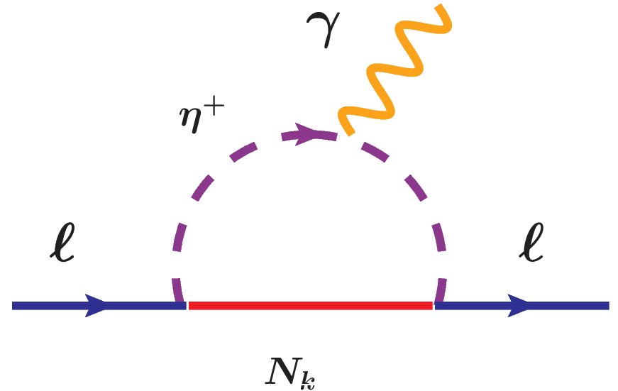
Figure 6: Contribution to $(g-2)_{\mu}$ from $\eta^{+}$ and RHN in the loop.

This contribution from the charged scalar loop is given by Queiroz and Shepherd (2014); Jana et al. (2020)

$$\Delta a_{\mu}=\sum_{k}-\frac{m^{2}_{\mu}}{8\pi^{2}M^{2}_{\eta^{+}}}\lvert Y_{\mu k}\rvert^{2}f(M^{2}_{k}/M^{2}_{\eta^{+}})$$ (39)

where

$$f(x)=\frac{1-6x+3x^{2}+2x^{3}-6x^{2}\log{x}}{12(1-x)^{4}}$$ (40)

Incorporating this contribution into the overall $(g-2)_{\mu}$ emphasizes the necessity for the positive contribution from the vector boson loop, surpassing that from the charged scalar loop. This guarantees the overall positivity of the muon $(g-2)$ in line with experimental observations. As illustrated in Fig. 5, there remains a parameter space not constrained by experiments, allowing for a larger positive contribution to the muon $(g-2)$ from the vector boson loop. Therefore, even if the $\eta^{+}$ loop contributes negatively to the muon $(g-2)$, the observed muon $(g-2)$ can be explained by a combination of positive and negative contributions within the scotogenic $L_{\mu}-L_{\tau}$ model.

VI.1 Lepton flavour violation

Charged lepton flavor-violating (CLFV) decays have been considered to be promising probes of physics beyond the SM. If we consider only the SM particle content with massive neutrinos, these processes occur only at the one-loop level and are significantly suppressed due to the tiny masses of neutrinos, keeping them well beyond the reach of current and future experimental sensitivities Baldini et al. (2016). Consequently, any future detection of CLFV decays, such as $\mu\rightarrow e\gamma$, would serve as a distinctive indicator of physics beyond the SM. Within our model, a new one-loop contribution to CLFV arises from the charged component of $\eta$ and right-handed neutrinos in the loop, as illustrated in Fig. 6. The branching ratio for the process $\mu\rightarrow e\gamma$ can be computed as Lavoura (2003); Toma and Vicente (2014)

$${\rm Br}(\mu\rightarrow e\gamma)=\frac{3(4\pi)^{3}\alpha}{4G^{2}_{F}}(\lvert A_{e\mu}^{M}\rvert^{2}+\lvert A_{e\mu}^{E}\rvert^{2}){\rm Br}(\mu\rightarrow e\nu_{\mu}\overline{\nu_{e}}).$$ (41)

Here, $A_{e\mu}^{M,E}$ are the dipole form factors that are provided in Appendix D. The most recent constraint from the MEG collaboration is $\text{Br}(\mu\rightarrow e\gamma)<4.2\times 10^{-13}$ at a $90\%$ CL Baldini et al. (2016). We use this bound to constrain our parameter space, consistent with the desired phenomenology mentioned above, before proceeding with the DM analysis.

VII Dark matter phenomenology

The model we consider here has two potential DM candidates, given that both the inert doublet scalar and the right-handed singlet fermions have odd parity under the $Z_{2}$ symmetry, ensuring their stability. Since the doublet scalar $\eta$ plays a pivotal role in addressing the $W$-mass anomaly and explaining the 95 GeV excess, the scalar mass spectrum, and couplings are already tightly constrained by these requirements. Consequently, our focus shifts to the study of the fermionic DM phenomenology within this framework.

In our scenario, the lightest among all the odd-sector particles, denoted as $N_{1}$, assumes the role of dark matter. The thermal freeze-out mechanism is employed to realize the dark matter relic. Since $N_{1}$ is a singlet under the SM gauge symmetry, its production mechanism is intricately tied to its Yukawa couplings with scalars and fermions of the model as well as the $U(1)_{L_{\mu}-L_{\tau}}$ gauge couplings. While $U(1)_{L_{\mu}-L_{\tau}}$ gauge coupling is restricted to a tiny window from $(g-2)_{\mu}$ criteria, a large Yukawa coupling with SM leptons can be achieved through Casas-Ibarra parametrization by tuning $\lambda_{5}$ to smaller values. We have used $\lambda_{5}$ in the range $\lambda_{5}\in[3\times 10^{-8},10^{-5}]$ which gives the Yukawas in the range $Y_{\alpha k}\in[10^{-4},10^{-2}$]. In this WIMP realization of fermion singlet DM, the processes contributing to the relic density via thermal freeze-out fall into three categories: (a) DM particles annihilate to SM particles or $Z_{\mu\tau}$ through the t or u-channel processes; (b) DM particles annihilate into SM particles and $Z_{\mu\tau}$ through s-channel scalar mediation; (c) the coannihilations among the DM particle and the next lightest dark sector particles, as well as the annihilations of the coannihilation partners into SM sectors and $Z_{\mu\tau}$. The relic density of DM has been computed using micrOMEGAS Belanger et al. (2014), which takes into account all relevant annihilation and coannihilation processes.

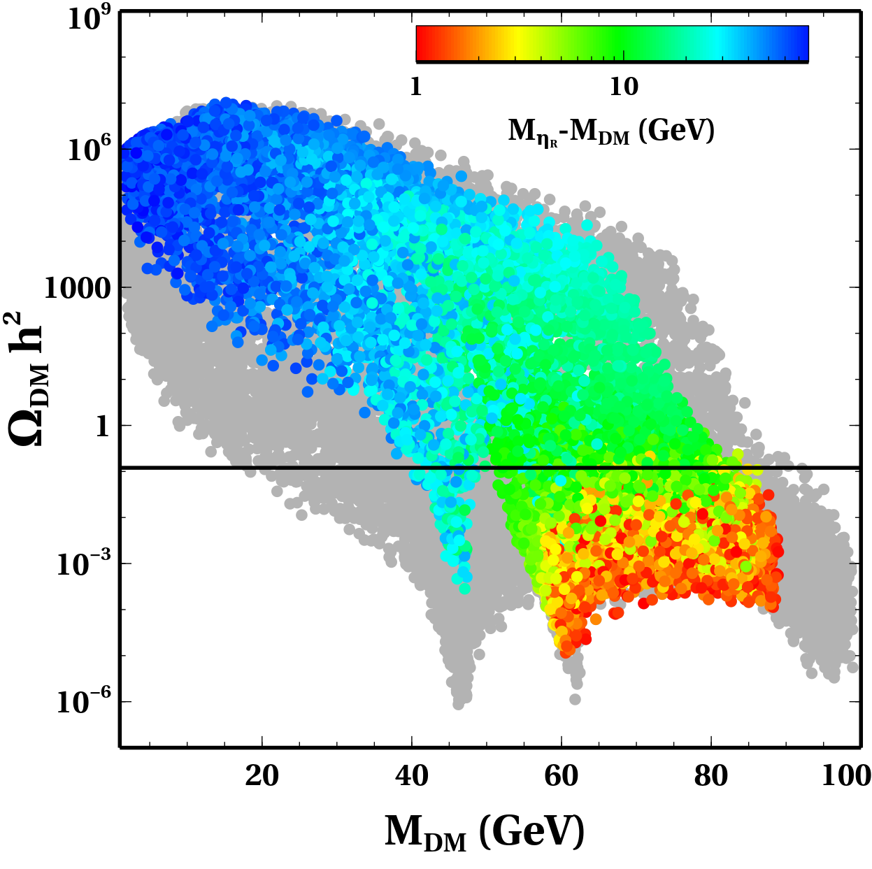
Figure 7: DM relic density as a function of DM mass.

We have shown the variation of DM relic density as a function of DM mass in Fig. 7. For the scan, the Yukawa couplings are calculated using the Cassa-Ibarra parametrization, given in Eq. (34). The right handed neutrinos are varied in the range : $M_{N_{1}}\equiv M_{\rm DM}\in[1,250]$ GeV, $M_{N_{2}}=M_{N_{3}}$=$M_{N_{1}}+100$ GeV while all other parameters are varied as discussed in section IV. The grey region in Fig. 7 is excluded by imposing the constraints from W-mass anomaly, 95 GeV signal strength, and SM Higgs signal strength, as discussed earlier. The color coding shows the mass splitting between the DM and the next to lightest stable particle (NLSP), $\eta_{R}$. This mass splitting plays an important role in determining the processes which are involved in the relic generation. When the mass splitting is large, the coannihilations are negligible, and the scalar-mediated annihilation channels dominate. The sharp dips around $47.5$ GeV and $62.5$ GeV are due to the scalar resonances corresponding to 95 GeV scalar $H_{2}$ and SM Higgs $H_{1}$. When that mass splitting between DM and NLSP decreases, the contributions of co-annihilation processes also become significant in addition to the annihilation processes, and consequently, the relic decreases, as seen from Fig. 7. Clearly, we can see that correct relic densityAghanim et al. (2020) can be achieved for DM mass in the range $M_{\rm DM}\in[40,85]$ GeV.

Since DM is of WIMP type, we have the possibility of probing it at direct detection experiments. Here, the DM-nucleon scattering is possible via scalar and vector boson mediated interactions, as shown in Fig. 8.

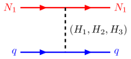
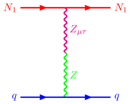
Figure 8: DM-nucleon scattering mediated by the scalars (top) and vector bosons (bottom).

The spin-independent (SI) DM-nucleon cross-section via scalar mediation is given as Ellis et al. (2008)

$$\sigma^{\rm SI}_{\rm scalar}=\frac{\mu_{r}^{2}}{\pi A^{2}}[\mathcal{M}]^{2}$$ (42)

where $\mu_{r}=\frac{M_{\rm DM}m_{n}}{M_{\rm DM}+m_{n}}$ is the reduced mass, $m_{n}$ is the nucleon (proton or neutron) mass. $\mathcal{M}$ is the amplitude corresponding to the scalar mediated diagram shown in Fig. 8. This amplitude is given as,

$$\mathcal{M}=\mathcal{Z}f_{p}+(A-\mathcal{Z})f_{n}$$ (43)

where $A$ is the mass number of target nucleus, $\mathcal{Z}$ is the atomic number of target nucleus. The $f_{p}$, and $f_{n}$ are the interaction strengths of proton and neutron with DM, respectively, and are given as,

$$f^{i}_{p,n}=\sum_{q=u,d,s}f_{T_{q}}^{p,n}\alpha^{i}_{q}\frac{m_{p,n}}{m_{q}}+\frac{2}{27}f_{T_{G}}^{p,n}\sum_{q=c,t,b}\alpha^{i}_{q}\frac{m_{p,n}}{m_{q}}$$ (44)

where,

$$\alpha^{i}_{q}=Y_{H_{i}}\times\frac{m_{q}}{v}\times\bigg{(}\frac{1}{m^{2}_{H_{i}}}\bigg{)}$$ (45)

Here the values of $f_{T_{q}}^{p,n}$, $f_{T_{G}}^{p,n}$ can be found in Ellis et al. (2000). In the above equation, $Y_{H_{i}}$ are the effective couplings between DM and the scalars ($H_{1}$, $H_{2}$, and $H_{3}$) and are given as,

$$Y_{H_{1}} =\sin{\beta_{12}}\cos{\beta_{12}}(-c_{12}s_{12}s_{23}-s_{23}c_{23})Y_{e\mu}+$$ (46)

$$\frac{1}{\sqrt{2}}\sin^{2}{\beta_{12}}(s_{12}s_{23}-c_{12}s_{13}c_{23})Y_{\mu}$$

$$Y_{H_{2}} =\sin{\beta_{12}}\cos{\beta_{12}}(-s_{12}s_{13}s_{23}+c_{12}c_{23})Y_{e\mu}+$$ (47)

$$\frac{1}{\sqrt{2}}\sin^{2}{\beta_{12}}(-c_{12}s_{23}-s_{12}s_{13}c_{23})Y_{\mu}$$

$$Y_{H_{3}} =\sin{\beta_{12}}\cos{\beta_{12}}(c_{13}s_{23})Y_{e\mu}+$$ (48)

$$\frac{1}{\sqrt{2}}\sin^{2}{\beta_{12}}(c_{13}c_{23})Y_{\mu}$$

where $s_{ij}$ and $c_{ij}$ are the scalar mixing angles and $\beta_{12}$ is the RHN mixing angle as discussed in Section IV and Appendix A respectively. The expressions for $Y_{e\mu}$ and $Y_{\mu}$ can be found in Appendix A.

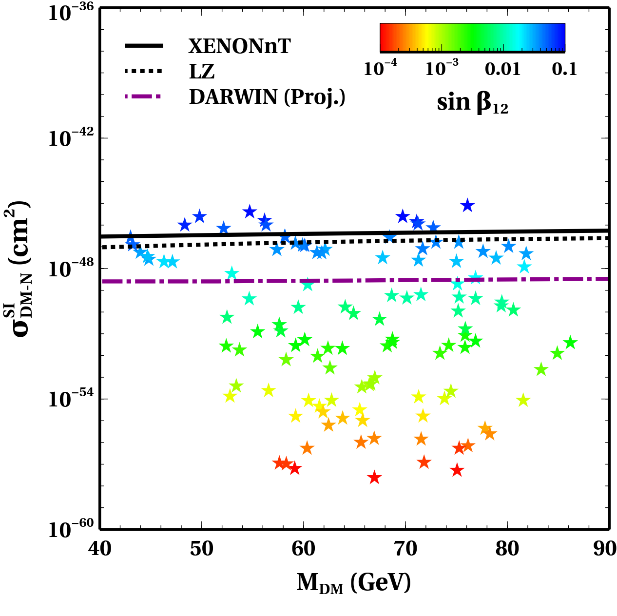
Figure 9: Spin-independent direct detection cross-section as a function of DM mass for the points satisfying correct relic density.

In addition to the scalar mediation process responsible for dark matter (DM)-nucleon scattering, a vector portal interaction can also occur due to the kinetic mixing between the $Z_{\mu\tau}$ and $Z$ bosons. The corresponding diagram is depicted in the lower panel of Fig. 8. Due to the nature of gauge coupling of DM, the scattering cross-section is either velocity-suppressed or spin-dependent, both of which lead to weak constraints. The spin-independent cross-section for the vector boson-mediated process is expressed as Chao (2019):

$$\sigma^{\rm SI}_{\rm vector}=\frac{2\mu^{2}_{r}}{\pi M^{4}_{Z_{\mu\tau}}}\sin^{4}{\beta_{12}}~{}g^{2}g^{2}_{\mu\tau}\epsilon^{2}v_{{}_{\rm DM}}^{2}$$ (49)

Here, $v_{{}_{\rm DM}}$ represents the velocity of the dark matter. It is important to note that, in gauged $L_{\mu}-L_{\tau}$ setup, the kinetic mixing parameter $\epsilon$ can not be tuned arbitrarily as it is induced at one-loop with particles charged under both $U(1)_{Y}$ and $U(1)_{L_{\mu}-L_{\tau}}$. The one-loop kinetic mixing is given by

$$|\epsilon_{\mu\tau}|\simeq\frac{gg_{\mu\tau}}{16\pi^{2}}\log\left(\frac{m_{\mu}}{m_{\tau}}\right)\simeq\frac{g_{\mu\tau}}{70}$$ (50)

Furthermore, spin-dependent DM-nucleon scattering can occur via vector boson mediation, with the cross-section given by

$$\sigma^{\rm SD}=\frac{4\mu^{2}_{r}}{\pi M^{4}_{Z_{\mu\tau}}}\sin^{4}{\beta_{12}}~{}g^{2}g^{2}_{\mu\tau}\epsilon^{2}\bigg{(}\sum_{q}\Delta^{N}_{q}\bigg{)}^{2}J_{N}(J_{N}+1).$$

Here, $J_{N}$ represents the angular momentum of the nucleon, and $\Delta^{N}_{q}$ denotes the spin fraction of quarks, as detailed in Agrawal et al. (2010). And our parameter space remains completely safe from the existing constraints Aalbers et al. (2023). So, for our analysis, we exclusively consider the spin-independent DM-nucleon scattering, which is rigorously constrained by terrestrial DM search experiments. We also note that the $\sigma^{\rm SI}_{\rm vector}$ always remains subdominant as compared to $\sigma^{\rm SI}_{\rm scalar}$ because of the velocity suppression.

We have shown SI direct detection cross-section as a function of DM mass in Fig. 9 where the color coding depicts the RHN mixing angle ($\beta_{12})$. Clearly, the existing experimental bounds from the XENON1T Aprile et al. (2018) and LZ Aalbers et al. (2023) put an upper bound on the mixing angle $\sin{\beta_{12}}<0.04$. However, future experiments like DARWIN Aalbers et al. (2016) has the potential to probe this mixing angle down to $\sin{\beta_{12}}=0.01$. Here, it is worth mentioning that, in addition to the tree-level DM-nucleon scattering process shown in Fig. 8, it can also arise at one-loop level with the doublet scalars in the loop as studied in Ibarra et al. (2016). However, because of loop suppression, it always remains subdominant as compared to the tree-level cross-section.

VIII Conclusion

We have studied the possibility of finding a common origin of three particle physics anomalies, namely, the muon $(g-2)$ anomaly, CDF-II W-mass anomaly, and CMS 95 GeV excess within the framework of scotogenic $L_{\mu}-L_{\tau}$ model which also explains the origin of light neutrino mass and dark matter in the Universe. While the lightest among the singlet right-handed neutrinos responsible for generating light neutrino mass plays the role of DM, the $L_{\mu}-L_{\tau}$ gauge boson explains the muon $(g-2)$ anomaly. The inert scalar doublet can lead to the required enhancement of W-boson mass via radiative corrections. While a neutral scalar formed out of the singlet scalars responsible for $L_{\mu}-L_{\tau}$ gauge symmetry breaking with a tiny admixture of the SM Higgs can play the role of the 95 GeV scalar, the required branching ratio for diphoton decay mode of this new light scalar together with that of the SM Higgs forces one to include two more inert Higgs doublets such that they can give rise to additional one-loop contributions to these decay widths without changing rest of the phenomenology. While these new scalar doublets do not play any additional role in our setup, they can be motivated from neutrino mass point of view if we have only one right-handed neutrino. The parameter space consistent with all the requirements remains verifiable at ongoing and near future experiments like dark matter direct detection, dark photon searches, charged lepton flavor violation, as well as colliders.

Appendix A RHN Masses and Mixing

The right-handed neutrino mass matrix in the flavor basis i.e. $(N_{e},N_{\mu},N_{\tau})^{T}$ is given by,

$$M_{R}=\left(\begin{array}[]{ccc}a&d&d\\ d&b&c\\ d&c&b\\ \end{array}\right)$$ (55)

where $a=M_{ee},~{}b=(Y_{\mu}=Y_{\tau})v_{2},~{}c=M_{\mu\tau},~{}d=(Y_{e\mu}=Y_{e\tau})v_{1}$. This is diagonalised by an unitary matrix, $U=U_{12}(\beta_{12}).U_{13}(\beta_{13}=0).U_{23}(\beta_{23}=\frac{\pi}{4})$ and given a diagonal mass matrix with definite masses, $M_{N_{1}}$, $M_{N_{2}}$, and $M_{N_{3}}$ with mass eigen states $N_{1}$, $N_{2}$, and $N_{3}$ respectively.
The mass basis is related to the flavor basis as,

$$\left(\begin{array}[]{c}N_{1}\\ N_{2}\\ N_{3}\\ \end{array}\right)=\left(\begin{array}[]{ccc}\cos\beta_{12}&\frac{\sin\beta_{12}}{\sqrt{2}}&\frac{\sin\beta_{12}}{\sqrt{2}}\\ -\sin\beta_{12}&\frac{\cos\beta_{12}}{\sqrt{2}}&\frac{\cos\beta_{12}}{\sqrt{2}}\\ 0&-\frac{1}{\sqrt{2}}&\frac{1}{\sqrt{2}}\\ \end{array}\right).\left(\begin{array}[]{c}N_{e}\\ N_{\mu}\\ N_{\tau}\\ \end{array}\right)$$ (66)

The mixing angle is given by,

$$\tan(2\beta_{12})=\frac{2\sqrt{2}d}{a-b-c}$$ (68)

The couplings and the mass parameters can be expressed in terms of the definite RHN masses and mixing angle as,

$$M_{ee}=\cos^{2}\beta_{12}M_{N_{1}}+\sin^{2}\beta_{12}M_{N_{2}}$$ (69)

$$Y_{\mu}=Y_{\tau} =\frac{1}{v_{2}}(\sin^{2}\beta_{12}\frac{M_{N_{1}}}{2}+\cos^{2}\beta_{12}\frac{M_{N_{2}}}{2}+\frac{M_{N_{3}}}{2})$$

$$M_{\mu\tau} =\frac{1}{v_{2}}(\sin^{2}\beta_{12}\frac{M_{N_{1}}}{2}+\cos^{2}\beta_{12}\frac{M_{N_{2}}}{2}-\frac{M_{N_{3}}}{2})$$ (71)

$$Y_{e\mu}=Y_{e\tau}=\frac{1}{v_{1}}\big{(}\frac{M_{N_{1}}}{\sqrt{2}}-\frac{M_{N_{2}}}{\sqrt{2}}\big{)}\cos\beta_{12}\sin\beta_{12}$$ (72)

Appendix B Physical masses of inert doublet scalar components

The $Z_{2}$-odd scalars can be written in component form as,

$$\eta=\left(\begin{array}[]{c}\eta^{+}\\ \frac{\eta_{R}+i\eta_{I}}{\sqrt{2}}\\ \end{array}\right)$$ (75)

The mass squared of the charged and neutral components are given as,

$$M_{\eta_{R}}^{2} =m_{\eta}^{2}+\frac{v^{2}}{2}(\lambda_{3}+\lambda_{4}+\lambda_{5})+\frac{v_{1}^{2}}{2}\lambda_{\eta\Phi_{1}}+\frac{v_{2}^{2}}{2}\lambda_{\eta\Phi_{2}}$$

$$M_{\eta_{I}}^{2} =m_{\eta}^{2}+\frac{v^{2}}{2}(\lambda_{3}+\lambda_{4}-\lambda_{5})+\frac{v_{1}^{2}}{2}\lambda_{\eta\Phi_{1}}+\frac{v_{2}^{2}}{2}\lambda_{\eta\Phi_{2}}$$

$$M_{\eta^{+}}^{2} =m_{\eta}^{2}+\frac{v^{2}}{2}\lambda_{3}+\frac{v_{1}^{2}}{2}\lambda_{\eta\Phi_{1}}+\frac{v_{2}^{2}}{2}\lambda_{\eta\Phi_{2}}$$ (78)

Appendix C Loop functions

The loop functions involved in the calculation of $\Gamma(h_{i}\to\gamma\gamma)$ are given by Djouadi (2008); Staub et al. (2016)

$$A_{0} =-[\tau-f(\tau)]/\tau^{2}\,,$$

$$A_{1/2} =2[\tau+(\tau-1)f(\tau)]/\tau^{2}\,,$$ (79)

$$A_{1} =-[2\tau^{2}+3\tau+3(2\tau-1)f(\tau)]/\tau^{2}\,,$$

where the function $f(\tau)$ is defined as

$$f(\tau)=\left\{\begin{array}[]{lc}\arcsin^{2}\sqrt{\tau};&\tau\leq 1\\ \\ -\frac{1}{4}\left[\log\frac{1+\sqrt{1-\tau^{-1}}}{1-\sqrt{1-\tau^{-1}}}-i\pi\right]^{2};&\tau>1\end{array}\right.$$ (83)

Appendix D CLFV

$$I^{(\pm)_{1}(\pm)_{2}}_{k}=\int d^{3}X\frac{x(y+(\pm)_{1}z\frac{m_{e}}{m_{\mu}}+(\pm)_{2}\frac{M_{k}}{m_{\mu}})}{-xym_{\mu}^{2}-xzm_{e}^{2}+(1-x)M_{\eta^{+}}^{2}+xM_{k}^{2}}$$

$$A_{e\mu}^{M}=\frac{-1}{(4\pi)^{2}}\sum_{k}(Y_{ek}^{*}Y_{\mu k}I^{++}_{k}+Y_{ek}^{*}Y_{\mu k}I^{+-}_{k})$$ (86)

$$A_{e\mu}^{E}=\frac{-i}{(4\pi)^{2}}\sum_{k}(-Y_{ek}^{*}Y_{\mu k}I^{-+}_{k}-Y_{ek}^{*}Y_{\mu k}I^{--}_{k})$$ (87)

References

- Abi et al. (2021) B. Abi et al. (Muon g-2), Phys. Rev. Lett. 126, 141801 (2021), eprint 2104.03281.
- Aguillard et al. (2023) D. P. Aguillard et al. (Muon g-2) (2023), eprint 2308.06230.
- Aoyama et al. (2020) T. Aoyama et al. (2020), eprint 2006.04822.
- Borsanyi et al. (2020) S. Borsanyi et al. (2020), eprint 2002.12347.
- Ignatov et al. (2023) F. V. Ignatov et al. (CMD-3) (2023), eprint 2302.08834.
- Jegerlehner and Nyffeler (2009) F. Jegerlehner and A. Nyffeler, Phys. Rept. 477, 1 (2009), eprint 0902.3360.
- Lindner et al. (2018) M. Lindner, M. Platscher, and F. S. Queiroz, Phys. Rept. 731, 1 (2018), eprint 1610.06587.
- Athron et al. (2021) P. Athron, C. Balázs, D. H. Jacob, W. Kotlarski, D. Stöckinger, and H. Stöckinger-Kim (2021), eprint 2104.03691.
- Sirunyan et al. (2019) A. M. Sirunyan et al. (CMS), Phys. Lett. B 793, 320 (2019), eprint 1811.08459.
- Tumasyan et al. (2023) A. Tumasyan et al. (CMS), JHEP 07, 073 (2023), eprint 2208.02717.
- CMS (2023) (2023).
- Barate et al. (2003) R. Barate et al. (LEP Working Group for Higgs boson searches, ALEPH, DELPHI, L3, OPAL), Phys. Lett. B 565, 61 (2003), eprint hep-ex/0306033.
- Cao et al. (2017) J. Cao, X. Guo, Y. He, P. Wu, and Y. Zhang, Phys. Rev. D 95, 116001 (2017), eprint 1612.08522.
- Haisch and Malinauskas (2018) U. Haisch and A. Malinauskas, JHEP 03, 135 (2018), eprint 1712.06599.
- Fox and Weiner (2018) P. J. Fox and N. Weiner, JHEP 08, 025 (2018), eprint 1710.07649.
- Liu et al. (2018) D. Liu, J. Liu, C. E. M. Wagner, and X.-P. Wang, JHEP 06, 150 (2018), eprint 1805.01476.
- Biekötter et al. (2020) T. Biekötter, M. Chakraborti, and S. Heinemeyer, Eur. Phys. J. C 80, 2 (2020), eprint 1903.11661.
- Cline and Toma (2019) J. M. Cline and T. Toma, Phys. Rev. D 100, 035023 (2019), eprint 1906.02175.
- Choi et al. (2019) K. Choi, S. H. Im, K. S. Jeong, and C. B. Park, Eur. Phys. J. C 79, 956 (2019), eprint 1906.03389.
- Kundu et al. (2020) A. Kundu, S. Maharana, and P. Mondal, Nucl. Phys. B 955, 115057 (2020), eprint 1907.12808.
- Cao et al. (2020) J. Cao, X. Jia, Y. Yue, H. Zhou, and P. Zhu, Phys. Rev. D 101, 055008 (2020), eprint 1908.07206.
- Biekötter et al. (2021) T. Biekötter, M. Chakraborti, and S. Heinemeyer, Int. J. Mod. Phys. A 36, 2142018 (2021), eprint 2003.05422.
- Abdelalim et al. (2022) A. A. Abdelalim, B. Das, S. Khalil, and S. Moretti, Nucl. Phys. B 985, 116013 (2022), eprint 2012.04952.
- Heinemeyer et al. (2022) S. Heinemeyer, C. Li, F. Lika, G. Moortgat-Pick, and S. Paasch, Phys. Rev. D 106, 075003 (2022), eprint 2112.11958.
- Biekötter et al. (2022) T. Biekötter, S. Heinemeyer, and G. Weiglein, JHEP 08, 201 (2022), eprint 2203.13180.
- Iguro et al. (2022) S. Iguro, T. Kitahara, and Y. Omura, Eur. Phys. J. C 82, 1053 (2022), eprint 2205.03187.
- Biekötter et al. (2023a) T. Biekötter, S. Heinemeyer, and G. Weiglein (2023a), eprint 2303.12018.
- Azevedo et al. (2023) D. Azevedo, T. Biekötter, and P. M. Ferreira (2023), eprint 2305.19716.
- Biekötter et al. (2023b) T. Biekötter, S. Heinemeyer, and G. Weiglein (2023b), eprint 2306.03889.
- Escribano et al. (2023) P. Escribano, V. M. Lozanoa, and A. Vicente (2023), eprint 2306.03735.
- Belyaev et al. (2023) A. Belyaev, R. Benbrik, M. Boukidi, M. Chakraborti, S. Moretti, and S. Semlali (2023), eprint 2306.09029.
- Aguilar-Saavedra et al. (2023) J. A. Aguilar-Saavedra, H. B. Câmara, F. R. Joaquim, and J. F. Seabra (2023), eprint 2307.03768.
- Bhattacharya et al. (2023) S. Bhattacharya, G. Coloretti, A. Crivellin, S.-E. Dahbi, Y. Fang, M. Kumar, and B. Mellado (2023), eprint 2306.17209.
- Ashanujjaman et al. (2023) S. Ashanujjaman, S. Banik, G. Coloretti, A. Crivellin, B. Mellado, and A.-T. Mulaudzi (2023), eprint 2306.15722.
- Aaltonen et al. (2022) T. Aaltonen et al. (CDF), Science 376, 170 (2022).
- He et al. (1991a) X. He, G. C. Joshi, H. Lew, and R. Volkas, Phys. Rev. D 43, 22 (1991a).
- He et al. (1991b) X.-G. He, G. C. Joshi, H. Lew, and R. R. Volkas, Phys. Rev. D 44, 2118 (1991b).
- Foot (1991) R. Foot, Mod. Phys. Lett. A 6, 527 (1991).
- Patra et al. (2017) S. Patra, S. Rao, N. Sahoo, and N. Sahu, Nucl. Phys. B 917, 317 (2017), eprint 1607.04046.
- Borah et al. (2020) D. Borah, S. Mahapatra, D. Nanda, and N. Sahu (2020), eprint 2007.10754.
- Borah et al. (2021a) D. Borah, M. Dutta, S. Mahapatra, and N. Sahu (2021a), eprint 2104.05656.
- Tao (1996) Z.-j. Tao, Phys. Rev. D 54, 5693 (1996), eprint hep-ph/9603309.
- Ma (2006) E. Ma, Phys. Rev. D73, 077301 (2006), eprint hep-ph/0601225.
- Baek (2016) S. Baek, Phys. Lett. B 756, 1 (2016), eprint 1510.02168.
- Borah et al. (2021b) D. Borah, M. Dutta, S. Mahapatra, and N. Sahu (2021b), eprint 2109.02699.
- Escribano et al. (2020) P. Escribano, M. Reig, and A. Vicente, JHEP 07, 097 (2020), eprint 2004.05172.
- Zyla et al. (2020) P. A. Zyla et al. (Particle Data Group), PTEP 2020, 083C01 (2020).
- Hollik (1990) W. F. L. Hollik, Fortsch. Phys. 38, 165 (1990).
- Nagashima (2010) Y. Nagashima, Elementary particle physics: Foundations of the standard model, volume 2 (Wiley-VCH, Weinheim, 2010), ISBN 978-3-527-40966-2.
- Borah et al. (2022a) D. Borah, S. Mahapatra, and N. Sahu, Phys. Lett. B 831, 137196 (2022a), eprint 2204.09671.
- Babu et al. (2022) K. S. Babu, S. Jana, and V. P. K., Phys. Rev. Lett. 129, 121803 (2022), eprint 2204.05303.
- Grimus et al. (2008) W. Grimus, L. Lavoura, O. M. Ogreid, and P. Osland, Nucl. Phys. B 801, 81 (2008), eprint 0802.4353.
- Borah et al. (2022b) D. Borah, S. Mahapatra, D. Nanda, and N. Sahu, Phys. Lett. B 833, 137297 (2022b), eprint 2204.08266.
- Djouadi (2008) A. Djouadi, Phys. Rept. 457, 1 (2008), eprint hep-ph/0503172.
- Merle and Platscher (2015) A. Merle and M. Platscher, JHEP 11, 148 (2015), eprint 1507.06314.
- Casas and Ibarra (2001) J. A. Casas and A. Ibarra, Nucl. Phys. B618, 171 (2001), eprint hep-ph/0103065.
- Toma and Vicente (2014) T. Toma and A. Vicente, JHEP 01, 160 (2014), eprint 1312.2840.
- Brodsky and De Rafael (1968) S. J. Brodsky and E. De Rafael, Phys. Rev. 168, 1620 (1968).
- Baek and Ko (2009) S. Baek and P. Ko, JCAP 10, 011 (2009), eprint 0811.1646.
- Altmannshofer et al. (2014) W. Altmannshofer, S. Gori, M. Pospelov, and I. Yavin, Phys. Rev. Lett. 113, 091801 (2014), eprint 1406.2332.
- Akimov et al. (2017) D. Akimov et al. (COHERENT), Science 357, 1123 (2017), eprint 1708.01294.
- Akimov et al. (2021) D. Akimov et al. (COHERENT), Phys. Rev. Lett. 126, 012002 (2021), eprint 2003.10630.
- Lees et al. (2016) J. Lees et al. (BaBar), Phys. Rev. D 94, 011102 (2016), eprint 1606.03501.
- Krnjaic et al. (2020) G. Krnjaic, G. Marques-Tavares, D. Redigolo, and K. Tobioka, Phys. Rev. Lett. 124, 041802 (2020), eprint 1902.07715.
- Amaral et al. (2021) D. W. P. Amaral, D. G. Cerdeño, A. Cheek, and P. Foldenauer (2021), eprint 2104.03297.
- Bauer et al. (2020) M. Bauer, P. Foldenauer, and J. Jaeckel, JHEP 18, 094 (2020), eprint 1803.05466.
- Kamada et al. (2018) A. Kamada, K. Kaneta, K. Yanagi, and H.-B. Yu, JHEP 06, 117 (2018), eprint 1805.00651.
- Bellini et al. (2011) G. Bellini et al., Phys. Rev. Lett. 107, 141302 (2011), eprint 1104.1816.
- Gninenko and Gorbunov (2021) S. Gninenko and D. Gorbunov, Phys. Lett. B 823, 136739 (2021), eprint 2007.16098.
- Aghanim et al. (2018) N. Aghanim et al. (Planck) (2018), eprint 1807.06209.
- Ibe et al. (2020) M. Ibe, S. Kobayashi, Y. Nakayama, and S. Shirai, JHEP 04, 009 (2020), eprint 1912.12152.
- Escudero et al. (2019) M. Escudero, D. Hooper, G. Krnjaic, and M. Pierre, JHEP 03, 071 (2019), eprint 1901.02010.
- Gninenko et al. (2015) S. Gninenko, N. Krasnikov, and V. Matveev, Phys. Rev. D 91, 095015 (2015), eprint 1412.1400.
- Gninenko and Krasnikov (2018) S. Gninenko and N. Krasnikov, Phys. Lett. B 783, 24 (2018), eprint 1801.10448.
- Zu et al. (2021) L. Zu, X. Pan, L. Feng, Q. Yuan, and Y.-Z. Fan (2021), eprint 2104.03340.
- Zhou (2021) S. Zhou (2021), eprint 2104.06858.
- Borah et al. (2021c) D. Borah, A. Dasgupta, and D. Mahanta (2021c), eprint 2106.14410.
- Holst et al. (2021) I. Holst, D. Hooper, and G. Krnjaic (2021), eprint 2107.09067.
- Singirala et al. (2021) S. Singirala, S. Sahoo, and R. Mohanta (2021), eprint 2106.03735.
- Hapitas et al. (2021) T. Hapitas, D. Tuckler, and Y. Zhang (2021), eprint 2108.12440.
- Queiroz and Shepherd (2014) F. S. Queiroz and W. Shepherd, Phys. Rev. D 89, 095024 (2014), eprint 1403.2309.
- Jana et al. (2020) S. Jana, P. K. Vishnu, W. Rodejohann, and S. Saad, Phys. Rev. D 102, 075003 (2020), eprint 2008.02377.
- Baldini et al. (2016) A. M. Baldini et al. (MEG), Eur. Phys. J. C76, 434 (2016), eprint 1605.05081.
- Lavoura (2003) L. Lavoura, Eur. Phys. J. C29, 191 (2003), eprint hep-ph/0302221.
- Belanger et al. (2014) G. Belanger, F. Boudjema, A. Pukhov, and A. Semenov, Comput. Phys. Commun. 185, 960 (2014), eprint 1305.0237.
- Aghanim et al. (2020) N. Aghanim et al. (Planck), Astron. Astrophys. 641, A6 (2020), [Erratum: Astron.Astrophys. 652, C4 (2021)], eprint 1807.06209.
- Ellis et al. (2008) J. R. Ellis, K. A. Olive, and C. Savage, Phys. Rev. D 77, 065026 (2008), eprint 0801.3656.
- Ellis et al. (2000) J. R. Ellis, A. Ferstl, and K. A. Olive, Phys. Lett. B481, 304 (2000), eprint hep-ph/0001005.
- Chao (2019) W. Chao, JHEP 11, 013 (2019), eprint 1904.09785.
- Agrawal et al. (2010) P. Agrawal, Z. Chacko, C. Kilic, and R. K. Mishra (2010), eprint 1003.1912.
- Aalbers et al. (2023) J. Aalbers et al. (LZ), Phys. Rev. Lett. 131, 041002 (2023), eprint 2207.03764.
- Aprile et al. (2018) E. Aprile et al. (2018), eprint 1805.12562.
- Aalbers et al. (2016) J. Aalbers et al. (DARWIN), JCAP 11, 017 (2016), eprint 1606.07001.
- Ibarra et al. (2016) A. Ibarra, C. E. Yaguna, and O. Zapata, Phys. Rev. D 93, 035012 (2016), eprint 1601.01163.
- Staub et al. (2016) F. Staub et al., Eur. Phys. J. C 76, 516 (2016), eprint 1602.05581.