Genuine multipartite entanglement without fully controllable measurements

Abstract

Standard procedures for entanglement detection assume that experimenters can exactly implement specific quantum measurements. Here, we depart from such idealizations and investigate, in both theory and experiment, the detection of genuine multipartite entanglement using measurements that are subject to small imperfections. We show how to correct well-known examples of multipartite entanglement witnesses to account for measurement imperfection, thereby excluding the possibility of false positives. We proceed with a tabletop four-partite photonic experiment and demonstrate first how a small amount of alignment error can undermine the conclusions drawn from uncorrected entanglement witnesses, and then the conclusions of the corrected data analysis. Furthermore, as our approach is tailored for a quantum device that is trusted but not flawlessly controlled, we show its advantages in terms of noise resilience as compared to device-independent models. Our work contributes to verifying quantum properties of multipartite systems when taking into account knowledge of imperfections in the verification devices.

I Introduction

Entanglement is generally regarded as the key resource in quantum information, allowing one to perform tasks that are classically impossible or to perform them at a faster rate. Deciding whether a given state is entangled is therefore a central challenge in quantum information [1, 2, 3]. The commonly used practice to certify entanglement of a given state is via the use of so-called entanglement witnesses. These are observables whose expectation value is bounded for separable states, but this bound can be surpassed by entangled states [4, 5, 6]. Such ideas also apply to the case of multiple parties, where one is often interested in certifying genuine multipartite entanglement (GME) via entanglement witnesses whose expectation value is bounded for biseparable states [7]. This trusted, or device-dependent, scenario of entanglement detection assumes perfect control over all the measurements. In other words, the actual measurements in the laboratory must correspond exactly to those intended for the verification protocol. This is an idealisation, and small experimental deviations are in fact known to cause significant possibilities of false positives [8, 9, 10].

A well-known way to circumvent the problem of imperfect measurements is to detect entanglement in a device-independent framework, i.e. without any assumptions on the quantum measurement devices. Hence, the measurements are treated as black-boxes and entanglement is detected via the violation of a Bell inequality [11, 12]. Similarly, this can be extended to detecting GME, by formulating stronger Bell-type inequalities, that cannot be violated by biseparable states  [11, 13]. In such a scenario the risk of false positives, owing to imperfect measurements, can be excluded. However, this comes both with the practical drawback that experiments become significantly more challenging and the fundamental drawback that many entangled states cannot be detected. While conceptually of great importance, it is arguably a far too generic model of the measurements when dealing with the common situation of trusted yet imperfectly controlled devices. Adopting a black-box picture to account for the lack of flawless control over non-malicious devices is in the spirit of killing a fly with an elephant gun.

Moving away from the two extremes, namely from having perfect control and from having no control at all, one may consider a framework for entanglement detection in which the experimenter controls the measurements, but only up to a given level of precision. The experimenter aims to perform a given measurement, but their lab measurement only nearly corresponds to it, see Fig 1 for an illustration. Recently, in the bipartite scenario, it has been shown how to correct some well-known standard entanglement witnesses to take small measurement imperfections into account [10]. In this work, we go further and study how imperfect devices can be accounted for when witnessing GME in multipartite systems. The relevance of taking small imperfections seriously has been theoretically shown through few-qubit entanglement witnesses in [9]. In fact, one might expect that the detrimental influence of measurement imperfections can accumulate over many separate subsystems, thus becoming an even more significant issue than in the bipartite case. We theoretically analyse this problem for several well-known witnesses of GME and show that this intuition does not always hold. In particular, for the seminal Greenberger-Horne-Zeilinger state, we analytically derive a tight GME witness for any number of qubits that takes measurement imperfection into account.

To showcase the relevance of taking small systematic imperfections into account for otherwise trusted devices, we carry out a series of experiments using a table-top four-photon source. We first implement a protocol in which entanglement between only three photons and small misalignment in a single measurement apparatus is used to generate a false positive of genuine four-party entanglement via the Mermin witness. Then, using our entanglement witness construction, which applies to arbitrary bounded errors, we show how to overcome the issue of imperfect control and faithfully demonstrate genuine four-photon GHZ-like entanglement. Furthermore, we apply the experimental data towards fidelity estimation for the prepared GHZ state. We show that the small imperfections in our measurements can require a significant revision of the conventional witness-based fidelity estimation. For our measurement errors, which never exceed a third of a percent and are often even lower, this can still imply a fidelity reduction by several percentage points. Finally, we study the relevance of our approach as compared to the more relaxed scenario of device-independent detection of GME. In the presence of dephasing noise on the source, we show that our approach, based on imperfect devices, indeed can detect GME at considerably higher noise rates than with well-known device-independent witnesses.

In summary, we provide an approach for efficient and reliable GME detection, that only requires an estimation of the precision of the performed measurements. It highlights the benefits of leveraging limited knowledge of measurement in detecting GME, as compared to a more powerful but less well-tailored device-independent approach.

II Imperfect qubit measurements

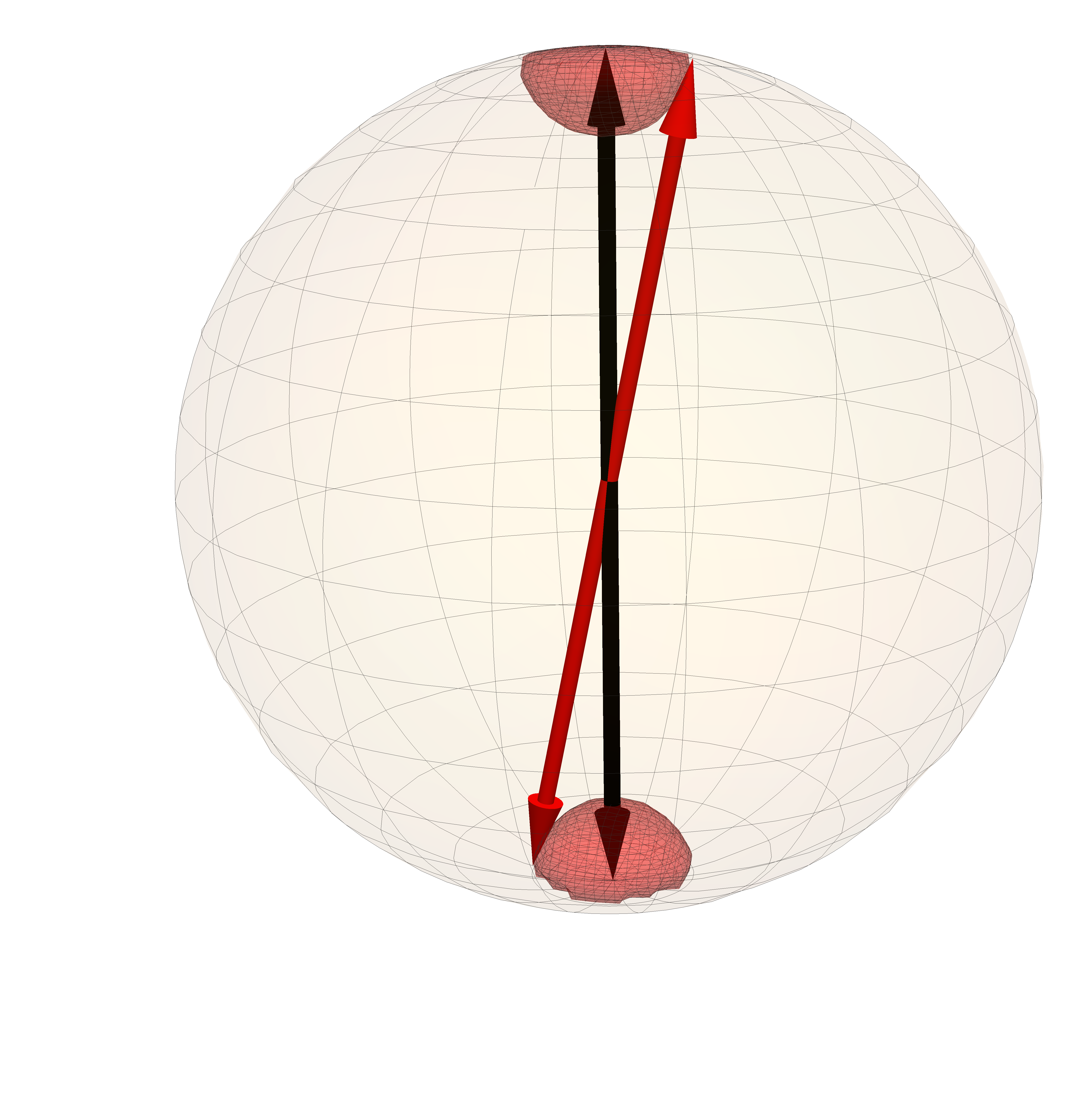
Figure 1: Imperfect measurement. The experimenter intends to perform a qubit measurement (black) but the lab measurement (red) is only a close approximation of it. The lab measurement is only assumed to be confined to a small region in the neigbourhood of the intended measurement.

When measuring an entanglement witness, an experimenter is asked to perform a collection of global product measurements, i.e. to measure each particle with respect to a given basis. For qubit systems, measuring a basis can be represented by the orthogonal projectors $P_{+}=\outerproduct{\vec{n}}{\vec{n}}$ and $P_{-}=\outerproduct{-\vec{n}}{-\vec{n}}$, where $\vec{n}\in\mathbb{R}^{3}$ is some unit Bloch vector. However, due to the lack of perfect control, the measurement implemented in the lab does not correspond exactly to the intended basis, but instead to some other measurement operators, $\tilde{P}_{+}$ and $\tilde{P}_{-}$, which closely approximate it, as visualized in Fig. 1. This lab measurement can be both noisy, meaning that its Bloch vector is not of unit length, and be misaligned, meaning that its Bloch vector has an orientation different from $\vec{n}$. Thus, it needs not to correspond to a basis measurement but instead to some POVM. In order to quantify how well the lab measurement approximates the intended measurement, it has been proposed to estimate their average fidelity [10],

$$\mathcal{F}_{\vec{n}}\equiv\frac{1}{2}\langle\vec{n}|\tilde{P}_{+}|\vec{n}\rangle+\frac{1}{2}\langle-\vec{n}|\tilde{P}_{-}|-\vec{n}\rangle.$$ (1)

While in principle any distance-like measure can be used for this purpose, this particular measure has the advantage that it can be readily estimated in the lab using elementary resources. The experimenter needs only to employ an auxiliary source and prepare the eigenstates of the intended measurement, which are then used to probe the lab measurement. If the lab measurement exactly implements the intended measurement, the fidelity will be unit. Realistically, imperfections will cause it to be only nearly unit. We refer to that small deviation as the imprecision parameter, $\varepsilon$, and proceed to use it as a quantifier of the lack of control over the device. Hence, we assume that the lab measurement can be any measurement which is $\varepsilon$-close to the intended measurement,

$$\mathcal{F}_{\vec{n}}\geq 1-\varepsilon.$$ (2)

We remark that for each local measurement, the imprecision parameter can either be estimated operationally, as described above, or through simulation of the experiment. In particular, the experimenter has the freedom to estimate it conservatively, i.e. somewhat larger than expected, in order to gain further confidence in its validity. Naturally, the value of $\epsilon$ will depend both the employed physical platform, the specific measurement and the general level of control exercised over the setup.

III Multipartite entanglement detection

A state comprised of $n$ subsystems is said to be genuine multipartite entangled if it cannot be constructed by classical mixing of states for which some subsystems are not entangled with other subsystems. Specifically, a state is called biseparable if it can be written on the form

$$\rho=\sum_{i}q_{i}\sigma_{i},$$ (3)

where $\{q_{i}\}$ is a probability distribution, $i$ runs over all partitions of the subsystems $\{1,\ldots,n\}$ into to two non-overlapping sets, and $\sigma_{i}$ is a state that is separable with respect to the partition $i$. If no biseparable decomposition is possible, the state is called GME.

The standard way of detecting the GME is through the violation of an entanglement witness that bounds the strength of correlations achievable with generic biseparable states. Typically, the witness is tailored so that it performs well for states in the vicinity of a given target state. In the multi-qubit regime, a major focus of experiments so far has been on the generation of Greenberger-Horne-Zeilinger (GHZ), states $\ket{\text{ghz}_{n}}=\frac{1}{\sqrt{2}}\left(\ket{0}^{\otimes n}+\ket{1}^{\otimes n}\right)$ [14, 15, 16], which is a paradigmatic resource for a variety of quantum information tasks.

In general, entanglement detection requires at least two measurement choices per party. In order to minimise resources, we focus on such a minimal setting. A well-known GME witness, tailored for the $n$-qubit GHZ state, is the Mermin witness [17]. It corresponds to the Hermitian operator

$$\mathcal{M}^{(n)}=\frac{1}{2}\bigg{(}\bigotimes\limits_{j=1}^{n}(X+iY)+\bigotimes\limits_{j=1}^{n}(X-iY)\bigg{)},$$ (4)

where $X$, $Y$ and $Z$ denote the Pauli matrices. To implement it, party number $j$ chooses between measuring either the qubit observable $X$ or $Y$ on their share of the initiailly unknown $n$-qubit state. The expectation value $\langle\mathcal{M}^{(n)}\rangle$ can be used to detect relevant entanglement properties. Firstly, if the state is biseparable, it holds that

$$\langle\mathcal{M}^{(n)}\rangle\stackrel{{\scriptstyle\text{BISEP}}}{{\leq}}2^{n-2}.$$ (5)

In contrast, a GHZ state can achieve the maximal quantum value of the witness, namely $\langle\mathcal{M}^{(n)}\rangle=2^{n-1}$, thus detecting its GME. Secondly, the Mermin witness can also be used to detect GME device-independently, i.e. without assuming any knowledge of the quantum measurements. The device-independent witness is [18, 19, 20]

$$\langle\mathcal{M}^{(n)}\rangle\stackrel{{\scriptstyle\text{DI-GME}}}{{\leq}}2^{n-3/2}$$ (6)

Complementary to this, another well-known GME witness, tailored for the GHZ state, that only uses two settings per party, is based on stabilisers [21, 22]. The witness operator is defined as

$$\mathcal{W}^{(n)}=2^{n-2}\prod\limits_{j=1}^{n}X^{(j)}+\prod\limits_{j=2}^{n}(Z^{(j-1)}Z^{(j)}+\mathds{1})-\mathds{1},$$ (7)

where $X^{(j)}$, $Y^{(j)}$ and $Z^{(j)}$ denote the Pauli matrices on the $j$’th qubit, padded with the identity operator on all other parties. It holds that

$$\langle\mathcal{W}^{(n)}\rangle\stackrel{{\scriptstyle\text{BISEP}}}{{\leq}}2^{n-1}-1,$$ (8)

whereas the GHZ-state achieves the algebraic maximum of $\langle\mathcal{W}^{(n)}\rangle=3\times 2^{n-2}-1$. However, in contrast to the Mermin witness, the stabilizer witness can not detect GME (or any entanglement at all) device-independently. In other words, there exists a local hidden variable model that achieves $3\times 2^{n-2}-1$.

IV Detecting GME with imperfect measurements

We now investigate the detection of GME in $n$-qubit systems when the measurement devices are subject to imperfections. That is, we consider that for each party and each local measurement, the lab measurement actually corresponds to the intended measurement up to a small imprecision parameter. We investigate how to correct the biseparable bound of both the Mermin witness and the stabiliser witness, when operating away from idealised measurements.

In addition, we also consider similar studies, albeit numerical, for other well-known states, such as the three-qubit W-state and the four-qubit cluster state [23]. This is discussed in Appendix E.

IV.1 The $n$-qubit Mermin witness

In an implementation of the Mermin witness, each of the $n$ parties chooses between two measurement settings that ideally correspond to $X$ and $Y$. However, when measurements are not perfectly controlled, the two observables of party $j$ must instead be represented as $\tilde{X}_{j}=q_{j,x}X+\sqrt{1-q_{j,x}^{2}}X_{j}^{\perp}$ and $\tilde{Y}_{j}=q_{j,y}Y+\sqrt{1-q_{j,y}^{2}}Y_{j}^{\perp}$ respectively. Here, we have defined $X_{j}^{\perp}$ ($Y_{j}^{\perp}$) as some unknown observable perpendicular to $X$ ($Y$) and parameters $1\geq q_{j,x},q_{j,y}\geq 1-2\epsilon$. Note that perpendicular observables here means that $\tr(XX^{\perp})=0$ and $\tr(YY^{\perp})=0$. From now on we put $q_{j}=\min(q_{j,x},q_{j,y})$. In practice this simply means that the maximally measured imperfection is assumed in all measurement directions. With these choices, we can represent all extremal dichotomic qubit measurements that satisfy the condition (2). The Mermin operator under imperfect measurements then takes the form

$$\mathcal{M}^{(n)}_{\varepsilon}=\tfrac{1}{2}\bigg{(}\bigotimes\limits_{j=1}^{n}(\tilde{X}_{j}+i\tilde{Y}_{j})+\bigotimes\limits_{j=1}^{n}(\tilde{X}_{j}-i\tilde{Y}_{j})\bigg{)}.$$ (9)

Its biseparable bound then corresponds the largest value of $\langle\mathcal{M}^{(n)}_{\varepsilon}\rangle_{\rho}$ attainable under general biseparable states $\rho$ and any choice of local observables $\tilde{X}_{i}$ and $\tilde{Y}_{i}$ compatible with an imprecision of maximal magnitude $\varepsilon$. The latter is therefore an optimisation over all parameters $\{q_{i}\}$ and all perpendicular observables $\{X_{i}^{\perp}\}$ and $\{Y_{i}^{\perp}\}$. The following theorem determines the biseparable bound for any number of qubits and any magnitude of measurement imprecision.

Theorem 1.

For every biseparable state and every set of local measurements with an imprecision of at most $\epsilon$, the Mermin witness is bounded by

$$\langle\mathcal{M}^{(n)}_{\varepsilon}\rangle\leq 2^{n-2}\left(1-2\varepsilon+2\sqrt{\varepsilon(1-\varepsilon)}\right)$$ (10)

when $\varepsilon\leq\frac{2-\sqrt{2}}{4}$ and $\langle\mathcal{M}^{(n)}_{\varepsilon}\rangle\leq 2^{n-3/2}$ otherwise. Moreover, the bound can be saturated by the biseparable state

$$|\psi_{n}\rangle=\frac{1}{2}\left(|0\rangle+\mathrm{e}^{i\frac{\pi}{4}}|1\rangle\right)\otimes\left(|0\rangle^{\otimes n-1}+\mathrm{e}^{-i\frac{\pi}{4}}|1\rangle^{\otimes n-1}\right).$$ (11)

The proof is fully analytical and given in Appendix A. We remark that when the imprecision is large, at which point the imperfect measurements approaches uncharacterised qubit measurements, we recover the bound on the Mermin witness associated to device-independent certification of GME, namely Eq. (6).

Interestingly, in the most relevant regime where $\varepsilon$ is small, the bound scales to first order as $\langle\mathcal{M}^{(n)}_{\varepsilon}\rangle\lesssim 2^{n-2}\left(1+2\sqrt{\varepsilon}\right)$. This square-root scaling is the same as has been observed for bipartite entanglement witnesses in [10] and bipartite steering witnesses in [24]. Although the errors could in principle accumulate over the individual local measurements of many parties, we see that such a detrimental effect is avoided in the scaling. This means that the robustness of the detection method does not deteriorate with the number of qubits, but instead, remain constant. The ratio between the quantum witness value and the first order bound is $\frac{1}{2}+\sqrt{\varepsilon}$, independently of the number of qubits. The feature that the correction is independent of $n$ is reflected in our proof of how the bound (10) is saturated by the state (11). There exists a strategy that leads to saturation where only one party performs imperfect measurements. This also highlights the relevance of considering imperfections; small errors already on a single party can be sufficient to reach the full potential of false positives on an idealised analysis of GME detection.

IV.2 Stabilizer witness

Similar to the Mermin witness we analyse the effect of measurement imprecisions $\varepsilon$ on the biseparable bound of the stabiliser witness (7). Without idealised measurements, this witness takes the form

$$\mathcal{W}^{(n)}_{\varepsilon}=2^{n-2}\prod\limits_{j=1}^{n}\tilde{X}^{(j)}_{j}+\prod\limits_{j=2}^{n}(\tilde{Z}^{(j-1)}_{j-1}\tilde{Z}^{(j)}_{{j}}+\mathds{1})-\mathds{1}.$$ (12)

Since this witness is linear, its maximal value is attained for pure states. In Appendix B we show that biseparable states where each partition includes at least two qubits can not surpass the value $9\times 2^{n-4}-1$. But this value, independent of the error $\varepsilon$, is just slightly larger than the biseparable bound. To find the maximal expectation value for biseparable states we therefore focus on states where a single qubit is separable from the rest. Let us without loss of generality take the first party be separable, such that the resulting state is of the form $|\psi_{n}\rangle=|\chi_{1}\rangle|\psi_{2\dots n}\rangle$. This leaves us with maximizing the expectation value of the operator

$$2^{(n-2)}\alpha\prod\limits_{j=2}^{n}\tilde{X}^{(j)}_{j}+(\beta\tilde{Z}_{2}^{(2)}-\mathds{1})\prod\limits_{j=3}^{n}(\tilde{Z}^{(j-1)}_{j-1}\tilde{Z}^{(j)}_{j}+\mathds{1})-\mathds{1},$$ (13)

where $\alpha=\langle\chi|\tilde{X}_{1}|\chi\rangle$ and $\beta=\langle\chi|\tilde{Z}_{1}|\chi\rangle$. The biseparable bound is then the maximal eigenvalue of this operator, maximised over all parameters $q_{j}$ and all perpendicular observables $\{X_{j}^{\perp}\}$ and $\{Y_{j}^{\perp}\}$ for all $j$. This optimization problem can be reduced considerably. First, since there are only two measurements and the idealised ones are in the $X-Z$ plane, we can assume that the measurement observables are tilted towards each other, thus of the form $\tilde{X}_{j}=q_{j}X+\sqrt{1-q_{j}^{2}}Z$ and $\tilde{Z}_{j}=q_{j}Z+\sqrt{1-q_{j}^{2}}X$. Second, we can set $q_{j}=1-2\epsilon$ for all $j$, as this corresponds to saturation in Eq. (2). We have seen that for the Mermin witness the maximum over all biseparable states and upper bound $\varepsilon$ is not attained for the maximal imprecision in all measurements, in fact even perfect measurements in $n-1$ parties are needed to obtain the bound. Here we exclude such a possibility, as the witness $\mathcal{W}^{(n)}$ is a positive sum of product operators. Third, we can restrict the state $|\chi_{1}\rangle$ in party 1 to lie in the the $X-Z$ plane, as any part in $Y$-direction would be ignored. It has the form $|\chi(\theta)\rangle=\cos{\theta}|0\rangle+\sin{\theta}|1\rangle$. These restrictions now fix the form of the operator in Eq. (13), leaving the parameter $\theta$ as the only parameter that has to be optimised. However, this can not be done analytically, as explicitly calculating the eigenvalues requires finding the roots of a polynomial of degree $2^{n-1}$, which admit no closed expression.

In Appendix C we analyze the case $n=3$ and $n=4$ in more detail. There we note several differences with respect to the Mermin witness. Most noteworthy, for the stabilizer witness of Eq (7) the biseparable bound actually reaches the quantum bound with increasing error in the measurements. This means that detecting GME with low-fidelity measurements becomes impossible. While imprecise measurements in one party are enough to approximate the biseparable bound well for small values of $\epsilon$, reaching this bound actually requires maximal error in all parties. Additionally, the state for which the maximal biseparable bound is reached depends on the error $\epsilon$.

V Experiment

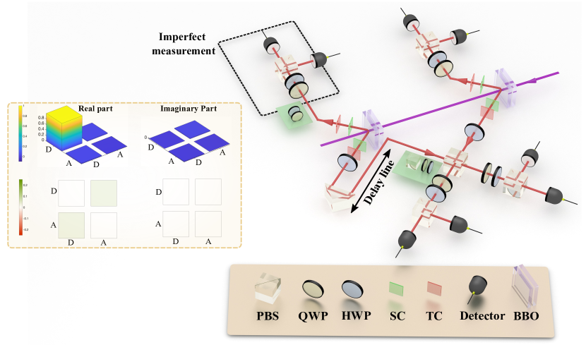
Figure 2: Sketch of the experimental setup. An ultraviolet pulse laser pumps two cascaded sandwich-like sources. The multiphoton entangled state is realized by entangling the photons emitted by each source in PBS. Additionally, a delay line is incorporated to adjust the arrival time of interfering photons. By doing so, the partial distinguishability of the photons is introduced, leading to a variable strength of the dephasing effect. For each photon distributed into different spatial paths, we employ a combination of QWP-HWP-PBS to implement single qubit local measurement. PBS: polarisation beam splitter, HWP: half-wave plate, QWP: quarter-wave plate, SC: spatial compensation crystal, TC: temporal compensation crystal. The inset depicts the tomographic results of the diagonal basis $D$, where the $(D,A)$ basis corresponds to the eigenbasis of observable $X$ with the eigenvalue of $(+1,-1)$. The difference from the idealized projector is visualized with the colored matrix present in the bottom raw.

Before discussing our experimental tests of this framework, we will briefly introduce our apparatus, leaving its detailed presentation for the Methods section. The basic ingredient of our 4-photon entangled-state source is two sandwich-like spontaneous parametric down-conversion (SPDC) sources [25, 26]. As depicted in Fig. 2, each source generates a polarization-encoded Bell pair $\left(|00\rangle+|11\rangle\right)/\sqrt{2}$, where the horizontal (vertical) polarization denotes the logic qubit 0 (1). From these two sources, we prepare a four-photon GHZ state by overlapping one photon from each source on a polarizing beamsplitter and post-selecting on finding one photon in each output port; the result of this process is a four-photon GHZ state (see the Methods for more details). In order to achieve high fidelity, we use relatively low pump powers (17 mw) to suppress noise from higher-order emission events. This yields an approximate fourfold rate of 2.5 Hz.

Following the state preparation, each photon is directed into a different path where local polarization measurements are carried out. To quantify the deviation of our experimental measurements from idealized ones, we perform a measurement tomography on the projective basis of the observables $X$ , $Y$ and $Z$, which will be used for our witness. This yields fidelities of $\mathcal{F}_{X}=99.94\pm 0.002\%$, $\mathcal{F}_{Y}=99.77\pm 0.005\%$ and $\mathcal{F}_{Z}=99.97\pm 0.002\%$ for the observables $X$ and $Y$, respectively. See the Supplementary Material for more details. These slight deviations are attributed to the misalignment of waveplates, as well as the finite extinction ratio of our PBSs. As an example, in the inset of Fig. 2, we depict the tomographic result of the $X$-basis tomography. Additionally, a theoretical analysis of the measurement inaccuracy based on a systematic error propagation is made in Supplementary Material, which is consistent with the results of our measurement tomography.

V.1 False positives from a biseparable state with small alignment errors

We have seen that imperfect measurements when used in a standard entanglement witness can lead to false positives. We begin with demonstrating this by preparing a state of four qubits which only features genuine entanglement between three of the qubits, and then we use small misalignments to achieve a false violation of the standard Mermin witness for four-qubit GME. To this end, we set out to prepare the state in Eq. (11) (See Method for details of state preparation.) Then, we artificially introduce a systematic misalignment to our measurements realising observables of the form $\widetilde{X}=qX+\sqrt{1-q^{2}}Y$ and $\widetilde{Y}=qY+\sqrt{1-q^{2}}X$, where $q=1-2\varepsilon$, instead of $X$ and $Y$.

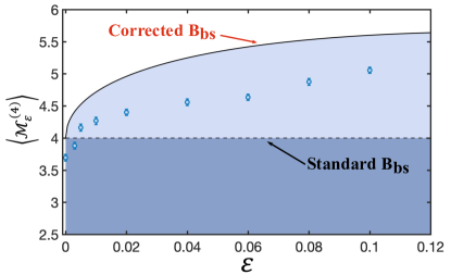
Figure 3: Experimental results for Mermin witness with misaligned measurements. The shaded areas show the biseparable regions for the standard and imperfection-adapted Mermin witness. The biseparable bound ($B_{bs}$) of standard Mermin witness is given by the dashed line. The biseparable bound corrected for imprecise measurements is given by the solid line. The dots represent the experimental value of the Mermin witness, with error bars, as obtained from a biseparable state.

The optimal strategy for creating a false positive requires us to apply the misaligned observables $\widetilde{X}$ and $\widetilde{Y}$ on the first qubit, while performing the exact observables, $X$ and $Y$, on the other three respective qubits. For simplicity, we will assume that all of of our measurements ($X$, $Y$, $\widetilde{X}$, and $\widetilde{Y}$ ) are the target measurements. This is a reasonable assumption, as we will first study a regime wherein we introduce errors on $\widetilde{X}$ and $\widetilde{Y}$ which are larger than the error in our nominal measurements of $X$ and $Y$ (which have fidelities above $99.7\%$, discussed above).

With this measurement configuration, we measured the Mermin witness for a range of imprecision parameters, from $\varepsilon=0\%$ to $\varepsilon=10\%$. In Fig. 3 we plot the experimentally observed values of the Mermin witness versus $\varepsilon$. The dashed line indicates the biseparable bound of the standard Mermin witness. Thus for any points above the shaded dark blue region, the Mermin witness would indicate the presence of four-qubit GME. In our data, already for very small measurement errors of $\varepsilon=0.5\%$, we observe a false positive. Moreover, it is expected that the amount of imprecision required for a false positive will decrease as the quality of the state preparation improves, i.e. high-quality sources are the most vulnerable since they can come close to the idealised biseparable limit. This follows from the observation that small values of $\varepsilon$ can significantly increase the witness value. This is illustrated in our data as well. The faithful implementation (i.e. when $\varepsilon=0$) shows a witness value $\langle\mathcal{M}^{(4)}_{0}\rangle=3.700\pm 0.053$ but this increases to $\langle\mathcal{M}^{(4)}_{\varepsilon}\rangle=4.178\pm 0.054$ already at $\varepsilon=0.5\%$, corresponding to a $13$ percent increase. Notably, the p-value associated with the violations of the witness is $p=1.7291\times 10^{-4}$ for $\varepsilon=0.5\%$. The solid line indicates our updated biseparble bound taking into account the measurement imprecision. We clearly see that all data points obey this corrected bound.

V.2 GME from imperfect measurements

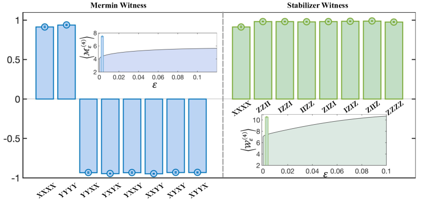
Figure 4: Experimental result of Mermin and stabilizer witness with 4-qubit GHZ state. Observed mean value for all joint expectation values in the Mermin witness. These are, respectively, $\{0.9126\pm 0.0076,0.9373\pm 0.0065,-0.9315\pm 0.0080,-0.9447\pm 0.0074,-0.9304\pm 0.0082,-0.9491\pm 0.0062,-0.9300\pm 0.0064,-0.9308\pm 0.0071\}$, and expectation values of observables in the stabilizer witness is $\{0.9126\pm 0.0076,0.9816\pm 0.0037,0.9800\pm 0.0040,0.9766\pm 0.0045,0.9800\pm 0.0042,0.9850\pm 0.0033,0.9883\pm 0.0030\}$. The left inset shows a comparison between the observed Mermin value $\langle\mathcal{M}^{(4)}\rangle=7.4665\pm 0.0212$ and the biseparable bound for imperfect measurements, and the right inset for stabilizer witness $\langle\mathcal{W}^{(4)}\rangle=10.5168\pm 0.0412$ with respect to the biseparable bound. The error bars of the data are calculated from Monte Carlo simulation which takes the Poissonian counting statistics of the detection events into account.

Using Theorem 1, we can detect GME even with imperfect measurements. To this end we convert the measurement fidelities presented above to the imprecision parameters (measurement infidelities)

$$\varepsilon_{X}\approx 6.0\times 10^{-4}$$

$$\varepsilon_{Y}\approx 2.3\times 10^{-3}$$

$$\varepsilon_{Z}\approx 3.0\times 10^{-4},$$ (14)

where $\varepsilon_{j}=1-F_{j}$. The small deviations are partly due to the imperfect retarder of waveplates during the fabrication. See the supplementary material for more details. We observe a larger error in the $Y$ basis since it is more sensitive to errors (alignment and retardance) in both the quarter- and half-waveplate. In contrast, the $X$ basis is relatively insensitive to errors in the quarter-waveplate. To complement this operational estimation, we have also estimated these parameters from simulation of the experiment and the propagation of its systematic errors; see Appendix D. The values of $\varepsilon_{X}$, $\varepsilon_{Y}$ and $\varepsilon_{Z}$ obtained from this method are comparable with the values obtained in the lab.

Using these measurements, we measure the Mermin and the stabilizer witness. In the four-qubit case, the witness operator (9) can be expressed as

$$\mathcal{M}^{(4)}_{\varepsilon} =\tilde{X}_{1}\tilde{X}_{2}\tilde{X}_{3}\tilde{X}_{4}-\tilde{X}_{1}\tilde{X}_{2}\tilde{Y}_{3}\tilde{Y}_{4}-\tilde{X}_{1}\tilde{Y}_{2}\tilde{X}_{3}\tilde{Y}_{4}$$

$$-\tilde{X}_{1}\tilde{Y}_{2}\tilde{Y}_{3}\tilde{X}_{4}-\tilde{Y}_{1}\tilde{X}_{2}\tilde{X}_{3}\tilde{Y}_{4}-\tilde{Y}_{1}\tilde{X}_{2}\tilde{Y}_{3}\tilde{X}_{4}$$

$$-\tilde{Y}_{1}\tilde{Y}_{2}\tilde{X}_{3}\tilde{X}_{4}+\tilde{Y}_{1}\tilde{Y}_{2}\tilde{Y}_{3}\tilde{Y}_{4}.$$ (15)

Our observed value for each the expectation values of each of the eight terms is displayed in Fig. 4. We estimate a Mermin witness value of $\langle\mathcal{M}^{(4)}_{\varepsilon}\rangle=7.4665\pm 0.0212$, which clearly violates the $\varepsilon$-dependent biseparable bound in Eq. (10). Setting the imprecision parameter to be our worst-case observed value in (V.2), namely $\varepsilon=2.5\times 10^{-3}$, the biseparable bound becomes $\langle\mathcal{M}^{(4)}_{\varepsilon}\rangle\leq 4.38$. The violation corresponds to 145 standard deviations. The $p$-value associated to the violation is negligible.

The stabilizer witness (12) in the four-qubit case can be expressed as

$$\mathcal{W}_{\varepsilon}^{(4)}= 4\tilde{X}_{1}\tilde{X}_{2}\tilde{X}_{3}\tilde{X}_{4}+\mathds{1}\mathds{1}\tilde{Z}_{3}\tilde{Z}_{4}+\mathds{1}\tilde{Z}_{2}\mathds{1}\tilde{Z}_{4}$$

$$+\mathds{1}\tilde{Z}_{2}\tilde{Z}_{3}\mathds{1}+\tilde{Z}_{1}\mathds{1}\mathds{1}\tilde{Z}_{4}+\tilde{Z}_{1}\mathds{1}\tilde{Z}_{3}\mathds{1}$$

$$+\tilde{Z}_{1}\tilde{Z}_{2}\mathds{1}\mathds{1}+\tilde{Z}_{1}\tilde{Z}_{2}\tilde{Z}_{3}\tilde{Z}_{4}.$$ (16)

We estimate a stabilizer witness value of $\langle\mathcal{W}^{(4)}_{\varepsilon}\rangle=10.5168\pm 0.0412$, which clearly violates the $\varepsilon$-dependent biseparable bound calculated in Appendix. C. Setting the imprecision parameter to be our worst-case observed value in (V.2), namely $\varepsilon=6\times 10^{-4}$, the biseparable bound becomes $\langle\mathcal{W}^{(4)}_{\varepsilon}\rangle\leq 7.19$. The violation corresponds to 81 standard deviations. The $p$-value associated to the violation is negligible.

V.3 Fidelity estimation from imperfect measurements

An important feature of both the standard Mermin witness and the stabilizer witness is that they can also be used to bound the fidelity between the source state and the targeted GHZ state. Specifically, assuming exact measurements, the fidelity can be bounded as $F_{\text{ghz}}(\rho)\geq\frac{\langle\mathcal{M}^{(4)}_{0}\rangle}{8}\equiv L^{\mathcal{M}}_{0}$ and $F_{\text{ghz}}(\rho)\geq\frac{\langle\mathcal{W}^{(4)}_{0}-3\rangle}{8}\equiv L^{\mathcal{W}}_{0}$ respectively. Since the fidelity is a standard tool for benchmarking the quality of a state preparation, we now consider how the lower bounds must be revised, into functions $L^{\mathcal{W}}_{\varepsilon}$ and $L^{\mathcal{M}}_{\varepsilon}$, as a consequence of imperfect measurements. To this end, we have employed one imprecision parameter per basis, whose value is fixed to that experimentally obtained in Eq. (V.2). Then, we have numerically searched for the smallest value of $F_{\text{ghz}}$ compatible with a given value of the Mermin and stabilizer witness under imperfect measurements. This corresponds to an estimate of $L^{\mathcal{W}}_{\varepsilon}$ and $L^{\mathcal{M}}_{\varepsilon}$ respectively. The fidelity bound is illustrated in Fig. 5, where $L_{0}$ (dashed) and the numerically estimated $L_{\varepsilon}$ (continuous) are plotted versus the observed fraction of the maximal Mermin and stabilizer witness value, as the blue and orange curves, respectively. We see that in spite of the tiny experimental imprecision parameters, there is a significant difference between the estimated fidelity that we can claim from our realistic measurements and that we could claim if we assumed our measurements were ideal. In particular, if we assume ideal measurements we could claim a fidelity of $93.25\%$ for the Mermin witness and $93.96\%$ for the stabilizer witness; however, given our measurement imperfections we can only claim a fidelity of $86.61\%$ and $88.07\%$ respectively.

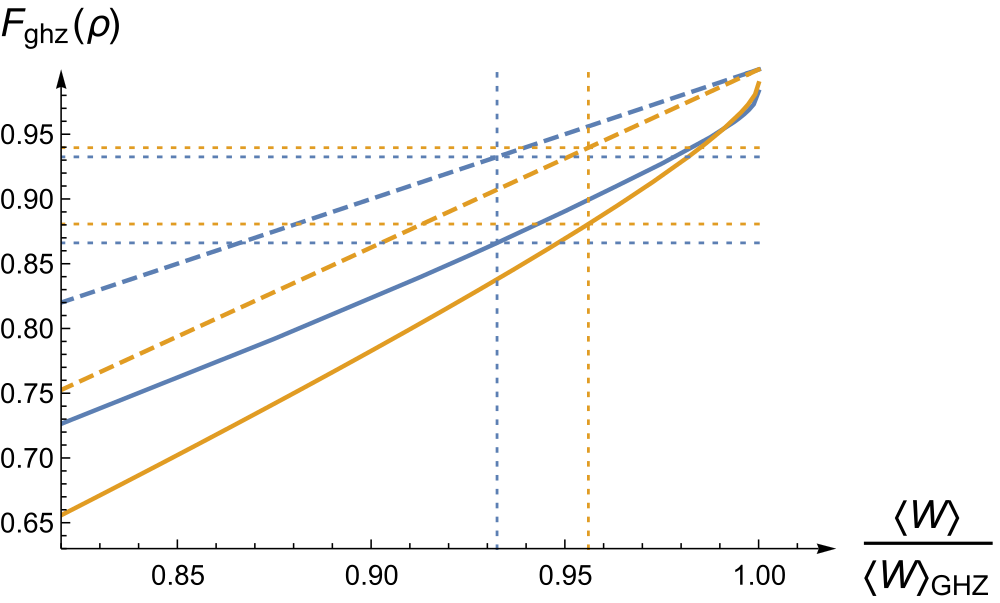
Figure 5: Fidelity estimation with imperfect measurements. Numerical lower bound on the GHZ-fidelity of a four-qubit state versus the fraction of the optimal value obtained by a GHZ-state. The Mermin witness (V.2) in blue and the stabilizer witness (V.2) in orange are evaluated at the experimentally observed imprecision parameters (V.2). The dashed lines show the respective fidelity values without considering measurement imperfections and the dotted vertical lines show the values $0.9325$ and $0.9561$ obtained in the experiment.

V.4 Robustness hierarchy

The imperfect measurement framework is an attempt at modelling realistic measurement errors in an operational way, without resorting to a black-box picture. Consequently, the deductions are made with much more knowledge in hand than from device-independent inference. This suggests that the decreasingly powerful frameworks, namely device-independence, imperfect measurements and idealised measurements should, respectively, be increasingly successful at detecting weakly entangled states. We now study this intuition for the most relevant form of noise in our setup for four qubits. We verify that the imperfect measurement framework permits the detection of states that are device-independently not detected with standard witnesses in the literature.

Dephasing is a dominant type of noise in many state-preparation devices. This is also the case in our four-photon GHZ source, specifically corresponding to imperfections in the Hong-Ou-Mandel interference at the PBS. Imperfect interference induces distinguishability in the form of dephasing noise. That corresponds to a noisy GHZ state of the form

$$\rho_{\text{deph}}(p)=p\outerproduct{\text{ghz}}{\text{ghz}}+(1-p)\outerproduct{\text{ghz}^{-}}{\text{ghz}^{-}},$$ (17)

where the $|\text{ghz}^{-}\rangle=(|0\rangle^{\otimes 4}-|1\rangle^{\otimes 4})/\sqrt{2}$, and $p\in[0,1]$ quantifies the quality of the source. In our experiment, we use a delay line to tune the arrival time of one of the interfering photons, see Fig. 2(b). This enables us to vary the strength of the dephasing. We have measured the Mermin witness for several different values of the visibility $p$. In order to showcase the relevance of our argument beyond the relatively small imperfections (V.2) reported for our specific setup, we have conservatively estimated our imprecision parameters to be significantly larger. In Fig 6, we plot the measured Mermin witness values (blue-colored data) versus $p$ along with the biseparable bound, evaluated at $\varepsilon=0.5\%$. We identify the point at which this threshold is exceeded (shaded area). We find that we can detect GME down to values of $p=79.4\%$, which agrees very well with the theoretical value of $p=78.3\%$. For the sampled states below $p=79.4\%$ we can no longer conclude that the state possesses any GME. Furthermore, we have also measured the stabilizer witnesses with the same evaluated imperfection level (orange-coloured data). For all sampled dephased four-qubit states, the stabilizer witness values are well above the biseparable bound. See Appendix F for details on the noise robustness of the Mermin and stabiliser witnesses.

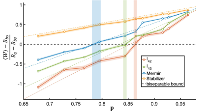
Figure 6: Experimental results of robustness comparison between the device-independent witness, modified Mermin witness, and stabilizer witness. The horizontal axis represents the visibility $p$ of the GHZ state in Eq. (17). The threshold visibility at which GME is detected is illustrated separately for a device-independent witness with two ($I_{42}$) and three ($I_{43}$) local settings, the Mermin witness and stabilizer witness with $\varepsilon=0.5\%$ imprecise measurements. Experimental data are plotted by dots while errorbars are described with shadows around the dots. For the convenience of comparison, we normalize the witness value $\langle\mathcal{W}\rangle$ into $\frac{\langle\mathcal{W}\rangle-B_{bs}}{B_{q}-B_{bs}}$, thus the biseparable bound is always 0 and the maximal violation allowed by quantum theory is always 1, where the $B_{bs}$ is biseparable bound while the $B_{q}$ is quantum bound.

To compare our approach with a device-independent detection of GME, we use a witness that was introduced in [11, 27] and experimentally demonstrated in ref. [13]. This is a witness for an $n$-partite quantum system with $m$ possible choices of local measurement settings per party and is defined as

$$I_{nm}=\sum\limits_{s\equiv 0(mod\,m)}(-1)^{s/m}E_{s}+\sum\limits_{s\equiv 1(mod\,m)}(-1)^{(s-1)/m}E_{s}$$ (18)

where $E_{s}=\sum_{\vec{\mathbf{r}}}(-1)^{r}P(\vec{\mathbf{r}}|\vec{\mathbf{s}})$ is the $n-$partite correlator; the vector $\vec{\mathbf{s}}=(s_{1},s_{2},\cdots s_{n})\in\{0,1,\cdots m-1\}$ and $\vec{\mathbf{r}}=(r_{1},r_{2},\cdots r_{n})\in\{0,1\}$ respectively describes the inputs and outputs of measurement settings, while $s=\sum_{j}s_{j}$, $r=\sum_{j}r_{j}$. Specifically, the $j$-th party of state freely chooses one of $m$ possible measurement settings and indexes it with $s_{j}\in\{0,1,\cdots m-1\}$, and the local measurement gives a binary output $r_{j}\in\{0,1\}$. The corresponding conditional probability is $P(\vec{\mathbf{r}}|\vec{\mathbf{s}})$.

We again use our four-qubit source to investigate the effect of detecting GME on dephased GHZ-states using $I_{nm}$. In Fig. 6 we plot the results for $m=2$ (red-colored points) and $m=3$ (green-colored points) inputs per party, respectively, as a function of the visibility $p$. The black dashed lines in the plots represent the biseparable bound, above which GME is certified. For the convenience of comparison, we also identify the point at which this threshold is exceeded, highlighting them with shaded areas. With two and three settings per party, we achieve a violation above $p=86.4\%$ and $p=84.3\%$, respectively. These values agree well with the theoretical predictions $p=85.4\%$ and $p=83.4\%$, respectively. These are both notably lower amounts of noise than we found for the revised Mermin witness, even using a measurement imperfection significantly higher than we observed in the lab. This illustrates how the device-independent approach while excluding concerns of device control, comes at an additional price in terms of the detectable GME. By exploiting easily available knowledge about the apparatus, here the imprecision parameter, the utility of the device is significantly improved, while still doing away with the unwarranted idealisations standard entanglement witnesses.

VI Discussion

Verifying genuine multipartite entanglement is an important building block for quantum computers and quantum networks. This requires good control of the quantum measurement devices. As illustrated here, small deviations in the fidelity of these measurements, at scales that are relevant for state-of-the-art photonic experiments, can significantly undermine such verification. This pertains both to the use of entanglement witnesses to detect GME and to their use for estimating the fidelity of the state preparation device. Imperfect measurements are inevitable and while our experiment focuses on photonics, their relevance extends to other platforms too. In particular, due to the relevance of cross-talk between adjacent qubits, it might be of special relevance in atomic systems [28, 13, 29, 30] and superconducting qubits [31, 32, 33]. Another frontier where measurement imperfections are particularly relevant is in high-dimensional quantum systems [34, 35], where it is often the case that control over the measurement decreases with the dimensionality.

In our work, we have focused mainly on GHZ states, analytically corrected a relevant family of entanglement witnesses, and demonstrated their relevance in the experiment. However, optimally correcting entanglement witnesses for measurement imperfections seems in general to be a hard task. An interesting open problem is if this can be achieved systematically, in an efficient manner. That would permit a rigorous analysis of more generic entanglement witnesses, tailored for a variety of different multipartite states, and their adaptation to experiment. In Appendix E we have numerically explored some well-known entanglement witnesses for a three and four qubits, in a W-state and cluster state. The results are qualitatively similar to those presented for the GHZ states.

Furthermore, one should note that there are many ways of modeling imperfect measurements. Our approach here, which builds on a series of related previous works [9, 10, 24], has the advantage that it is operationally meaningful, does not require any detailed physical modeling, is not limited to a specific physical platform and requires a small resource cost for its estimation. However, for specific physical systems, it may be possible to provide well-motivated models that are more conservative, taking the specific physics of the platform into account, without requiring extensive noise tomography. This can make possible an analysis of entanglement verification under imperfect measurements in which the cost of imperfections is reduced. An alternative route to reducing that cost, while continuing to not require detailed physical modeling, is to increase the resources spent in probing the measurement devices, i.e. to not base the lab measurement only on their target fidelity but also on additional trusted parameters that now require estimation in the lab. In general, approaches in the spirit presented here represent an interesting and practically relevant middle-way between standard entanglement witnessing and device-independent entanglement certification.

VII Methods

Sandwiched-like EPR source. The two cascaded sandwiched-like EPR sources are pumped by a 390 nm ultraviolet light which is generated via a frequency doubler with a mode-locked Ti: sapphire femtosecond laser of 780 nm central wavelength. Each EPR source consists of a true zero order half wave plate (THWP) sandwiched by two identical 1mm-thick beta barium borate (BBO) crystals with the type-II beam-like cutting type. Each BBO crystal produces the down-converted photons with the state of $|H_{1}V_{2}\rangle$, while the photon pair in the first BBO is transformed into $|V_{1}H_{2}\rangle$ by the THWP. Superposition of the SPDC processes in two BBOs is made by applying a temporal and spatial compensation crystal in each photon path, which makes the two possible ways of down conversion indistinguishable, leading to the final state $\left(|H_{1}V_{2}\rangle+|V_{1}H_{2}\rangle\right)/\sqrt{2}$.

Four-qubit state generation. The four-qubit GHZ state is prepared by interfering the indistinguishable photons from EPR pairs. As shown in Fig. 2, one of the photons in each EPR pair is directed into the PBS, which behaves as a parity check operator $|00\rangle\langle 00|+|11\rangle\langle 11|$ by postselecting the case where both of the photons are transmitted or reflected by PBS. With the overlap of arriving photons in PBS, the Hong-Ou-Mandel interference occurs. By entangling the two identical sources, The four-qubit GHZ state $|\mathrm{GHZ_{4}}\rangle=\left(|0\rangle^{\otimes 4}+|1\rangle^{\otimes 4}\right)/\sqrt{2}$ is prepared.

The biseparable state for demonstrating the violation of the standard Mermin witness is comprised of one qubit state and a three-qubit GHZ state. The state preparation is based on the setup while one PBS is applied to one of the sources to postselect the separable state $|01\rangle$ generated by only one of BBO. The following local unitaries are applied to transform the separable state into $U_{1}\otimes U_{2}|01\rangle=\frac{1}{2}\left(|0\rangle+e^{i\pi/4}|1\rangle\right)\left(|0\rangle+e^{-i\pi/4}|1\rangle\right)$. Similarly as four-qubit GHZ, the separable state interferes with the second EPR source via Hong-Ou-Mandel effect in PBS, yielding the desired state $|\psi\rangle=(|0\rangle+\mathrm{e}^{i\pi/4}|1\rangle)(|0\rangle^{\otimes 3}+\mathrm{e}^{-i\pi/4}|1\rangle^{\otimes 3})/2$.

VIII Acknowledgements

S.M. is supported by the Basque Government through IKUR strategy and through the BERC 2022-2025 program and by the Ministry of Science and Innovation: BCAM Severo Ochoa accreditation CEX2021-001142-S / MICIN / AEI / 10.13039/501100011033. A.T. is supported by the Wenner-Gren Foundation and by the Knut and Alice Wallenberg Foundation through the Wallenberg Center for Quantum Technology (WACQT). P.W., L.R and H.C are supported by the European Union’s Horizon 2020 research and innovation programme under grant agreement No 820474 (UNIQORN) and No 899368) (EPIQUS); the Austrian Science Fund (FWF) through [F7113] (BeyondC), and [FG5] (Research Group 5); the AFOSR via FA9550-21- 1-0355 (QTRUST); the QuantERA II Programme under Grant Agreement No 101017733 (PhoMemtor); the Austrian Federal Ministry for Digital and Economic Affairs, the National Foundation for Research, Technology and Development and the Christian Doppler Research Association. C.Z. is supported by the Fundamental Research Funds for the Central Universities (Nos. WK2030000061, YD2030002015), the National Natural Science Foundation of China (No. 62075208).

Appendix A Proof of the theorem

Let $A_{0}^{(k)}$ and $A_{1}^{(k)}$ be two dichotomic observables for party $k$ padded with the identity operator on all other parties and define the following observables recursively

$$M_{1} =A_{0}^{(1)}$$ (A.1)

$$N_{1} =A_{1}^{(1)}$$ (A.2)

$$M_{k} =M_{k-1}A_{0}^{(k)}-N_{k-1}A_{1}^{(k)}$$ (A.3)

$$N_{k} =M_{k-1}A_{1}^{(k)}+N_{k-1}A_{0}^{(k)}.$$ (A.4)

Then it holds that

$$M_{k} =\tfrac{1}{2}\bigg{(}\prod\limits_{j=1}^{k}(A_{0}^{(j)}+iA_{1}^{(j)})+\prod\limits_{j=1}^{k}(A_{0}^{(j)}-iA_{1}^{(j)})\bigg{)}$$ (A.5)

$$N_{k} =\tfrac{-i}{2}\bigg{(}\prod\limits_{j=1}^{k}(A_{0}^{(j)}+iA_{1}^{(j)})-\prod\limits_{j=1}^{k}(A_{0}^{(j)}-iA_{1}^{(j)})\bigg{)}.$$ (A.6)

It certainly holds for $k=2$ and therefore we can inductively conclude

$$M_{k}= M_{k-1}A_{0}^{(k)}-N_{k-1}A_{1}^{(k)}$$

$$= \tfrac{1}{2}\bigg{(}\prod\limits_{j=1}^{k-1}(A_{0}^{(j)}+iA_{1}^{(j)})+\prod\limits_{j=1}^{k-1}(A_{0}^{(j)}-iA_{1}^{(j)})\bigg{)}A_{0}^{(k)}$$

$$+\tfrac{i}{2}\bigg{(}\prod\limits_{j=1}^{k-1}(A_{0}^{(j)}+iA_{1}^{(j)})-\prod\limits_{j=1}^{k-1}(A_{0}^{(j)}-iA_{1}^{(j)})\bigg{)}A_{1}^{(k)}$$

$$= \tfrac{1}{2}\bigg{(}\prod\limits_{j=1}^{k-1}(A_{0}^{(j)}+iA_{1}^{(j)})(A_{0}^{(k)}+iA_{1}^{(k)})$$

$$+\prod\limits_{j=1}^{k-1}(A_{0}^{(j)}-iA_{1}^{(j)})(A_{0}^{(k)}-iA_{1}^{(k)})\bigg{)}$$

$$= \tfrac{1}{2}\bigg{(}\prod\limits_{j=1}^{k}(A_{0}^{(j)}+iA_{1}^{(j)})+\prod\limits_{j=1}^{k}(A_{0}^{(j)}-iA_{1}^{(j)})\bigg{)}$$

and analogously for $N_{k}$.

It further holds that

$$M_{k}=M_{k-l}M_{l}-N_{k-l}N_{l},$$ (A.7)

up to proper relabelling of the parties, where $M_{k-l}$ and $N_{k-l}$ act on party 1 to $k-l$ and $M_{l}$ and $N_{l}$ act on party $k-l+1$ to $k$. For $l=1$ this follows directly from the definition, so the statement follows inductively

$$M_{k}= M_{k-l}M_{l}-N_{k-l}N_{l}$$

$$= M_{k-l-1}A_{0}M_{l}-N_{k-l-1}A_{1}M_{l}$$

$$-M_{k-l-1}A_{1}N_{l}-N_{k-l-1}A_{0}N_{l}$$

$$= M_{k-l-1}(A_{0}M_{l}-A_{1}N_{l})-N_{k-l-1}(A_{1}M_{l}+A_{0}N_{l})$$

$$= M_{k-l-1}M_{l+1}-N_{k-l-1}N_{l+1}$$

after proper relabelling of the party numbers.

Following Uffink [36], who proved this result for $k=2$, we show that for $k\geq 2$

$$\langle M_{k}\rangle^{2}+\langle N_{k}\rangle^{2}\leq 2^{2k-2}.$$ (A.8)

This follows from

$$\sup(\langle M_{k}\rangle^{2}+\langle N_{k}\rangle^{2})$$

$$= \sup(\langle M_{k-1}A_{0}^{(k)}-N_{k-1}A_{1}^{(k)}\rangle^{2}+\langle M_{k-1}A_{1}^{(k)}+N_{k-1}A_{0}^{(k)}\rangle^{2})$$

$$= \sup(\langle M_{k-1}A_{0}^{(k)}\rangle^{2}+\langle N_{k-1}A_{1}^{(k)}\rangle^{2}-2\langle M_{k-1}A_{0}^{(k)}\rangle\langle N_{k-1}A_{1}^{(k)}\rangle$$

$$+\langle M_{k-1}A_{1}^{(k)}\rangle^{2}+\langle N_{k-1}A_{0}^{(k)}\rangle^{2}+2\langle M_{k-1}A_{1}^{(k)}\rangle\langle N_{k-1}A_{0}^{(k)}\rangle)$$

$$\leq \sup(\langle M_{k-1}A_{0}^{(k)}\rangle^{2}+\langle N_{k-1}A_{1}^{(k)}\rangle^{2}+\langle M_{k-1}A_{1}^{(k)}\rangle^{2}+\langle N_{k-1}A_{0}^{(k)}\rangle^{2})$$

$$+2\sup(\langle M_{k-1}A_{1}^{(k)}\rangle\langle N_{k-1}A_{0}^{(k)}\rangle-\langle M_{k-1}A_{0}^{(k)}\rangle\langle N_{k-1}A_{1}^{(k)}\rangle)$$

$$\leq 2\sup(\langle M_{k-1}\rangle^{2}+\langle N_{k-1}\rangle^{2})+4\sup(|\langle M_{k-1}\rangle\langle N_{k-1}\rangle|)$$

$$\leq 4\sup(\langle M_{k-1}\rangle^{2}+\langle N_{k-1}\rangle^{2})$$

$$\leq 2^{2k-2}.$$

Uffink [36] proved a similar result in the same way, that coincides with this one for $k$ odd.

Since the previous inequality holds for all points on a disc, also every tangential inequality of the form

$$\alpha\langle M_{k}\rangle+\beta\langle N_{k}\rangle\leq 2^{k-1}\sqrt{\alpha^{2}+\beta^{2}}$$ (A.9)

holds for all $\alpha$ and $\beta$.

Since the Mermin witness in Eq. (9) is linear, its maximal value is attained for pure states. First, assume that we have a biseparable $n$-qubit state where each partition has more than one qubit. Then from Eq. (A.7) it follows that

$$\langle M_{n}\rangle =\langle M_{n-l}\rangle\langle M_{l}\rangle-\langle N_{n-l}\rangle\langle N_{l}\rangle$$ (A.10)

$$\leq 2^{n-l-1}\sqrt{\langle M_{l}\rangle^{2}+\langle N_{l}\rangle^{2}}$$ (A.11)

$$\leq 2^{n-l-1}2^{l-1}=2^{n-2},$$ (A.12)

where we have first used Eq. (A.9) and then Eq. (A.8). This is a remarkable result, it shows that the Mermin witness is completely robust against misalignment of the measurement direction, as long as the biseparable partition includes more than a single qubit in each set.

Next, we assume that only one qubit, without loss of generality, say the $n$-th qubit, is separable from the rest, such that

$$\langle M_{n}\rangle =\langle A_{0}^{(n)}\rangle\langle M_{n-1}\rangle-\langle A_{1}^{(n)}\rangle\langle N_{n-1}\rangle$$

$$\leq 2^{n-2}\sqrt{\langle A_{0}^{(n)}\rangle^{2}+\langle A_{1}^{(n)}\rangle^{2}}.$$ (A.13)

To maximise the inequality from Eq. (A) while satisfying the condition $A_{0}^{(n)}=qX+\sqrt{1-q^{2}}X^{\perp}$ and $A_{1}^{(n)}=qY+\sqrt{1-q^{2}}Y^{\perp}$ with $q\geq 1-2\varepsilon$, we can choose $X^{\perp}=Y$ and $X^{\perp}=Y$. Therefore it follows

$$\sqrt{\langle A_{0}^{(n)}\rangle^{2}+\langle A_{1}^{(n)}\rangle^{2}}$$ (A.14)

$$= \sqrt{\langle X\rangle^{2}+\langle Y\rangle^{2}+4q\sqrt{1-q^{2}}\langle X\rangle\langle Y\rangle}$$ (A.15)

$$\leq \sqrt{1+2q\sqrt{1-q^{2}}}$$ (A.16)

$$= (q+\sqrt{1-q^{2}})$$ (A.17)

$$\leq 1-2\varepsilon+2\sqrt{\varepsilon(1-\varepsilon)}$$ (A.18)

for $\varepsilon\leq(2-\sqrt{2})/4$, where we have used $\langle X\rangle^{2}+\langle Y\rangle^{2}\leq 1$ and $\langle X\rangle\langle Y\rangle\leq 1/2$. This proves the bound given in Eq. (10).

Assume now that party 1 performs the measurements $A_{0}^{(1)}=(1-2\varepsilon)X+2\sqrt{\varepsilon(1-\varepsilon)}Y$ and $A_{1}^{(1)}=(1-2\varepsilon)Y+2\sqrt{\varepsilon(1-\varepsilon)}X$, while all other parties perform the measurements $A_{0}^{(k)}=X$ and $A_{1}^{(k)}=Y$. In this case the state defined in Eq. (11) saturates the bound.

Appendix B Analysis of the biseparable bound for the stabilizer witness

Define the operators

$$M_{k} =2^{k-2}\prod\limits_{j=1}^{k}A_{0}^{(j)}$$ (B.1)

$$N_{k} =\prod\limits_{j=2}^{k}(A_{1}^{(j-i)}A_{1}^{(j)}-\mathds{1}),$$ (B.2)

where again $A_{0}^{(j)}$ and $A_{1}^{(j)}$ are two dichotomic observables for party $j$ padded with the identity operator on all other parties. It is clear that for $k\geq 2$ it holds

$$\langle M_{k}\rangle^{2}+c^{2}\langle N_{k}\rangle^{2}\leq 2^{2k-4}+2^{2k-2}=2^{2k-4}(4c^{2}+1).$$ (B.3)

As before, also every tangential inequality of the form

$$\alpha\langle M_{k}\rangle+\beta c\langle N_{k}\rangle\leq 2^{k-2}\sqrt{4c^{2}+1}\sqrt{\alpha^{2}+\beta^{2}}$$ (B.4)

holds for all $\alpha$ and $\beta$. Assume now that we have a biseparable pure $n$-qubit state, where each partition has more than a single qubit. Then it follows that

$$\langle M_{n}\rangle+\langle N_{n}\rangle \leq\langle M_{n-l}\rangle\langle M_{l}\rangle+2\langle N_{n-l}\rangle\langle N_{l}\rangle$$ (B.5)

$$\leq 3\times 2^{n-l-3}\sqrt{\langle M_{l}\rangle^{2}+2\langle N_{l}\rangle^{2}}$$ (B.6)

$$\leq 9\times 2^{n-4},$$ (B.7)

where we have first used Eq. (B.4) and then Eq. (B.3), both with $c=\sqrt{2}$. Since the stabilizer witness with measurement operators $A_{0}^{(j)}$ and $A_{1}^{(j)}$ is just

$$\mathcal{W}^{(n)}=M_{n}+N_{n}-\mathds{1},$$ (B.8)

it follows that the expectation value for a biseparable pure state with each partition including at least 2 qubits can not surpass the value $9\times 2^{n-4}-1$, independent of the assumed error in the measurements. This value is just slightly larger than the biseparable bound for idealised measurements, see Fig. A.1 and A.2. Therefore we focus on biseparable states where only a single party is separable from the rest.

Appendix C The stabilizer witness for $n=3$ and $n=4$

Here we explicitely calculate the biseparable bound for the stabiliizer witness with imprecise measurements, that is, we compute the maximal expectation value of biseparable states defined in Eq. (12). This would in principle involve a optimization over all parameters $q_{j}\geq 1-2\varepsilon$ and all perpendicular observables $\{X_{j}^{\perp}\}$ and $\{Y_{j}^{\perp}\}$. Following the discussion in Section IV.2, we can reduce the problem by assuming $\tilde{X}_{j}=q_{j}X+\sqrt{1-q_{j}^{2}}Z$, $\tilde{Z}_{j}=q_{j}Z+\sqrt{1-q_{j}^{2}}X$ and $q_{j}=1-2\varepsilon$ for all $j$. Further we assume that the state has the form $|\psi\rangle=|\chi_{A}\rangle|\psi_{BC}\rangle$ with $|\chi(\theta)\rangle=\cos{\theta}|0\rangle+\sin{\theta}|1\rangle$. This then results in

$$\langle\chi(\theta)|\tilde{X}_{1}|\chi(\theta)\rangle =2\sqrt{\varepsilon(1-\varepsilon)}\cos{2\theta}+(1-2\varepsilon)\sin{2\theta}$$ (C.1)

$$\langle\chi(\theta)|\tilde{Z}_{1}|\chi(\theta)\rangle =(1-2\varepsilon)\cos{2\theta}+2\sqrt{\varepsilon(1-\varepsilon)}\sin{2\theta}.$$ (C.2)

For $n=3$ the stabilizer witness of Eq. (7) with imprecise measurements becomes

$$\mathcal{W}^{(3)}_{\varepsilon}= 2\tilde{X}_{1}\tilde{X}_{2}\tilde{X}_{3}+\mathds{1}\tilde{Z}_{2}\tilde{Z}_{3}+\tilde{Z}_{1}\mathds{1}\tilde{Z}_{3}+\tilde{Z}_{1}\tilde{Z}_{2}\mathds{1}.$$ (C.3)

We therefore compute the maximal eigenvalue of

$$2\langle\tilde{X}_{1}\rangle\tilde{X}_{2}\tilde{X}_{3}+\langle\tilde{Z}_{1}\rangle(\mathds{1}\tilde{Z}_{3}+\tilde{Z}_{2}\mathds{1})+\tilde{Z}_{2}\tilde{Z}_{3},$$ (C.4)

and optimise over $\theta$. The result, which admits no closed expression, is shown as the green line in Fig. A.1.

Assuming errors in the measurements are only present in one party, the biseparable bound is given by the largest eigenvalue of

$$\langle\tilde{X}_{1}\rangle XX+\langle\tilde{Z}_{1}\rangle(\mathds{1}Z+Z\mathds{1})+ZZ.$$ (C.5)

Optimizing over $\theta$ we obtain $1+2\sqrt{1+4(1-2\varepsilon)\sqrt{\varepsilon(1-\varepsilon)}})$, shown in blue in Fig. A.1. We notice that for small errors $\epsilon$ this curve has the same scaling as the optimal bound.

Assuming a fully separable state $|\psi\rangle=|\chi(\theta)\rangle|\chi(\theta)\rangle|\chi(\theta)\rangle$ and $\theta=\pi/8$ we have

$$\langle W_{\varepsilon}^{(3)}\rangle= \frac{3}{2}(1+\sqrt{2})-3\sqrt{2}\varepsilon-\sqrt{2}(1-2\varepsilon)^{3}$$ (C.6)

$$+2(3+\frac{\sqrt{2}}{2}-6\varepsilon+\sqrt{2}(1-2\varepsilon)^{2})\sqrt{\varepsilon(1-\varepsilon)},$$

which is the maximal value achievable for fully separable states. It is shown in yellow in Fig. A.1 and it approximates the optimal bound for large errors close to $\epsilon=\tfrac{2-\sqrt{2}}{4}$.

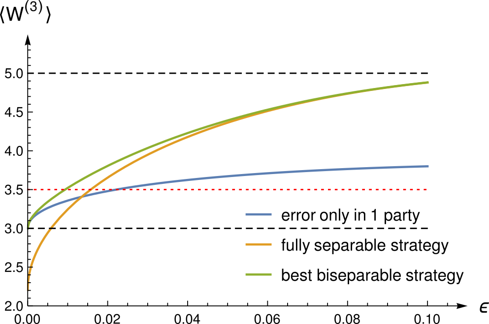
Figure A.1: Separable bounds of the stabilizer witness for three qubits. The figure shows the separable bound of the stabilizer witness $\mathcal{W}^{(3)}$ from Eq. (C.3) with various assumptions of imprecision and separability. The biseparable bound assuming imprecise measurements in only one party is shown in blue, whereas the fully separable bound assuming imprecise measurements in all three parties is shown in orange. In green we have the maximal attainable value for biseparable states assuming imprecise measurements in all three parties. The dashed black lines show the biseparable and the quantum bound for accurate measurements and the dotted red line shows the bound of $9\times 2^{n-4}-1$ for biseparable strategies splitting more than a single qubit.

For $n=4$ the witness becomes

$$\mathcal{W}_{\varepsilon}^{(4)}= 4\tilde{X}_{1}\tilde{X}_{2}\tilde{X}_{3}\tilde{X}_{4}+\mathds{1}\mathds{1}\tilde{Z}_{3}\tilde{Z}_{4}+\mathds{1}\tilde{Z}_{2}\mathds{1}\tilde{Z}_{4}$$

$$+\mathds{1}\tilde{Z}_{2}\tilde{Z}_{3}\mathds{1}+\tilde{Z}_{1}\mathds{1}\mathds{1}\tilde{Z}_{4}+\tilde{Z}_{1}\mathds{1}\tilde{Z}_{3}\mathds{1}$$

$$+\tilde{Z}_{1}\tilde{Z}_{2}\mathds{1}\mathds{1}+\tilde{Z}_{1}\tilde{Z}_{2}\tilde{Z}_{3}\tilde{Z}_{4}.$$ (C.7)

We therefore compute the maximal eigenvalue of

$$4\langle\tilde{X}_{1}\rangle\tilde{X}_{2}\tilde{X}_{3}\tilde{X}_{4}+\mathds{1}\tilde{Z}_{3}\tilde{Z}_{4}+\tilde{Z}_{2}\mathds{1}\tilde{Z}_{4}+\tilde{Z}_{2}\tilde{Z}_{3}\mathds{1}$$

$$+\langle\tilde{Z}_{1}\rangle(\mathds{1}\mathds{1}\tilde{Z}_{4}+\mathds{1}\tilde{Z}_{3}\mathds{1}+\tilde{Z}_{2}\mathds{1}\mathds{1}+\tilde{Z}_{2}\tilde{Z}_{3}\tilde{Z}_{4}),$$ (C.8)

and maximise over $\theta$. The result, which admits no closed expression, is shown as the green line in Fig. A.2.

Assuming that imprecisions are only present in one party, we calculate the largest eigenvalue of

$$4\langle\tilde{X}_{1}\rangle XXX+\mathds{1}ZZ+Z\mathds{1}Z+ZZ\mathds{1}$$ (C.9)

$$+\langle\tilde{Z}_{1}\rangle(\mathds{1}\mathds{1}Z+\mathds{1}Z\mathds{1}+\mathds{1}Z\mathds{1}+ZZZ),$$

and optimise over $\theta$, which results in $3+4\sqrt{1+4(1-2)\varepsilon\sqrt{\varepsilon(1-\varepsilon)}}$ for $\theta=\pi/8$, shown as blue line in Fig. A.2. This case is a good approximation to the biseparable bound for small values of $\varepsilon$.

For large misalignment errors $\varepsilon$, we find that the expectation value of the fully separable state $|\psi\rangle=|\chi(\pi/8)\rangle|\chi(\pi/8)\rangle|\chi(\pi/8)\rangle|\chi(\pi/8)\rangle$ assuming equally imprecise measurements in all parties is $\frac{17}{4}+20\varepsilon(1-\varepsilon)(1-2\varepsilon)^{2}+22(1-2\varepsilon)\sqrt{\varepsilon(1-\varepsilon)}$, which approaches the biseparable bound for large errors close to $\epsilon=\tfrac{2-\sqrt{2}}{4}$. It is shown in yellow in Fig. A.2.

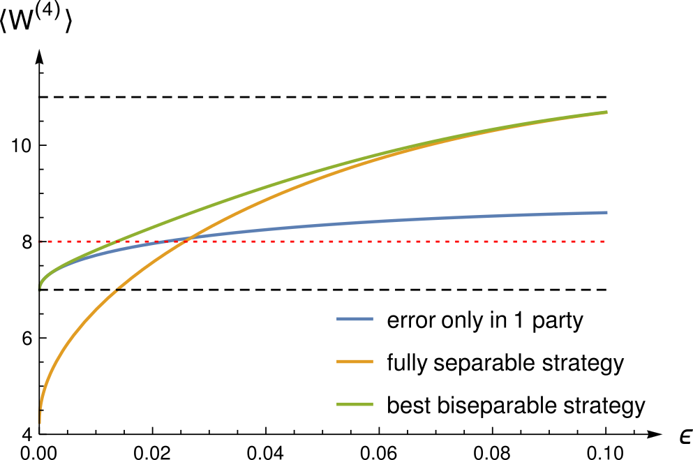
Figure A.2: Separable bounds of the stabilizer witness for four qubits. The figure shows the separable bound of the stabilizer witness $\mathcal{W}^{(4)}$ from Eq. (C) with various assumptions of imprecision and separability. The green line is the conjectured optimum. On the two extremes we have in blue the case where only the measurements in the party that is separated from the rest are altered, whereas in orange we have the bound for fully separable states. The quantum bound is shown in red, it is reached both by biseparable and fully separable states for high enough misalignments in the measurement direction. The dashed black lines show the biseparable and the quantum bound for accurate measurements and the dotted red line shows the bound of $9\times 2^{n-4}-1$ for biseparable strategies splitting more than a single qubit.

Appendix D Error analysis of lab observables

Characterizing the imperfection of the implemented measurement (lab observables) is a prerequisite for developing the corrected bi-separable bound of our protocol. In this section, the theoretical model of measurement imperfection is given.

State preparation	$|H\rangle$	$|V\rangle$	$|D\rangle$	$|A\rangle$	$|R\rangle$	$|L\rangle$	Fidelity
Projector $|D\rangle$	183295	156835	346731	96	164614	182170	0.9994$\pm$0.00001
Projector $|A\rangle$	166765	191123	180	348779	182989	164313	0.9994$\pm$0.00001
Projector $|R\rangle$	176340	170533	190799	153178	342721	1586	0.9976$\pm$0.00005
Projector $|L\rangle$	168310	175173	154604	191831	1690	338662	0.9977$\pm$0.00006
Projector $|H\rangle$	362365	188	182419	181078	186949	179468	0.9997$\pm$0.00002
Projector $|V\rangle$	144	370981	180420	179439	178401	185962	0.9998$\pm$0.00002

Table 1: Raw data of measurement tomography.

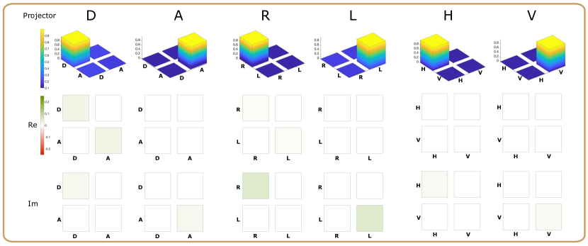
Figure A.3: Tomographic results of projectors. Here the projector $(D,A)$ basis corresponds to the eigenbasis of observable $X$ with the eigenvalue of $(+1,-1)$, while the $(R,L)$ corresponds to observable $Y$ and the $(H,V)$ corresponds to observable $Z$. The real part of the tomographic matrix is depicted in the first raw. For a clear comparison with ideal projectors, the difference between the tomographic projectors and ideal projectors are presented in the second (real part) and third (imaginary part) raw.

The systematic error propagation takes the finite extinction ratio of PBS, the misalignment of the motorized rotation stage for waveplates, and the imperfect retarder of waveplates into account. An ideal PBS would transmit horizontal polarization (encoded as $|0\rangle$) and totally reflect vertical polarization (encoded as $|1\rangle$). Then the target measurement basis, defined as a combination of QWP, HWP and transmitted outcome of PBS, would be $|\psi\left(\theta,\phi\right)\rangle$ ($|\psi^{\bot}\left(\theta,\phi\right)\rangle$ for reflected outcome), where the $\theta,\phi$ represent the parameters in Bloch space that define the direction of the target basis, i.e. $|\psi\left(\theta,\phi\right)\rangle=\begin{bmatrix}\mathrm{cos}\left(\theta\right)\\ \mathrm{sin}\left(\theta\right)e^{i\phi}\end{bmatrix}$. However, due to the finite extinction ratio of the PBS, there is a small amount of polarization directed by PBS the opposite way, thus a realistic measurement of the transmitted port of PBS that actually performed is described as a POVM operator $\tilde{P}$

$$\tilde{P} =\sum_{i=0,1}\tilde{M_{i}}\tilde{M_{i}}^{\dagger}$$ (D.1)

$$\tilde{M_{0}} =\gamma|\tilde{\psi}\left(\tilde{\theta,}\tilde{\phi}\right)\rangle\langle\tilde{\psi}\left(\tilde{\theta,}\hat{\phi}\right)|$$

$$=\gamma Q^{{\dagger}}(\tilde{\alpha},\tilde{\eta}_{q})H^{{\dagger}}(\tilde{\beta},\tilde{\eta}_{h})|0\rangle\langle 0|H(\tilde{\beta},\tilde{\eta}_{h})Q(\tilde{\alpha},\tilde{\eta}_{q})$$

$$\tilde{M_{1}} =\left(1-\gamma\right)|\tilde{\psi}^{\bot}\left(\tilde{\theta,}\tilde{\phi}\right)\rangle\langle\tilde{\psi}^{\bot}\left(\tilde{\theta,}\hat{\phi}\right)|$$

$$=\left(1-\gamma\right)Q^{{\dagger}}(\tilde{\alpha},\tilde{\eta}_{q})H^{{\dagger}}(\tilde{\beta},\tilde{\eta}_{h})|1\rangle\langle 1|H(\tilde{\beta},\tilde{\eta}_{h})Q(\tilde{\alpha},\tilde{\eta}_{q})$$

Here the tilde is used to denote the basis (with angles) actually implemented in the laboratory as opposed to the idealized target basis (with corresponding angles). The $Q(\tilde{\alpha},\tilde{\eta}_{q})$ ($H(\tilde{\beta},\tilde{\eta}_{h})$) describe the operations of QWP (HWP) when setting into an angle of $\tilde{\alpha}$ ($\tilde{\beta}$) while the actual retarder of it is $\tilde{\eta}_{q}$ ($\tilde{\eta}_{h}$), and $\gamma$ is the probability of correct reaction of PBS determined by the extinction ratio. It is obvious that the direction of practical basis in Bloch sphere $(\hat{\theta},\hat{\phi})$ is determined by the implemented angles of the waveplates $(\tilde{\alpha},\tilde{\beta})$, as well as the retarders of waveplates $(\tilde{\eta}_{q},\tilde{\eta}_{h})$. The imprecision of the quantities is modeled as

$$\tilde{\theta} =\theta+\Delta\theta$$ (D.2)

$$\tilde{\phi} =\phi+\Delta\phi$$

$$\tilde{\alpha} =\alpha+\Delta\alpha$$

$$\tilde{\beta} =\beta+\Delta\beta.$$

$$\tilde{\eta}_{q} =\eta_{q}+\Delta\eta_{q}$$

$$\tilde{\eta}_{h} =\eta_{h}+\Delta\eta_{h}$$

Here the desired retarders of QWP and HWP are $\eta_{q}=\frac{\pi}{2},\eta_{h}=\pi$. The imprecision in the measuring direction in Bloch space can be estimated through the error propagation function of systematic error of optical elements

$$\Delta\theta=\left|\frac{\partial\theta}{\partial\alpha}\right|\Delta\alpha+\left|\frac{\partial\theta}{\partial\beta}\right|\Delta\beta+\left|\frac{\partial\theta}{\partial\eta_{q}}\right|\Delta\eta_{q}+\left|\frac{\partial\theta}{\partial\eta_{h}}\right|\Delta\eta_{h}$$ (D.3)

$$\Delta\phi=\left|\frac{\partial\phi}{\partial\alpha}\right|\Delta\alpha+\left|\frac{\partial\phi}{\partial\beta}\right|\Delta\beta+\left|\frac{\partial\phi}{\partial\eta_{q}}\right|\Delta\eta_{q}+\left|\frac{\partial\phi}{\partial\eta_{h}}\right|\Delta\eta_{h}.$$

In our case, the maximal misalignment of the setting angles by motorized rotation stages are $\Delta\alpha,\Delta\beta=0.4\pi/180$ according to the specification of motorized rotation stage, deviation of retarder $\Delta\eta_{q}=\Delta\eta_{h}=\pi/100$, and the high extinction ratio (>1000:1) PBS for both output port is chosen, leading to a $\gamma=0.999$ approximately. By substituting these parameters into Eq. (D.1)-(D.3), one obtains the fidelity of the measurement operator via $F_{\tilde{P}}=\mathrm{Tr}\left(\tilde{P}\left|\psi\left(\theta,\phi\right)\rangle\langle\psi\left(\theta,\phi\right)\right|\right)=\gamma\left|\langle\tilde{\psi}(\tilde{\theta,}\hat{\phi})|\psi\left(\theta,\phi\right)\rangle\right|^{2}+(1-\gamma)\left|\langle\tilde{\psi}^{\bot}(\tilde{\theta,}\hat{\phi})|\psi\left(\theta,\phi\right)\rangle\right|^{2}$. The theoretical model give rise to the fidelities of observables $\mathcal{F}_{Z}=99.89\%,\mathcal{F}_{X}=99.82\%,\mathcal{F}_{Y}=99.78\%$ which are quite close to our experimental results.

Appendix E Analyzing entanglement witnesses for other entangled states

In this appendix we investigate the impact of imprecisions in the measurements on various entanglement witnesses for states other than the GHZ-state. We thereby focus on witnesses based on the stabilizer formalism with two measurement settings per side. For three qubits we investigate a witness designed to detect entangled states close to the W-state and for four qubits we investigate a witness designed to detect entangled states close to the cluster state.

E.1 Stabilizer witness for 3-qubit W-state

The expectation value of the operator

$$D^{(3)} =XX\mathds{1}+X\mathds{1}X+\mathds{1}XX+YY\mathds{1}+Y\mathds{1}Y+\mathds{1}YY$$ (E.1)

is bounded by $\langle D^{(3)}\rangle\leq 1+\sqrt{5}$ for biseparable states, whereas for the W-state we have $\langle D^{(3)}\rangle=4$ [22]. It is easy to see that the local bound is 6, which coincides with the algebraic maximum.

To find the best biseparable strategy for imprecise measurements we can restrict to pure states and without loss of generality we assume that the first party is separable from the rest. The state thus has the form $|\psi\rangle=|\xi_{A}\rangle|\psi_{BC}\rangle$. Since we are measuring in the $X-Y$ plane we further assume $|\xi\rangle=1/\sqrt{2}(|0\rangle+\mathrm{e}^{i\theta}|1\rangle)$ and noting that the remaining operator is symmetric in the two expectation values of the first party we set $\theta=\pi/4$. This then results in the operator

$$\tfrac{q+\sqrt{1-q^{2}}}{\sqrt{2}}\left(\tilde{X}\mathds{1}+\mathds{1}\tilde{X}+\tilde{Y}\mathds{1}+\mathds{1}\tilde{Y}\right)+\tilde{X}\tilde{X}+\tilde{Y}\tilde{Y},$$ (E.2)

for which we calculate the maximal eigenvalue. The result is shown in green in Fig. A.4.

Similar to before we can calculate the optimal biseparable strategy if imprecisions in the measurements are only present in one party and the best fully separable strategy. We find the bounds $1+\sqrt{5+16(1-2\epsilon)\sqrt{\epsilon(1-\epsilon)}}$ and $3(1+4(1-2\epsilon)\sqrt{\epsilon(1-\epsilon)})$ respectively, shown in blue and yellow in Fig. A.4.

We notice a few differences to the stabilizer witness. The local bound here is larger than the quantum bound and already for an error of $\epsilon\approx 0.006$ the biseparable bound surpasses the original quantum bound. Funnily, this does not imply that entanglement detection becomes impossible, as also the quantum bound increases with the error in the measurements and becomes $2(1+\sqrt{1+48\epsilon(1-\epsilon)(1-2\epsilon)^{2}})$, shown in orange in Fig. A.4

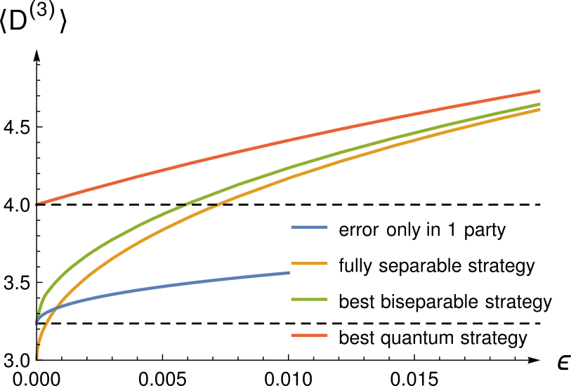
Figure A.4: Separable bounds for three-qubit W states. The figure shows the separable bound of the stabilizer witness $D^{(3)}$ defined in Eq. (E.1) with various assumptions of imprecision and separability. In blue we see the bound when assuming that the error is only present in one party, whereas in yellow we see the bound on fully separable strategies. The conjectured bound on biseparable strategies is shown in green and the quantum bound is shown in orange. The dashed black lines show the biseparable and quantum bound for no error in the measurements.

E.2 Stabilizer witness for 4-qubit cluster state

The expectation value of the operator

$$C^{(4)}= XZ\mathds{1}\mathds{1}+X\mathds{1}XZ+\mathds{1}ZXZ$$

$$+ZXZ\mathds{1}+\mathds{1}\mathds{1}ZX+ZX\mathds{1}X$$ (E.3)

is bounded by $\langle C^{(4)}\rangle\leq 4$ for biseparable states, whereas for the cluster state we have $\langle C^{(4)}\rangle=6$ [22]. This coincides both with the local bound and the algebraic maximum.

We now want to find the biseparable bound for imprecise measurements. Since this witness is linear, its maximal value is attained for a pure state. Assume that the first party is separable from the rest, such that our state has the form $|\psi\rangle=|\chi_{A}\rangle|\psi_{BCD}\rangle$. Since we are measuring in the $X-Z$ plane we set $|\chi(\theta)\rangle=\cos{\theta}|0\rangle+\sin{\theta}|1\rangle$ as before, resulting in the same expectation value as in Eq. (C.1)-(C.2). To find the optimal biseparable strategy we calculate the eigenvalue of

$$\langle\tilde{X}_{1}\rangle(\tilde{Z}_{2}\mathds{1}\mathds{1}+\mathds{1}\tilde{X}_{3}\tilde{Z}_{4})+\langle\tilde{Z}_{1}\rangle(\tilde{X}_{2}\tilde{Z}_{3}\mathds{1}+\tilde{X}_{2}\mathds{1}\tilde{X}_{4})$$

$$+\mathds{1}\tilde{Z}_{3}\tilde{X}_{4}+\tilde{Z}_{2}\tilde{X}_{3}\tilde{Z}_{4}.$$ (E.4)

and optimise over $\theta$. The result is shown in green in Fig. A.5).

Assuming errors in the measurements are only present in one party, the biseparable bound is the maximal eigenvalue of

$$\langle\tilde{X}_{1}\rangle(Z\mathds{1}\mathds{1}+\mathds{1}XZ)+\langle\tilde{Z}_{1}\rangle(XZ\mathds{1}+X\mathds{1}X)+\mathds{1}ZX+ZXZ,$$ (E.5)

optimised over $\theta$. This results in $2(1+\sqrt{1+4(1-2\epsilon)\sqrt{\epsilon(1-\epsilon)}})$ for $\theta=\pi/8$, shown in blue in Fig. A.5). The optimal fully separable strategy is obtained for the state $|\psi\rangle=|\chi(\theta)\rangle|\chi(\theta)\rangle|\chi(\theta)\rangle|\chi(\theta)\rangle$ and $\theta=\pi/8$, which results in the bound $1+2\sqrt{2}\sqrt{\epsilon(1-\epsilon)}+(1-2\epsilon)\big{(}4\sqrt{-(\epsilon-1)\epsilon}+3\sqrt{2}+2\sqrt{2}(1-2\epsilon)(2\epsilon+2\sqrt{-(\epsilon-1)\epsilon}-1)\big{)}$, shown in orange in Fig. A.5.

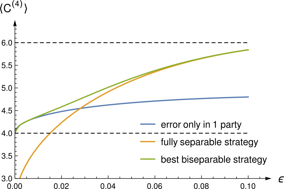
Figure A.5: Separable bounds for four-qubit cluster states. The figure shows the separable bound of the stabilizer witness $\mathcal{C}^{(4)}$ from Eq. (E.2) with various assumptions of imprecision and separability. The green line is the conjectured optimum. On the two extremes we have in blue the case where only the measurements in the party that is separated from the rest are altered, whereas in orange we have the bound for fully separable states. The quantum bound is shown in red, it is reached both by biseparable and fully separable states for high enough misalignments in the measurement direction. The dashed black lines show the biseparable and the quantum bound for accurate measurements.

Appendix F Noise tolerance and robustness analysis

The robustness of entanglement witnesses against various types of noise is an important property and relevant for experimental use. We compare the Mermin witness of Eq. (4) and the stabilizer witness of Eq. (7) with measurement imprecisions under two types of noise, namely white noise or depolarizing noise and dephasing noise on the state that is distributed. For the white noise we assume that the state that is actually measured is described by

$$\rho_{\text{iso}}(p)=p\outerproduct{GHZ}{GHZ}+\frac{1-p}{2^{n}}\mathds{1}.$$ (F.1)

In the case of dephasing noise, the state becomes

$$\rho_{\text{deph}}(p)= p\outerproduct{GHZ}{GHZ}+(1-p)\outerproduct{GHZ^{-}}{GHZ^{-}},$$ (F.2)

with $|GHZ^{-}\rangle=(|0\dots 0\rangle-|1\dots 1\rangle)\sqrt{2}$. To calculate the threshold level of noise where entanglement detection becomes impossible with a given inaccuracy $\varepsilon$ we have to distinguish two cases. First, we assume the best case scenario, where the measurements are precise. This corresponds to a situation where, although we expect a given imprecision in the measurements and thus correct the biseparable bound accordingly, the actual measurements are executed perfectly. Second, we assume the worst case, namely that the measurements are actually as imprecise as allowed by the fidelity bound.

For both cases, we can calculate the expectation value of the witnesses and compare it with the biseparable bounds. Assuming precise measurements, the expectation value of both witness-operators scales linearly with the level of depolarizing noise, $\tr(\mathcal{M}^{(4)}\rho_{\text{iso}}(p))=8p$ and $\tr(\mathcal{W}^{(4)}\rho_{\text{iso}}(p))=11p$. This means that the thresholds where entanglement detection becomes impossible are just the renormalised biseparable bounds $p=\mathbf{M}^{(4)}_{\text{bisep}}(\varepsilon)/8$ and $p=\mathbf{W}^{(4)}_{\text{bisep}}(\varepsilon)/11$, shown as a solid line in blue for the Mermin witness and in yellow for the stabilizer witness in Fig. A.6(a). Here the biseparable bound increases to account for imprecise measurements, but the expectation value of the witness remains the same since the actual measurements are performed perfectly. In case that the measurements can be imprecise, we find the lower bound $\tr(\mathcal{M}_{\varepsilon}^{(4)}\rho_{\text{iso}}(p))\geq 8p(1-8q^{2}+8q^{4})$ and $\tr(\mathcal{W}_{\varepsilon}^{(4)}\rho_{\text{iso}}(p))\geq p(3-24q^{2}+32q^{4})$ and with this $p=\mathbf{M}^{(4)}_{\text{bisep}}(\varepsilon)/(8(1-8q^{2}+8q^{4}))$ and $p=\mathbf{W}^{(4)}_{\text{bisep}}(\varepsilon)/(3-24q^{2}+32q^{4})$, shown as dashed lines in blue and yellow in Fig. A.6(b) respectively. Here we observe two effects: the separable bound increases to account for the imprecision in the measurements and the expectation value of the witness decreases due to this imprecision.

The analog calculation can be done for the dephasing noise model. For the best case scenario we compute $p=(\mathbf{M}^{(4)}_{\text{bisep}}(\varepsilon)-8)/16$ and $p=(\mathbf{W}^{(4)}_{\text{bisep}}(\varepsilon)-3)/8$ for the perfect measurements, shown as a solid line in blue for the Mermin witness and in orange for the stabilizer witness in Fig. A.6(b). For the worst case we have $p=\mathbf{M}^{(4)}_{\text{bisep}}(\varepsilon)/(16(1-8q^{2}+8q^{4}))+1/2$ and $p=(\mathbf{W}^{(4)}_{\text{bisep}}(\varepsilon)+3(1-12q^{2}+10q^{4}))/(2(3-30q^{2}+31q^{4}))$ for the most imprecise measurements, shown as a dashed lines in Fig. A.6(b).

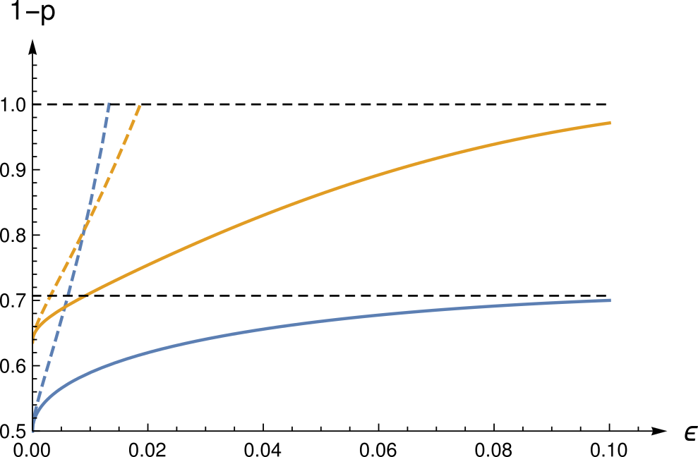
(a)

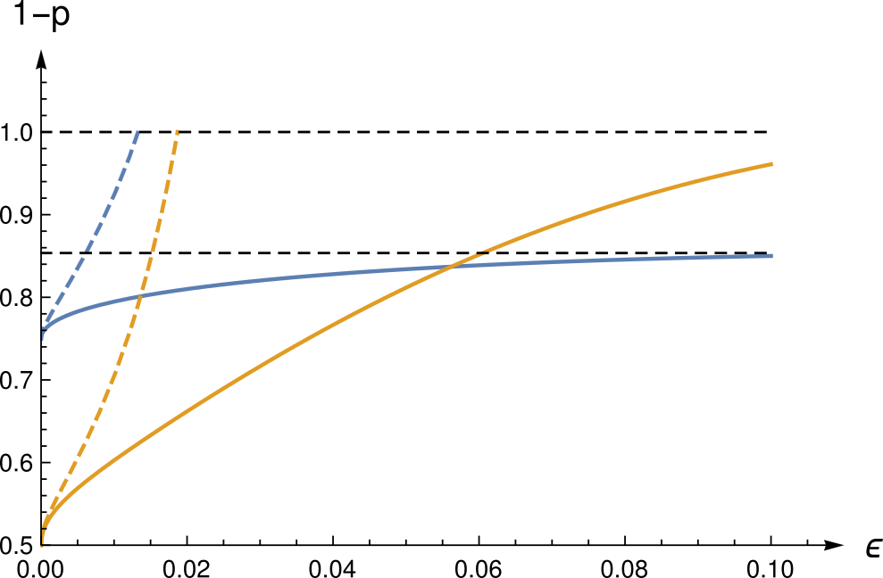
(b)

Figure A.6: Comparison of the robustness under noise. The plot shows $p$, where $1-p$ is the maximally tolerated noise level, versus the bound $\varepsilon$ on the misalignment of the measurements for the Mermin witness (blue) and the stabilizer witness (yellow) under white noise (above) and dephasing noise (below). The solid line shows the minimal value of $p$ that is needed to detect entanglement under the assumption of imprecise measurements, but where actually perfect measurements are performed. The dashed line shows the minimal value of $p$ that is needed to detect entanglement under the same assumption, with the worst possible measurements constraint to this assumption. These two lines mark two extreme cases, realistically the visibility lies somewhere between them.

We see that, depending on the type of noise we encounter, one witness is more resistant than the other. This behaviour changes with increasing imprecision in the performed measurements. Noteworthy is that the Mermin witness loses less noise tolerance with increasing imprecision, when the potential imprecision of the measurements is included in the analysis but actual perfect measurements are performed. That is, while for both witnesses the visibility decreases, this rate is lower for the Mermin witness. In the case of dephasing noise, this is more evident: initially, the Mermin witness has a lower visibility, but with increasing imprecision, this changes and the visibility becomes higher than for the stabilizer witness. This makes sense since for the Mermin witness there is a gap between the quantum bound and the bilocal bound. Therefore the witness is more robust against misalignments in the measurement direction, even assuming a high inaccuracy does still allow for potential entanglement detection. In the case of actually imprecise measurements, the visibility drops sharply for both witnesses and types of noise, here we see no clear advantage for either witness.

References

- Gühne and Tóth [2009] O. Gühne and G. Tóth, Entanglement detection, Physics Reports 474, 1 (2009).
- Horodecki et al. [2009] R. Horodecki, P. Horodecki, M. Horodecki, and K. Horodecki, Quantum entanglement, Rev. Mod. Phys. 81, 865 (2009).
- Friis et al. [2019] N. Friis, G. Vitagliano, M. Malik, and M. Huber, Entanglement certification from theory to experiment, Nature Reviews Physics 1, 72 (2019).
- Horodecki et al. [1996] M. Horodecki, P. Horodecki, and R. Horodecki, Separability of mixed states: necessary and sufficient conditions, Physics Letters A 223, 1 (1996).
- Terhal [2000] B. M. Terhal, Bell inequalities and the separability criterion, Physics Letters A 271, 319 (2000).
- Lewenstein et al. [2000] M. Lewenstein, B. Kraus, J. I. Cirac, and P. Horodecki, Optimization of entanglement witnesses, Phys. Rev. A 62, 052310 (2000).
- Horodecki et al. [2006] M. Horodecki, P. Horodecki, and R. Horodecki, Separability of mixed quantum states: linear contractions approach, Open Systems & Information Dynamics 10.1007/s11080-006-7271-8 (2006), arXiv:quant-ph/0206008 [quant-ph] .
- Seevinck and Uffink [2007] M. Seevinck and J. Uffink, Local commutativity versus bell inequality violation for entangled states and versus non-violation for separable states, Phys. Rev. A 76, 042105 (2007).
- Rosset et al. [2012] D. Rosset, R. Ferretti-Schöbitz, J.-D. Bancal, N. Gisin, and Y.-C. Liang, Imperfect measurement settings: Implications for quantum state tomography and entanglement witnesses, Phys. Rev. A 86, 062325 (2012).
- Morelli et al. [2022] S. Morelli, H. Yamasaki, M. Huber, and A. Tavakoli, Entanglement detection with imprecise measurements, Phys. Rev. Lett. 128, 250501 (2022).
- Bancal et al. [2011] J.-D. Bancal, N. Gisin, Y.-C. Liang, and S. Pironio, Device-independent witnesses of genuine multipartite entanglement, Phys. Rev. Lett. 106, 250404 (2011).
- Moroder et al. [2013] T. Moroder, J.-D. Bancal, Y.-C. Liang, M. Hofmann, and O. Gühne, Device-independent entanglement quantification and related applications, Phys. Rev. Lett. 111, 030501 (2013).
- Barreiro et al. [2013] J. T. Barreiro, J.-D. Bancal, P. Schindler, D. Nigg, M. Hennrich, T. Monz, N. Gisin, and R. Blatt, Demonstration of genuine multipartite entanglement with device-independent witnesses, Nature Physics 9, 559 (2013).
- Pan et al. [2000] J.-W. Pan, D. Bouwmeester, M. Daniell, H. Weinfurter, and A. Zeilinger, Experimental test of quantum nonlocality in three-photon greenberger–horne–zeilinger entanglement, Nature 403, 515 (2000).
- Bouwmeester et al. [1999] D. Bouwmeester, J.-W. Pan, M. Daniell, H. Weinfurter, and A. Zeilinger, Observation of three-photon greenberger-horne-zeilinger entanglement, Phys. Rev. Lett. 82, 1345 (1999).
- Gottesman and Chuang [1999] D. Gottesman and I. L. Chuang, Demonstrating the viability of universal quantum computation using teleportation and single-qubit operations, Nature 402, 390 (1999).
- Mermin [1990] N. D. Mermin, Extreme quantum entanglement in a superposition of macroscopically distinct states, Phys. Rev. Lett. 65, 1838 (1990).
- Gisin and Bechmann-Pasquinucci [1998] N. Gisin and H. Bechmann-Pasquinucci, Bell inequality, Bell states and maximally entangled states for n qubits, Physics Letters A 246, 1 (1998).
- Werner and Wolf [2000] R. F. Werner and M. M. Wolf, Bell’s inequalities for states with positive partial transpose, Phys. Rev. A 61, 062102 (2000).
- Liang et al. [2014] Y.-C. Liang, F. J. Curchod, J. Bowles, and N. Gisin, Anonymous quantum nonlocality, Phys. Rev. Lett. 113, 130401 (2014).
- Tóth and Gühne [2005] G. Tóth and O. Gühne, Detecting genuine multipartite entanglement with two local measurements, Phys. Rev. Lett. 94, 060501 (2005).
- Tóth and Gühne [2005] G. Tóth and O. Gühne, Entanglement detection in the stabilizer formalism, Physical Review A 72 (2005).
- Briegel and Raussendorf [2001] H. J. Briegel and R. Raussendorf, Persistent Entanglement in Arrays of Interacting Particles, Phys. Rev. Lett. 86, 910 (2001).
- Tavakoli [2023] A. Tavakoli, Quantum steering with imprecise measurements (2023), arXiv:2308.15356 [quant-ph] .
- Zhang et al. [2015] C. Zhang, Y.-F. Huang, Z. Wang, B.-H. Liu, C.-F. Li, and G.-C. Guo, Experimental greenberger-horne-zeilinger-type six-photon quantum nonlocality, Phys. Rev. Lett. 115, 260402 (2015).
- Cao et al. [2022] H. Cao, M.-O. Renou, C. Zhang, G. Massé, X. Coiteux-Roy, B.-H. Liu, Y.-F. Huang, C.-F. Li, G.-C. Guo, and E. Wolfe, Experimental demonstration that no tripartite-nonlocal causal theory explains nature’s correlations, Phys. Rev. Lett. 129, 150402 (2022).
- Bancal et al. [2012] J.-D. Bancal, C. Branciard, N. Brunner, N. Gisin, and Y.-C. Liang, A framework for the study of symmetric full-correlation bell-like inequalities, Journal of Physics A: Mathematical and Theoretical 45, 125301 (2012).
- Wang et al. [2016] Y. Wang, A. Kumar, T.-Y. Wu, and D. S. Weiss, Single-qubit gates based on targeted phase shifts in a 3d neutral atom array, Science 352, 1562 (2016).
- Debnath et al. [2016] S. Debnath, N. M. Linke, C. Figgatt, K. A. Landsman, K. Wright, and C. Monroe, Demonstration of a small programmable quantum computer with atomic qubits, Nature 536, 63 (2016).
- Fang et al. [2022] C. Fang, Y. Wang, S. Huang, K. R. Brown, and J. Kim, Crosstalk suppression in individually addressed two-qubit gates in a trapped-ion quantum computer, Phys. Rev. Lett. 129, 240504 (2022).
- Cao et al. [2023] S. Cao, B. Wu, F. Chen, M. Gong, Y. Wu, Y. Ye, C. Zha, H. Qian, C. Ying, S. Guo, et al., Generation of genuine entanglement up to 51 superconducting qubits, Nature , 1 (2023).
- Córcoles et al. [2015] A. D. Córcoles, E. Magesan, S. J. Srinivasan, A. W. Cross, M. Steffen, J. M. Gambetta, and J. M. Chow, Demonstration of a quantum error detection code using a square lattice of four superconducting qubits, Nature communications 6, 6979 (2015).
- Ansmann et al. [2009] M. Ansmann, H. Wang, R. C. Bialczak, M. Hofheinz, E. Lucero, M. Neeley, A. D. O’Connell, D. Sank, M. Weides, J. Wenner, et al., Violation of bell’s inequality in josephson phase qubits, Nature 461, 504 (2009).
- Bent et al. [2015] N. Bent, H. Qassim, A. A. Tahir, D. Sych, G. Leuchs, L. L. Sánchez-Soto, E. Karimi, and R. W. Boyd, Experimental realization of quantum tomography of photonic qudits via symmetric informationally complete positive operator-valued measures, Phys. Rev. X 5, 041006 (2015).
- Mirhosseini et al. [2013] M. Mirhosseini, M. Malik, Z. Shi, and R. W. Boyd, Efficient separation of the orbital angular momentum eigenstates of light, Nature communications 4, 2781 (2013).
- Uffink [2002] J. Uffink, Quadratic bell inequalities as tests for multipartite entanglement, Phys. Rev. Lett. 88, 230406 (2002).