Mixture distributions for probabilistic forecasts of disease outbreaks

Abstract

Collaboration among multiple teams has played a major role in probabilistic forecasting events of influenza outbreaks, the COVID-19 pandemic, other disease outbreaks, and in many other fields. When collecting forecasts from individual teams, ensuring that each team’s model represents forecast uncertainty according to the same format allows for direct comparison of forecasts as well as methods of constructing multi-model ensemble forecasts. This paper outlines several common probabilistic forecast representation formats including parametric distributions, sample distributions, bin distributions, and quantiles and compares their use in the context of collaborative projects. We propose the use of a discrete mixture distribution format in collaborative forecasting in place of other formats. The flexibility in distribution shape, the ease for scoring and building ensemble models, and the reasonably low level of computer storage required to store such a forecast make the discrete mixture distribution an attractive alternative to the other representation formats.

Keywords Ensemble modeling  $\cdot$ Proper scoring rules  $\cdot$ Influenza outbreaks  $\cdot$ COVID-19

1 Introduction

Predicting the outcomes of prospective events is the object of much scientific inquiry and the basis for many decisions both public and private. Because predictions of the future can never be precise, it is usually desirable that a level of uncertainty be attached to any prediction. In recent years, it has become increasingly desirable that forecasts be probabilistic in order to account for uncertainty in predicted quantities or events [1]. Weather forecasting [2], economics [3], and disease outbreaks [4] are some of the areas where probabilistic forecasting is used.

A probabilistic forecast is a forecast in which possible outcomes are assigned probabilities. There are a number of ways whereby probabilities or uncertainty may be represented. A common representation is either a continuous or discrete parametric distribution, given as a probability density/mass function. Much of the literature on calibration, sharpness, and scoring of a forecast pertains to parametric distribution forecasts [5, 6, 2]. Other common representations include samples [7], discretized bin distributions [8], and quantile forecasts [9, 10]. Each representation may be more or less appropriate than the others for a given problem, but knowing how to interpret, score, and construct ensemble forecasts for a selected representation is essential when multiple teams collaborate in the same forecasting project.

Two collaborative projects on forecasting disease outbreaks for which many separate forecasts are used include the United States Centers for Disease Control (CDC) annual competition for forecasting the influenza outbreak [11] and the COVID-19 Forecast Hub which has continuously operated since the start of the COVID-19 pandemic in the US in early 2020 [12].

1.1 CDC flu forecasting

During the 2013-14 flu season, the CDC began hosting an annual competition for forecasting the timing, peak, and intensity of the year’s flu season. The specific events to be forecast were known as targets. Forecasts for these different targets included forecasts for one, two, three, and four weeks into the future. National flu data was provided weekly to academic teams not directly affiliated with the CDC who used that data to construct forecasts using whatever methods they chose. Historically, the forecasts were submitted in a discretized bin distribution or a bin distribution format. A bin distribution is a probability distribution represented by breaking the numeric range of an outcome into intervals or bins and directly assigning to each bin the probability that the event falls within the bin. During previous flu seasons the binning scheme or the assignment of bin values was on a numeric scale with a bounded range, and the prediction of a specific target was a set of probabilities assigned to each bin [8]. These forecasts were then evaluated against actual flu activity, and at the end of the season a winning team was declared [11]. The CDC continues to host a flu forecasting project, but since the 2021-22 season the only target for forecasts has weekly hospitalizations and the forecast submission format has been quantile forecasts similar to those described in the following section.

Flu forecasting has provided the CDC, competing teams, and other interested parties a chance to collaborate and improve their forecasting from season to season. One proposed way to enhance prediction has been to aggregate the various teams’ forecasts into a multi-model ensemble forecast [8, 13, 14], or an ensemble forecast. An ensemble forecast is a combination of several component forecast models into one model which often yields better predicting power than the individual models [15]. Such an ensemble made from multiple influenza competition forecasts did in fact outperform the individual component models [14].

1.2 COVID-19 Forecast Hub

In March 2020, at the onset of the COVID-19 pandemic, the United States COVID-19 Forecast Hub was founded. Borrowing from the work done in the CDC flu competition, the COVID-19 Forecast Hub was a central site in which dozens of academic teams collaborated to forecast the ongoing COVID-19 pandemic. Every week relevant pandemic data aws provided to these teams who constructed forecast models to predict the target cases, hospitalizations, and deaths due to COVID-19. Forecasts were made on the US county, state, and national levels and for days, weeks, and months ahead. These forecasts were aggregated into a single ensemble forecast. The model data, forecasts, and the ensemble forecast were passed along to the CDC for its use in official communication [12]. Figure 1 is from an official CDC report from August 2021. It shows forecasts from the COVID-19 Forecast Hub of increment deaths and cumulative deaths due to COVID-19.

Though similar to the forecasting in the CDC flu competition, the format of the COVID-19 Forecast Hub has key distinctions. First, this project has been operating continuously since it began, so forecasts have been made for over 100 straight weeks. Second, rather than bin distributions the forecasts are requested as the predictive median and predictive intervals for various nominal levels depending on the target to be predicted [10]. Each value in a predictive interval is a value for a quantile at a specified nominal level. This makes a set of predictive intervals a quantile forecast or a forecast made up of a set of quantiles and corresponding values. Collecting forecasts as quantile forecasts instead of bin forecasts brings with it differences in how to score the forecasts, construct an ensemble forecast, and store the forecasts among other differences. Ray et. al show that ensemble forecasts in the COVID-19 Forecast Hub provide precise short-term forecasts which decline in accuracy in longer term forecasts approaching four weeks [16].

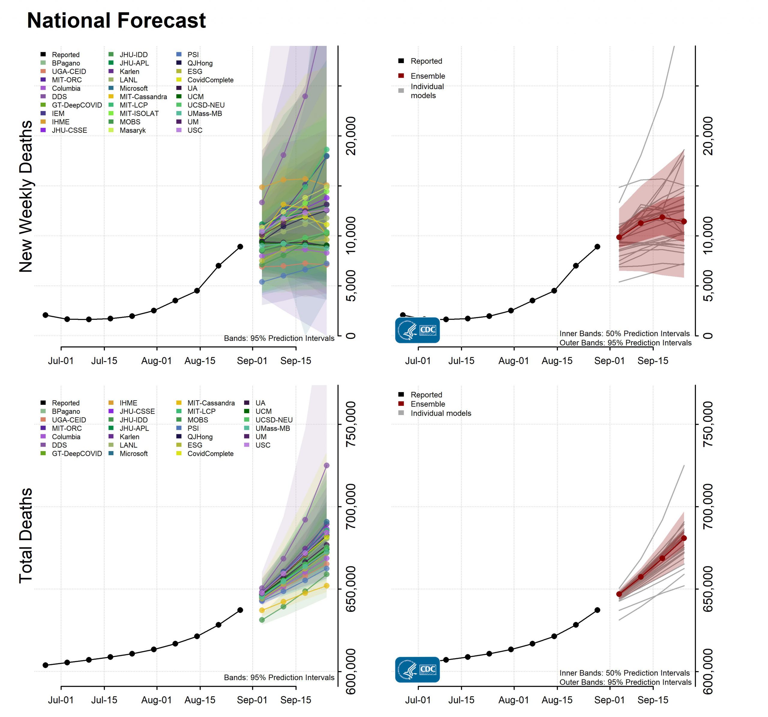
Figure 1: This image, published on www.cdc.gov in August 2021 as official public communication by the CDC, shows forecast models for national new weekly deaths due to COVID-19 in the top row and cumulative deaths on the bottom row. The plots in the left column show prediction intervals from multiple teams whereas the plots on the right show the intervals for an ensemble forecast model with gray lines that are individual model point forecast predictions.

1.3 Outline

In the context of collaborative forecasting like that of the CDC flu competition or the COVID-19 Forecast Hub, bin forecasts and quantile forecasts have become important representations. Yet both representations come with their drawbacks. Computer storage for instance might be a concern if many bin distributions are used for forecasting, and scoring methods are limited if forecasts are quantile forecasts. In this paper, we propose the use of finite mixture distributions as a means of forecasting for collaborative projects similar to the CDC flu competition or the COVID-19 Forecast Hub. A finite mixture distribution –which we will refer to as a mixture distribution– is a distribution constructed by aggregating a finite collection of other distributions. In this paper, we focus on the case where the collection of distributions are parametric distributions. In Section 2, popular probabilistic forecast representations are defined and reviewed. For each representation, we review methods of scoring, storing, constructing ensembles, and other aspects. Section 3 presents using mixture distributions in a collaborative forecast project and discusses tools for scoring and constructing an ensemble forecast. Section 4 is a retrospective study of the CDC flu competition and COVID-19 Forecast Hub forecasts and an attempt to assess whether forecast models may be approximated by one component mixture distributions.

2 Probabilistic forecast representations

At least four forecast representations are commonplace in forecasting. In a collaborative setting, certain aspects of each representation should be considered including scoring, computer storage, and how to construct an ensemble forecast. For each representation discussed herein, applications of each of those aspects are also discussed.

2.1 Things to consider in collaborative projects

In this section we introduce three topics which ought to be considered in a collaborative forecast project including forecast scoring, computer storage of forecasts, and ensemble forecast construction from multiple models.

2.1.1 Scoring

Scoring rules are used to numerically evaluate or score a probability forecast. The score is a measure of the accuracy of the forecast and where multiple forecasts exist the score for each may be used to compare forecasts. If a scoring rule is proper, then the best possible score is obtained by reporting the true distribution. The rule is strictly proper if the best score is unique. Under proper scoring rules, a forecaster has no incentive to be dishonest in their submission [17]. This makes proper scoring rules ideal for evaluating forecasts. We will limit our review of scoring methods to rules which are proper.

2.1.2 Storage

For a collaborative forecast project where many researchers are involved and many predictions are collected, computer storage may need to be addressed. As an example of required computer storage, the repository for the COVID-19 Forecast Hub contained 85 million forecasts as of April 4, 2022 which required more than 11.7 gigabytes of storage. [18]. When determining the goals of a forecast project, there should be consideration of the storage required for different forecast representations.

2.1.3 Ensemble model

An ensemble model is a statistical model made by combining information from two or more individual statistical models. Private and public decisions are regularly made after combining information from multiple sources. For a given problem, information from one source may provide insight on a subject which other sources fail to capture. Likewise one statistical model may provide insight that another model does not. Thus when multiple models are combined, the resulting ensemble may outperform the individual models.

As probabilistic forecasting becomes more commonplace, so too does ensemble modeling. Ensembles have been used extensively in weather and climate modeling [2], and they have been used increasingly in modeling infectious disease outbreaks [4]. Ensembles allow for an incorporation of multiple signals –often from differing data sources– and sometimes individual model biases are canceled out or reduced by biases from other models [14, see references therein]. In several disease outbreak studies, ensemble forecasts have been shown to outperform individual model forecasts [16, 15, see references therein]. Construction of an ensemble may be done by combining individual forecast models using weighted averages. This has been called stacking [19] or weighted density ensembles [20].

Considered the state-of-the-art techniques for combining component distributions into an ensemble distribution are nonhomogeneous regression and ensemble model averaging (MA), both of which are defined by Gneiting and Katzfuss [1]. In the context of an ensemble made from component models submitted from various sources, MA may be preferable because it does not require that modeling methods for individual components be the same. The general form for an MA ensemble distribution $p^{E}$ is defined in equation (1), where $p_{m}$ is the $m^{th}$ component forecast distribution and $0\leq w_{m}\leq 1$ is a weight assigned to that component where $\sum_{m}w_{m}=1$.

$$p^{E}(x)=\sum_{m=1}^{M}w_{m}p_{m}(x)$$ (1)

In MA, the final model does not have to be specified beforehand and the resulting forecast will be a mixture distribution of all component forecasts. Many methods exist for estimating weights. Some of these methods include maximum likelihood estimation [21], Markov chain Monte Carlo (MCMC) sampling [22], Bayesian model averaging, Akaike or AIC weights, [23], minimizing the CRPS of the ensemble [2], and others.

2.2 Probabilistic forecast representations

Probabilistic forecast uncertainty can take on many representations. In this section we describe parametric distributions, sample distributions, bin distributions, and predictive intervals as representation forecasts. Following the description of these four representations, mixture distributions are introduced.

2.2.1 Parametric distributions

A parametric distribution is a discrete or continuous probability distribution described by a known function $p(x):=p(x|\theta)$. The function $p(x)$ is called a probability mass function (pmf) if the distribution is discrete and a probability density function (pdf) if the distribution is continuous. Here $\theta$ is a vector of parameters contained in the parameter space of the distribution.

For a forecast represented as a parametric distribution with pmf/pdf $p_{m}(\cdot)$, the accuracy of the forecast may be measured by how likely the realized value $x^{*}$ is to occur. Commonly used proper scoring rules for parametric distributions include the logarithmic score (LogS), the continuous rank probability score (CRPS) [24] [25], and the interval/Brier score (IS) [17] among others. See also [1] Section 3 for more on proper scoring functions. The definitions (2), (3), and (11) are found in the review by Krueger. For a forecast with pdf/pmf $p(\cdot)$, (2) evaluates the probability of the observed value $x^{*}$.

$$\text{LogS}(p,x^{*})=-\log p(x^{*})$$ (2)

The goal for a forecaster is to minimize the LogS, so a forecast $p^{\prime}(x^{*})$ is considered superior to $p(x^{*})$ if $\text{LogS}(p^{\prime},x^{*})<\text{LogS}(p,x^{*})$. The LogS is limited to scoring forecasts with density functions and evaluating those densities only at the point $x^{*}$. For the cumulative distribution (CDF) $F$ of a parametric distribution, the CRPS is defined in (3). Here too a smaller score indicates a more accurate forecast.

$$\text{CRPS}(F,x^{*})=\int_{-\infty}^{\infty}(F(x)-1_{\{x*\leq x\}})^{2}dx$$ (3)

Standard practice for constructing an ensemble model from multiple parametric models is to use MA. For selecting distribution weights for the ensemble, minimizing the LogS or CRPS of $p^{E}(x)$ is common. Because it is evaluated over the whole distribution, minimizing the CRPS has some nice properties, but it can also be difficult to compute. For example, when the forecast is a mixture of a truncated normal distribution (TN) and a truncated lognormal (TL), the CRPS is not available in closed form [2].

Generally computation and evaluation of parametric distribution functions is easy. For most commonly used parametric distributions –normal, lognormal, Poisson, gamma, etc.– there is software readily available to compute density, distribution, and quantile values. A completely defined continuous parametric distribution may be evaluated at a continuously infinite number of values which we call an infinite resolution. Requirements for storage are also low compared to other representations that will be discussed since the most common parametric distributions can be fully defined with three or four pieces of information including the distribution family and the corresponding parameters. Table 1 contains enough information to completely define a Lognormal(1,0.4) truncated to the inteval $[0,8]$. The truncation is done here so as to make a direct comparison with the distributions shown later in Tables 2 and 3.

Table 1: This is an example of information required to specify a truncated lognormal distribution.

family	param1	param2	lowerlim	upperlim
lnorm	1	0.4	0	8

A drawback of representing a forecast in a parametric distribution is the lack of flexibility in the model selection. Easy computation and evaluation of these models is limited to what is available in software, so certain distributional shapes may be unattainable. Requiring a parametric forecast also bars the use of some statistical methods which might be used to create a forecast model including some Bayesian methods where a posterior distribution cannot be computed in closed form.

2.2.2 Sample distributions

Forecasters may want more flexibility in modeling than a parametric distribution can provide. Methods that require sampling from a posterior distribution or bootstrap sampling to obtain a forecast distribution are examples where parametric distributions may not be appropriate for modeling because of the lack of flexibility in distribution shape.

A sample distribution is composed of a collection of, possibly weighted, random variables $(X_{1},...,X_{n})$ where $X_{i}\sim D$ and $D$ is some distribution. From this sample, statistics such as mean, median, variance, and quantiles may be calculated. An empirical cumulative distribution function (ECDF) may also be calculated as in (4). If a sufficiently large sample is generated from a distribution for which an expectation exists, the sample will closely approximate the true distribution.

$$\text{ECDF}=F_{n}(x)=\frac{1}{n}\sum_{i=1}^{n}\mathbb{I}(X_{i}\leq x)$$ (4)

For common distribution families it is easy to generate large samples using existing functions in R and other programming platforms. For some distributions for which the mathematical formula is unknown or is not in closed form, more sophisticated methods may be required to generate samples. Bayesian analyses may require MCMC sampling to generate a sample. Such samples are useful in that the true distribution may be closely approximated without knowing the true mathematical form.

Under the sample distribution representation, the options that a researcher has for constructing a forecast are more than if they are asked to submit a parametric distribution, and the range of possible shapes for a distribution is larger. In the last few decades, increased computing power and improvements in MCMC sampling have greatly contributed to growth in the use of sample distributions for forecasting [17] [7, see examples listed therein].

To properly score a forecast represented by a sample distribution, both the CRPS and LogS may be used. The CRPS has the advantage here of scoring the sample distribution directly since the CDF in (3) may be replaced with the ECDF in (4). To use the LogS to score a forecast, a density function for the sample may be approximated. Common approximations include a kernel density (KD) or Gaussian approximation (GA) [7, for example].

The KD in (5) is defined by Krueger et. al where $K$ is a kernel function, and $h_{n}$ is a suitable bandwidth. The GA is defined in (6) where $\Phi$ is the standard normal CDF and $\hat{\mu}_{n}$ and $\hat{\sigma}_{n}$ are the empirical mean and standard deviation of the sample $(X_{i})$ [7, see also for a comparison of scoring MCMC drawn forecasts between the CRPS and the LogS].

$$\hat{p}_{n}^{KD}(x)=\frac{1}{nh_{n}}\sum_{i=1}^{n}K\left(\frac{x-X_{i}}{h_{n}}\right)$$ (5)

$$\hat{F}_{n}^{GA}(x)=\Phi\left(\frac{x-\hat{\mu}_{n}}{\hat{\sigma}_{n}}\right)$$ (6)

To build an ensemble model from sample distribution forecasts, the MA construction from (1) may be used only replacing $p_{m}$ with the approximate KD or GA pdf functions -$\hat{p}_{n_{m}}^{KD}$ or $\hat{p}_{n_{m}}^{GA}$ respectively where $\hat{p}_{n}^{GA}$ is the pdf corresponding to (6). The optimal weights $w_{m}$ may be estimated by maximizing the likelihood or minimizing the CRPS. If the desire is that the ensemble has uniform weights, a random sample from $(X_{n})_{m}$ with probability $w_{m}$ can be obtained.

A potentially large issue with using sample distributions is the amount of storage it may require. For example when making MCMC draws from a posterior distribution, the final sample distribution can have a sample size of thousands or tens of thousands. Maybe not all distributions would require such a large sample size, but sizes of at least dozens or hundreds would be required for each forecast prediction. For any project the size of the CDC flu competition or the COVID-19 Forecast Hub, the storage required would be large and potentially expensive.

2.2.3 Bin distributions

An alternative to parametric distributions and sample distributions, which allows for higher flexibility in distribution shape than a parametric distribution and will usually require less storage space than samples is the bin distribution. A bin distribution may be constructed over a set $A=[a,b)$ by partitioning $A$ into a set of $K$ bins $\{B_{i}\}_{i=1}^{K}$ where $B_{i}=[b_{i-1},b_{i})$ and $\cup_{i=1}^{K}B_{i}=A$. Based on the problem to be forecast, researchers will determine the possible range $A$ and select the number of bins and the sizes for each bin. It may be the case that a collaborative project will set the widths of all bins to be equal so that $\Delta=b_{i}-b_{i-1}$ is the same width for all $i$ [8]. To complete the construction, a probability $p_{i}$ is assigned to each $B_{i}$ where $\sum p_{i}=1$. These probabilities are determined by the forecasters. This representation with a given bin and assigned probability may be treated like a discrete distribution with a pmf in that the calculation of the cumulative distribution is done similarly to that of a discrete parametric distribution. The cumulative distribution may be calculated as in (7). Here $p_{i}$ is the probability for the bin $B_{i}$ where $x\in B_{i}$.

$$P(X\leq x)=\sum_{i=1}^{n:x\in B_{n}}p_{i}$$ (7)

If the value to be forecast takes on discrete values, a common discrete distribution, such as a Bernoulli or Poisson distribution, may sometimes be used to assign probabilities to each of the bins. When the values to be forecast are continuous, a forecaster may need to employ a method of discretization to a forecast distribution. There are a number of possible ways to do this including those outlined by Chakraborty and Subrata [26].

For the first several seasons when the CDC hosted the flu competition, the forecast representation used was the bin distribution. The CDC has also used the bin distribution represetation for other disease outbreak forecast projects. In that context it has become the standard representation [27]. Much work has been done in evaluating and constructing ensemble models on influenza forecasts represented by discretized bins [8, 13, 28].

Because a bin distribution can be viewed as a pmf, methods for proper scoring already discussed –LogS and CRPS– are useable and MA is a valid method for ensemble construction. Reich et. al used MA to combine multiple forecasts from the flu competition. They constructed and compared ensemble models with different weighting schemes including equally weighted components, $w_{m}=1/M$, and estimating weights according to the model specification. To estimate weights they used the expectation maximization (EM) algorithm [14, see supplementary material within for details].

The exact amount of information required for a bin forecast will vary depending on the permitted range of the forecast and the desired resolution. In the CDC flu contest, a forecast might have 131 bins between 0% and 13% –bins having increments of 0.1 or 0.01%– with corresponding probabilities in each. This makes 262 pieces of information per prediction. For any binning scheme of more than two or three bins, the information requirement for a bin distribution will be higher than for a parametric distribution. Table 2 illustrates what the bin distribution discretized from a Lognormal(1,0.4) distribution truncated over $[0,8]$ looks like in 41 equally spaced bins. The discretization was done such that the probabilities $p_{i}$ are calculated as in (8) where $p^{TL}$ is the pdf of a truncated Lognormal(1,0.4). This is similar to Methodology-IV from Chakraborty [26, 29]. The truncation here is done because in practice a bin forecast will generally have a finite support.

$$p_{i}=\int_{b_{i-1}}^{b_{i}}p^{TL}(x)dx$$ (8)

Submitted as a forecast prediction, the distribution illustrated in Table 2 includes 82 values. For parts of the CDC influenza competition some forecasts included up to 262. This is far less storage than the possible thousands of draws from a sample distribution but is still much larger than the three or five pieces of information required to report a lognormal or truncated lognormal distribution.

Table 2: This is a storage example of a discretized lognormal with $\mu=1$ and $\sigma=0.4$ truncated over $[0,8]$.

bin	prob
…	…
[1.4, 1.6)	0.04414
[1.6, 1.8)	0.05896
[1.8, 2.0)	0.07032
[2.0, 2.2)	0.07172
[2.2, 2.4)	0.07955
…	…

Besides the potentially large amount of information required per forecast, creating the right binning scheme may be a challenge. Because there must be a finite number of bins, forecast distributions often have finite support. And where the range of possible outcomes to a problem is not well known, the right binning scheme may be hard to produce. This may depend on the details of the event to be forecast, but in the case of the COVID-19 outbreak, choosing the right set of bins posed a few problems.

2.2.4 Interval forecasts

When deciding how forecasts should be represented in the COVID-19 Forecast Hub, the time pressure of generating forecasts and the large range for possible outcomes both contributed to the COVID-19 Forecast Hub decision to forego trying to create the right binning scheme and use quantile forecasts to forecast the COVID-19 pandemic [10]. The COVID-19 Forecast Hub requires predictions to be submitted as 11 or three nominal intervals –depending on the specific target and unit to be forecast– and a median. Likewise the CDC flu forecasting project has used this same format for the past two seasons [30].

A quantile forecast is constructed as in (9). Here for $N$ given quantile levels $\alpha_{1},...,\alpha_{N}$; $q_{1},...,q_{N}$ are the values such that we have (9). When the quantiles are reported as prediction intervals we have (10).

$$P(Y\leq q_{1})=\alpha_{1},P(Y\leq q_{2})=\alpha_{2},...,P(Y\leq q_{N})=\alpha_{N}$$ (9)

$$P(Y\leq q_{1})=\alpha_{1},P(Y\leq q_{2})=\alpha_{2},...,P(Y\leq q_{N-1})=1-\alpha_{2},P(Y\leq q_{N})=1-\alpha_{1}$$ (10)

The CRPS and LogS may not be used to score a quantile forecast, and MA may not be used for constructing an ensemble from multiple quantile forecasts. Methods for scoring quantile forecasts and constructing ensemble forecasts are limited, and when given only in quantiles the shape of a distribution is not known. In fact nothing is known about the tails or the uncertainty beyond the most extreme reported quantile values. In the COVID-19 Forecast Hub forecasts, nothing is reported about the range below the $1^{st}$ quantile or above the $99^{th}$. Yet the quantile representation has its advantages. Quantile forecasts allow for forecasters to submit fairly detailed forecasts without restricting the range of possible values. Since quantiles are easily calculated from any regular distribution type –using the quantile function for parametric functions or calculating sample quantiles– we consider quantile forecasts to be highly flexible in terms of what methods forecasters may employ in modeling.

To score a quantile forecast, neither the LogS nor the CRPS may be used, but another proper scoring rule the IS may be used. For an observed outcome $x^{*}$ and a prediction interval $(l,r)$ where $l$ and $r$ are the $\alpha/2$ and $(1-\alpha/2)$ quantiles that bound the central $(1-\alpha)$ prediction interval, the IS is defined as in (11). This is a sum –weighted by $\alpha$– of the width of the interval and the distance between $x^{*}$ and the interval (if $x^{*}$ is not captured in the interval) [1]. The IS requires only a single central $(1-\alpha)\times 100$ prediction interval.

$$IS_{\alpha}(l,r;x^{*})=(r-l)+\frac{2}{\alpha}(l-x^{*})1\{x^{*}<l\}+\frac{2}{\alpha}(x^{*}-r)1\{x^{*}>r\}$$ (11)

When a quantile forecast is made up of multiple intervals each with different $\alpha$ levels, the weighted interval score (WIS) may be used. Bracher et. al use the WIS to score COVID-19 quantile forecasts [10]. There are multiple versions of the WIS, some of which are described in Bracher et. al, but the version used by the COVID-19 Forecast Hub for a forecast of $K$ intervals is defined in (12). Here $median$ refers to the predictive median and $w_{k}=\alpha_{k}/2$ is the weight on the $k^{th}$ interval. With that selection of weights, it may be shown that the WIS approximates the CRPS [10, see S1 Text therein].

$$WIS_{0,K}(F_{m},x^{*})=\frac{1}{K+1/2}\left(w_{0}|x^{*}-median|+\sum_{k=1}^{K}\{w_{k}IS_{\alpha_{k}}(F_{m},x^{*})\}\right)$$ (12)

Bogner, Liechti, and Zappa compared scoring forecasts of quantiles with the Quantile Score (QS) similar to the interval score and scoring distribution functions fit to those quantiles using the CRPS [31]. The CRPS corresponds to the integral of the QS over all possible thresholds rather than just specific quantiles, so it more effectively reveals deficiencies in parts of the distribution and especially in the tails past the end points of quantiles used in QS or IS. Thus there may be something lost in terms of scoring when the WIS is used since it also is constructed from the IS.

Like the CRPS, not only does the WIS provide an easily interpretable proper score for interval forecasts, but it may also be useful when building an ensemble forecast. The ensemble forecast constructed by the COVID-19 Forecast Hub is made as an equally-weighted average of forecasts from the component models. More specifically, each quantile value of the ensemble is the average of values from all models corresponding to the same quantile [16]. For $M$ models each with $K$ quantiles, the $k^{th}$ ensemble quantile $q^{E}_{k}$ is calculated as in (13) where $w_{m}$ is the weight assigned to each forecast and $\sum w_{m}=1$. In the COVID-19 Forecast Hub model, $w_{m}=w=1/M$. Where the overall mean or a weighted mean may be used for averaging, the median may also be used. Brooks et. al compare performance of the COVID-19 ensemble using equally-weighted means, weighted means, and median value constructions [27]. In their report, they show that weighted means and median constructions tend to outperform an equally-weighted mean construction. To come up with optimal weights, they select values $w_{m}$ from (13) which minimize the WIS of the ensemble forecast.

$$q^{E}_{k}=\sum_{m=1}^{M}w_{m}q_{k}^{m}$$ (13)

As in sample distributions and bin distributions, data storage for interval forecasts will depend on the desired clarity of resolution. For the COVID-19 forecasts submitted to the COVID-19 Forecast Hub, 23 quantile values are requested for quantiles (0.01, 0.025, 0.05, 0.10, …, 0.95, 0.975, 0.99). This includes a median along with 11 predictive intervals [10]. Forecasters are thus required to submit 46 values in each short-term forecast (some of the longer term forecasts only include seven quantiles). In terms of storage, this is an improvement over requirements for the CDC flu competition. Table 3 shows how a submission of 23 quantiles from a Lognormal(1,0.4) truncated on $[0,8]$ might look.

Table 3: This shows six quantiles and values from a lognormal distribution with $\mu=1$ and $\sigma=0.4$

quantile	0.01	0.025	0.05	…	0.95	0.975	0.99
value	1.07137	1.2404	1.40689	…	5.18328	5.82391	6.58783

Figure 2 illustrates how the densities and CDFs compare between parametric distributions, sample distributions, bin distributions, and quantiles.

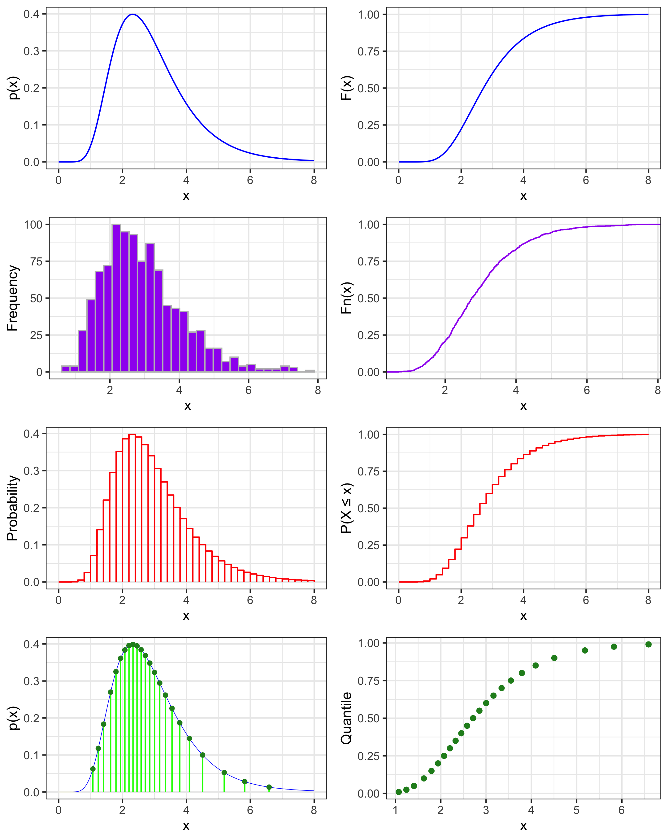
Figure 2: This figure compares the densities and CDFs of forecast representations discussed in the left and right columns respectively. Each is generated from a Lognorma(1,0.4) distribution truncated on $[0,8]$. Blue shows the density and CDF functions. Purple shows a histogram and ECDF of 1,000 samples. Red shows bin probabilities and the CDF function for a bin distribution. Green shows quantiles with corresponding values.

2.3 Mixture distributions

A mixture distribution forecast representation is an attractive alternative to the four representations already discussed. A mixture distribution forecast would allow for a large range of distribution shapes, a high resolution, storage comparable to that of bin and quantile forecasts, and ensemble construction using MA. A mixture distribution may be constructed in the same way as the ensemble described in section 2.2.1 (1) where for $C$ distributions with pdfs $p_{c}(x)$ and $w_{c}>0$ and $\sum w_{c}=1$ we have (14).

$$p^{M}(x)=\sum_{c=1}^{C}w_{c}p_{c}(x)$$ (14)

Like a parametric distribution, a mixture distribution may be evaluated using existing software like the distr package in R [32]. And scoring may be done using the LogS, CRPS, and IS. A mixture distribution, like its parametric distribution components, has an infinite resolution. A mixture distribution may be more flexible than a single component parametric distribution in terms of distribution shape. According to McLachlan and Peel, a mixture of normal densities with common variance may be used to approximate arbitrarily well any continuous distribution [33] (see also [34]). Thus, for an unconventional probability distribution –such as an MCMC posterior sample– it may be reasonable to approximate the distribution by fitting those samples to a mixture of normal distributions. Depending on the number of components a forecaster includes in a mixture forecast, the amount of storage per forecast might be as little as for a parametric forecast or as much as is permitted in the specific collaborative forecast project.

An ensemble model may be constructed by using (1) only replacing $p_{m}$ with $p_{m}^{M}$ from (14). Solving for weights may also be done by maximizing the likelihood of the forecast or minimizing the CRPS. However with the added complexity of component models being mixture distributions the computation is likely to be more expensive. An example where this is true is when minimizing the CRPS when the exact mixture distribution does not produce a closed form CRPS [2]. In large projects like the COVID-19 Forecast Hub, if an equal weight is not assigned to each component, it may be determined that models not reaching a certain standard of predictive performance are assigned an ensemble weight of 0. This would simplify an ensemble model to include only the best performing forecasts.

Table 4 shows how a mixture distribution forecast compares with the other formats discussed in terms of methods for scoring, information and resolution provided, methods for ensemble building, and computer storage requirement. To summarize, a continuous mixture distribution has the infinite resolution of a parametric distribution with the flexibility of a bin distribution, a sample distribution, and a set of quantiles. The common proper scoring rules LogS and CRPS may be used to score a mixture forecast. The storage requirement is comparable to that of a bin distribution or a set of quantiles. And MA may be used for building an ensemble. In Section 3 we show how a mixture distribution may be constructed, scored, and used to construct an ensemble using software available in R.

Table 4: This table compares scoring, information, ensemble building, and storage requirements for the different forecast representations discussed. To summarize a continuous mixture distribution has the infinite resolution of a parametric distribution with the flexibility of a bin distribution, a sample distribution, and a set of quantiles. The common proper scoring rules LogS and CRPS may be used to score a mixture forecast. The storage requirement is comparable to that of a bin distribution or a set of quantiles. And MA may be used for building an ensemble.

Type	Scoring			Ensemble			Resolution	Storage	Shape/Flexibility
	LogS	CRPS	IS	MA	QA	Sample
Bins	x	x	x	x	x	x	# bins	100s	limited by binning scheme
Quantiles			x		x		# quantiles	10s	unknown shape, no tail info
Parametric	x	x	x	x	x	x	$\infty$	10	well known distributions
Sample		x	x		x	x	$n$ draws	1000	flexible shape
Mixture	x	x	x	x	x	x	$\infty$	10s	flexible shape

3 Mixture distributions in a collaborative forecast project

The CDC flu competition and the COVID-19 Forecast Hub as well as other collaborative projects have their own established systems for receiving, scoring, and constructing ensemble forecasts. A transition from using bin or quantile forecasts to using mixture distribution forecasts would require a few adjustments to those systems. In this section we outline how some of these adjustments may be implemented. We also present tools which may be used to build forecasts from submissions, score those forecasts, and construct ensembles from them.

3.1 Submission format

For a collaborative forecast project to run smoothly, forecast submissions from all forecasters should follow the same format. For both the CDC flu competition and the COVID-19 Forecast Hub, teams provide a .csv spreadsheet which contains the distributional information for one or multiple forecasts. Tables 5 and 6 show what variables are included in those submissions and a couple rows to illustrate possible values. The column variables include location, target, type, unit, bin or quantile, and value. Here location defines the specific county, state, or country of the forecast. The target variable defines what is forecast with levels: season onset, deaths, hospitalizations, etc. The type variable defines the type for the value variable with levels of point, bin, or quantile. The unit variable defines the time frame of the forecast with levels of one week, two weeks, four weeks, etc. The variables bin and quantile give a specific bin or a specific quantile. The value variable is a number that either gives the probability associated with a bin or the value associated with a quantile.

A single submission may include many forecasts aimed at forecasting different combinations of location, target, and unit. A set of rows which share the same specific combination of location, target, and unit constitute a single forecast. One forecast for the CDC flu competition may require up to 131 rows whereas in the COVID-19 Forecast Hub one forecast may require up to 23 rows.

Table 5: This table shows a few rows of a submission file for a bin forecast like those in the CDC flu competition. A set of rows which share the same combination of location, target, and unit make up a single forecast. One submission may include many forecasts specified by differing combinations of those three columns.

location	target	type	unit	bin	value
us national	season onset	bin	week	0.0	.
us national	season onset	bin	week	0.1	.
…	…	…	…	…	…

Table 6: This shows a few rows of a submission file for a quantile forecast like those in the COVID-19 Forecast Hub. A set of rows which share the same combination of location, target, and unit make up a single forecast. One submission may include many forecasts specified by differing combinations of those three columns.

location	target	type	unit	quantile	value
us national	season onset	quantile	week	0.01	.
us national	season onset	quantile	week	0.025	.
…	…	…	…	…	…

Table 7 illustrates adjustments made to the submission formats from Tables 5 and 6 which make a usable submission format for mixture distribution forecasts. In such a format, each row represents one component distribution used in a mixture distribution. The variables bin or quantile and value are removed and replaced with family, param1, param2, and weight where family is the distribution family of the component, param1 and param2 are the parameters for the component distribution, and weight is the weight $w_{i}$ for the $i^{th}$ component.

Table 7: This is an example of a submission file for a disease outbreak forecast using a mixture distribution representation. Each row represents a component distribution of a mixture distribution. The variables location, target, and unit specify what is being forecast. The variable type specifies that the row represents a parametric distribution. The variables family, param1, and param2 specify the exact component distribution. And the variable weight specifies the weight $w_{i}$ that the $i^{th}$ component distribution is assigned in the mixture distribution. Here two components are shown with distributions Normal$(a_{n},b_{n})$, Lognormal$(a_{l},b_{l})$ and weights $w_{1}$ and $w_{2}$.

location	target	type	unit	family	param1	param2	weight
us national	season onset	dist	week	norm	$a_{n}$	$b_{n}$	$w_{1}$
us national	season onset	dist	week	lnorm	$a_{l}$	$b_{l}$	$w_{2}$
…	…	…	…	…	…	…	…

For reasons of storage and computation, a forecast project may have a limit to the number of components allowed per forecast. For reference, a mixture distribution forecast following the format in table 5 with 17 components would require $17\times 8=136$ pieces of information submitted per forecast. A submission to the COVID-19 Forecast Hub forecast with 23 quantiles according to the format in Table 5 requires $23\times 6=138$ cells. Thus if the COVID-19 Forecast Hub were to change the forecast representation from quantile forecasts to mixture forecasts but continue allowing the same amount of data per forecast, a mixture distribution with 17 components could be used in one forecast. That many components could allow for a large range of distribution shapes and flexible forecasts.

In the remainder of this section, explanations of how to work with mixture distributions submitted according to Table 7 are given. Also given is R code which demonstrates constructing a mixture distribution from a forecast submission, scoring the forecast, and building an ensemble from two separate submissions.

3.2 Mixture construction and scoring tools

A single .csv submission file of the format in Table 7 may contain multiple forecasts forecasting different combinations of location, target, and unit. Selecting only rows which share a specific combination of location, target, and unit will produce a table representing a single forecast. That table may look like Tables 8 and 9. If the table is saved as a standard data.frame in R, then tools based on the distr package [32] may be used for evaluating a mixture distribution with the component distributions in the table.

The distr package contains a function UnivarMixingDistribution() which takes as arguments a list of distributions and a vector of weights for each distribution and an object of class AbscontDistribution is returned. An AbscontDistribution class is a mother class which defines a random number generator, pdf, CDF, and quantile function for continuous distributions from common families contained in the distr package and for mixture distributions with component distributions from those families. We wrote a function MakeDist() (see APPENDIX) which takes on a data.frame with variables family, param1, param2, param3, and weight and where each row represents a component distribution in a mixture distribution. The function MakeDist() calls on the UnivarMixingDistribution() function and returns a mixture distribution object of class AbscontDistribution.

If a forecast such as in Table 8 is taken as an argument in MakeDist(), the resulting mixture distribution may then be evaluated with functions for the pdf, CDF, quantile function, and random samples from the mixture distribution may be drawn. The distribution may then be scored using the LogS or CRPS.

Table 8: This is an illustrative example of a mixture distribution forecast where the distribution is described in a data frame. The first component is a Lognormal$(2,1)$ with a weight of 0.3 in the mixture and the second component is a Normal$(2.1,1)$ with a weight of 0.7. The distribution family abbreviations are capitalized here because that is how they will be requested in the MakeDist() function. Refer to Table 13 in the APPENDIX for more details.

family	param1	param2	param3	weight
Lnorm	2	1	NA	0.3
Norm	2.1	1	NA	0.7

Table 9: This is a second illustrative example of a mixture distribution forecast where the distribution is described in a data frame. The first component is a Normal$(1.5,1)$ with a weight of 0.4 in the mixture and the second component is a Normal$(4,2)$ with a weight of 0.6. The distribution family abbreviations are capitalized here because that is how they will be requested in the MakeDist() function. Refer to Table 13 in the APPENDIX for more details.

family	param1	param2	param3	weight
Norm	1.5	1	NA	0.4
Norm	4	2	NA	0.6

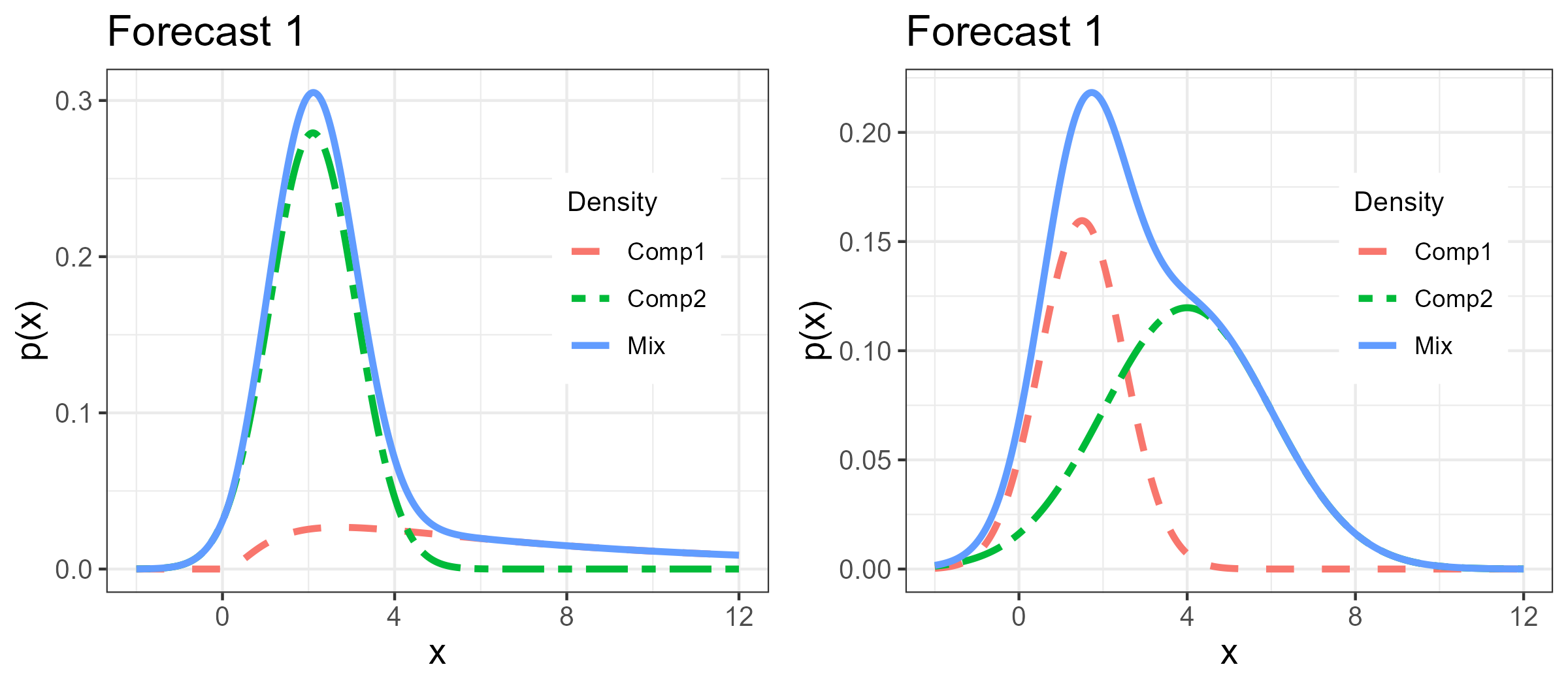
Figure 3: These plots show the density functions of the two example mixture distribution forecasts along with the component density functions scaled by the corresponding weights

Here we include code to illustrate the process of constructing and scoring two separate forecasts. We suppose that Table 8 represents a submitted forecast from one forecaster and Table 9 represents a forecast of the same event from a second forecaster. Table 3 shows plots of the pdfs for both mixture forecasts. Note the additional param3 variable in Tables 8 and 8. This variable is included in the table because of the functionality of the MakeDist() function which allows for component distributions of up to three parameters. The code here shows these two forecasts as data.frames and how the MakeDist() function is used to create the distributions in R. Once the distributions are created as AbscontDistribution objects, then functions for evaluating a pdf and a CDF for each are created.

preddf1

##   family param1 param2 param3 weights
## 1  Lnorm    2.0      1     NA     0.3
## 2   Norm    2.1      1     NA     0.7

preddf2

##   family param1 param2 param3 weights
## 1   Norm    1.5      1     NA     0.4
## 2   Norm    4.0      2     NA     0.6

#make mixture distributions from prediction submissions
mdist1 <- MakeDist(preddf1)
mdist2 <- MakeDist(preddf2)

#make pdfs for mixture predictions
dmdist1 <- function(x) {distr::d(mdist1)(x)}
dmdist2 <- function(x) {distr::d(mdist2)(x)}

#make cdfs for mixture predictions
pmdist1 <- function(x) {distr::p(mdist1)(x)}
pmdist2 <- function(x) {distr::p(mdist2)(x)}

The LogS or the CRPS may then be calculated for each forecast using the pdf and CDF functions respectively. Here will will assume that the true value which both forecasts attempted to predict was 3. The CRPS() function here is one that we wrote and is included in the APPENDIX. It is seen in the code below that under the LogS, forecast 1 from Table 8 outperforms forecast 2 from Table 9 with scores of 1.547 and 1.849 respectively. However, under the CRPS, forecast 2 outperforms forecast 1 with scores 0.635 and 0.635 respectively. We continue to use these same forecasts in Section 3.3 used in constructing an ensemble forecast.

#realized observation
xstar <- 3

#LogS for predictions at the realized observation
-log(dmdist1(xstar))

## [1] 1.547238

-log(dmdist2(xstar))

## [1] 1.848796

#CRPS for predictions at the realized observation
CRPS(pmdist1,y=xstar)

## [1] 0.6348212

CRPS(pmdist2,y=xstar)

## [1] 0.5306083

3.3 Ensemble construction

To construct an ensemble distribution from multiple mixture distributions, the UnivarMixingDistribution() function may be used. The function takes two or more AbscontDistribution distribution objects, including mixture distribution objects, and a vector of weights corresponding to each object. A new AbscontDistribution object is returned as an ensemble of mixture distributions as in (1). Since they are AbscontDistribution objects, mdist1 and mdist2 created in the code in Section 3.2 may be input as arguments into the function UnivarMixingDistribution(), but weights for each object also need to be determined.

At the onset of a collaborative forecast before there are true event observations which the forecasts may be scored on, it may make sense to assign an equal weight to each component distribution in an ensemble. As a project progresses, however, assigning weights based on past performance may be desired. As mentioned in section 2.2.1, weights may be selected by maximizing the likelihood of (1) or by minimizing the CRPS. Another method of selecting weights is to use the posterior model probability.

If we have $T$ models $M_{1},...,M_{T}$ the posterior model probability of $M_{t}$ is defined as in (15) where $p(\cdot|M_{t}):=p_{t}(\cdot)$ is the pdf of the model distribution and $p(M_{t})$ is the prior probability assigned to the model. A common approach is to assume the prior probabilities for each model are equal or $p(M_{t})=1/T$ for all $t$ in which case (15) is reduced to (16). In this case the posterior model probability for the $t^{th}$ model is equal to the exponential of its negative LogS or $p(M_{t}|x)=e^{-\text{LogS}(p(M_{t}|x))}$, so the performance of a forecast based on the LogS is directly related to its posterior model probability and may be used as an ensemble weight. For an observed event $x^{*}$, ensemble weights $(w_{t})$ from (1) may be defined as $w_{t}:=p(M_{t}|x^{*})$.

$$p(M_{t}|x)=\frac{p(x|M_{t})p(M_{t})}{p(x)}=\frac{p(x|M_{t})p(M_{t})}{\sum_{k=1}^{T}p(x|M_{k})p(M_{k})}$$ (15)

$$p(M_{t}|x)=\frac{p(x|M_{t})}{\sum_{k=1}^{T}p(x|M_{k})}$$ (16)

Using the illustrative example from Section 3.2, the following code shows how to use the posterior model probability to select weights, construct an ensemble distribution, and score the ensemble forecast. Here again we take the true event value to be 3. The ensemble distribution along with component distributions is shown in Figure 4.

#posterior model probability for calculating weights
w1 <- pmdist1(xstar)/(pmdist1(xstar) + pmdist2(xstar))
w2 <- 1-w1
w1

## [1] 0.5286434

w2

## [1] 0.4713566

#build ensemble with calculated weights
ensdist <- distr::UnivarMixingDistribution(mdist1,
                                           mdist2,
                                           mixCoeff = c(w1,w2))

#pdf and cdf for ensemble
densdist <- function(x) {(distr::d(ensdist)(x))}
pensdist <- function(x) {(distr::p(ensdist)(x))}

#LogS for predictions at the realized observation
-log(densdist(xstar))

## [1] 1.678156

#CRPS for predictions at the realized observation
CRPS(pensdist,y=xstar)

## [1] 0.5486368

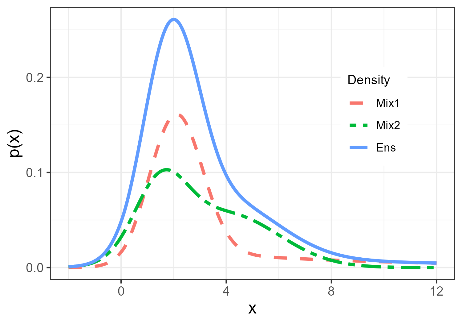
Figure 4: Ensemble forecast made from forecast 1 and forecast 2 from Section 3.2. The red line is the density component of mixture forecast 1 with weight 0.529. The green line is the density component of mixture forecast 2 with weight 0.471. The blue line is the density of the ensemble forecast.

4 Retrospective analysis

For large collaborative forecast projects having already established the representation formats for forecasting, it may be difficult for teams to adjust to using mixture distributions. There may be several reasons for this, including that not all forecast modeling methods will produce forecasts which may conveniently be represented by a mixture distribution. In this section we attempt to assess whether or not bin forecasts from the CDC flu competition or quantile forecasts from the COVID-19 Forecast Hub may be reasonably approximated by a mixture distribution with normal components as the number of components in the distribution increases.

Forecasters in both the CDC flu competition and the COVID-19 Forecast Hub do not include with their forecast submissions information about modeling methods or distributional assumptions. Thus the only information we have for fitting distributions are bin forecasts and quantile forecasts. We are unaware of formal statistical methods for fitting parametric distributions or mixture distributions to bin distributions. Methods of fitting a distribution to quantiles include Bayesian Quantile Matching [35], step interpolation with exponential tails [36], and the Method of Simulated Quantiles [37]. These studies, however, lack claims that the methods for fitting are statistically formal. Nirwan and Bertshinger state that minimizing the mean square error between quantile values and a CDF function has been the most common way to fit a distribution to a set of quantiles. This is the method we will use in Section 4.2. Because of the lack of statistically formal methods for fitting a parametric distribution to a bin distribution or a set of quantiles, it should be noted that any conclusions made in this section may not be stated in terms of statistical certainty.

4.1 CDC flu competition

The CDC Retrospective Forecasts project on zoltrdata.com [38] contains 869,638 probabilistic influenza-like illness forecasts for all combinations of 11 regions in the United States and seven targets from 27 different modeling teams. These include forecasts made during all flu seasons between October 2010 and December 2018. All forecasts are represented by bin distributions.

To assess whether the bin probabilities may be more closely approximated by mixture distributions with an increasing number of components, 5 mixture distributions with one to five normal components were fit to each of a selected set of bin forecasts. In fitting a distribution to a forecast, we want minimize (17). Equation (17) is a variation of the Kullback Leibler divergence (KLD). Here $\bm{p}$ represents a bin distribution where $p_{i}>0$ is the reported probability for the $i^{th}$ bin $B_{i}:=[b_{i-1},b_{i})$, and $K$ is the number of bins. $M_{\theta}^{C}$ is a random variable of a mixture distribution with $C$ components and parameter vector $\theta$. The fitted parameter vector $\hat{\theta}$ is the solution to (18).

$$D(\bm{p}|M_{\theta})=\sum_{i=1}^{K}p_{i}\text{log}\left(\frac{p_{i}}{P(M^{C}_{\theta}\in B_{i})}\right)$$ (17)

$$\hat{\theta}=\underset{\theta}{\operatorname{argmin}}\sum_{i=1}^{K}p_{i}\text{log}\left(\frac{p_{i}}{P(M^{C}_{\theta}\in B_{i})}\right)$$ (18)

Pulling forecasts from zoltardata.com and fitting mixture distributions to them was computationally expensive, so we limited the analysis to 1,141 forecasts. To select these forecasts, we sampled from the 869,638 forecasts as follows. For each submission -a single submission may contain multiple forecasts for various units and targets forecasted- there is a recorded date corresponding to the week of the forecast. There are 246 total dates. The number of submissions for each week was counted and 10 weeks were randomly selected with probabilities based on the number of submissions by week. All submissions from the selected 10 weeks were pulled from zoltardata.com, but the only forecasts kept for fitting were US national level forecasts for 1, 2, 3, and 4 week ahead and season peak percentage and forecasts with more 4 bins. Twenty-six of twenty-seven teams were represented by the selected forecasts.

With forecasts selected, we then fit five mixture distributions to each. For each distribution to be fit there are $C\in\{1,2,3,4,5\}$ normal components. In the mixture distribution there are $C$ mean values, a common standard deviation shared by each component, and $C$ component weights $\omega_{1},...,\omega_{C}$. Thus the parameter vector $\theta=(\mu_{1},...,\mu_{C},\sigma,\omega_{1},...,\omega_{C})$.

To ensure in the optimization that $\omega_{1},...,\omega_{C}>0$ and $\sum_{i=1}^{C}\omega_{i}=1$ we optimize the parameters $\nu_{1}=0,...,\nu_{C}$ and set $\omega_{i}=\frac{e^{\nu_{i}}}{\sum_{i=1}^{c}e^{\nu_{i}}}$. Since $\nu_{1}=0$, only the $C-1$ parameters $\nu_{2},...,\nu_{C}$ parameters are optimized. To maintain order in the set of mixture components, we add the constraint $\mu_{1}<\mu_{2}<...<\mu_{C}$. This is enforced by taking $\mu_{1}=\mu_{1},\mu_{2}=\mu_{1}+e^{\alpha_{1}},...,\mu_{C}=\mu_{C-1}+e^{\alpha_{C-1}}$ so that the optimized parameters for means are $\mu_{1},\alpha_{1},...,\alpha_{C-1}$. The necessary condition that $\sigma>0$ is enforced by setting $\sigma=e^{\eta}$ and optimizing over $\eta$. Thus the $2C$ parameter vector to be optimized is $\gamma=(\mu_{1},\alpha_{1},...,\alpha_{C-1},\eta,\nu_{2},...\nu_{C})$. The optimization was done iteratively by repeating the following steps.

1. Initialize $\gamma_{0}=(\mu_{1}^{(0)},\alpha_{1}^{(0)}...,\alpha_{C-1}^{(0)},\eta^{(0)},\nu_{2}^{(0)},...,\nu_{C}^{(0)})$

2. At step $m\geq 1$, set the following $2C$ parameter vectors where

$$\gamma_{1}^{(m)}=(\tilde{\mu_{1}}^{(m+1)},\alpha_{1}^{(m)}...,\alpha_{C-1}^{(m)},\eta^{(m)},\nu_{1}^{(m)},...,\nu_{C}^{(m)})$$

$$\gamma_{2}^{(m)}=(\mu_{1}^{(m)},\tilde{\alpha_{1}}^{(m+1)}...,\alpha_{C-1}^{(m)},\eta^{(m)},\nu_{1}^{(m)},...,\nu_{C}^{(m)})$$

$$\vdots$$

$$\gamma_{2C}^{(m)}=(\mu_{1}^{(m)},\alpha_{1}^{(m)}...,\alpha_{C-1}^{(m)},\eta^{(m)},\nu_{1}^{(m)},...,\tilde{\nu_{C}}^{(m+1)})$$

where $\gamma_{i}^{(m)}$ is the parameter vector minimizing (18) over the $i^{th}$ element while holding all other elements constant.

3. Set $\gamma^{(m+1)}=\underset{\gamma_{i}^{(m)}}{\operatorname{argmin}}\sum_{i=1}^{K}p_{i}\text{log}\left(\frac{p_{i}}{P(M_{\gamma_{i}^{(m)}}\in B_{i})}\right),i\in(1,...,2C)$

4. Return to step 2.

This process was run until $|D(p||M_{\theta^{(m+1)}}-D(p||M_{\gamma^{(m)}})|/D(p||M_{\gamma^{(m)}})<0.001$ where $D(p||M_{\theta})$ is as defined in (17), or $m=500$. The optimization was done using the optim function in R, and the optimization algorithm used was either ”BFGS” or ”L-BFGS-B”. Of the 1,141 selected forecasts, 1,103 were fit by the 5 mixture distributions. The remaining forecasts were ignored in further analysis because the fitting algorithms failed to converge.

Figure 5 shows boxplots of KLD for all fit mixture distributions for 1 to 5 components. In general, the KLD between the actual forecast distribution and the fit distribution tends to decrease as the number components in the fit mixture distribution increases. Figure 6 shows examples of density functions of one to five components fit to a forecast. The outer plots show fit mixture density functions plotted over the bin probabilities where the probabilities are multiplied by 10 to give the same scale as the densities. The inner plots show the KLD of the forecast and the fit distribution by number of components in the mixture distribution.

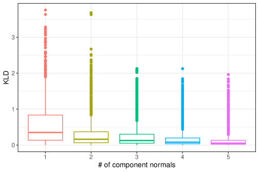
Figure 5: Each boxplot is made of the KLD from equation (17) calculated for each sampled flu forecast. As the number of component normals fit to the forecasts increases, the median values and spread decrease.

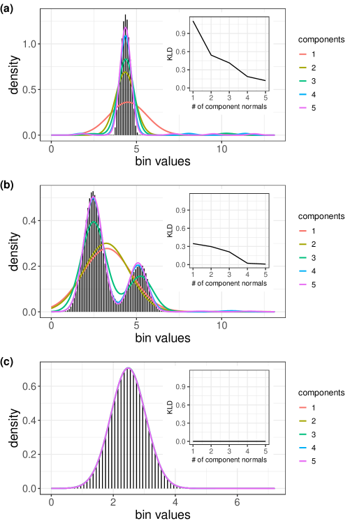
Figure 6: Three selected flu forecasts with the pdfs of mixture distributions of one to five components plotted on top. The inner plot shows the KLD value as the number of components increases. The bin probabilities are multiplied by 10 to ensure they are on the same scale as the pdfs in the plot.

To further compare the fits to the forecasts, we compared the actual forecast performance of the bin forecast to the fit mixture distributions. For each week and target represented in the sample of selected forecasts, truth data was obtained. For each bin forecast, the bin in which the true value fell, $B_{t}$ was determined and the probability value in that bin was noted as $p_{t}$. Then for each mixture distribution fit to that density, the probability $p^{M^{C}}_{t}=P(M^{C}\in B_{t})$ within the true bin was calculated. All forecasts were then classed by the specific target and week for which they were forecasting. There were 50 total combinations of target and week. Figure 7 shows 5 scatterplots where the probabilities $p_{t}$ for for 1 week ahead forecasts on 2016-10-17 are plotted against the probabilites $p^{M^{C}}_{t}$. Each plot represents a different number of component distrubtions in the mixture distribution fit. The linear correlation coefficient between the probabilites is also given, and the correlation increases as the number of components increases. Table 10 shows the same correlation trend for 5 different target/week combinations and for all forecasts not broken out by target/week combinations.

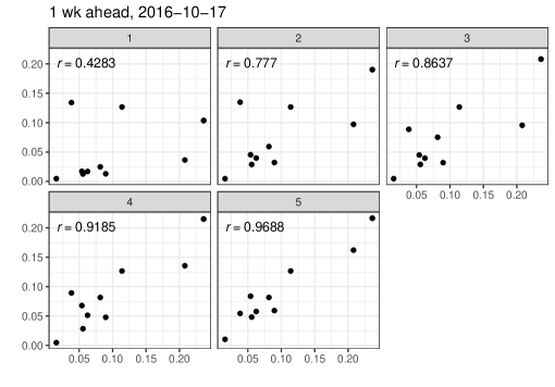
Figure 7: Scatterplots with $p_{t}$ on the x-axis and $p_{t}^{M^{C}}$ on the y-axis for all selected 1 week ahead forecasts for the date 10/17/16. The correlation between the probabilities increases as the number of components in the fit mixture increases suggesting that the forecasts may be more closely approximated as the number of components increases.

Table 10: (a) 10/28/13 Season peak, (b) 12/2/13 4 wk, (c) 10/17/16 season peak, (d) 4/20/15 4 wk, (e) 4/20/15 1 wk. The values are the correlations between the actual probability score from the submitted forecasts and the probability according to the fit mixture distributions.

Components	Overall	(a)	(b)	(c)	(d)	(e)
1	0.5811	0.7608	0.789	0.4454	0.748	0.4752
2	0.738	0.9428	0.8885	0.6349	0.8025	0.8264
3	0.8341	0.9567	0.9626	0.7610	0.8271	0.8503
4	0.8445	0.978	0.9715	0.9428	0.7874	0.9114
5	0.8920	0.9844	0.9903	0.9691	0.7188	0.9454

4.2 COVID-19 Forecast Hub

As of October 2022 there were over 100 million forecasts from 122 different modeling teams submitted to the COVID-19 Forecast Hub [39]. These forecasts covered all combinations of 3,202 municipalities (mostly counties) in the United States with 441 target/unit combinations. The first of these forecasts was submitted in March of 2020 shortly after the initial outbreak of the COVID-19 virus in the US, and forecasts have been received weekly since then. The forecasts are all quantile forecasts made up of three or 11 predictive intervals –depending on the specific unit for the forecast– and a median. Thus each forecast includes seven or 23 quantiles.

As in the retrospective study of influenza forecasts, we wanted to assess whether or not we can more closely approximate the quantile forecasts by increasing the number of components in a mixture distribution. Fitting a mixture distribution to a set of quantiles was done in the same manner as to bin probabilities, only by choosing the parameter $\hat{\theta}$ which minimizes the sum of square differences (SS) between the quantiles and the CDF of a mixture distribution as in equation (19). Here $\hat{\theta}$ is the solution to equation (20). In equation (19), $q_{i}$ is the $i^{th}$ quantile (out of $N$ quantiles) from a forecast and $F(\alpha_{i}|\hat{\theta})$ is a fit CDF evaluated at the value $\alpha_{i}$ with parameter $\hat{\theta}$. The parameter $\hat{\theta}$ is the solution to (20).

$$\text{SS}=\sum_{i=1}^{m}(q_{i}-F(\alpha_{i}|\hat{\theta}))^{2}$$ (19)

$$\hat{\theta}=\arg\min_{\theta}\sum_{i=1}^{m}(\alpha_{i}-F(q_{i}|\theta))^{2}$$ (20)

We randomly selected 9 weeks from which to pull forecasts from zoltardata.com by searching through all teams which submitted any forecast. Forecasts submitted between a Monday and the following Tuesday were considered to have come from the same week [40]. The 9 weeks were selected randomly with probability relative to the total number of forecasts submitted that week. From those weeks, only US national forecasts for increasing and cumulative deaths from one to four weeks ahead were selected for fitting. In total, 2,676 forecasts were selected. However, as in the influenza analysis, computational issues made it difficult to fit five different mixture distributions to all quantile forecasts, as well truth data was missing for two targets during one week in September 2022. Thus the remainder of the anlysis included 2,319 forecasts.

Table 11 shows the maximum SS values over all fits for fits from one to five component mixture distributions. Figure 9 contains plots showing fits for selected individual forecasts with fit CDF functions plotted over quantiles in the left plots, and SSE values plotted by the number of components.

Table 11: Maximum SS value over all quantile forecasts to which mixture distributions were fit for one to five components

Components	1	2	3	4	5
max SS	0.53	0.36	0.16	0.11	0.06

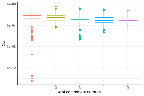
Figure 8: Boxplots of SS (on the log scale) between submitted quantile forecasts and fit CDFs

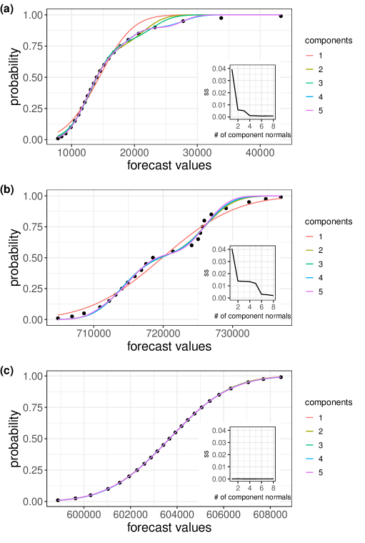
Figure 9: Actual quantiles for three different COVID-19 forecasts with CDFs of fit mixture distributions from one to five components. The inner plots show the SS value as the number of components is increased.

To compare forecast performance between actual quantile forecasts and the fit distributions, truth for each week/target combination was obtained and the WIS from (12) was calculated. Figure 10 shows plots of the WIS scores for 3 week ahead cumulative death forecasts for December 29, 2020 plotted against WIS scores for mixture distributions fit to the forecasts. There is a separate scatterplot for fits of one to five components. Table 12 shows calculated correlations between actual WIS scores and fit WIS scores for 5 different week/target combinations.

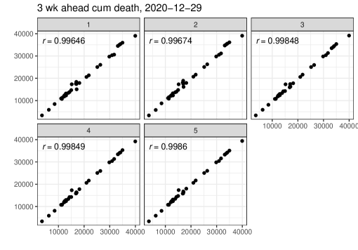
Figure 10: Scatter plots for actual WISs and WISs from fit mixture distributions for 3 week ahead COVID-19 forecasts from 12/29/2020

Table 12: Correlation between actual WIS and WIS from fit mixture distributions for selected forecasts of the following dates and targets (a) 9/20/22 2 wk cum, (b) 9/14/21 1 wk inc, (c) 12/22/20 4 wk cum, (d) 7/14/20 4 wk cum, (e) 12/22/20 2 wk cum

Components	Overall	(a)	(b)	(c)	(d)	(e)
1	0.99966	0.99999	0.99890	0.99851	0.99727	0.9968
2	0.99949	1	0.99913	0.99899	0.99762	0.99673
3	0.99959	1	0.99947	0.99961	0.99603	0.99819
4	0.9996	1	0.99945	0.99959	0.99808	0.99535
5	0.99978	1	0.99952	0.99962	0.99865	0.99788

The results from these studies suggest that forecasts in bin distribution and quantile formats may indeed be increasingly well approximated by a mixture of normal distributions as the number of components increases.

4.3 Sample Distribution Forecast

As some forecasting projects may accept sample distributions for forecasts, we created this example to show that a sample may be closely approximated by a mixture distribution as the number of components increases. To show this, we first created a sample distribution. With the sample in hand we fit a normal distribution by calclating the maximum likelihood estimates for mean and standard deviation. We then fit mixture distributions from two to five components to the sample, thus giving fits for mixture distributions of one to five component normal mixture distributions.

We obtained a sample distribution by first selecting a bin forecast from the flu forecasting competition. We randomly drew 700 samples where each draw corresponded to a bin $B_{i}$ with probability according to the forecast $p_{i}$. For each draw corresponding to each bin $B_{i}$, a value was randomly selected according to the uniform distribition $Unif(b_{i-1},b_{i})$.

The expected maximization (EM) algorithm was used to find maximum likelihood values to fit a mixture distribution to the sample. We used the function normalmixEM in the mixtools package in R for this. For each of the five fits, we calculated the Kolmogorov-Smirnov (KS) test statistic or the maximum distance between the ECDF function of the sample and the CDF function of the fit mixture distrubtion. Figures 11 and 12 show the fit CDFs plotted with the ECDF and the pdfs plotted on the histogram respectively. These figures show that the sample is more closely approximated as the number of components in a mixture distribution increases.

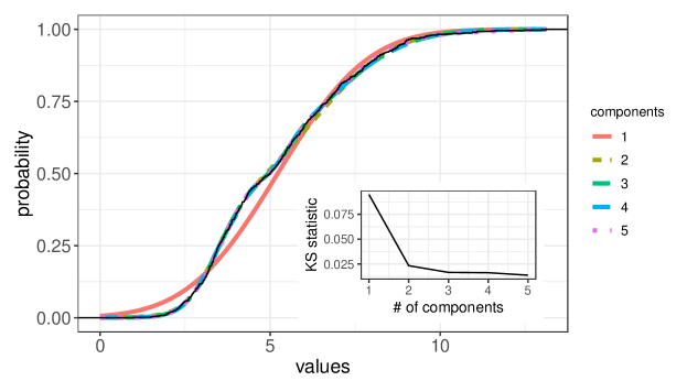
Figure 11: The outer plot shows the fit CDFs in color plotted with the ECDF in black of the sample. The inner plot shows the value of the KS statistic of the fit CDFs and the ECDF as the number of components increases.

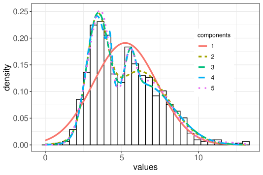
Figure 12: Histogram of the sample with pdfs of the fit mixture distributions

5 Discussion

In this paper we have reviewed four representations commonly used in probabilistic forecasting and discussed proper scoring, data storage, and ensemble model construction for each type. We presented the mixture distribution representation and argue that its use in collaborative probabilistic forecasting is preferable to the other representations. In terms of model flexibility, storage, and ensemble construction it is comparable to bin and quantile forecasts but also provides a forecast with a infinite nominal resolution. Based on a retrospective analysis, we argue that forecasts of quantile or bin distribution representations may be more closely approximated by a mixture distribution as the number of components of the distribution is increased. This may allow the transition from past and current formats to a mixture distribution format straightforward. We thus advocate for the use of mixture distributions in future forecasting projects like those done in the CDC flu competition or in the COVID-19 Forecast Hub.

For a number of reasons, some forecasters may prefer not to the adopt mixture distributions as a format in collaborative forecasting. A collaborative forecast center, along with forecasters, using a different representation format may simply not want to break from tradition. There may be some concern that a mixture distribution does not represent well certain models. And the implementation of new scoring and ensemble construction methods may also be a barrier. Development of tools beyond what was used in Section 3.2 would assist in making a transition to using mixture distributions more straightforward. One aspect of ensemble construction which received little attention in this paper is the selection of weights for components of an ensemble where each of the components is a mixture distribution. Computing requirements could be a concern in such a problem, and further research on this may provide ideas of best methods for weight selection.

Another area of recommended research is the use of joint mixture distributions for forecasting. We have only considered here probabilistic forecasting of one event at a time, or example, the number of new infections in one week at one specific location. This forecast is presented as a marginal distribution for that specific target, time, and location. A joint distribution for forecasting multiple targets, times, or locations may sometimes be desirable and may require further consideration on how joint mixture distributions could be used as a format in collaboration.

6 APPENDIX

The following is the code to make the MakeDist() function introduced in 3.2. Tables 13 and 14 show how distribution family arguments are to be written and what parameters are to be used for the distributions in the MakeDist() function.

MakeDist <- function(distsdf){

  distdf <- distsdf[distsdf[,1] != ’Lst’,]
  tdist <- distsdf[distsdf[,1] == ’Lst’,]

  fun_dist <-
    apply(distdf, FUN=function(x) {
      paste(’distr::’,x[1], ’(’,
            ifelse(!is.na(x[2]) & (!is.na(x[3]) | !is.na(x[4])),
                   paste(x[2],’,’,sep=’’),
                   ifelse(!is.na(x[2]) & is.na(x[3]) & is.na(x[4]),
                          x[2], ’’)),
            ifelse(!is.na(x[3]) & !is.na(x[4]),
                   paste(x[3],’,’,sep=’’),
                   ifelse(!is.na(x[3]) & is.na(x[4]), x[3],’’)),
            ifelse(!is.na(x[4]),x[4],’’), ’)’,sep=’’)
    }, MARGIN = 1
    )

  fun_tdist <- apply(tdist, FUN=function(x) {
    paste0(’distr::Td(’,x[4],’)*’,x[3], ’+’, x[2])
  }, MARGIN = 1
  )

  dist_args <- paste(fun_dist, collapse=’,’,sep=’’)
  tdist_args <- paste0(fun_tdist,collapse=’,’)
  args <- ifelse(tdist_args!=’’,paste(dist_args,tdist_args,sep=’,’),dist_args)

  weights <- c(distdf[,5],tdist[,5])
  mixString <- paste(’distr::UnivarMixingDistribution(’,
                     args,’,mixCoeff=weights)’,sep=’’)
  mixDist <- eval(parse(text=mixString))

  return(mixDist)
}

Table 13: This table describes how each argument may be entered into a data frame entered into the MakeDist() function, including exactly how the distribution families should appear and what paramaters should be included for each distribution family.

Argument	Summary	Options
dist	A string specifying a distribution family.	Beta, Cauchy, Lnorm, Logis, “Unif, Lst (location scale t distribution), Weibull, Fd, Norm, Chisq, Gammad, Exp Binom, Dirac, Pois, Hyper, Nbinom, Geom
param1	A real number specifying the first parameter value of the distribution.	Beta: shape1; Cauchy: location; Lnorm: meanlog; Logis: location; Unif: min; Lst: location; Weibull: shape; Fd: df1; Norm: mean; Chisq: df; Gammad: scale; Exp: rate; Binom: size; Dirac: location; Pois: lambda; Hyper: m; Nbinom: n; Geom: prob
param2	A real number specifying the second parameter value of the distribution.	Beta: shape2; Cauchy: scale; Lnorm: slog; Logis: scale; Unif: Max; Lst: scale; Weibull: scale; Fd: df2; Norm: sd; Chisq: ncp; Gammad: shape; Binom: prob; Hyper: n; Nbinom: p
param3	A real number specifying the third parameter value of the distribution.	Lst: df; Hyper: k
weight	A real number between 0 and 1 specifying the weight given to the distribution in the overall mixture distribution. The sum of the weight column should equal 1.	…

Table 14: This table shows what parameters may be used for each distribution family used in a data frame for the MakeDist() function or in the UnivarMixingDistribution() function.

Distribution	dist	param1	param2	param3
Beta	Beta	shape1	shape2
Cauch	Cauchy	location	scale
Log-normal	Lnorm	meanlog	slog
Logistic	Logis	location	scale
Uniform	Unif	min	max
Location Scale T	Lst	location	scale	df
Weibull	Weibull	shape	scale
F	Fd	df1	df2
Normal	Norm	mean	sd
Chisqure	Chisq	df
Gamma	Gammad	scale	shape
Exponential	Exp	rate
Binomial	Binom	size	prob
Dirac	Dirac	location
Poisson	Pois	lambda
Hypergeometric	Hyper	m	n	k
Negative binomial	Nbinom	n	p
Geometric	Geom	prob

The following is the code used to make the function CRPS() used in section 3.2.

crps_integrand <- function(x,dist,y) {(dist(x) - as.numeric(y <= x))^2}

CRPS <- function(y,dist) {
  int <- integrate(crps_integrand,-Inf,Inf,y,dist=dist)
  return(int$value)
}

References

- [1] Tilmann Gneiting and Matthias Katzfuss. Probabilistic forecasting. Annual Review of Statistics and Its Application, 1:125–151, 2014.
- [2] Sándor Baran and Sebastian Lerch. Combining predictive distributions for the statistical post-processing of ensemble forecasts. International Journal of Forecasting, 34(3):477–496, 2018.
- [3] Jan JJ Groen, Richard Paap, and Francesco Ravazzolo. Real-time inflation forecasting in a changing world. Journal of Business & Economic Statistics, 31(1):29–44, 2013.
- [4] Teresa K Yamana, Sasikiran Kandula, and Jeffrey Shaman. Superensemble forecasts of dengue outbreaks. Journal of The Royal Society Interface, 13(123):20160410, 2016.
- [5] Tilmann Gneiting, Fadoua Balabdaoui, and Adrian E Raftery. Probabilistic forecasts, calibration and sharpness. Journal of the Royal Statistical Society: Series B (Statistical Methodology), 69(2):243–268, 2007.
- [6] Tilmann Gneiting and Roopesh Ranjan. Combining predictive distributions. Electronic Journal of Statistics, 7:1747–1782, 2013.
- [7] Fabian Krueger, Sebastian Lerch, Thordis L Thorarinsdottir, and Tilmann Gneiting. Probabilistic forecasting and comparative model assessment based on markov chain monte carlo output. arXiv preprint arXiv:1608.06802, 12, 2016.
- [8] Craig J McGowan, Matthew Biggerstaff, Michael Johansson, Karyn M Apfeldorf, Michal Ben-Nun, Logan Brooks, Matteo Convertino, Madhav Erraguntla, David C Farrow, John Freeze, et al. Collaborative efforts to forecast seasonal influenza in the united states, 2015–2016. Scientific Reports, 9(1):1–13, 2019.
- [9] James W Taylor. Evaluating quantile-bounded and expectile-bounded interval forecasts. International Journal of Forecasting, 37(2):800–811, 2021.
- [10] Johannes Bracher, Evan L Ray, Tilmann Gneiting, and Nicholas G Reich. Evaluating epidemic forecasts in an interval format. PLoS Computational Biology, 17(2):e1008618, 2021.
- [11] CDC. Flusight: Flu forecasting. https://www.cdc.gov/flu/weekly/flusight/index.html. Accessed: 2022-02-03.
- [12] Estee Y Cramer, Yuxin Huang, Yijin Wang, Evan L Ray, Matthew Cornell, Johannes Bracher, Andrea Brennen, Alvaro J Castro Rivadeneira, Aaron Gerding, Katie House, Dasuni Jayawardena, Abdul H Kanji, Ayush Khandelwal, Khoa Le, Jarad Niemi, Ariane Stark, Apurv Shah, Nutcha Wattanachit, Martha W Zorn, Nicholas G Reich, and US COVID-19 Forecast Hub Consortium. The united states covid-19 forecast hub dataset. medRxiv, 2021.
- [13] Thomas McAndrew and Nicholas G Reich. Adaptively stacking ensembles for influenza forecasting with incomplete data. arXiv preprint arXiv:1908.01675, 2019.
- [14] Nicholas G Reich, Craig J McGowan, Teresa K Yamana, Abhinav Tushar, Evan L Ray, Dave Osthus, Sasikiran Kandula, Logan C Brooks, Willow Crawford-Crudell, Graham Casey Gibson, et al. Accuracy of real-time multi-model ensemble forecasts for seasonal influenza in the us. PLoS Computational Biology, 15(11):e1007486, 2019.
- [15] Estee Y Cramer, Velma K Lopez, Jarad Niemi, Glover E George, Jeffrey C Cegan, Ian D Dettwiller, William P England, Matthew W Farthing, Robert H Hunter, Brandon Lafferty, et al. Evaluation of individual and ensemble probabilistic forecasts of covid-19 mortality in the us. medRxiv, 2021.
- [16] Evan L Ray, Nutcha Wattanachit, Jarad Niemi, Abdul Hannan Kanji, Katie House, Estee Y Cramer, Johannes Bracher, Andrew Zheng, Teresa K Yamana, Xinyue Xiong, et al. Ensemble forecasts of coronavirus disease 2019 (covid-19) in the us. MedRXiv, 2020.
- [17] Tilmann Gneiting and Adrian E Raftery. Strictly proper scoring rules, prediction, and estimation. Journal of the American Statistical Association, 102(477):359–378, 2007.
- [18] GitHub. Github: Covid-19 forecasts. https://api.github.com/repos/reichlab/covid19-forecast-hub. Accessed: 2022-04-04.
- [19] David H Wolpert. Stacked generalization. Neural networks, 5(2):241–259, 1992.
- [20] Evan L Ray and Nicholas G Reich. Prediction of infectious disease epidemics via weighted density ensembles. PLoS computational biology, 14(2):e1005910, 2018.
- [21] Adrian E Raftery, Tilmann Gneiting, Fadoua Balabdaoui, and Michael Polakowski. Using bayesian model averaging to calibrate forecast ensembles. Monthly Weather Review, 133(5):1155–1174, 2005.
- [22] Jasper A Vrugt, Cees GH Diks, and Martyn P Clark. Ensemble bayesian model averaging using markov chain monte carlo sampling. Environmental Fluid Mechanics, 8(5):579–595, 2008.
- [23] Eric-Jan Wagenmakers and Simon Farrell. Aic model selection using akaike weights. Psychonomic bulletin & review, 11:192–196, 2004.
- [24] Hans Hersbach. Decomposition of the continuous ranked probability score for ensemble prediction systems. Weather and Forecasting, 15(5):559–570, 2000.
- [25] Jose-Henrique GM Alves, Paul Wittmann, Michael Sestak, Jessica Schauer, Scott Stripling, Natacha B Bernier, Jamie McLean, Yung Chao, Arun Chawla, Hendrik Tolman, et al. The ncep–fnmoc combined wave ensemble product: Expanding benefits of interagency probabilistic forecasts to the oceanic environment. Bulletin of the American Meteorological Society, 94(12):1893–1905, 2013.
- [26] Subrata Chakraborty. Generating discrete analogues of continuous probability distributions -a survey of methods and constructions. Journal of Statistical Distributions and Applications, 2(1):1–30, 2015.
- [27] Logan C Brooks, Evan L Ray, Jacob Bien, Johannes Bracher, Aaron Rumack, Ryan J Tibshirani, and Nicholas G Reich. Comparing ensemble approaches for short-term probabilistic covid-19 forecasts in the us. International Institute of Forecasters, 2020.
- [28] Nicholas G Reich, Logan C Brooks, Spencer J Fox, Sasikiran Kandula, Craig J McGowan, Evan Moore, Dave Osthus, Evan L Ray, Abhinav Tushar, Teresa K Yamana, et al. A collaborative multiyear, multimodel assessment of seasonal influenza forecasting in the united states. Proceedings of the National Academy of Sciences, 116(8):3146–3154, 2019.
- [29] Adrienne W Kemp. Classes of discrete lifetime distributions. Communications in Statistics – Theory and Methods, 33(12):3069–3093, 2004.
- [30] GitHub. Github: Cdc flusight hospitalization forecasts. https://github.com/cdcepi/Flusight-forecast-data/blob/master/README.md. Accessed: 2023-09-23.
- [31] Konrad Bogner, Katharina Liechti, and Massimiliano Zappa. Combining quantile forecasts and predictive distributions of streamflows. Hydrology and Earth System Sciences, 21(11):5493–5502, 2017.
- [32] Florian Camphausen, Matthias Kohl, Peter Ruckdeschel, Thomas Stabla, and Maintainer Peter Ruckdeschel. The distr package. 2007.
- [33] DAVID Peel and G MacLahlan. Finite mixture models. John & Sons, 2000.
- [34] Hien D Nguyen and Geoffrey McLachlan. On approximations via convolution-defined mixture models. Communications in Statistics-Theory and Methods, 48(16):3945–3955, 2019.
- [35] Rajbir-Singh Nirwan and Nils Bertschinger. Bayesian quantile matching estimation. arXiv preprint arXiv:2008.06423, 2020.
- [36] Joaquin Quinonero-Candela, Carl Edward Rasmussen, Fabian Sinz, Olivier Bousquet, and Bernhard Schölkopf. Evaluating predictive uncertainty challenge. In Machine Learning Challenges Workshop, pages 1–27. Springer, 2005.
- [37] Yves Dominicy and David Veredas. The method of simulated quantiles. Journal of Econometrics, 172(2):235–247, 2013.
- [38] Zoltar. Zoltardata: Cdc retrospective forecasts. https://zoltardata.com/project/6. Accessed: 2022-04-04.
- [39] Zoltar. Zoltardata: Covid-19 forecasts. https://zoltardata.com/project/44. Accessed: 2022-04-04.
- [40] GitHub. Github: Cdc flusight ensemble. https://github.com/FluSightNetwork/cdc-flusight-ensemble/blob/master/README.md. Accessed: 2023-09-23.