Tradeoff relations for simultaneous measurement of multiple incompatible observables and multi-parameter quantum estimation

Abstract

How well can multiple noncommutative observables be implemented by a single measurement? This is a fundamental problem in quantum mechanics and determines the optimal performances of many tasks in quantum information science. While existing studies have been mostly focusing on the approximation of two observables with a single measurement, in practice multiple observables are often encountered, for which the errors of the approximations are little understood. Here we provide an approach to study the approximation of an arbitrary finite number of observables with a single measurement. With this approach, we obtain analytical bounds on the errors of the approximations for an arbitrary number of observables, which significantly improves our understanding of a fundamental problem. We also provide a tighter bound in terms of the semi-definite programming, which, in the case of two observables, can lead to an analytical bound that is tighter than existing bounds. We then demonstrate the power of the approach by quantifying the tradeoff of the precisions for the estimation of multiple parameters in quantum metrology, which is of both fundamental and practical interest.

I Introduction

A central feature of quantum mechanics is the noncommutativity, which plays a fundamental role in quantum physics. The most widely studied scenario of the non-commutativity is the non-commutativity of the observables, which lies at the heart of quantum mechanics and has propelled many discoveries of new phenomena deviating from classical physics. It is well known that when multiple observables commute with each other then they can be simultaneously measured by a projective measurement on the common eigenspaces. When they do not commute, however, they can only be approximately implemented. A key question is then how well a single measurement can measure multiple noncommuting observables. Intuitively the noncommuting observables can only be approximately measured simultaneously and there will exist a tradeoff between the errors of the approximation. The better one observable is measured, the larger the errors on the approximation of other incompatible observables. Such tradeoff is closely related to the uncertainty principle [1], one of the pillars of quantum mechanics.

The standard Robertson-Schrödinger uncertainty relation [2, 3], $(\Delta X_{1})^{2}(\Delta X_{2})^{2}\geq\frac{1}{4}|\mathrm{Tr}(\rho[X_{1},X_{2}])|^{2}$ with $(\Delta X_{1/2})^{2}=\langle X_{1/2}^{2}\rangle-\langle X_{1/2}\rangle^{2}$, describes the impossibility of preparing quantum states with sharp distributions for multiple non-commuting observables simultaneously. This is also called the preparation uncertainty relation. The uncertainty relations that describe the approximation of multiple non-commuting observables via a single measurement are called measurement uncertainty relations [5, 6, 7, 8, 9, 10, 11, 12, 13, 14, 15, 16, 17, 18, 19]. There are two main approaches to measurement uncertainty relations: state-independent relations that study the uncertainty of the measurement device over all input states [19, 18, 20, 21, 22, 23], and state-dependent relations that characterize the error-tradeoff for joint measurements on a given input state [5, 6, 7, 8, 9, 10, 11, 12, 13, 14, 16, 15]. In this article, we focus on the state-dependent measurement uncertainty relations, as we are interested in applications to quantum estimation where the state is often restricted.

In the case of two observables, Ozawa developed a measurement uncertainty relation in terms of the root-mean-squared error [7, 8, 9, 10, 11], which was later tightened by Branciard [13, 14] and further tightened by Ozawa for mixed state [16]. The geometrical methods developed for two observables, however, can not be easily extended to more observables. This severely restricts the scope of its applications since in practice multiple observables are often encountered. For example in quantum imaging there are typically many parameters that need to be measured [24], which corresponds to the simultaneous measurement of many observables. The characterization of the tradeoff for multiple observables is essential for the understanding of the ultimate precision limit in multi-parameter quantum estimation, and many other tasks in quantum information science.

Similar to many problems in quantum information science, with the quantification of multipartite entanglement [25] as a notable example, the extension from two to more often requires a different approach. In this article we provide two approaches that can lead to error-tradeoff relations for the approximation of an arbitrary number of observables. The first approach (Sec. II) leads to analytical error-tradeoff relations for arbitrary number of observables and the second approach (Sec. III) provides tighter relations in terms of semidefinite programming. And by combining these two approaches in Sec. IV, we are able to derive analytical tradeoff relations that are even tighter than Ozawa’s relation for two observables. We then apply the approaches to quantum metrology in Sec. VI and obtain tighter analytical tradeoff relations for the precision of estimating an arbitrary number of parameters, which is currently a central topic in multi-parameter quantum estimation.

II Analytical error-tradeoff relation

We first derive analytical measurement uncertainty relation for general $n$ observables. The goal is to use a single positive operator-valued measure (POVM), $\mathcal{M}=\{M_{m}\}$, to approximate the set of $n$ observables ${X_{1},X_{2},\ldots,X_{n}}$ on state $\rho$ and determine relations that set limits on the minimum total approximation error. According to Neumark’s dilation theorem [26], the POVM, $\mathcal{M}=\{M_{m}=K_{m}^{\dagger}K_{m}\}$, is equivalent to a projective measurement on $\rho\otimes\sigma$ in an extended Hilbert space $\mathcal{H_{S}}\otimes\mathcal{H_{A}}$, here $\sigma=|\xi_{0}\rangle\langle\xi_{0}|$ is an ancillary state such that $(I\otimes\langle\xi_{0}|)U^{\dagger}(I\otimes|\xi_{m}\rangle\langle\xi_{m}|)U(I\otimes|\xi_{0}\rangle)=M_{m}$, where $\{|\xi_{m}\rangle\}$ is an orthonormal basis for the ancillary system, $U$ is a unitary operator on the extended space such that for any $|\psi\rangle$, $U|\psi\rangle\otimes|\xi_{0}\rangle=\sum_{m}K_{m}|\psi\rangle|\xi_{m}\rangle$. Denote $V_{m}=U^{\dagger}(I\otimes|\xi_{m}\rangle\langle\xi_{m}|)U$, we then have $\mathrm{Tr}[(\rho\otimes|\xi_{0}\rangle\langle\xi_{0}|)V_{m}]=\mathrm{Tr}(\rho M_{m})$. From the measurement, we can construct a set of commuting observables, $\{F_{j}=\sum_{m}f_{j}(m)V_{m}|1\leq j\leq n\}$, to approximate $\{X_{j}\otimes I\}$ in the extended Hilbert space. The root-mean-squared-error of the approximation on the state is given by [7, 8, 13]

$$\epsilon_{j}^{2}=\mathrm{Tr}\left[(F_{j}-X_{j}\otimes I)^{2}\left(\rho\otimes\sigma\right)\right].$$ (1)

In the case of two observables, Ozawa obtained an error-tradeoff relation as [7, 8]

$$\epsilon_{1}\cdot\epsilon_{2}+\epsilon_{1}\cdot\Delta X_{2}+\Delta X_{1}\cdot\epsilon_{2}\geq c_{12},$$ (2)

here $\Delta X=\sqrt{\langle X^{2}\rangle-\langle X\rangle^{2}}$ is the standard deviation of an observable on the state with $\langle\,\cdot\,\rangle=\mathrm{Tr}(\rho\,\cdot\,)$, $c_{12}=\frac{1}{2}\mathrm{Tr}(\rho[X_{1},X_{2}])$. Branciard strengthened this relation as [13, 14]

$$\epsilon_{1}^{2}\cdot(\Delta X_{2})^{2}+(\Delta X_{1})^{2}\cdot\epsilon_{2}^{2}$$ (3)

$$+2\sqrt{(\Delta X_{1})^{2}\cdot(\Delta X_{2})^{2}-c_{12}^{2}}\epsilon_{1}\cdot\epsilon_{2}\geq c_{12}^{2},$$

which is tight for pure states. For mixed states, the relation can be further tightened by replacing $c_{12}$ with $\frac{1}{2}\|\sqrt{\rho}[X_{1},X_{2}]\sqrt{\rho}\|_{1}$ [16]. However, it is worth noting that even with this improvement, for mixed state the bound is not tight, and the geometrical method employed to derive these relations are not readily extendable to scenarios involving more than two observables.

For general $n$ observables, the error-tradeoff relation is little understood. We now present an approach that can lead to analytical tradeoff relations for an arbitrary number of observables. Let

$$\mathcal{A}_{u}= \begin{pmatrix}\langle u|\sqrt{\rho\otimes\sigma}E_{1}\\ \vdots\\ \langle u|\sqrt{\rho\otimes\sigma}E_{n}\\ \langle u|\sqrt{\rho\otimes\sigma}(X_{1}\otimes I)\\ \vdots\\ \langle u|\sqrt{\rho\otimes\sigma}(X_{n}\otimes I)\end{pmatrix}\begin{pmatrix}\langle u|\sqrt{\rho\otimes\sigma}E_{1}\\ \vdots\\ \langle u|\sqrt{\rho\otimes\sigma}E_{n}\\ \langle u|\sqrt{\rho\otimes\sigma}(X_{1}\otimes I)\\ \vdots\\ \langle u|\sqrt{\rho\otimes\sigma}(X_{n}\otimes I)\end{pmatrix}^{\dagger}$$ (4)

$$= \begin{pmatrix}Q_{u}&R_{u}\\ R_{u}^{\dagger}&S_{u}\end{pmatrix}\geq 0,$$

here $E_{j}=F_{j}-X_{j}\otimes I$ is the error operator, $|u\rangle$ is any vector, $Q_{u}$, $R_{u}$, $S_{u}$ are $n\times n$ matrices with the entries given by(note $E_{j}$ and $X_{j}$ are all Hermitian operators)

$$(Q_{u})_{jk} =\langle u|\sqrt{\rho\otimes\sigma}E_{j}E_{k}\sqrt{\rho\otimes\sigma}|u\rangle,$$ (5)

$$(R_{u})_{jk} =\langle u|\sqrt{\rho\otimes\sigma}E_{j}(X_{k}\otimes I)\sqrt{\rho\otimes\sigma}|u\rangle,$$

$$(S_{u})_{jk} =\langle u|\sqrt{\rho\otimes\sigma}(X_{j}\otimes I)(X_{k}\otimes I)\sqrt{\rho\otimes\sigma}|u\rangle.$$

We can write these matrices in terms of the real and imaginary parts as $Q_{u}=Q_{u,\text{Re}}+iQ_{u,\text{Im}}$, $R_{u}=R_{u,\text{Re}}+iR_{u,\text{Im}}$, $S_{u}=S_{u,\text{Re}}+iS_{u,\text{Im}}$. Now for any set of $\{|u_{q}\rangle\}$ with $\sum_{q}|u_{q}\rangle\langle u_{q}|=I$, we can obtain a corresponding set of $\{\mathcal{A}_{u_{q}}\}$. We then let $\tilde{{\mathcal{A}}}=\sum_{q}\tilde{\mathcal{A}}_{u_{q}}$ with each $\tilde{\mathcal{A}}_{u_{q}}$ equals to either $\mathcal{A}_{u_{q}}$ or $\mathcal{A}_{u_{q}}^{T}$. Since $\mathcal{A}_{u_{q}}\geq 0$, and $\mathcal{A}_{u_{q}}^{T}\geq 0$, we have

$$\tilde{\mathcal{A}}=\sum_{q}\tilde{\mathcal{A}}_{u_{q}}=\begin{pmatrix}\tilde{Q}&\tilde{R}\\ \tilde{R}^{\dagger}&\tilde{S}\end{pmatrix}\geq 0,$$ (6)

where $\tilde{Q}=\sum_{q}\tilde{Q}_{u_{q}}$, $\tilde{R}=\sum_{q}\tilde{R}_{u_{q}}$, $\tilde{S}=\sum_{q}\tilde{S}_{u_{q}}$ with each $(\tilde{Q}_{u_{q}},\tilde{R}_{u_{q}},\tilde{S}_{u_{q}})$ equals to either $(Q_{u_{q}},R_{u_{q}},S_{u_{q}})$ or $(\bar{Q}_{u_{q}},\bar{R}_{u_{q}},\bar{S}_{u_{q}})$, here $\bar{M}=M_{\text{Re}}-iM_{\text{Im}}$ and for Hermitian matrix $\bar{M}=M^{T}$. We note that regardless of the choices the real parts are unchanged, the real parts of $\tilde{Q}$ and $\tilde{S}$ are thus independent of the choices of $\tilde{Q}_{u_{q}}$ and $\tilde{S}_{u_{q}}$ and are given by

$$(\tilde{Q}_{\text{Re}})_{jk} =\sum_{q}(\tilde{Q}_{u_{q},\text{Re}})_{jk}=\frac{1}{2}\mathrm{Tr}\left[(\rho\otimes\sigma)\{E_{j},E_{k}\}\right],$$ (7)

$$(\tilde{S}_{\text{Re}})_{jk} =\sum_{q}(\tilde{S}_{u_{q},\text{Re}})_{jk}=\frac{1}{2}\mathrm{Tr}(\rho\{X_{j},X_{k}\}).$$

Specifically we have $(\tilde{Q})_{jj}=\epsilon_{j}^{2}$ and $(\tilde{S})_{jj}=\mathrm{Tr}(\rho X_{j}^{2})$.

While Eq.(6) resembles Robertson’s preparation uncertainty relation [4], it should be noted that they are distinct from each other. A refined preparation uncertainty relation can be directly derived from the condition $\tilde{S}\geq 0$, which characterizes properties of the observables on the state without involving any measurements. It is worth mentioning that this refined preparation uncertainty relation can be of independent significance. For the measurement uncertainty relation, we need to establish a relation between $\tilde{Q}$ and $\tilde{S}$, where $\tilde{Q}$ quantifies the errors of the approximation and $\tilde{S}$ characterizes the properties of the observables on the state. To establish the relation, we first use the Schur complement of $\tilde{\mathcal{A}}\geq 0$ to obtain $\tilde{Q}_{\text{Re}}\geq\tilde{R}_{\text{Im}}\tilde{S}_{\text{Re}}^{-1}\tilde{R}_{\text{Im}}^{T}$ (see Appendix A). As $\tilde{R}_{\text{Im}}$ itself depends on the error operator, this still can not be used to quantify the errors of the approximation. We then use the fact that $[F_{j},F_{k}]=0$, $\forall j,k$, to get rid of the dependence on $\tilde{R}_{\text{Im}}$. We refer interested readers to Appendix A for a comprehensive derivation, which results in an analytical error-tradeoff relation for approximating $n$ observables as

$$\mathrm{Tr}(S_{\text{Re}}^{-1}Q_{\text{Re}})\geq\left(\sqrt{\|S_{\text{Re}}^{-\frac{1}{2}}\tilde{S}_{\text{Im}}S_{\text{Re}}^{-\frac{1}{2}}\|_{F}+1}-1\right)^{2},$$ (8)

where $\|\cdot\|_{F}=\sqrt{\sum_{j,k}|(\cdot)_{jk}|^{2}}$ is the Frobenius norm. Here the only quantity that depends on the measurement is $Q_{\text{Re}}$ whose diagonal entries correspond to the root-mean-squared errors of the approximation, $S_{\text{Re}}$ and $\tilde{S}_{\text{Im}}$ are independent of the measurement and solely determined by the properties of the observables on the state. The relation in Eq.(8) constrains the minimal errors of any POVM on the state that approximates the observables. To get a tighter bound one may need to optimize over $\{|u_{q}\rangle\}$, but any choice of $\{|u_{q}\rangle\}$ leads to a valid bound. For pure state the choice of $\{|u_{q}\rangle\}$ is not needed and the analytical bound is always tighter than simply summing up the Ozawa’s bound for all pairs of the observables when $n\geq 5$ (see Appendix G).

We note that this tradeoff relation is invariant under linear transformations of the observables, i.e., if we let $Y_{j}=\sum_{k}b_{jk}X_{k}$ with $b_{jk}$ as the $jk$-th entry of a non-singular real matrix $B$, then $Q_{\text{Re}}(Y)=B^{T}Q_{\text{Re}}(X)B$, $\tilde{S}(Y)=B^{T}\tilde{S}(x)B$, we then have $\mathrm{Tr}[S_{\text{Re}}^{-1}(Y)Q_{\text{Re}}(Y)]=\mathrm{Tr}[S_{\text{Re}}^{-1}(X)Q_{\text{Re}}(X)]$ and $\|S_{\text{Re}}^{-\frac{1}{2}}(Y)\tilde{S}_{\text{Im}}(Y)S_{\text{Re}}^{-\frac{1}{2}}(Y)\|_{F}=\|S_{\text{Re}}^{-\frac{1}{2}}(X)\tilde{S}_{\text{Im}}(X)S_{\text{Re}}^{-\frac{1}{2}}(X)\|_{F}$. The tradeoff relation thus remain as the same under linear transformation and it is often convenient to choose a linear transformation under which $S_{\text{Re}}=I$.

III Error-tradeoff relation with semidefinite programming

We next provide another approach that can lead to tighter relations. This approach does not require making choices of ${|u_{q}\rangle}$ and can be formulated as semi-definite programming (SDP), thus computed efficiently.

Again for any POVM, $\{M_{m}\}\in H_{S}$, it can be realized as projective measurement, $\{V_{m}\}\in H_{S}\otimes H_{A}$, with $(I\otimes\langle\xi_{0}|)V_{m}(I\otimes|\xi_{0}\rangle)=M_{m}$. We can then construct $\{F_{j}=\sum_{m}f_{j}(m)V_{m}\}$ to approximate $\{X_{j}\otimes I_{A}\}$. Let $Q$ be an $n\times n$ Hermitian matrix, with its $jk$th element given as

$$Q_{jk}= \mathrm{Tr}\left[(\rho\otimes\sigma)(F_{j}-X_{j}\otimes I)(F_{k}-X_{k}\otimes I)\right]$$ (9)

$$= \mathrm{Tr}\left[\rho\sum_{m}f_{j}(m)M_{m}f_{k}(m)\right]-\mathrm{Tr}\left(\rho R_{j}X_{k}\right)$$

$$-\mathrm{Tr}\left(\rho X_{j}R_{k}\right)+\mathrm{Tr}\left(\rho X_{j}X_{k}\right),$$

here $R_{j}=(I\otimes\langle\xi_{0}|)F_{j}(I\otimes|\xi_{0}\rangle)=\sum_{m}f_{j}(m)M_{m}$ is a Hermitian matrix in $\mathcal{H}_{S}$. We let $\mathbb{S}$ be a $n\times n$ block operator whose $jk$-th block is $\mathbb{S}_{jk}=\sum_{m}f_{j}(m)M_{m}f_{k}(m)$, which is itself a Hermitian matrix, and let $\mathbb{R}=\begin{pmatrix}R_{1}&R_{2}&\cdots&R_{n}\end{pmatrix}^{\dagger}$, $\mathbb{X}=\begin{pmatrix}X_{1}&X_{2}&\cdots&X_{n}\end{pmatrix}^{\dagger}$. $\mathbb{S}$ and $\mathbb{R}$ both depend on the measurement with $\mathbb{S}_{jk}=\mathbb{S}_{jk}^{\dagger}=\mathbb{S}_{kj}$, $\mathbb{R}_{j}=\mathbb{R}_{j}^{\dagger}$. We have $\mathbb{S}\geq\mathbb{R}\mathbb{R}^{\dagger}$ (see Appendix B). $Q$ can then be rewritten as $Q=\mathrm{Tr}_{S}\left[(I_{n}\otimes\rho)(\mathbb{S}-\mathbb{R}\mathbb{X}^{\dagger}-\mathbb{X}\mathbb{R}^{\dagger}+\mathbb{X}\mathbb{X}^{\dagger})\right]$ and the weighted root-mean-squared error can be written as

$$\mathcal{E}= \mathrm{Tr}(WQ)=\mathrm{Tr}\left[(W\otimes\rho)(\mathbb{S}-\mathbb{R}\mathbb{X}^{\dagger}-\mathbb{X}\mathbb{R}^{\dagger}+\mathbb{X}\mathbb{X}^{\dagger})\right],$$ (10)

where $W\geq 0$ is a weighted matrix, which typically takes a digonal form as $W=diag(w_{1},\cdots,w_{n})$, but can also take other forms.

Now assume $\{R_{j}^{\star}\}_{j=1}^{n}$ and $\mathbb{S}^{\star}$ are the optimal operators that lead to the minimal error, we then have

$$\mathcal{E}\geq \mathrm{Tr}\left[(W\otimes\rho)(\mathbb{S}^{\star}-\mathbb{R}^{\star}\mathbb{X}^{\dagger}-\mathbb{X}\mathbb{R}^{\star\dagger}+\mathbb{X}\mathbb{X}^{\dagger})\right]$$ (11)

$$\geq \min_{\mathbb{S},\{R_{j}\}_{j=1}^{n}}\left\{\mathrm{Tr}\left[(W\otimes\rho)(\mathbb{S}-\mathbb{R}\mathbb{X}^{\dagger}-\mathbb{X}\mathbb{R}^{\dagger}+\mathbb{X}\mathbb{X}^{\dagger})\right]\right.$$

$$\left.|\mathbb{S}\geq\mathbb{R}\mathbb{R}^{\dagger},\mathbb{S}_{jk}=\mathbb{S}_{kj}=\mathbb{S}_{jk}^{\dagger},R_{j}=R_{j}^{\dagger}\right\}.$$

The minimization can be formulated as semi-definite programming with

$$\mathcal{E}_{0}=\min_{\mathbb{S},\{R_{j}\}_{j=1}^{n}} \mathrm{Tr}\left[(W\otimes\rho)(\mathbb{S}-\mathbb{R}\mathbb{X}^{\dagger}-\mathbb{X}\mathbb{R}^{\dagger}+\mathbb{X}\mathbb{X}^{\dagger})\right]$$ (12)

subject to $$\mathbb{S}_{jk}=\mathbb{S}_{kj}=\mathbb{S}_{jk}^{\dagger},\ \forall j,k$$

$$R_{j}=R_{j}^{\dagger},\ \forall j$$

$$\begin{pmatrix}I&\mathbb{R}^{\dagger}\\ \mathbb{R}&\mathbb{S}\end{pmatrix}\geq 0.$$

The bound, $\mathcal{E}\geq\mathcal{E}_{0}$, is tighter than the analytical bounds obtained in the previous section with any choice of $\{|u_{q}\rangle\}$ (see Appendix C).

For pure state, $|\psi\rangle$, the lower bound can be equivalently formulated as

$$\mathcal{E}_{0}=\min_{R}\{ \mathrm{Tr}\left[W\left((R^{\dagger}R)_{\mathrm{Re}}-R^{\dagger}X-X^{\dagger}R+X^{\dagger}X\right)\right]$$ (13)

$$|(R^{\dagger}R)_{\mathrm{Im}}=0\},$$

where $X=\begin{pmatrix}X_{1}|\psi\rangle&X_{2}|\psi\rangle&\cdots&X_{n}|\psi\rangle\end{pmatrix}$ and $R$ is $d_{s}\times n$ matrix with $d_{s}$ as the dimension of the Hilbert space for $|\psi\rangle$. An explicit construction of the optimal approximation that saturates the bound for pure states is given in Appendix D, which shows that the bound is tight for an arbitrary number of observables on pure states.

IV Tighter analytical relation for two observables

By combining the SDP bound given in Eq.(12) and a suitable choice of $\{|u_{q}\rangle\}$ analogues to the analytical bound given in Eq.(8), we can derive analytical bounds on mixed states for two observables that are even tighter than Ozawa’s relation.

We first show that (see Appendix E for details) when $\rho=|\Psi\rangle\langle\Psi|$ is a pure state and $W=\begin{pmatrix}w_{1}&0\\ 0&w_{2}\end{pmatrix}$, Eq.(12) can be analytically solved as

$$w_{1}\epsilon_{1}^{2}+w_{2}\epsilon_{2}^{2}\geq\frac{1}{2}\left(\alpha-\sqrt{\alpha^{2}-\beta^{2}}\right),$$ (14)

where

$$\begin{aligned} \alpha&=w_{1}(\Delta X_{1})^{2}+w_{2}(\Delta X_{2})^{2},\\ \beta&=i\sqrt{w_{1}w_{2}}\langle\psi|[X_{1},X_{2}]|\psi\rangle.\end{aligned}$$ (15)

Since the SDP bound is tight for pure state, this analytical bound is also tight for pure states. We note that this analytical bound can be equivalently obtained from the Ozawa’s bound since the Ozawa’s bound is also tight for two observables on pure states. We now use it to obtain tighter analytical bounds for two observables on mixed states.

For mixed state, $\rho$, we can choose any $\{|u_{q}\rangle\}$ with $\sum_{q}|u_{q}\rangle\langle u_{q}|=I$ and write $\rho=\sum_{q}\sqrt{\rho}|u_{q}\rangle\langle u_{q}|\sqrt{\rho}=\sum_{q}\lambda_{q}|\phi_{q}\rangle\langle\phi_{q}|$, here $\lambda_{q}=\langle u_{q}|\rho|u_{q}\rangle$, $|\phi_{q}\rangle=\frac{\sqrt{\rho}|u_{q}\rangle}{\sqrt{\langle u_{q}|\rho|u_{q}\rangle}}.$ For any $|\phi_{q}\rangle$ we can get a corresponding bound $\mathcal{E}_{|\phi_{q}\rangle}$ by substituting $\rho=|\phi_{q}\rangle\langle\phi_{q}|$ in Eq.(12), and solve it analytically to get $\mathcal{E}_{|\phi_{q}\rangle}=\frac{1}{2}\left(\alpha_{q}-\sqrt{\alpha_{q}^{2}-\beta_{q}^{2}}\right)$, here $\alpha_{q}$ and $\beta_{q}$ are obtained from Eq.(15) by substituting $|\psi\rangle$ with $|\phi_{q}\rangle$. Note for any function that satisfies $f(\sum_{q}\lambda_{q}x_{q},y)=\sum_{q}\lambda_{q}f(x_{q},y)$, we have $\min_{y}f(\sum_{q}\lambda_{q}x_{q},y)\geq\sum_{q}\lambda_{q}\min_{y}f(x_{q},y)$. By substitute $f$ with $\mathrm{Tr}\left[(W\otimes\rho)(\mathbb{S}-\mathbb{R}\mathbb{X}^{\dagger}-\mathbb{X}\mathbb{R}^{\dagger}+\mathbb{X}\mathbb{X}^{\dagger})\right]$, $x_{q}$ with $|\phi_{q}\rangle\langle\phi_{q}|$ and $\sum_{q}\lambda_{q}x_{q}$ with $\rho$, we then have $\mathcal{E}_{0}\geq\sum_{q}\lambda_{q}\mathcal{E}_{|\phi_{q}\rangle}$. This leads to an analytical bound as

$$\mathcal{E} =w_{1}\epsilon_{1}^{2}+w_{2}\epsilon_{2}^{2}\geq\mathcal{E}_{0}\geq\mathcal{E}_{A}=\sum_{q}\lambda_{q}\mathcal{E}_{|\phi_{q}\rangle}$$ (16)

$$=\sum_{q}\frac{\lambda_{q}}{2}\left(\alpha_{q}-\sqrt{\alpha_{q}^{2}-\beta_{q}^{2}}\right).$$

In comparison, the tightest bound that can be obtained from Ozawa’s relation is (see Appendix F.1)

$$w_{1}\epsilon_{1}^{2}+w_{2}\epsilon_{2}^{2}\geq\frac{1}{2}\left(\alpha_{\rho}-\sqrt{\alpha_{\rho}^{2}-\beta_{\rho}^{2}}\right),$$ (17)

with $\alpha_{\rho}=w_{1}(\Delta X_{1})^{2}+w_{2}(\Delta X_{2})^{2}$ and $\beta_{\rho}=i\sqrt{w_{1}w_{2}}\|\sqrt{\rho}[X_{1},X_{2}]\sqrt{\rho}\|_{1}$, here $(\Delta X)^{2}=\mathrm{Tr}(\rho X^{2})-\mathrm{Tr}(\rho X)^{2}$. If we choose $\{|u_{q}\rangle\}$ as the eigenstates of $\sqrt{\rho}[X_{1},X_{2}]\sqrt{\rho}$, then $\sum_{q}\lambda_{q}|\beta_{q}|=\beta_{\rho}$ and $\sum_{q}\lambda_{q}\alpha_{q}\leq\alpha_{\rho}$. We then have(see Appendix F.2 for proof),

$$\sum_{q}\frac{\lambda_{q}}{2}\left(\alpha_{q}-\sqrt{\alpha_{q}^{2}-\beta_{q}^{2}}\right)\geq\frac{1}{2}\left(\alpha_{\rho}-\sqrt{\alpha_{\rho}^{2}-\beta_{\rho}^{2}}\right).$$ (18)

The analytical bound in Eq.(16) is thus tighter than the bound obtained from the Ozawa’s relation.

For general $n$ observables, $\{X_{1},\cdots,X_{n}\}$, we can use the results on two observables to show that the SDP bound for $\sum_{i=1}^{n}\epsilon_{i}^{2}$ is always tighter than the bound obtained by simply summing up the Ozawa’s relation for all $\epsilon_{j}^{2}+\epsilon_{k}^{2}$. First note that for any pair of observables, we have $\mathcal{E}_{0}(X_{j},X_{k})\geq\sum_{q}\lambda_{q}\mathcal{E}_{|\phi_{q}\rangle}(X_{j},X_{k})$, and $\sum_{q}\lambda_{q}\mathcal{E}_{|\phi_{q}\rangle}(X_{j},X_{k})$ is tighter than the bound obtained from the Ozawa’s relation. Thus the SDP bound for two observables is already tighter than the bound obtained from the Ozawa’s relation. As $\sum_{i=1}^{n}\epsilon_{i}^{2}=\frac{1}{n-1}\sum_{j\neq k}(\epsilon_{j}^{2}+\epsilon_{k}^{2})$, we can use the bound on two observables to obtain a bound on $\sum_{i=1}^{n}\epsilon_{i}^{2}$ as $\sum_{i=1}^{n}\epsilon_{i}^{2}\geq\frac{1}{n-1}\sum_{j\neq k}\mathcal{E}_{0}(X_{j},X_{k})$. This is tighter than the bound by summing up the Ozawa’s relation for all pairs since each $\mathcal{E}_{0}(X_{j},X_{k})$ is tighter. To show the SDP bound for $n$ observables is tighter than the bound obtained by summing up the Ozawa’s relation, we just need to show

$$\mathcal{E}_{0}(X_{1},\cdots,X_{n})\geq\frac{1}{n-1}\sum_{j\neq k}\mathcal{E}_{0}(X_{j},X_{k}).$$ (19)

By taking $W=I_{n}$ with $I_{n}$ as $n\times n$ Identity matrix, we have

$$\begin{aligned} &\mathcal{E}_{0}(X_{1},\cdots,X_{n})\\ =&\min_{\mathbb{S},\{R_{j}\}_{j=1}^{n}}\mathrm{Tr}[(I\otimes\rho)(\mathbb{S}-\mathbb{R}\mathbb{X}^{\dagger}-\mathbb{X}\mathbb{R}^{\dagger}+\mathbb{X}\mathbb{X}^{\dagger})\\ &\quad|\mathbb{S}\geq\mathbb{R}\mathbb{R}^{\dagger},\mathbb{S}_{jk}=\mathbb{S}_{kj}=\mathbb{S}_{jk}^{\dagger},R_{j}=R_{j}^{\dagger}]\\ =&\mathrm{Tr}[(I\otimes\rho)(\mathbb{S}^{*}-\mathbb{R}^{*}\mathbb{X}^{\dagger}-\mathbb{X}\mathbb{R}^{*\dagger}+\mathbb{X}\mathbb{X}^{\dagger})]\\ =&\frac{1}{n-1}\sum_{j,k}\mathrm{Tr}[(I^{(j,k)}\otimes\rho)(\mathbb{S}^{*}-\mathbb{R}^{*}\mathbb{X}^{\dagger}-\mathbb{X}\mathbb{R}^{*\dagger}+\mathbb{X}\mathbb{X}^{\dagger})],\end{aligned}$$ (20)

here $\mathbb{S}^{*}$ and $\mathbb{R}^{*}$ denote the optimal operators that achieve the minimum for $n$ observables, $I^{(j,k)}$ denote the diagonal matrix with its $j$th and $k$th diagonal element equal to 1 while others equal to 0. When $W=I^{(j,k)}$, only $2\times 2$ blocks with indexes $(j,k)$ contribute and we have

$$\begin{aligned} \mathrm{Tr}[&(I^{(j,k)}\otimes\rho)(\mathbb{S}^{*}-\mathbb{R}^{*}\mathbb{X}^{\dagger}-\mathbb{X}\mathbb{R}^{*\dagger}+\mathbb{X}\mathbb{X}^{\dagger})]\\ =\mathrm{Tr}[&(I_{2}\otimes\rho)(\mathbb{S}^{*(j,k)}-\mathbb{R}^{*(j,k)}\mathbb{X}^{\dagger(j,k)}\\ &-\mathbb{X}^{(j,k)}\mathbb{R}^{*(j,k)\dagger}+\mathbb{X}^{(j,k)}\mathbb{X}^{\dagger(j,k)})]\end{aligned}$$ (21)

here $I_{2}$ is $2\times 2$ Identity matrix, $\mathbb{S}^{*(j,k)}=\begin{pmatrix}\mathbb{S}_{jj}^{*}&\mathbb{S}_{jk}^{*}\\ \mathbb{S}_{kj}^{*}&\mathbb{S}_{kk}^{*}\end{pmatrix}$, $\mathbb{R}^{*(j,k)}=\begin{pmatrix}R_{j}^{*}&R_{k}^{*}\end{pmatrix}^{\dagger}$, $\mathbb{X}^{(j,k)}=\begin{pmatrix}X_{j}&X_{k}\end{pmatrix}^{\dagger}$. Note that $\mathbb{S}_{jk}^{*}=\mathbb{S}_{kj}^{*}=\mathbb{S}_{jk}^{*\dagger}$ for each $(j,k)$, $R_{j}^{*}=R_{j}^{*\dagger}$ for each $j$, and from $\mathbb{S}^{*}\geq\mathbb{R}^{*}\mathbb{R}^{*\dagger}$, we have

$$\begin{pmatrix}\mathbb{S}_{jj}^{*}&\mathbb{S}_{jk}^{*}\\ \mathbb{S}_{kj}^{*}&\mathbb{S}_{kk}^{*}\end{pmatrix}\geq\begin{pmatrix}R_{j}^{*}R_{j}^{*}&R_{j}^{*}R_{k}^{*}\\ R_{k}^{*}R_{j}^{*}&R_{k}^{*}R_{k}^{*}\end{pmatrix},\ \text{for each}\ (j,k).$$ (22)

Thus $\mathrm{Tr}[(I_{2}\otimes\rho)(\mathbb{S}^{*(j,k)}-\mathbb{R}^{*(j,k)}\mathbb{X}^{\dagger(j,k)}-\mathbb{X}^{(j,k)}\mathbb{R}^{*(j,k)\dagger}+\mathbb{X}^{(j,k)}\mathbb{X}^{\dagger(j,k)})]\geq\mathcal{E}_{0}(X_{j},X_{k})$ since $\mathcal{E}_{0}(X_{j},X_{k})=\min_{\mathbb{S},\mathbb{R}}\mathrm{Tr}[(I_{2}\otimes\rho)(\mathbb{S}-\mathbb{R}\mathbb{X}^{\dagger}-\mathbb{X}\mathbb{R}^{\dagger}+\mathbb{X}\mathbb{X}^{\dagger})$, where $\mathbb{X}=\begin{pmatrix}X_{j}&X_{k}\end{pmatrix}^{\dagger}$ and the minimum is taken over all $\mathbb{S}=\begin{pmatrix}\mathbb{S}_{jj}&\mathbb{S}_{jk}\\ \mathbb{S}_{kj}&\mathbb{S}_{kk}\end{pmatrix}$ and $\mathbb{R}=\begin{pmatrix}R_{j}&R_{k}\end{pmatrix}^{\dagger}$ with $\mathbb{S}\geq\mathbb{R}\mathbb{R}^{\dagger},\mathbb{S}_{jk}=\mathbb{S}_{kj}=\mathbb{S}_{jk}^{\dagger},R_{j}=R_{j}^{\dagger}$. Thus

$$\begin{aligned} &\mathcal{E}_{0}(X_{1},\cdots,X_{n})\\ =&\frac{1}{n-1}\sum_{j\neq k}\mathrm{Tr}[(I^{(j,k)}\otimes\rho)(\mathbb{S}^{*}-\mathbb{R}^{*}\mathbb{X}^{\dagger}-\mathbb{X}\mathbb{R}^{*\dagger}+\mathbb{X}\mathbb{X}^{\dagger})]\\ \geq&\frac{1}{n-1}\sum_{j\neq k}\mathcal{E}_{0}(X_{j},X_{k}).\end{aligned}$$ (23)

Since $\mathcal{E}_{0}(X_{j},X_{k})$ is tighter than the Ozawa’s relation, the SDP bound is thus always tighter than the bound obtained from the simple summation of the Ozawa’s relation for all pairs.

V Example

Here we provide an example to illustrate the difference among the SDP bound $\mathcal{E}_{0}$ (Eq.(12)), the analytical bound $\mathcal{E}_{A}$ (Eq.(16)), and the bound obtained from the Ozawa’s relation $\mathcal{E}_{Ozawa}$ (Eq.(17)). For the analytical bound, Eq.(8), we show in Appendix G that for pure states it is always tighter than the simple summation of the Ozawa’s bound $\mathcal{E}_{Ozawa}$ when the number of observables is bigger than 4. Relevant examples are provided in Appendix I.

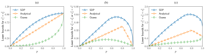
Figure 1: Lower bounds for the errors of the simultaneous measurement of (a) $(X_{1},X_{2})$, (b) $(X_{2},X_{3})$ or $(X_{3},X_{1})$, (c) $(X_{1},X_{2},X_{3})$. The bounds for $(X_{2},X_{3})$ and $(X_{3},X_{1})$ are the same, so they are plotted in the same figure (b). The analytical and Ozawa’s bounds for $(X_{1},X_{2},X_{3})$ are obtained by summing the bounds for all pairs $(X_{j},X_{k})$, while the SDP bound can be directly obtained via the SDP for three observables.

Take $\rho$ and three observables, $X_{1}$, $X_{2}$, $X_{3}$ as

$$\rho=\begin{pmatrix}\frac{p}{2}&0&0\\ 0&1-p&0\\ 0&0&\frac{p}{2}\end{pmatrix},\ X_{1}=\begin{pmatrix}0&1&0\\ 1&0&1\\ 0&1&0\end{pmatrix},$$ (24)

$$X_{2}=\begin{pmatrix}0&-i&0\\ i&0&-i\\ 0&i&0\end{pmatrix},\ X_{3}=\begin{pmatrix}1&0&0\\ 0&0&0\\ 0&0&-1\end{pmatrix}.$$

Here $X_{1}$, $X_{2}$, $X_{3}$ are the spin-1 operators with $[X_{j},X_{k}]\neq 0$ for all $j\neq k$. In this case we have $(\Delta X_{1})^{2}=(\Delta X_{2})^{2}=2-p$, $(\Delta X_{3})^{2}=p$, and

$$c_{12} =\frac{1}{2}\|\sqrt{\rho}[X_{1},X_{2}]\sqrt{\rho}\|_{1}=p,$$ (25)

$$c_{23} =\frac{1}{2}\|\sqrt{\rho}[X_{2},X_{3}]\sqrt{\rho}\|_{1}=\sqrt{p(1-p)},$$

$$c_{31} =\frac{1}{2}\|\sqrt{\rho}[X_{3},X_{1}]\sqrt{\rho}\|_{1}=\sqrt{p(1-p)}.$$

For the simultaneous measurement of $(X_{1},X_{2})$, $(X_{2},X_{3})$, $(X_{3},X_{1})$, the Ozawa’s relation gives

$$\epsilon_{1}^{2}+\epsilon_{2}^{2} \geq\mathcal{E}_{Ozawa}(X_{1},X_{2})=2-p-2\sqrt{1-p},$$ (26)

$$\epsilon_{2}^{2}+\epsilon_{3}^{2} \geq\mathcal{E}_{Ozawa}(X_{2},X_{3})=1-\sqrt{1-p(1-p)},$$

$$\epsilon_{3}^{2}+\epsilon_{1}^{2} \geq\mathcal{E}_{Ozawa}(X_{3},X_{1})=1-\sqrt{1-p(1-p)}.$$

While $\mathcal{E}_{A}$ can be calculated by substituting $\{|u_{q}\rangle\}$ with the eigenvectors of $\sqrt{\rho}[X_{j},X_{k}]\sqrt{\rho}$. Specifically for $(X_{2},X_{3})$, we have $|u_{0}\rangle=(1,\sqrt{2},1)^{T}/2$, $|u_{1}\rangle=(1,-\sqrt{2},1)^{T}/2$, $|u_{2}\rangle=(1,0,-1)^{T}/\sqrt{2}$, which gives

$$\epsilon_{2}^{2}+\epsilon_{3}^{2}\geq\mathcal{E}_{A}(X_{2},X_{3})=\sum_{q=0}^{2}\frac{1}{2}\lambda_{q}\left(\alpha_{q}-\sqrt{\alpha_{q}^{2}-\beta_{q}^{2}}\right)$$ (27)

$$=\frac{2-p}{4}\left(\frac{4-3p}{2-p}-\sqrt{\left(\frac{4-3p}{2-p}\right)^{2}-\left(\frac{4\sqrt{p(1-p)}}{2-p}\right)^{2}}\right)$$

$$=\frac{1}{4}(4-3p-|4-5p|).$$

Similarly for $(X_{1},X_{2})$ and $(X_{3},X_{1})$, we have

$$\epsilon_{1}^{2}+\epsilon_{2}^{2} \geq\mathcal{E}_{A}(X_{1},X_{2})=p,$$ (28)

$$\epsilon_{3}^{2}+\epsilon_{1}^{2} \geq\mathcal{E}_{A}(X_{3},X_{1})=\frac{1}{4}(4-3p-|4-5p|).$$

In Fig. 1, we illustrate the comparisons among the three bounds: (i) $\mathcal{E}_{0}$ that can be computed with SDP; (ii) $\mathcal{E}_{A}$ that can be analytically obtained and (iii) $\mathcal{E}_{Ozawa}$ that obtained from the Ozawa’s relation. It can be seen that for the simultaneous measurement of two observables, we already have $\mathcal{E}_{0}>\mathcal{E}_{A}>\mathcal{E}_{Ozawa}$. While for the simultaneous measurement of three observables, the SDP bound is tighter than the bound obtained by simply adding the results for each pairs of the observables.

VI Tradeoff relations in multiparameter quantum estimation

We next apply the error tradeoff relation to quantum metrology and derive tradeoffs for the precision limits of estimating multiple parameters.

Given a quantum state $\rho_{x}$, where $x=(x_{1},x_{2},\ldots,x_{n})$ are $n$ unknown parameters to be estimated, by performing a POVM, $\{M_{m}\}$, on the state, we can get the measurement result, $m$, with a probability $p_{m}(x)=\mathrm{Tr}(\rho_{x}M_{m})$. For any locally unbiased estimator, $\hat{x}=(\hat{x}_{1},\cdots,\hat{x}_{n})$, the Cramér-Rao bound [30, 31] provides an achievable bound $Cov(\hat{x})\geq\frac{1}{\nu}F_{C}^{-1}$, here $Cov(\hat{x})$ is the covariance matrix for the estimators with the $jk$-th entry given by $Cov(\hat{x})_{jk}=E[(\hat{x}_{j}-x_{j})(\hat{x}_{k}-x_{k})]$, here $E[\cdot]$ denotes the expectation, $\nu$ is the number of the measurement repeated independently, $F_{C}$ is the Fisher information matrix of a single measurement whose $jk$-th entry is given by $(F_{C})_{jk}=\sum_{m}\frac{\partial_{x_{j}}p_{m}(x)\partial_{x_{k}}p_{m}(x)}{p_{m}(x)}$ [31]. Regardless of the choice of the measurement, the covariance matrix is always lower bounded by the quantum Cramér-Rao bound as [32, 33]

$$Cov(\hat{x})\geq\frac{1}{\nu}F_{C}^{-1}\geq\frac{1}{\nu}F_{Q}^{-1},$$ (29)

here $F_{Q}$ is the quantum Fisher information matrix with the $jk$-th entry given by $(F_{Q})_{jk}=\mathrm{Tr}(\rho_{x}\frac{L_{j}L_{k}+L_{k}L_{j}}{2}),$ where $L_{q}$ is the symmetric logarithmic derivative (SLD) corresponding to the parameter $x_{q}$, which satisfies $\partial_{x_{q}}\rho_{x}=\frac{1}{2}(\rho_{x}L_{q}+L_{q}\rho_{x})$. When there is only one parameter, the QCRB can be saturated. In particular it can be saturated with a projective measurement on the eigen-spaces of the SLD, i.e., the SLD is the optimal observable for the estimation of the corresponding parameter.

When there are multiple parameters, the QCRB is in general not saturable since the SLDs typically do not commute with each other. A central task in multi-parameter quantum estimation is to understand the tradeoff induced by such incompatibility [34, 29, 28, 35, 36, 37, 38, 39, 40, 41, 42, 43, 44, 45, 46, 47, 48, 49, 50, 51, 52, 53, 54, 55, 56, 57, 58, 59, 60, 61, 62, 63, 64, 65, 68, 47, 66, 67]. In a recent seminal work [38], by applying Ozawa’s uncertainty relation, Lu and Wang obtained analytical tradeoff relations for the estimation of a pair of parameters. For multiple ($n>2$) parameters, however, if we simply add the tradeoff for each pair of parameters directly, the obtained tradeoff relation is typically loose, which restricts the scope of its applications.

VI.1 Analytical tradeoff relation

From the obtained tradeoff relation in Eq.(8), we can immediately get the tradeoff relation for the estimation of multiple parameters by simply taking the $n$ observables as the $n$ SLDs, $\{L_{1},\cdots,L_{n}\}$. In this case $S_{\text{Re}}$ equals to the quantum Fisher information matrix, $F_{Q}$. Again for any POVM, $\{M_{m}\}$, we use $\{F_{j}=\sum_{m}f_{j}(m)V_{m}\}$ to approximate the SLDs, here $V_{m}$, as defined previously, is the projective measurement on the extended space that reduces to $M_{m}$ on the system. Since the error-tradeoff relation in Eq.(8) holds for any choice of $\{f_{j}(m)\}$, specifically we can choose

$$f_{j}(m)=\frac{1}{2}\frac{\mathrm{Tr}[\{L_{j}\otimes I,\rho_{x}\otimes\sigma\}V_{m}]}{\mathrm{Tr}[(\rho_{x}\otimes\sigma)V_{m}]}=\frac{\partial_{x_{j}}p_{m}(x)}{p_{m}(x)},$$ (30)

where $p_{m}(x)=\mathrm{Tr}[(\rho_{x}\otimes\sigma)V_{m}]=\mathrm{Tr}[\rho_{x}M_{m}]$. This choice actually minimizes $\epsilon_{j}^{2}=\mathrm{Tr}\left[(F_{j}-L_{j}\otimes I)^{2}\left(\rho_{x}\otimes\sigma\right)\right]$ under the given measurement(see Appendix H). With this choice we have $Q_{\text{Re}}=F_{Q}-F_{C}$, Eq.(8) then becomes

$$\mathrm{Tr}[F_{Q}^{-1}(F_{Q}-F_{C})]\geq\left(\sqrt{\|F_{Q}^{-\frac{1}{2}}\tilde{S}_{\text{Im}}F_{Q}^{-\frac{1}{2}}\|_{F}+1}-1\right)^{2},$$ (31)

where $\tilde{S}_{\text{Im}}=\sum_{q}\tilde{S}_{u_{q},\text{Im}}$ with each $\tilde{S}_{u_{q},\text{Im}}$ equals to either $S_{u_{q},\text{Im}}$ or $S_{u_{q},\text{Im}}^{T}$, here $(S_{u_{q},\text{Im}})_{jk}=\frac{1}{2i}\langle u_{q}|(\sqrt{\rho_{x}}\otimes|\xi_{0}\rangle\langle\xi_{0}|)([L_{j},L_{k}]\otimes I)(\sqrt{\rho_{x}}\otimes|\xi_{0}\rangle\langle\xi_{0}|)|u_{q}\rangle$ with $\{|u_{q}\rangle\}$ as any set of vectors that satisfies $\sum_{q}|u_{q}\rangle\langle u_{q}|=I$. This then provides an upper bound on the achievable classical Fisher information matrix as

$$\mathrm{Tr}[F_{Q}^{-1}F_{C}]\leq n-\left(\sqrt{\|F_{Q}^{-\frac{1}{2}}\tilde{S}_{\text{Im}}F_{Q}^{-\frac{1}{2}}\|_{F}+1}-1\right)^{2}.$$ (32)

VI.2 Tradeoff relation with SDP

For the estimation of multiple parameters encoded in a quantum state, $\rho_{x}$, with $x=(x_{1},\cdots,x_{n})$, we can simply replace $\mathbb{X}$ in Eq.(12) with $\mathbb{L}=\begin{pmatrix}L_{1}&L_{2}&\cdots&L_{n}\end{pmatrix}^{\dagger}$ with $L_{q}$ as the SLD for the parameter $x_{q}$. With the optimal choice of $f_{j}(m)$, we have $Q_{\text{Re}}=F_{Q}-F_{C}$. The bound, $\mathcal{E}\geq\mathcal{E}_{0}$ then gives

$$\mathcal{E}=\mathrm{Tr}(WQ)=\mathrm{Tr}(WQ_{\text{Re}})=\mathrm{Tr}[W(F_{Q}-F_{C})]\geq\mathcal{E}_{0},$$ (33)

where $\mathrm{Tr}(WQ_{\text{Im}})=\mathrm{Tr}(W^{\frac{1}{2}}Q_{\text{Im}}W^{\frac{1}{2}})=0$ since $Q_{\text{Im}}$ is anti-symmetric, and

$$\mathcal{E}_{0}=\min_{\mathbb{S},\{R_{j}\}_{j=1}^{n}} \mathrm{Tr}\left[(W\otimes\rho_{x})(\mathbb{S}-\mathbb{R}\mathbb{L}^{\dagger}-\mathbb{L}\mathbb{R}^{\dagger}+\mathbb{L}\mathbb{L}^{\dagger})\right]$$ (34)

subject to $$\mathbb{S}_{jk}=\mathbb{S}_{kj}=\mathbb{S}_{jk}^{\dagger},\ \forall j,k$$

$$R_{j}=R_{j}^{\dagger},\ \forall j$$

$$\begin{pmatrix}I&\mathbb{R}^{\dagger}\\ \mathbb{R}&\mathbb{S}\end{pmatrix}\geq 0.$$

We can take a reparameterization with $\tilde{x}=F_{Q}^{-\frac{1}{2}}x$ such that $\tilde{F}_{Q}=I$. In this case $\mathrm{Tr}[I\otimes\rho_{x})\tilde{\mathbb{L}}\tilde{\mathbb{L}}^{\dagger}]=\mathrm{Tr}(\tilde{F}_{Q})=n$, where $\tilde{\mathbb{L}}=\begin{pmatrix}\tilde{L}_{1}&\tilde{L}_{2}&\cdots&\tilde{L}_{n}\end{pmatrix}^{\dagger}$ with $\tilde{L}_{j}=\sum_{k}(F_{Q}^{-\frac{1}{2}})_{jk}L_{k}$. We then let $W=I$ and get an upper bound for $\mathrm{Tr}(\tilde{F}_{C})=\mathrm{Tr}(F_{Q}^{-1}F_{C})$ as

$$\mathrm{Tr}(F_{Q}^{-1}F_{C})\leq\max_{\mathbb{S},\{R_{j}\}_{j=1}^{n}} \mathrm{Tr}\left[(I\otimes\rho_{x})(-\mathbb{S}+\mathbb{R}\tilde{\mathbb{L}}^{\dagger}+\tilde{\mathbb{L}}\mathbb{R}^{\dagger})\right]$$ (35)

subject to $$\mathbb{S}_{jk}=\mathbb{S}_{kj}=\mathbb{S}_{jk}^{\dagger},\ \forall j,k$$

$$R_{j}=R_{j}^{\dagger},\ \forall j$$

$$\begin{pmatrix}I&\mathbb{R}^{\dagger}\\ \mathbb{R}&\mathbb{S}\end{pmatrix}\geq 0.$$

This resembles the Nagaoka-Hayashi bound [43] but are different. The Nagaoka-Hayashi bound quantifies $\mathrm{Tr}[WCov(\hat{x})]$, where $\hat{x}$ is required to be locally unbiased estimators to satisfy the classical Cramer-Rao bound, $Cov(\hat{x})\geq\frac{1}{\nu}F_{C}^{-1}$. The Nagaoka-Hayashi bound thus has the locally unbiased condition included in the constraints. And it does not have a direct connection to the approximation of the observables, which is reflected in the fact that its objective function does not contain the SLDs. While the bound here quantifies directly the relation between $F_{Q}$ and $F_{C}$, without the intermediate step of estimators, it thus does not have the locally unbiased condition in the constraints. The appearance of the SLD operators in the objective function reflects the intrinsic connection to observable approximation absent in the Nagaoka-Hayashi bound.

VI.3 Tighter tradeoff relation for two parameters

For the estimation of two parameters, we can obtain an analytical bound from Eq.(16) by replacing $(X_{1},X_{2})$ with $(L_{1},L_{2})$, which gives

$$w_{1}[(F_{Q})_{11}-(F_{C})_{11}]+w_{2}[(F_{Q})_{22}-(F_{C})_{22}]$$ (36)

$$\geq \sum_{q}\frac{\lambda_{q}}{2}\left(\alpha_{q}-\sqrt{\alpha_{q}^{2}-\beta_{q}^{2}}\right),$$

where $\lambda_{q}=\langle u_{q}|\rho_{x}|u_{q}\rangle$, $\alpha_{q}$ and $\beta_{q}$ are given as

$$\alpha_{q} =w_{1}(\Delta_{|\phi_{q}\rangle}L_{1})^{2}+w_{2}(\Delta_{|\phi_{q}\rangle}L_{2})^{2},$$ (37)

$$\beta_{q} =i\sqrt{w_{1}w_{2}}\langle\phi_{q}|[L_{1},L_{2}]|\phi_{q}\rangle,$$

here $|\phi_{q}\rangle=\frac{\sqrt{\rho_{x}}|u_{q}\rangle}{\sqrt{\langle u_{q}|\rho_{x}|u_{q}\rangle}}$ and $\Delta_{|\phi_{q}\rangle}L_{1/2}$ denotes the standard deviation of the SLD $L_{1/2}$ on the state $|\phi_{q}\rangle$. By choosing $\{|u_{q}\rangle\}$ as the eigenvectors of $\sqrt{\rho_{x}}[L_{1},L_{2}]\sqrt{\rho_{x}}$, as shown in Appendix F.2, Eq.(36) is tighter than Lu-Wang bound for mixed states [38], which is based on Ozawa’s relation.

VII Summary

We provided approaches that can lead to tradeoff relations for the approximation of an arbitrary number of observables with a single measurement and tightened the existing analytical bounds in the case of two observables. Each of these bounds has its own advantages and disadvantages:

1. $\mathrm{Tr}(S_{\text{Re}}^{-1}Q_{\text{Re}})\geq\left(\sqrt{\|S_{\text{Re}}^{-\frac{1}{2}}\tilde{S}_{\text{Im}}S_{\text{Re}}^{-\frac{1}{2}}\|_{F}+1}-1\right)^{2}$. This is an analytical bound that works for arbitrary number of observables. For pure state it is always tighter than the bound obtained from the simple summation of the Ozawa’s relation when the number of observables is larger than 4. For mixed state, it depends on choices of $\{|u_{q}\rangle\}$ with $|u_{q}\rangle\langle u_{q}|=I$. Any choice of $\{|u_{q}\rangle\}$ leads to a valid bound but there is not yet a systematic way to find the optimal choice.

2. $\mathcal{E}=\mathrm{Tr}(WQ)\geq\mathcal{E}_{0}$ where $\mathcal{E}_{0}$ can be computed efficiently with semidefinite programming as

   $$\mathcal{E}_{0}=\min_{\mathbb{S},\{R_{j}\}_{j=1}^{n}} \mathrm{Tr}\left[(W\otimes\rho)(\mathbb{S}-\mathbb{R}\mathbb{X}^{\dagger}-\mathbb{X}\mathbb{R}^{\dagger}+\mathbb{X}\mathbb{X}^{\dagger})\right]$$ (38)

   subject to $$\mathbb{S}_{jk}=\mathbb{S}_{kj}=\mathbb{S}_{jk}^{\dagger},\ \forall j,k$$

   $$R_{j}=R_{j}^{\dagger},\ \forall j$$

   $$\begin{pmatrix}I&\mathbb{R}^{\dagger}\\ \mathbb{R}&\mathbb{S}\end{pmatrix}\geq 0.$$

   This is the tightest bound and works for arbitrary number of observables. For pure state, this bound is tight and for mixed state it is tighter than the first bound with any choice of $\{|u_{q}\rangle\}$ with $\sum_{q}|u_{q}\rangle\langle u_{q}|=I$. It is always tighter than the bound obtained from the simple summation of the Ozawa’s relation. There is no analytical form for this bound in general case.

3. For a pair of observables $X_{j}$ and $X_{k}$ on $\rho$, we have

   $$w_{j}\epsilon_{j}^{2}+w_{k}\epsilon_{k}^{2}\geq\sum_{q}\frac{\lambda_{q}}{2}\left(\alpha_{q}-\sqrt{\alpha_{q}^{2}-\beta_{q}^{2}}\right),$$ (39)

   where $\lambda_{q}=\langle u_{q}|\rho|u_{q}\rangle$, $|\phi_{q}\rangle=\frac{\sqrt{\rho}|u_{q}\rangle}{\sqrt{\langle u_{q}|\rho|u_{q}\rangle}},$ $\alpha_{q}=w_{j}[\langle\phi_{q}|X_{j}^{2}|\phi_{q}\rangle-\langle\phi_{q}|X_{j}|\phi_{q}\rangle^{2}]+w_{k}[\langle\phi_{q}|X_{k}^{2}|\phi_{q}\rangle-\langle\phi_{q}|X_{k}|\phi_{q}\rangle^{2}]$, $\beta_{q}=i\sqrt{w_{j}w_{k}}\langle\phi_{q}|[X_{j},X_{k}]|\phi_{q}\rangle$. This is an analytical bound that is valid for any choice of $\{|u_{q}\rangle\}$ with $\sum_{q}|u_{q}\rangle\langle u_{q}|=I$. Specifically, if $\{|u_{q}\rangle\}$ is taken as the eigenvectors of $\sqrt{\rho}[X_{j},X_{k}]\sqrt{\rho}$, the bound is always tighter than the Ozawa’s relation for mixed state. It is only for a pair of observables.

Each of the error-tradeoff relations can be directly used to quantify the tradeoff of the precisions for the estimation of multiple parameters in quantum metrology. These tradeoff relations hold under the local measurement which are the measurements performed separately on each copy of $\rho_{x}$. If $p$-local measurements, where the measurements can be performed collectively on at most $p$ copies of $\rho_{x}$, similar tradeoff relations can be obtained by simply replacing $\rho_{x}$ and $\{L_{j}\}$ with $\rho_{x}^{\otimes p}$ and the corresponding SLDs for $\rho_{x}^{\otimes p}$. We provide an example demonstrating the tradeoff relation under collective measurements in Appendix I. This opens the avenue for the studies of the state-dependent measurement uncertainty relations for multiple observables. The connection between the measurement uncertainty relation and the incompatibility of multi-parameter quantum estimation has also been tightened, which is expected to foster studies in both fields.

Appendix A Analytical error-tradeoff relation for multiple observables

In this section we derive the tradeoff relation

$$\mathrm{Tr}(S_{\text{Re}}^{-1}Q_{\text{Re}})\geq\left(\sqrt{\|S_{\text{Re}}^{-\frac{1}{2}}\tilde{S}_{\text{Im}}S_{\text{Re}}^{-\frac{1}{2}}\|_{F}+1}-1\right)^{2}.$$ (40)

Recall given the observables $\{X_{j}|1\leq j\leq n\}$, we can construct $\{F_{j}=\sum_{m}f_{j}(m)V_{m}|1\leq j\leq n\}$ to approximate the observables from a set of projective measurement $\{V_{m}\}$ on the extended space with an acilla. The root-mean-square error of the approximations is given by

$$\epsilon_{j}^{2}=\mathrm{Tr}\left[(F_{j}-X_{j}\otimes I)^{2}\left(\rho\otimes\sigma\right)\right],$$ (41)

where $\sigma=|\xi_{0}\rangle\langle\xi_{0}|$ is a state of the ancilla. We then let

$$\mathcal{A}_{u}= \begin{pmatrix}\langle u|\sqrt{\rho\otimes\sigma}E_{1}\\ \vdots\\ \langle u|\sqrt{\rho\otimes\sigma}E_{n}\\ \langle u|\sqrt{\rho\otimes\sigma}(X_{1}\otimes I)\\ \vdots\\ \langle u|\sqrt{\rho\otimes\sigma}(X_{n}\otimes I)\end{pmatrix}\begin{pmatrix}\langle u|\sqrt{\rho\otimes\sigma}E_{1}\\ \vdots\\ \langle u|\sqrt{\rho\otimes\sigma}E_{n}\\ \langle u|\sqrt{\rho\otimes\sigma}(X_{1}\otimes I)\\ \vdots\\ \langle u|\sqrt{\rho\otimes\sigma}(X_{n}\otimes I)\end{pmatrix}^{\dagger}$$ (42)

$$= \begin{pmatrix}Q_{u}&R_{u}\\ R_{u}^{\dagger}&S_{u}\end{pmatrix}\geq 0,$$

here $E_{j}=F_{j}-X_{j}\otimes I$, $|u\rangle$ is any vector, $Q_{u}$, $R_{u}$, $S_{u}$ are $n\times n$ matrices with the entries given by(note $E_{j}$ and $X_{j}$ are all Hermitian operators)

$$(Q_{u})_{jk} =\langle u|\sqrt{\rho\otimes\sigma}E_{j}E_{k}\sqrt{\rho\otimes\sigma}|u\rangle,$$ (43)

$$(R_{u})_{jk} =\langle u|\sqrt{\rho\otimes\sigma}E_{j}(X_{k}\otimes I)\sqrt{\rho\otimes\sigma}|u\rangle,$$

$$(S_{u})_{jk} =\langle u|\sqrt{\rho\otimes\sigma}(X_{j}\otimes I)(X_{k}\otimes I)\sqrt{\rho\otimes\sigma}|u\rangle.$$

We can write these matrices in terms of the real and imaginary parts as $Q_{u}=Q_{u,\text{Re}}+iQ_{u,\text{Im}}$, $R_{u}=R_{u,\text{Re}}+iR_{u,\text{Im}}$, $S_{u}=S_{u,\text{Re}}+iS_{u,\text{Im}}$, where

$$(Q_{u,\text{Re}})_{jk} =\frac{1}{2}\langle u|\sqrt{\rho\otimes\sigma}\{E_{j},E_{k}\}\sqrt{\rho\otimes\sigma}|u\rangle,$$ (44)

$$(R_{u,\text{Re}})_{jk} =\frac{1}{2}\langle u|\sqrt{\rho\otimes\sigma}\{E_{j},X_{k}\otimes I\}\sqrt{\rho\otimes\sigma}|u\rangle,$$

$$(S_{u,\text{Re}})_{jk} =\frac{1}{2}\langle u|\sqrt{\rho\otimes\sigma}\{X_{j}\otimes I,X_{k}\otimes I\}\sqrt{\rho\otimes\sigma}|u\rangle,$$

and

$$(Q_{u,\text{Im}})_{jk} =\frac{1}{2i}\langle u|\sqrt{\rho\otimes\sigma}[E_{j},E_{k}]\sqrt{\rho\otimes\sigma}|u\rangle,$$ (45)

$$(R_{u,\text{Im}})_{jk} =\frac{1}{2i}\langle u|\sqrt{\rho\otimes\sigma}[E_{j},X_{k}\otimes I]\sqrt{\rho\otimes\sigma}|u\rangle,$$

$$(S_{u,\text{Im}})_{jk} =\frac{1}{2i}\langle u|\sqrt{\rho\otimes\sigma}[X_{j}\otimes I,X_{k}\otimes I]\sqrt{\rho\otimes\sigma}|u\rangle.$$

For any set of $\{|u_{q}\rangle\}$ with $\sum_{q}|u_{q}\rangle\langle u_{q}|=I$, we can obtain a corresponding set of $\{\mathcal{A}_{u_{q}}\}$. We then let $\tilde{{\mathcal{A}}}=\sum_{q}\tilde{\mathcal{A}}_{u_{q}}$ with each $\tilde{\mathcal{A}}_{u_{q}}$ equals to either $\mathcal{A}_{u_{q}}$ or $\mathcal{A}_{u_{q}}^{T}$. Since $\mathcal{A}_{u_{q}}\geq 0$, and $\mathcal{A}_{u_{q}}^{T}\geq 0$, we have

$$\tilde{\mathcal{A}}=\sum_{q}\tilde{\mathcal{A}}_{u_{q}}=\begin{pmatrix}\tilde{Q}&\tilde{R}\\ \tilde{R}^{\dagger}&\tilde{S}\end{pmatrix}\geq 0,$$ (46)

where $\tilde{Q}=\sum_{q}\tilde{Q}_{u_{q}}$, $\tilde{R}=\sum_{q}\tilde{R}_{u_{q}}$, $\tilde{S}=\sum_{q}\tilde{S}_{u_{q}}$ with each $(\tilde{Q}_{u_{q}},\tilde{R}_{u_{q}},\tilde{S}_{u_{q}})$ equals to either $(Q_{u_{q}},R_{u_{q}},S_{u_{q}})$ or $(\bar{Q}_{u_{q}},\bar{R}_{u_{q}},\bar{S}_{u_{q}})$, here $\bar{M}=M_{\text{Re}}-iM_{\text{Im}}$. We assume $\tilde{S}$ is nonsingular, which means $\{X_{j}\}$ are linearly independent.

Since $\tilde{\mathcal{A}}\geq 0$, with the Schur complement, we have

$$\tilde{Q}-\tilde{R}\tilde{S}^{-1}\tilde{R}^{\dagger}\geq 0.$$ (47)

This can be rewritten as $\tilde{Q}-(i\tilde{R})\tilde{S}^{-1}(i\tilde{R})^{\dagger}\geq 0$, which is the Schur complement of

$$\tilde{\mathcal{B}}=\begin{pmatrix}\tilde{Q}&i\tilde{R}\\ (i\tilde{R})^{\dagger}&\tilde{S}\end{pmatrix}.$$ (48)

Since $\tilde{Q}-(i\tilde{R})\tilde{S}^{-1}(i\tilde{R})^{\dagger}\geq 0$ and $\tilde{S}>0$, we then have $\tilde{\mathcal{B}}\geq 0$. This implies $\tilde{\mathcal{B}}_{\text{Re}}=\frac{1}{2}(\tilde{\mathcal{B}}+\tilde{\mathcal{B}}^{T})\geq 0$, which can be written as

$$\tilde{\mathcal{B}}_{\text{Re}}=\begin{pmatrix}\tilde{Q}_{\text{Re}}&-\tilde{R}_{\text{Im}}\\ -\tilde{R}_{\text{Im}}^{T}&\tilde{S}_{\text{Re}}\end{pmatrix}\geq 0.$$ (49)

With the Schur complement of $\tilde{\mathcal{B}}_{\text{Re}}$ we have

$$\tilde{Q}_{\text{Re}}-\tilde{R}_{\text{Im}}\tilde{S}_{\text{Re}}^{-1}\tilde{R}_{\text{Im}}^{T}\geq 0.$$ (50)

This implies

$$\tilde{S}_{\text{Re}}^{-\frac{1}{2}}\tilde{Q}_{\text{Re}}\tilde{S}_{\text{Re}}^{-\frac{1}{2}}-\tilde{S}_{\text{Re}}^{-\frac{1}{2}}\tilde{R}_{\text{Im}}\tilde{S}_{\text{Re}}^{-1}\tilde{R}_{\text{Im}}^{T}\tilde{S}_{\text{Re}}^{-\frac{1}{2}}\geq 0,$$ (51)

thus

$$\mathrm{Tr}(\tilde{S}_{\text{Re}}^{-\frac{1}{2}}\tilde{Q}_{\text{Re}}\tilde{S}_{\text{Re}}^{-\frac{1}{2}}) \geq\mathrm{Tr}(\tilde{S}_{\text{Re}}^{-\frac{1}{2}}\tilde{R}_{\text{Im}}\tilde{S}_{\text{Re}}^{-1}\tilde{R}_{\text{Im}}^{T}\tilde{S}_{\text{Re}}^{-\frac{1}{2}})$$ (52)

$$=\|\tilde{S}_{\text{Re}}^{-\frac{1}{2}}\tilde{R}_{\text{Im}}\tilde{S}_{\text{Re}}^{-\frac{1}{2}}\|_{F}^{2},$$

where $\|\cdot\|_{F}$ is the Frobenius norm. Here the right side of the inequality depends on $\tilde{R}_{\text{Im}}$, which depends on the choice of the measurement. To get rid of $\tilde{R}_{\text{Im}}$, we use the fact that $[F_{j},F_{k}]=0$ since they are constructed from the same projective measurement. $[F_{j},F_{k}]=0$ can be rewritten as $[E_{j}+X_{j}\otimes I,E_{k}+X_{k}\otimes I]=0$, which can be expanded as

$$[E_{j},E_{k}]+[E_{j},X_{k}\otimes I]+[X_{j}\otimes I,E_{k}]+[X_{j}\otimes I,X_{k}\otimes I]=0.$$ (53)

From which we have $Q_{u_{q},\text{Im}}+R_{u_{q},\text{Im}}-R_{u_{q},\text{Im}}^{T}+S_{u_{q},\text{Im}}=0$. Since $(\tilde{Q}_{u_{q}},\tilde{R}_{u_{q}},\tilde{S}_{u_{q}})$ equal to either $(Q_{u_{q}},R_{u_{q}},S_{u_{q}})$ or $(\bar{Q}_{u_{q}},\bar{R}_{u_{q}},\bar{S}_{u_{q}})$, $(\tilde{Q}_{u_{q},\text{Im}},\tilde{R}_{u_{q},\text{Im}},\tilde{S}_{u_{q},\text{Im}})$ then equal to either $(Q_{u_{q},\text{Im}},R_{u_{q},\text{Im}},S_{u_{q},\text{Im}})$ or $(-Q_{u_{q},\text{Im}},-R_{u_{q},\text{Im}},-S_{u_{q},\text{Im}})$. In either case $\tilde{Q}_{u_{q},\text{Im}}+\tilde{R}_{u_{q},\text{Im}}-\tilde{R}_{u_{q},\text{Im}}^{T}+\tilde{S}_{u_{q},\text{Im}}=0$ holds, thus $\sum_{q}(\tilde{Q}_{u_{q},\text{Im}}+\tilde{R}_{u_{q},\text{Im}}-\tilde{R}_{u_{q},\text{Im}}^{T}+\tilde{S}_{u_{q},\text{Im}})=0$. This can be written as

$$\tilde{Q}_{\text{Im}}+\tilde{R}_{\text{Im}}-\tilde{R}_{\text{Im}}^{T}+\tilde{S}_{\text{Im}}=0.$$ (54)

By multiplying $\tilde{S}_{\text{Re}}^{-\frac{1}{2}}$ from both left and right, we have $\hat{Q}_{\text{Im}}+\hat{R}_{\text{Im}}-\hat{R}_{\text{Im}}^{T}+\hat{S}_{\text{Im}}=0$, which can be equivalently written as

$$\hat{S}_{\text{Im}}=-\hat{Q}_{\text{Im}}-\hat{R}_{\text{Im}}+\hat{R}_{\text{Im}}^{T},$$ (55)

where $\hat{\Box}=\tilde{S}_{\text{Re}}^{-\frac{1}{2}}\tilde{\Box}\tilde{S}_{\text{Re}}^{-\frac{1}{2}}$. Applying the triangle inequality we get

$$\|\hat{S}_{\text{Im}}\|_{F}\leq\|\hat{Q}_{\text{Im}}\|_{F}+\|\hat{R}_{\text{Im}}\|_{F}+\|\hat{R}_{\text{Im}}^{T}\|_{F}.$$ (56)

Note that Eq.(52) can be rewritten as $\|\hat{R}_{\text{Im}}^{T}\|_{F}^{2}=\|\hat{R}_{\text{Im}}\|_{F}^{2}\leq\mathrm{Tr}(\hat{Q}_{\text{Re}})$, and from $\hat{Q}\geq 0$ we have

$$\mathrm{Tr}(\hat{Q}_{\text{Re}})\geq\|\hat{Q}_{\text{Im}}\|_{1}\geq\|\hat{Q}_{\text{Im}}\|_{F}.$$ (57)

Combining these inequalities we then have

$$\|\hat{S}_{\text{Im}}\|_{F} \leq\|\hat{Q}_{\text{Im}}\|_{F}+\|\hat{R}_{\text{Im}}\|_{F}+\|\hat{R}_{\text{Im}}^{T}\|_{F}$$ (58)

$$\leq\mathrm{Tr}(\hat{Q}_{\text{Re}})+2\sqrt{\mathrm{Tr}(\hat{Q}_{\text{Re}})}.$$

This leads to the bound on $\mathrm{Tr}(\hat{Q}_{\text{Re}})$ as

$$\mathrm{Tr}(\hat{Q}_{\text{Re}})\geq\left(\sqrt{\|\hat{S}_{\text{Im}}\|_{F}+1}-1\right)^{2},$$ (59)

which can be equivalently written as

$$\mathrm{Tr}(S_{\text{Re}}^{-1}Q_{\text{Re}})\geq\left(\sqrt{\|S_{\text{Re}}^{-\frac{1}{2}}\tilde{S}_{\text{Im}}S_{\text{Re}}^{-\frac{1}{2}}\|_{F}+1}-1\right)^{2}.$$ (60)

Appendix B Error-tradeoff relation with semidefinite programming

Recall that given a set of observables $\{X_{j}\}_{j=1}^{n}$ in Hilbert space $\mathcal{H}_{S}$, we can construct $\{F_{j}=\sum_{m}f_{j}(m)V_{m}\}_{j=1}^{n}$ to approximate the observables from a set of projective measurement $\{V_{m}\}$ on the extended space $\mathcal{H}_{S}\otimes\mathcal{H}_{A}$. We denote the weighted root-mean-square error of the approximations as

$$\mathcal{E}=\sum_{j=1}^{n}w_{j}\epsilon_{j}^{2}=\sum_{j=1}^{n}w_{j}\mathrm{Tr}[(\rho\otimes\sigma)(F_{j}-X_{j}\otimes I)^{2}],$$ (61)

where $\rho\in\mathcal{H}_{S}$ is the state of the system and $\sigma=|\xi_{0}\rangle\langle\xi_{0}|\in\mathcal{H}_{A}$ is the state of the ancilla. To formularize the minimization of $\mathcal{E}$ over all choices of $\{F_{j}\}_{j=1}^{n}$, we first define an $n\times n$ Hermitian matrix $Q$, whose $jk$-th element is given by

$$Q_{jk}= \mathrm{Tr}\left[(\rho\otimes\sigma)(F_{j}-X_{j}\otimes I)(F_{k}-X_{k}\otimes I)\right]$$ (62)

$$= \mathrm{Tr}\left[(\rho\otimes\sigma)F_{j}F_{k}\right]-\mathrm{Tr}\left[(\rho\otimes\sigma)F_{j}(X_{k}\otimes I)\right]$$

$$-\mathrm{Tr}\left[(\rho\otimes\sigma)(X_{j}\otimes I)F_{k}\right]$$

$$+\mathrm{Tr}\left[(\rho\otimes\sigma)(X_{j}\otimes I)(X_{k}\otimes I)\right]$$

$$= \mathrm{Tr}\left[\rho\sum_{m}f_{j}(m)M_{m}f_{k}(m)\right]-\mathrm{Tr}\left(\rho R_{j}X_{k}\right)$$

$$-\mathrm{Tr}\left(\rho X_{j}R_{k}\right)+\mathrm{Tr}\left(\rho X_{j}X_{k}\right),$$

where $R_{j}=(I\otimes\langle\xi_{0}|)F_{j}(I\otimes|\xi_{0}\rangle)=\sum_{m}f_{j}(m)M_{m}$ for $1\leq j\leq n$ are Hermitian matrices in $\mathcal{H}_{S}$, $\{M_{m}=(I\otimes\langle\xi_{0}|)V_{m}(I\otimes|\xi_{0}\rangle)\}$ forms a POVM. We denote $\mathbb{S}_{jk}=\sum_{m}f_{j}(m)M_{m}f_{k}(m)$, $\mathbb{R}=\begin{pmatrix}R_{1}&R_{2}&\cdots&R_{n}\end{pmatrix}^{\dagger}$ and $\mathbb{X}=\begin{pmatrix}X_{1}&X_{2}&\cdots&X_{n}\end{pmatrix}^{\dagger}$, the Hermitian matrix $Q$ can then be written as $Q=\mathrm{Tr}_{S}\left[(I_{n}\otimes\rho)(\mathbb{S}-\mathbb{R}\mathbb{X}^{\dagger}-\mathbb{X}\mathbb{R}^{\dagger}+\mathbb{X}\mathbb{X}^{\dagger})\right]$, and

$$\mathcal{E}= \mathrm{Tr}(WQ)=\mathrm{Tr}\left[(W\otimes\rho)(\mathbb{S}-\mathbb{R}\mathbb{X}^{\dagger}-\mathbb{X}\mathbb{R}^{\dagger}+\mathbb{X}\mathbb{X}^{\dagger})\right],$$ (63)

where $\mathbb{S}$ is a $n\times n$ block matrix with the $jk$-th block as $\mathbb{S}_{jk}$, which is itself a Hermitian operator,$W\geq 0$ is a weighted matrix, which is typically taken as $W=diag\{w_{1},\cdots,w_{n}\}$ , but it can also be taken as a general positive semidefinite matrix.

We now show that for the defined $\mathbb{S}$ and $\mathbb{R}$, we have $\mathbb{S}\geq\mathbb{R}\mathbb{R}^{\dagger}$. Since $\mathbb{S}$ and $\mathbb{R}\mathbb{R}^{\dagger}$ are $nd_{s}\times nd_{s}$ matrices, where $d_{S}$ is the dimension of $\mathcal{H}_{S}$, $\mathbb{S}\geq\mathbb{R}\mathbb{R}^{\dagger}$ is equivalent to $b^{\dagger}(\mathbb{S}-\mathbb{R}\mathbb{R}^{\dagger})b\geq 0$ for any $nd_{S}\times 1$ vector $b$.

For any $nd_{S}\times 1$ vector, $b$, we can write $b^{\dagger}$ as $b^{\dagger}=\begin{pmatrix}\langle b_{1}|&\langle b_{2}|&\cdots&\langle b_{n}|\end{pmatrix}$ with $\{\langle b_{j}|\}_{j=1}^{n}$ being $d_{S}$-dimensional row vectors. We then have

$$b^{\dagger}\mathbb{S}b-b^{\dagger}\mathbb{R}\mathbb{R}^{\dagger}b=\sum_{j,k}\langle b_{j}|(\mathbb{S}_{jk}-R_{j}R_{k})|b_{k}\rangle$$ (64)

$$= \sum_{j,k}\langle b_{j}|\left[\sum_{m}f_{j}(m)M_{m}f_{k}(m)-\left(\sum_{m}f_{j}(m)M_{m}\right)\left(\sum_{l}f_{k}(l)M_{l}\right)\right]|b_{k}\rangle$$

$$= \sum_{m}\left(\sum_{j}\langle b_{j}|f_{j}(m)\right)M_{m}\left(\sum_{k}f_{k}(m)|b_{k}\rangle\right)-\left[\sum_{m}\left(\sum_{j}\langle b_{j}|f_{j}(m)\right)M_{m}\right]\left[\sum_{l}M_{l}\left(\sum_{k}f_{k}(l)|b_{k}\rangle\right)\right]$$

$$= \sum_{m}\left[\sum_{j}\langle b_{j}|f_{j}(m)-\sum_{l}\left(\sum_{j}\langle b_{j}|f_{j}(l)\right)M_{l}\right]M_{m}\left[\sum_{k}f_{k}(m)|b_{k}\rangle-\sum_{l}M_{l}\left(\sum_{k}f_{k}(l)|b_{k}\rangle\right)\right]$$

$$= \sum_{m}V_{m}^{\dagger}M_{m}V_{m}\geq 0,$$

where $V_{m}=\sum_{k}f_{k}(m)|b_{k}\rangle-\sum_{l}M_{l}\left(\sum_{k}f_{k}(l)|b_{k}\rangle\right)=\sum_{j}f_{j}(m)|b_{j}\rangle-\sum_{l}M_{l}\left(\sum_{j}f_{j}(l)|b_{j}\rangle\right)$. We thus have $\mathbb{S}\geq\mathbb{R}\mathbb{R}^{\dagger}$.

Denote $\{R_{j}^{\star}\}_{j=1}^{n}$ and $\mathbb{S}^{\star}$ as the optimal operators that gives the minimal error, $\mathcal{E}^{\star}$, we then have

$$\mathcal{E}\geq\mathcal{E}^{\star} =\mathrm{Tr}\left[(W\otimes\rho)(\mathbb{S}^{\star}-\mathbb{R}^{\star}\mathbb{X}^{\dagger}-\mathbb{X}\mathbb{R}^{\star\dagger}+\mathbb{X}\mathbb{X}^{\dagger})\right]$$ (65)

$$\geq\min_{\mathbb{S}}\left\{\mathrm{Tr}\left[(W\otimes\rho)(\mathbb{S}-\mathbb{R}^{\star}\mathbb{X}^{\dagger}-\mathbb{X}\mathbb{R}^{\star\dagger}+\mathbb{X}\mathbb{X}^{\dagger})\right]|\mathbb{S}_{jk}=\mathbb{S}_{jk}^{\dagger}=\mathbb{S}_{kj},\mathbb{S}\geq\mathbb{R}^{\star}\mathbb{R}^{\star\dagger}\right\}$$

$$\geq\min_{\mathbb{S},\{R_{j}\}_{j=1}^{n}}\left\{\mathrm{Tr}\left[(W\otimes\rho)(\mathbb{S}-\mathbb{R}\mathbb{X}^{\dagger}-\mathbb{X}\mathbb{R}^{\dagger}+\mathbb{X}\mathbb{X}^{\dagger})\right]|\mathbb{S}_{jk}=\mathbb{S}_{jk}^{\dagger}=\mathbb{S}_{kj},\mathbb{S}\geq\mathbb{R}\mathbb{R}^{\dagger},R_{j}=R_{j}^{\dagger}\right\}.$$

And the minimization can be formulated as a semidefinite programming as

$$\mathcal{E}_{0}=\min_{\mathbb{S},\{R_{j}\}_{j=1}^{n}} \mathrm{Tr}\left[(W\otimes\rho)(\mathbb{S}-\mathbb{R}\mathbb{X}^{\dagger}-\mathbb{X}\mathbb{R}^{\dagger}+\mathbb{X}\mathbb{X}^{\dagger})\right]$$ (66)

subject to $$\mathbb{S}_{jk}=\mathbb{S}_{kj}=\mathbb{S}_{jk}^{\dagger},\ \forall j,k$$

$$R_{j}=R_{j}^{\dagger},\ \forall j$$

$$\begin{pmatrix}I&\mathbb{R}^{\dagger}\\ \mathbb{R}&\mathbb{S}\end{pmatrix}\geq 0.$$

Appendix C Comparison of the SDP and analytical bound

In this section we show that the bound $\mathcal{E}_{0}$ is tighter than the analytical bounds with any choice of $\{|u_{q}\rangle\}$.

Recall that for any vector $|u\rangle$ in $\mathcal{H}_{S}\otimes\mathcal{H}_{A}$, we have

$$\mathcal{A}_{u}= \begin{pmatrix}\langle u|\sqrt{\rho\otimes\sigma}(F_{1}-X_{1}\otimes I)\\ \vdots\\ \langle u|\sqrt{\rho\otimes\sigma}(F_{n}-X_{n}\otimes I)\\ \langle u|\sqrt{\rho\otimes\sigma}(X_{1}\otimes I)\\ \vdots\\ \langle u|\sqrt{\rho\otimes\sigma}(X_{n}\otimes I)\end{pmatrix}\begin{pmatrix}\langle u|\sqrt{\rho\otimes\sigma}(F_{1}-X_{1}\otimes I)\\ \vdots\\ \langle u|\sqrt{\rho\otimes\sigma}(F_{n}-X_{n}\otimes I)\\ \langle u|\sqrt{\rho\otimes\sigma}(X_{1}\otimes I)\\ \vdots\\ \langle u|\sqrt{\rho\otimes\sigma}(X_{n}\otimes I)\end{pmatrix}^{\dagger}$$ (67)

$$= \begin{pmatrix}Q_{u}&D_{u}\\ D_{u}^{\dagger}&J_{u}\end{pmatrix}\geq 0,$$

where $Q_{u}$, $D_{u}$, $J_{u}$ are $n\times n$ matrices with the $jk$-th elements given by

$$(Q_{u})_{jk} =\langle u|\sqrt{\rho\otimes\sigma}(F_{j}-X_{j}\otimes I)(F_{k}-X_{k}\otimes I)\sqrt{\rho\otimes\sigma}|u\rangle,$$ (68)

$$(D_{u})_{jk} =\langle u|\sqrt{\rho\otimes\sigma}(F_{j}-X_{j}\otimes I)(X_{k}\otimes I)\sqrt{\rho\otimes\sigma}|u\rangle,$$

$$(J_{u})_{jk} =\langle u|\sqrt{\rho\otimes\sigma}(X_{j}\otimes I)(X_{k}\otimes I)\sqrt{\rho\otimes\sigma}|u\rangle.$$

Note that $[F_{j},F_{k}]=0$, which gives

$$(Q_{u}+D_{u}+D_{u}^{\dagger}+J_{u})_{jk}=(Q_{u}+D_{u}+D_{u}^{\dagger}+J_{u})_{kj},$$ (69)

i.e., the matrix $Q_{u}+D_{u}+D_{u}^{\dagger}+J_{u}$ is real symmetric. For any set of vectors $\{|u_{q}\rangle\}$ that satistifies $\sum_{q}|u_{q}\rangle\langle u_{q}|=I$, we have $Q=\sum_{q}Q_{u_{q}}$. Together with Eq.(67) and Eq.(69), we can write the bound as a minimization,

$$\mathcal{E}_{u}=\min_{\{F_{j}\}} \mathrm{Tr}[WQ]=\sum_{q}\mathrm{Tr}[WQ_{u_{q}}]$$ (70)

subject to $$\begin{pmatrix}Q_{u_{q}}&D_{u_{q}}\\ D_{u_{q}}^{\dagger}&J_{u_{q}}\end{pmatrix}\geq 0,\forall q$$

$$Q_{u_{q}}+D_{u_{q}}+D_{u_{q}}^{\dagger}+J_{u_{q}}\ \text{real symmetric},\forall q.$$

$\mathcal{E}_{u}$ is tighter than any analytical bounds based on it, unless any other potential constraints could be introduced. In particular it is tighter than the analytical bound obtained in Appendix A. We will then show $\mathcal{E}_{0}$ is tighter than $\mathcal{E}_{u}$ for any $\{|u_{q}\rangle\}$.

We first formulate $\mathcal{E}_{u}$ as a semidefinite programming for a fixed $\{|u_{q}\rangle\}$, then show that $\mathcal{E}_{0}\geq\mathcal{E}_{u}$ for any $\{|u_{q}\rangle\}$. First note that since $\sigma=|\xi_{0}\rangle\langle\xi_{0}|$, we have

$$\begin{aligned} &\sqrt{\rho\otimes\sigma}|u_{q}\rangle\langle u_{q}|\sqrt{\rho\otimes\sigma}\\ &=(\sqrt{\rho}\otimes|\xi_{0}\rangle)(I\otimes\langle\xi_{0}|)|u_{q}\rangle\langle u_{q}|(I\otimes|\xi_{0}\rangle)(\sqrt{\rho}\otimes\langle\xi_{0}|)\\ &=(\sqrt{\rho}\otimes|\xi_{0}\rangle)\tilde{\rho}(\sqrt{\rho}\otimes\langle\xi_{0}|)\\ &=\sqrt{\rho}\tilde{\rho}\sqrt{\rho}\otimes|\xi_{0}\rangle\langle\xi_{0}|\\ &=\rho_{u_{q}}\otimes\sigma,\end{aligned}$$ (71)

here $\tilde{\rho}=(I\otimes\langle\xi_{0}|)|u_{q}\rangle\langle u_{q}|(I\otimes|\xi_{0}\rangle)$ and $\rho_{u_{q}}=\sqrt{\rho}\tilde{\rho}\sqrt{\rho}$ . We note that $\sum_{q}\rho_{u_{q}}=\rho$, and each $\rho_{u_{q}}$ is unnormalized with rank equal to 1. With $\mathbb{S}_{jk}=\sum_{m}f_{j}(m)M_{m}f_{k}(m)$, $\mathbb{R}=\begin{pmatrix}R_{1}&R_{2}&\cdots&R_{n}\end{pmatrix}^{\dagger}$ and $\mathbb{X}=\begin{pmatrix}X_{1}&X_{2}&\cdots&X_{n}\end{pmatrix}^{\dagger}$, we have $Q_{u_{q}}=\mathrm{Tr}_{S}\left[(I_{n}\otimes\rho_{u_{q}})(\mathbb{S}-\mathbb{R}\mathbb{X}^{\dagger}-\mathbb{X}\mathbb{R}^{\dagger}+\mathbb{X}\mathbb{X}^{\dagger})\right]$, $D_{u_{q}}=\mathrm{Tr}_{S}\left[(I_{n}\otimes\rho_{u_{q}})(\mathbb{R}\mathbb{X}^{\dagger}-\mathbb{X}\mathbb{X}^{\dagger})\right]$ and $J_{u_{q}}=\mathrm{Tr}_{S}\left[(I_{n}\otimes\rho_{u_{q}})\mathbb{X}\mathbb{X}^{\dagger}\right]$. With Schur complement, $\begin{pmatrix}Q_{u_{q}}&D_{u_{q}}\\ D_{u_{q}}^{\dagger}&J_{u_{q}}\end{pmatrix}\geq 0$ is equivalent to $Q_{u_{q}}\geq D_{u_{q}}J_{u_{q}}^{-1}D_{u_{q}}^{\dagger}$, which further gives

$$Q_{u_{q}}+(D_{u_{q}}+J_{u_{q}})+(D_{u_{q}}+J_{u_{q}})^{\dagger}-J_{u_{q}}\geq(D_{u_{q}}+J_{u_{q}})J_{u_{q}}^{-1}(D_{u_{q}}+J_{u_{q}})^{\dagger}$$ (72)

$$\Leftrightarrow \mathrm{Tr}_{S}\left[(I_{n}\otimes\rho_{u_{q}})\mathbb{S}\right]\geq\mathrm{Tr}_{S}\left[(I_{n}\otimes\rho_{u_{q}})\mathbb{R}\mathbb{X}^{\dagger}\right]\mathrm{Tr}_{S}\left[(I_{n}\otimes\rho_{u_{q}})\mathbb{X}\mathbb{X}^{\dagger}\right]^{-1}\mathrm{Tr}_{S}\left[(I_{n}\otimes\rho_{u_{q}})\mathbb{R}\mathbb{X}^{\dagger}\right]^{\dagger}$$

$$\Leftrightarrow \begin{pmatrix}\mathrm{Tr}_{S}\left[(I_{n}\otimes\rho_{u_{q}})\mathbb{S}\right]&\mathrm{Tr}_{S}\left[(I_{n}\otimes\rho_{u_{q}})\mathbb{R}\mathbb{X}^{\dagger}\right]\\ \mathrm{Tr}_{S}\left[(I_{n}\otimes\rho_{u_{q}})\mathbb{R}\mathbb{X}^{\dagger}\right]^{\dagger}&\mathrm{Tr}_{S}\left[(I_{n}\otimes\rho_{u_{q}})\mathbb{X}\mathbb{X}^{\dagger}\right]\end{pmatrix}\geq 0$$

$$\Leftrightarrow \mathrm{Tr}_{S}\left[(I_{2}\otimes I_{n}\otimes\rho_{u_{q}})\begin{pmatrix}\mathbb{S}&\mathbb{R}\mathbb{X}^{\dagger}\\ \mathbb{X}\mathbb{R}^{\dagger}&\mathbb{X}\mathbb{X}^{\dagger}\end{pmatrix}\right]\geq 0.$$

Also note that the constraint of $Q_{u_{q}}+D_{u_{q}}+D_{u_{q}}^{\dagger}+J_{u_{q}}$ being real symmetric is equivalent to $\mathrm{Tr}_{S}\left[(I_{n}\otimes\rho_{u_{q}})\mathbb{S}\right]$ being real symmetric. $\mathcal{E}_{u}$ can then be formulated as a semidefinite programming for a fixed $\{|u_{q}\rangle\}$ as

$$\mathcal{E}_{u}=\min_{\mathbb{S},\{R_{j}\}_{j=1}^{n}} \mathrm{Tr}\left[(W\otimes\rho)(\mathbb{S}-\mathbb{R}\mathbb{X}^{\dagger}-\mathbb{X}\mathbb{R}^{\dagger}+\mathbb{X}\mathbb{X}^{\dagger})\right]$$ (73)

subject to $$\mathrm{Tr}_{S}\left[(I_{2}\otimes I_{n}\otimes\rho_{u_{q}})\begin{pmatrix}\mathbb{S}&\mathbb{R}\mathbb{X}^{\dagger}\\ \mathbb{X}\mathbb{R}^{\dagger}&\mathbb{X}\mathbb{X}^{\dagger}\end{pmatrix}\right]\geq 0,\forall q$$

$$\mathrm{Tr}_{S}\left[(I_{n}\otimes\rho_{u_{q}})\mathbb{S}\right]\ \text{real symmetric},\forall q$$

$$R_{j}=R_{j}^{\dagger}.$$

Next we show that $\mathcal{E}_{0}$ is tighter than $\mathcal{E}_{u}$ for any $\{|u_{q}\rangle\}$. Since $\begin{pmatrix}\mathbb{R}\mathbb{R}^{\dagger}&\mathbb{R}\mathbb{X}^{\dagger}\\ \mathbb{X}\mathbb{R}^{\dagger}&\mathbb{X}\mathbb{X}^{\dagger}\end{pmatrix}=\begin{pmatrix}\mathbb{R}\\ \mathbb{X}\end{pmatrix}\begin{pmatrix}\mathbb{R}\\ \mathbb{X}\end{pmatrix}^{\dagger}\geq 0$, combining with the constraint $\mathbb{S}\geq\mathbb{R}\mathbb{R}^{\dagger}$ in $\mathcal{E}_{0}$, we can obtain $\begin{pmatrix}\mathbb{S}&\mathbb{R}\mathbb{X}^{\dagger}\\ \mathbb{X}\mathbb{R}^{\dagger}&\mathbb{X}\mathbb{X}^{\dagger}\end{pmatrix}\geq 0$, which is stronger than the first constraint in $\mathcal{E}_{u}$. From the constraint $\mathbb{S}_{jk}=\mathbb{S}_{kj}=\mathbb{S}_{jk}^{\dagger}$, $\forall j,k$ in $\mathcal{E}_{0}$, we can also obtain that $\mathrm{Tr}_{S}\left[(I_{n}\otimes\rho_{u_{q}})\mathbb{S}\right]$ is real symmetric $\forall q$. The semidefinite programming $\mathcal{E}_{0}$ thus has the same objective function but stronger constraints than those in $\mathcal{E}_{u}$, which indicates that $\mathcal{E}_{0}\geq\mathcal{E}_{u}$.

Appendix D Tight error-tradeoff relation and optimal measurement for pure states

In this section, we show that when $\rho$ is a pure state, $\mathcal{E}\geq\mathcal{E}_{0}$ is tight. Additionally we provide an explicit construction of the optimal measurement that saturates the bound.

Given any pure state $\rho=|\psi\rangle\langle\psi|$, we have

$$\mathrm{Tr}\left[(W\otimes\rho)(\mathbb{S}-\mathbb{R}\mathbb{X}^{\dagger}-\mathbb{X}\mathbb{R}^{\dagger}+\mathbb{X}\mathbb{X}^{\dagger})\right]=\mathrm{Tr}\left[W\left(S-R^{\dagger}X-X^{\dagger}R+X^{\dagger}X\right)\right],$$ (74)

where $S$ is an $n\times n$ matrix with its $jk$th element given as $S_{jk}=\langle\psi|\mathbb{S}_{jk}|\psi\rangle$, $R=\begin{pmatrix}|r_{1}\rangle&|r_{2}\rangle&\cdots&|r_{n}\rangle\end{pmatrix}$ and $X=\begin{pmatrix}|x_{1}\rangle&|x_{2}\rangle&\cdots&|x_{n}\rangle\end{pmatrix}$ are $d_{S}\times n$ matrices with $|r_{j}\rangle=R_{j}|\psi\rangle$, $|x_{j}\rangle=X_{j}|\psi\rangle$ for $1\leq j\leq n$. $\mathbb{S}_{jk}=\mathbb{S}_{kj}=\mathbb{S}_{jk}^{\dagger}$ indicates that $S$ is real symmetric. From $\mathbb{S}\geq\mathbb{R}\mathbb{R}^{\dagger}$, we have $S\geq R^{\dagger}R=(R^{\dagger}R)_{\mathrm{Re}}+i(R^{\dagger}R)_{\mathrm{Im}}$. By taking transpose on both sides, we also have $S^{T}=S\geq(R^{\dagger}R)_{\mathrm{Re}}-i(R^{\dagger}R)_{\mathrm{Im}}$, thus $W^{\frac{1}{2}}(S-(R^{\dagger}R)_{\mathrm{Re}})W^{\frac{1}{2}}\geq\pm iW^{\frac{1}{2}}(R^{\dagger}R)_{\mathrm{Im}}W^{\frac{1}{2}}$ and we get

$$\mathrm{Tr}(WS)\geq\mathrm{Tr}(W(R^{\dagger}R)_{\mathrm{Re}})+\mathrm{Tr}\left|W^{\frac{1}{2}}(R^{\dagger}R)_{\mathrm{Im}}W^{\frac{1}{2}}\right|,$$ (75)

where the inequality can be saturated if $S=(R^{\dagger}R)_{\mathrm{Re}}+W^{-\frac{1}{2}}\left|W^{\frac{1}{2}}(R^{\dagger}R)_{\mathrm{Im}}W^{\frac{1}{2}}\right|W^{-\frac{1}{2}}$. Thus we can further simplify $\mathcal{E}_{0}$ for pure states as

$$\mathcal{E}_{0} =\min_{S,R}\left\{\mathrm{Tr}\left[W\left(S-R^{\dagger}X-X^{\dagger}R+X^{\dagger}X\right)\right]|S\ \text{real symmetric},S\geq R^{\dagger}R\right\}$$ (76)

$$=\min_{R}\left\{\mathrm{Tr}\left[W\left((R^{\dagger}R)_{\mathrm{Re}}-R^{\dagger}X-X^{\dagger}R+X^{\dagger}X\right)\right]+\mathrm{Tr}\left|W^{\frac{1}{2}}(R^{\dagger}R)_{\mathrm{Im}}W^{\frac{1}{2}}\right|\right\}.$$

The computation of $\mathcal{E}_{0}$ can be largely simplified by the following lemma.

Lemma 1.

$\mathcal{E}_{0}=\mathcal{E}_{0}^{\prime}$, where

$$\mathcal{E}_{0}^{\prime}=\min_{R}\left\{\mathrm{Tr}\left[W\left((R^{\dagger}R)_{\mathrm{Re}}-R^{\dagger}X-X^{\dagger}R+X^{\dagger}X\right)\right]|(R^{\dagger}R)_{\mathrm{Im}}=0\right\}.$$ (77)

Proof.

Denote $\mathcal{X}$ as the linear span of $\{|\psi\rangle,|x_{1}\rangle,...,|x_{n}\rangle\}$ and $\mathcal{X}^{\bot}$ as its orthogonal complement. Each $|r_{j}\rangle$ can then be decomposed as $|r_{j}\rangle=|a_{j}\rangle+|b_{j}\rangle$ with $|a_{j}\rangle\in\mathcal{X}$ and $|b_{j}\rangle\in\mathcal{X}^{\bot}$. Define $A=\begin{pmatrix}|a_{1}\rangle&|a_{2}\rangle&\cdots&|a_{n}\rangle\end{pmatrix}$ and $B=\begin{pmatrix}|b_{1}\rangle&|b_{2}\rangle&\cdots&|b_{n}\rangle\end{pmatrix}$, we then have $R=A+B$ and $R^{\dagger}R=A^{\dagger}A+B^{\dagger}B$. Next we consider the minimization in $\mathcal{E}_{0}^{\prime}$ over $B$ with any fixed $A$. The Lagrangian of the minimization can be written as

$$\mathcal{L}(B,\Lambda) =\mathrm{Tr}\left[W\left((R^{\dagger}R)_{\mathrm{Re}}-R^{\dagger}X-X^{\dagger}R+X^{\dagger}X\right)\right]+\mathrm{Tr}\left[(R^{\dagger}R)_{\mathrm{Im}}\Lambda\right]$$ (78)

$$=\mathrm{Tr}\left[W\left((A^{\dagger}A)_{\mathrm{Re}}+(B^{\dagger}B)_{\mathrm{Re}}-A^{\dagger}X-X^{\dagger}A+X^{\dagger}X\right)\right]+\mathrm{Tr}\left[(A^{\dagger}A)_{\mathrm{Im}}\Lambda\right]+\mathrm{Tr}\left[(B^{\dagger}B)_{\mathrm{Im}}\Lambda\right].$$

Here since $(R^{\dagger}R)_{\mathrm{Im}}$ is antisymmetric, we have $\mathrm{Tr}\left[(R^{\dagger}R)_{\mathrm{Im}}\Lambda\right]=\mathrm{Tr}\left[(R^{\dagger}R)_{\mathrm{Im}}^{T}\Lambda^{T}\right]=-\mathrm{Tr}\left[(R^{\dagger}R)_{\mathrm{Im}}\Lambda^{T}\right]$, which further gives $\mathrm{Tr}\left[(R^{\dagger}R)_{\mathrm{Im}}\Lambda\right]=\mathrm{Tr}\left[(R^{\dagger}R)_{\mathrm{Im}}(\Lambda-\Lambda^{T})/2\right]$, where $(\Lambda-\Lambda^{T})/2$ is the antisymmetric part of $\Lambda$. Thus without loss of generality we assume $\Lambda$ is antisymmetric.

The matrix derivative of $\mathcal{L}(B)$ with respect to $B$ can be calculated as

$$\partial_{B}\mathcal{L}(B,\Lambda) =\lim_{\varepsilon\rightarrow 0}\frac{\mathcal{L}(B+\varepsilon\cdot\delta B,\Lambda)-\mathcal{L}(B,\Lambda)}{\varepsilon}$$ (79)

$$=\mathrm{Tr}\left[W(B^{\dagger}\delta B+\delta B^{\dagger}B)_{\mathrm{Re}}+(B^{\dagger}\delta B+\delta B^{\dagger}B)_{\mathrm{Im}}\Lambda\right]$$

$$=\mathrm{Tr}\left[W(B^{\dagger}\delta B+\delta B^{\dagger}B)_{\mathrm{Re}}-(iB^{\dagger}\delta B+i\delta B^{\dagger}B)_{\mathrm{Re}}\Lambda\right]$$

$$=2\mathrm{Re}\mathrm{Tr}\left[\delta B^{\dagger}B(W-i\Lambda)\right].$$

Then we let $\partial_{B}\mathcal{L}(B,\Lambda)=0$ for arbitrary $\delta B$ and get $B(W-i\Lambda)=0$, which further gives

$$W^{\frac{1}{2}}B^{\dagger}BW^{\frac{1}{2}}=iW^{\frac{1}{2}}B^{\dagger}BW^{\frac{1}{2}}W^{-\frac{1}{2}}\Lambda W^{-\frac{1}{2}}.$$ (80)

By taking the real part and imaginary part on both sides, we have

$$W^{\frac{1}{2}}(B^{\dagger}B)_{\mathrm{Re}}W^{\frac{1}{2}} =-W^{\frac{1}{2}}(B^{\dagger}B)_{\mathrm{Im}}W^{\frac{1}{2}}W^{-\frac{1}{2}}\Lambda W^{-\frac{1}{2}},$$ (81)

$$W^{\frac{1}{2}}(B^{\dagger}B)_{\mathrm{Im}}W^{\frac{1}{2}} =W^{\frac{1}{2}}(B^{\dagger}B)_{\mathrm{Re}}W^{\frac{1}{2}}W^{-\frac{1}{2}}\Lambda W^{-\frac{1}{2}}.$$

Note that $W^{\frac{1}{2}}(B^{\dagger}B)_{\mathrm{Re}}W^{\frac{1}{2}}$ is real symmetric, from the first equation we can get $\left[W^{\frac{1}{2}}(B^{\dagger}B)_{\mathrm{Im}}W^{\frac{1}{2}},W^{-\frac{1}{2}}\Lambda W^{-\frac{1}{2}}\right]=0$. $W^{\frac{1}{2}}(B^{\dagger}B)_{\mathrm{Re}}W^{\frac{1}{2}}$, $W^{\frac{1}{2}}(B^{\dagger}B)_{\mathrm{Im}}W^{\frac{1}{2}}$ and $W^{-\frac{1}{2}}\Lambda W^{-\frac{1}{2}}$ can thus be simultaneously diagonalized. Let $W^{\frac{1}{2}}(B^{\dagger}B)_{\mathrm{Re}}W^{\frac{1}{2}}=UD_{\mathrm{Re}}U^{\dagger}$, $W^{\frac{1}{2}}(B^{\dagger}B)_{\mathrm{Im}}W^{\frac{1}{2}}=UD_{\mathrm{Im}}U^{\dagger}$ and $W^{-\frac{1}{2}}\Lambda W^{-\frac{1}{2}}=UD_{\Lambda}U^{\dagger}$, where $D_{\mathrm{Re}}$, $D_{\mathrm{Im}}$ and $D_{\Lambda}$ are diagonal matrices and $U$ is a unitary matrix. From Eq.(81), we then have $D_{\mathrm{Re}}=-D_{\mathrm{Im}}D_{\Lambda}$ and $D_{\mathrm{Im}}=D_{\mathrm{Re}}D_{\Lambda}$. Taking the absolute values on both sides, we further have $|D_{\mathrm{Re}}|=|D_{\mathrm{Im}}||D_{\Lambda}|$ and $|D_{\mathrm{Im}}|=|D_{\mathrm{Re}}||D_{\Lambda}|$. This gives

$$(|D_{\mathrm{Re}}|-|D_{\mathrm{Im}}|)(I+|D_{\Lambda}|)=0,$$ (82)

which indicates that $|D_{\mathrm{Re}}|=|D_{\mathrm{Im}}|$. Thus we have

$$\mathrm{Tr}\left[W(B^{\dagger}B)_{\mathrm{Re}}\right]=\mathrm{Tr}(D_{\mathrm{Re}})=\mathrm{Tr}|D_{\mathrm{Re}}|=\mathrm{Tr}|D_{\mathrm{Im}}|=\mathrm{Tr}\left|W^{\frac{1}{2}}(B^{\dagger}B)_{\mathrm{Im}}W^{\frac{1}{2}}\right|.$$ (83)

Since $(R^{\dagger}R)_{\mathrm{Im}}=0$, we also have $(B^{\dagger}B)_{\mathrm{Im}}=-(A^{\dagger}A)_{\mathrm{Im}}$, thus $\mathrm{Tr}\left[W(B^{\dagger}B)_{\mathrm{Re}}\right]=\mathrm{Tr}\left|W^{\frac{1}{2}}(A^{\dagger}A)_{\mathrm{Im}}W^{\frac{1}{2}}\right|$ and

$$\mathcal{E}_{0}^{\prime} =\min_{R}\left\{\mathrm{Tr}\left[W\left((R^{\dagger}R)_{\mathrm{Re}}-R^{\dagger}X-X^{\dagger}R+X^{\dagger}X\right)\right]|(R^{\dagger}R)_{\mathrm{Im}}=0\right\}$$ (84)

$$=\min_{A:|a_{j}\rangle\in\mathcal{X},B:|b_{j}\rangle\in\mathcal{X}^{\bot}}\left\{\mathrm{Tr}\left[W\left((A^{\dagger}A)_{\mathrm{Re}}+(B^{\dagger}B)_{\mathrm{Re}}-A^{\dagger}X-X^{\dagger}A+X^{\dagger}X\right)\right]|(A^{\dagger}A)_{\mathrm{Im}}+(B^{\dagger}B)_{\mathrm{Im}}=0\right\}$$

$$=\min_{A:|a_{j}\rangle\in\mathcal{X}}\left\{\mathrm{Tr}\left[W\left((A^{\dagger}A)_{\mathrm{Re}}-A^{\dagger}X-X^{\dagger}A+X^{\dagger}X\right)\right]+\mathrm{Tr}\left|W^{\frac{1}{2}}(A^{\dagger}A)_{\mathrm{Im}}W^{\frac{1}{2}}\right|\right\}\geq\mathcal{E}_{0}.$$

Here the last inequality holds as there exist an additional constraint in $\mathcal{E}_{0}^{\prime}$. On the other hand, for $\mathcal{E}_{0}$, we have

$$\mathcal{E}_{0}= \min_{S,R}\left\{\mathrm{Tr}\left[W\left(S-R^{\dagger}X-X^{\dagger}R+X^{\dagger}X\right)\right]|S\ \text{real symmetric},S\geq R^{\dagger}R\right\}$$ (85)

$$= \min_{S,A:|a_{j}\rangle\in\mathcal{X},B:|b_{j}\rangle\in\mathcal{X}^{\bot}}\left\{\mathrm{Tr}\left[W\left(S-A^{\dagger}X-X^{\dagger}A+X^{\dagger}X\right)\right]|S\ \text{real symmetric},S\geq A^{\dagger}A+B^{\dagger}B\right\}$$

$$\geq \min_{S,A:|a_{j}\rangle\in\mathcal{X}}\left\{\mathrm{Tr}\left[W\left(S-A^{\dagger}X-X^{\dagger}A+X^{\dagger}X\right)\right]|S\ \text{real symmetric},S\geq A^{\dagger}A\right\}$$

$$= \min_{A:|a_{j}\rangle\in\mathcal{X}}\left\{\mathrm{Tr}\left[W\left((A^{\dagger}A)_{\mathrm{Re}}-A^{\dagger}X-X^{\dagger}A+X^{\dagger}X\right)\right]+\mathrm{Tr}\left|W^{\frac{1}{2}}(A^{\dagger}A)_{\mathrm{Im}}W^{\frac{1}{2}}\right|\right\}=\mathcal{E}_{0}^{\prime},$$

where the inequality holds since $S\geq A^{\dagger}A+B^{\dagger}B$ indicates that $S\geq A^{\dagger}A$. Combining with $\mathcal{E}_{0}^{\prime}\geq\mathcal{E}_{0}$, we have $\mathcal{E}_{0}^{\prime}=\mathcal{E}_{0}$. ∎

The tightness of $\mathcal{E}_{0}$ can then be proved by the following lemma.

Lemma 2.

$\mathcal{E}_{0}$ is tight, i.e., if $(R^{\dagger}R)_{\mathrm{Im}}=0$, there always exist a POVM $\{M_{m}\}$ and a set of $\{f_{j}(m)\}$, such that $\sum_{m}f_{j}(m)M_{m}|\psi\rangle=|r_{j}\rangle$ for $R=\begin{pmatrix}|r_{1}\rangle&|r_{2}\rangle&\cdots&|r_{n}\rangle\end{pmatrix}$, and the weighted root-mean-square error

$$\mathcal{E}=\mathrm{Tr}\left[W\left((R^{\dagger}R)_{\mathrm{Re}}-R^{\dagger}X-X^{\dagger}R+X^{\dagger}X\right)\right].$$ (86)

Proof.

For arbitrary $R=\begin{pmatrix}|r_{1}\rangle&|r_{2}\rangle&\cdots&|r_{n}\rangle\end{pmatrix}$, by doing Schmidt’s orthonormalization on $\{|\psi\rangle,|r_{1}\rangle,|r_{2}\rangle,...,|r_{n}\rangle\}$, we can obtain an orthonormal basis $\{|u_{k}\rangle\}_{k=1}^{n+1}$ with

$$\begin{aligned} |u_{1}\rangle&=|\psi\rangle,\\ |u_{2}\rangle&=\mathcal{N}(|r_{1}\rangle-\langle\psi|r_{1}\rangle|\psi\rangle),\\ &\vdots\end{aligned}$$ (87)

where $\mathcal{N}$ is a normalization factor which is a real number. Since $R_{j}$ is Hermitian, we have $\langle\psi|r_{j}\rangle=\langle\psi|R_{j}|\psi\rangle\in\mathcal{R}$, and from $(R^{\dagger}R)_{\mathrm{Im}}=0$, we also have $\mathrm{Im}\langle r_{j}|r_{k}\rangle=0$, $\forall j,k$. Thus the coefficients in Eq.(87) are thus all real numbers. Each $|r_{j}\rangle$ can then be expanded as $|r_{j}\rangle=\sum_{k=1}^{n+1}\lambda_{jk}|u_{k}\rangle$with $\lambda_{jk}\in\mathcal{R}$.

We then choose an $(n+1)\times(n+1)$ real orthogonal matrix $P$, with $P_{jk}$ being its $jk$th element, to obtain a rotated basis $|u_{j}^{\prime}\rangle=\sum_{k=1}^{n+1}P_{jk}|u_{k}\rangle$. By choosing a $P$ such that $P_{j1}\neq 0$, we have $\langle\psi|u_{j}^{\prime}\rangle\neq 0$, $\forall j$. In the new basis, $\{|u_{j}^{\prime}\rangle\}$, $|r_{j}\rangle$ can be represented as

$$|r_{j}\rangle=\sum_{k=1}^{n+1}\lambda_{jk}|u_{k}\rangle=\sum_{k=1}^{n+1}\lambda_{jk}\sum_{l=1}^{n+1}P_{lk}|u_{l}^{\prime}\rangle=\sum_{l=1}^{n+1}\left(\sum_{k=1}^{n+1}\lambda_{jk}P_{lk}\right)|u_{l}^{\prime}\rangle.$$ (88)

We can now choose a measurement

$$M_{m}=|u_{m}^{\prime}\rangle\langle u_{m}^{\prime}|,\ \text{for}\ 1\leq m\leq n+1,\quad M_{0}=I-\sum_{m=1}^{n+1}|u_{m}^{\prime}\rangle\langle u_{m}^{\prime}|,$$ (89)

and

$$f_{j}(m)=\frac{\sum_{k=1}^{n+1}\lambda_{jk}P_{mk}}{\langle u_{m}^{\prime}|\psi\rangle}\ \text{for}\ 1\leq m\leq n+1,\quad f_{j}(m)=0\ \text{for}\ m=0,$$ (90)

for which we have $\sum_{m=0}^{n+1}f_{j}(m)M_{m}|\psi\rangle=\sum_{m=1}^{n+1}f_{j}(m)\langle u_{m}^{\prime}|\psi\rangle|u_{m}^{\prime}\rangle+f_{j}(0)M_{0}|\psi\rangle=|r_{j}\rangle$. The bound given by

$$\mathcal{E}_{0}=\min_{R}\left\{\mathrm{Tr}\left[W\left((R^{\dagger}R)_{\mathrm{Re}}-R^{\dagger}X-X^{\dagger}R+X^{\dagger}X\right)\right]|(R^{\dagger}R)_{\mathrm{Im}}=0\right\}$$ (91)

can thus be achieved.

∎

Appendix E Analytical error-tradeoff relation and optimal measurement for two observables on pure states

In this section, we analytically solve the optimization in $\mathcal{E}_{0}$ in the case of two observables with $W=diag(w_{1},w_{2})$ and $\rho=|\psi\rangle\langle\psi|$ as a pure state, and provide the optimal measurement that saturates the bound.

In the case of two observables, the condition, $(R^{\dagger}R)_{\mathrm{Im}}=0$, is equivalent to $\mathrm{Tr}(\rho\left[R_{1},R_{2}\right])=0$ with $\rho=|\psi\rangle\langle\psi|$. The minimization in $\mathcal{E}_{0}$ can thus be equivalently written as

$$\mathcal{E}_{0} =\min_{R_{1},R_{2}}\left\{\sum_{j=1}^{2}w_{j}\mathrm{Tr}\left[\rho(R_{j}R_{j}-R_{j}X_{j}-X_{j}R_{j}+X_{j}X_{j})\right]|\mathrm{Tr}(\rho\left[R_{1},R_{2}\right])=0,R_{1},R_{2}\ \text{Hermitian}\right\}.$$ (92)

Denote $\bm{R}=\sqrt{w_{1}}\tilde{R}_{1}+i\sqrt{w_{2}}\tilde{R}_{2}$ and $\bm{X}=\sqrt{w_{1}}\tilde{X}_{1}+i\sqrt{w_{2}}\tilde{X}_{2}$, $\mathcal{E}_{0}$ can then be written as

$$\mathcal{E}_{0}=\min_{\bm{R}}\left\{\mathrm{Tr}(\rho\bm{R}^{\dagger}\bm{R})-\frac{1}{2}\mathrm{Tr}\left[\rho(\bm{R}\bm{X}^{\dagger}+\bm{X}^{\dagger}\bm{R}+\bm{R}^{\dagger}\bm{X}+\bm{X}\bm{R}^{\dagger}-\bm{X}\bm{X}^{\dagger}-\bm{X}^{\dagger}\bm{X})\right]|\mathrm{Tr}(\rho\bm{R}^{\dagger}\bm{R})=\mathrm{Tr}(\rho\bm{R}\bm{R}^{\dagger})\right\}.$$ (93)

The minimization can be solved via the Lagrangian multiplier with

$$\mathcal{L}(\bm{R},\mu)=\mathrm{Tr}(\rho\bm{R}^{\dagger}\bm{R})-\frac{1}{2}\mathrm{Tr}\left[\rho(\bm{R}\bm{X}^{\dagger}+\bm{X}^{\dagger}\bm{R}+\bm{R}^{\dagger}\bm{X}+\bm{X}\bm{R}^{\dagger}-\bm{X}\bm{X}^{\dagger}-\bm{X}^{\dagger}\bm{X})\right]+\mu\left[\mathrm{Tr}(\rho\bm{R}\bm{R}^{\dagger})-\mathrm{Tr}(\rho\bm{R}^{\dagger}\bm{R})\right].$$ (94)

The matrix derivative of $\mathcal{L}(\bm{R},\mu)$ with respect to $\bm{R}$ can be calculated as

$$\partial_{\bm{R}}\mathcal{L}(\bm{R},\mu) =\lim_{\varepsilon\rightarrow 0}\frac{\mathcal{L}(\bm{R}+\varepsilon\cdot\delta\bm{R},\mu)-\mathcal{L}(\bm{R},\mu)}{\varepsilon}$$ (95)

$$=\mathrm{Tr}\left\{\delta\bm{R}\left[\mu\bm{R}^{\dagger}\rho+(1-\mu)\rho\bm{R}^{\dagger}-\frac{1}{2}\left(\bm{X}^{\dagger}\rho+\rho\bm{X}^{\dagger}\right)\right]+\delta\bm{R}^{\dagger}\left[\mu\rho\bm{R}+(1-\mu)\bm{R}\rho-\frac{1}{2}\left(\rho\bm{X}+\bm{X}\rho\right)\right]\right\}.$$

Then we let $\partial_{\bm{R}}\mathcal{L}(\bm{R},\mu)=0$ for arbitrary $\delta\bm{R}$ and obtain

$$\mu\rho\bm{R}+(1-\mu)\bm{R}\rho-\frac{1}{2}\left(\rho\bm{X}+\bm{X}\rho\right)=0.$$ (96)

By taking trace on both sides of the equation, we have $\langle\psi|\bm{R}|\psi\rangle=\langle\psi|\bm{X}|\psi\rangle$. By multiplying $|\psi\rangle$ from either left or right side of Eq.(96), we get

$$(1-\mu)\bm{R}|\psi\rangle =\frac{1}{2}(1-2\mu)\langle\psi|\bm{X}|\psi\rangle|\psi\rangle+\frac{1}{2}\bm{X}|\psi\rangle,$$ (97)

$$\mu\bm{R}^{\dagger}|\psi\rangle =\frac{1}{2}(2\mu-1)\langle\psi|\bm{X}^{\dagger}|\psi\rangle|\psi\rangle+\frac{1}{2}\bm{X}^{\dagger}|\psi\rangle.$$

Using Eq.(97) and $\langle\psi|\bm{R}^{\dagger}\bm{R}|\psi\rangle=\langle\psi|\bm{R}\bm{R}^{\dagger}|\psi\rangle$, we can then solve $\mu$. We first consider the cases where $\mu\notin\{0,1\}$. In this case we have

$$\langle\psi|\bm{R}^{\dagger}\bm{R}|\psi\rangle =\frac{1}{(1-\mu)^{2}}\left(\frac{1}{2}(1-2\mu)\langle\psi|\bm{X}^{\dagger}|\psi\rangle\langle\psi|+\frac{1}{2}\langle\psi|\bm{X}^{\dagger}\right)\left(\frac{1}{2}(1-2\mu)\langle\psi|\bm{X}|\psi\rangle|\psi\rangle+\frac{1}{2}\bm{X}|\psi\rangle\right)$$ (98)

$$=\frac{(1-2\mu)(3-2\mu)}{4(1-\mu)^{2}}|\langle\psi|\bm{X}|\psi\rangle|^{2}+\frac{1}{4(1-\mu)^{2}}\langle\psi|\bm{X}^{\dagger}\bm{X}|\psi\rangle,$$

$$\langle\psi|\bm{R}\bm{R}^{\dagger}|\psi\rangle =\frac{1}{\mu^{2}}\left(\frac{1}{2}(2\mu-1)\langle\psi|\bm{X}|\psi\rangle\langle\psi|+\frac{1}{2}\langle\psi|\bm{X}\right)\left(\frac{1}{2}(2\mu-1)\langle\psi|\bm{X}^{\dagger}|\psi\rangle|\psi\rangle+\frac{1}{2}\bm{X}^{\dagger}|\psi\rangle\right)$$

$$=\frac{(2\mu-1)(2\mu+1)}{4\mu^{2}}|\langle\psi|\bm{X}|\psi\rangle|^{2}+\frac{1}{4\mu^{2}}\langle\psi|\bm{X}\bm{X}^{\dagger}|\psi\rangle.$$

$\langle\psi|\bm{R}^{\dagger}\bm{R}|\psi\rangle-\langle\psi|\bm{R}\bm{R}^{\dagger}|\psi\rangle=0$ then leads to

$$\frac{1}{4}\left(\frac{1}{(1-\mu)^{2}}-\frac{1}{\mu^{2}}\right)\alpha+\frac{1}{4}\left(\frac{1}{\mu^{2}}+\frac{1}{(1-\mu)^{2}}\right)\beta=0,$$ (99)

where

$$\alpha =\frac{1}{2}\langle\psi|(\bm{X}^{\dagger}\bm{X}+\bm{X}\bm{X}^{\dagger})|\psi\rangle-|\langle\psi|\bm{X}|\psi\rangle|^{2}=w_{1}(\Delta X_{1})^{2}+w_{2}(\Delta X_{2})^{2},$$ (100)

$$\beta =\frac{1}{2}\langle\psi|(\bm{X}^{\dagger}\bm{X}-\bm{X}\bm{X}^{\dagger})|\psi\rangle=i\sqrt{w_{1}w_{2}}\langle\psi|[X_{1},X_{2}]|\psi\rangle,$$

here $(\Delta X_{j})^{2}=\langle\psi|X_{j}^{2}|\psi\rangle-\langle\psi|X_{j}|\psi\rangle^{2}$ denotes the variance of $X_{j}$ for $j=1,2$. From Eq.(99) we get two solutions,

$$\mu_{\pm}=\frac{-(\alpha-\beta)\pm\sqrt{\alpha^{2}-\beta^{2}}}{2\beta}.$$ (101)

With $\mu=\mu_{\pm}$, and $R_{1}$, $R_{2}$ satisfies Eq.(97) we have

$$\langle\psi|\bm{R}\bm{X}^{\dagger}|\psi\rangle =\frac{1}{\mu}\left(\frac{1}{2}(2\mu-1)\langle\psi|\bm{X}|\psi\rangle\langle\psi|+\frac{1}{2}\langle\psi|\bm{X}\right)\bm{X}^{\dagger}|\psi\rangle=\frac{2\mu-1}{2\mu}|\langle\psi|\bm{X}|\psi\rangle|^{2}+\frac{1}{2\mu}\langle\psi|\bm{X}\bm{X}^{\dagger}|\psi\rangle,$$ (102)

$$\langle\psi|\bm{X}^{\dagger}\bm{R}|\psi\rangle =\frac{1}{1-\mu}\langle\psi|\bm{X}^{\dagger}\left(\frac{1}{2}(1-2\mu)\langle\psi|\bm{X}|\psi\rangle|\psi\rangle+\frac{1}{2}\bm{X}|\psi\rangle\right)=\frac{1-2\mu}{2(1-\mu)}|\langle\psi|\bm{X}|\psi\rangle|^{2}+\frac{1}{2(1-\mu)}\langle\psi|\bm{X}^{\dagger}\bm{X}|\psi\rangle,$$

and

$$\mathcal{E}_{0}= \langle\psi|\bm{R}^{\dagger}\bm{R}|\psi\rangle-\frac{1}{2}\langle\psi|(\bm{R}\bm{X}^{\dagger}+\bm{X}^{\dagger}\bm{R}+\bm{R}^{\dagger}\bm{X}+\bm{X}\bm{R}^{\dagger}-\bm{X}\bm{X}^{\dagger}-\bm{X}^{\dagger}\bm{X})|\psi\rangle$$ (103)

$$= \left(\frac{(1-2\mu)(3-2\mu)}{4(1-\mu)^{2}}|\langle\psi|\bm{X}|\psi\rangle|^{2}+\frac{1}{4(1-\mu)^{2}}\langle\psi|\bm{X}^{\dagger}\bm{X}|\psi\rangle\right)+\frac{1}{2}\langle\psi|(\bm{X}\bm{X}^{\dagger}+\bm{X}^{\dagger}\bm{X})|\psi\rangle$$

$$-\left(\frac{2\mu-1}{2\mu}|\langle\psi|\bm{X}|\psi\rangle|^{2}+\frac{1}{2\mu}\langle\psi|\bm{X}\bm{X}^{\dagger}|\psi\rangle\right)-\left(\frac{1-2\mu}{2(1-\mu)}|\langle\psi|\bm{X}|\psi\rangle|^{2}+\frac{1}{2(1-\mu)}\langle\psi|\bm{X}^{\dagger}\bm{X}|\psi\rangle\right)$$

$$= \left(\frac{(1-2\mu)(3-2\mu)}{4(1-\mu)^{2}}-\frac{2\mu-1}{2\mu}-\frac{1-2\mu}{2(1-\mu)}\right)|\langle\psi|\bm{X}|\psi\rangle|^{2}+\frac{1}{2}\langle\psi|(\bm{X}\bm{X}^{\dagger}+\bm{X}^{\dagger}\bm{X})|\psi\rangle$$

$$+\left(\frac{1}{4(1-\mu)^{2}}-\frac{1}{2(1-\mu)}\right)\langle\psi|\bm{X}^{\dagger}\bm{X}|\psi\rangle-\frac{1}{2\mu}\langle\psi|\bm{X}\bm{X}^{\dagger}|\psi\rangle$$

$$= \left(1-\frac{2-3\mu}{4\mu(1-\mu)^{2}}\right)\alpha+\frac{4\mu^{2}-5\mu+2}{4\mu(1-\mu)^{2}}\beta$$

$$= \frac{1}{2}\left(\alpha\mp\sqrt{\alpha^{2}-\beta^{2}}\right).$$

The minimal $\mathcal{E}_{0}=\frac{1}{2}\left(\alpha-\sqrt{\alpha^{2}-\beta^{2}}\right)$ is achieved with $\mu=\mu_{+}$.

In the cases where $\mu\in\{0,1\}$, Eq.(97) have solutions only if $\alpha=\beta$. For example, if $\mu=0$, Eq.(97) becomes

$$\bm{R}|\psi\rangle =\frac{1}{2}\langle\psi|\bm{X}|\psi\rangle|\psi\rangle+\frac{1}{2}\bm{X}|\psi\rangle,$$ (104)

$$0 =-\frac{1}{2}\langle\psi|\bm{X}^{\dagger}|\psi\rangle|\psi\rangle+\frac{1}{2}\bm{X}^{\dagger}|\psi\rangle.$$

Multiply $\langle\psi|\bm{X}$ from the left of the second equation, we have $\langle\psi|\bm{X}\bm{X}^{\dagger}|\psi\rangle=|\langle\psi|\bm{X}|\psi\rangle|^{2}$, which gives $\alpha=\beta$. In this case

$$\langle\psi|\bm{R}^{\dagger}\bm{R}|\psi\rangle =\frac{1}{4}(3|\langle\psi|\bm{X}|\psi\rangle|^{2}+\langle\psi|\bm{X}^{\dagger}\bm{X}|\psi\rangle),$$ (105)

$$\langle\psi|\bm{R}\bm{X}^{\dagger}|\psi\rangle =|\langle\psi|\bm{X}|\psi\rangle|^{2},$$

$$\langle\psi|\bm{R}^{\dagger}\bm{X}|\psi\rangle =\frac{1}{2}(\langle\psi|\bm{X}^{\dagger}\bm{X}|\psi\rangle+|\langle\psi|\bm{X}|\psi\rangle|^{2}).$$

Then

$$\mathcal{E}_{0}= \langle\psi|\bm{R}^{\dagger}\bm{R}|\psi\rangle-\frac{1}{2}\langle\psi|(\bm{R}\bm{X}^{\dagger}+\bm{X}^{\dagger}\bm{R}+\bm{R}^{\dagger}\bm{X}+\bm{X}\bm{R}^{\dagger}-\bm{X}\bm{X}^{\dagger}-\bm{X}^{\dagger}\bm{X})|\psi\rangle$$ (106)

$$= \frac{1}{4}(\langle\psi|\bm{X}^{\dagger}\bm{X}|\psi\rangle-|\langle\psi|\bm{X}|\psi\rangle|^{2})$$

$$= \frac{1}{4}(\langle\psi|\bm{X}^{\dagger}\bm{X}|\psi\rangle-\langle\psi|\bm{X}\bm{X}^{\dagger}|\psi\rangle)$$

$$= \frac{1}{2}\alpha.$$

Similarly for $\mu=1$, we also have $\alpha=\beta$ and $\mathcal{E}_{0}=\frac{1}{2}\alpha$. Thus $\mu\in\{0,1\}$ can only happen when $\alpha=\beta$, in which case the minimal $\mathcal{E}_{0}$ can also be written as $\mathcal{E}_{0}=\frac{1}{2}(\alpha-\sqrt{\alpha^{2}-\beta^{2}})$. To summarize, we have the tight bound

$$w_{1}\epsilon_{1}^{2}+w_{2}\epsilon_{2}^{2}\geq\frac{1}{2}\left(\alpha-\sqrt{\alpha^{2}-\beta^{2}}\right),$$ (107)

where $\alpha=w_{1}(\Delta X_{1})^{2}+w_{2}(\Delta X_{2})^{2},\ \beta=i\sqrt{w_{1}w_{2}}\langle\psi|[X_{1},X_{2}]|\psi\rangle$.

We note that since Ozawa’s relation is tight for two observables on pure states, the tight bound can also be obtained from the Ozawa’s relation, which is presented in the next section. The advantage of the derivation here is it can directly use Lemma 2 in Appendix D to construct the optimal measurement. Without loss of generality, we can assume $\langle\psi|X_{1}|\psi\rangle=\langle\psi|X_{2}|\psi\rangle=0$, which is equivalent to replacing $X_{j}=X_{j}-\langle\psi|X_{j}|\psi\rangle I$ for $j=1,2$ and does not affect the root-mean-square error and the optimal measurement. Then with Eq.(97), we have

$$(1-\mu)(|r_{1}\rangle+i|r_{2}\rangle) =\frac{1}{2}(|x_{1}\rangle+i|x_{2}\rangle),$$ (108)

$$\mu(|r_{1}\rangle-i|r_{2}\rangle) =\frac{1}{2}(|x_{1}\rangle-i|x_{2}\rangle),$$

which gives $|r_{1}\rangle$, $|r_{2}\rangle$ as

$$|r_{1}\rangle =\frac{1}{4(1-\mu)}(|x_{1}\rangle+i|x_{2}\rangle)+\frac{1}{4\mu}(|x_{1}\rangle-i|x_{2}\rangle)=\frac{1}{4\mu(1-\mu)}|x_{1}\rangle-i\frac{1-2\mu}{4\mu(1-\mu)}|x_{2}\rangle,$$ (109)

$$|r_{2}\rangle =\frac{1}{i4(1-\mu)}(|x_{1}\rangle+i|x_{2}\rangle)-\frac{1}{i4\mu}(|x_{1}\rangle-i|x_{2}\rangle)=i\frac{1-2\mu}{4\mu(1-\mu)}|x_{1}\rangle+\frac{1}{4\mu(1-\mu)}|x_{2}\rangle,$$

with $|x_{j}\rangle=X_{j}|\psi\rangle$, $j=1,2$, $\mu=\mu_{+}=\frac{-(\alpha-\beta)+\sqrt{\alpha^{2}-\beta^{2}}}{2\beta}$. By finding the orthonormal basis $|u_{m}^{\prime}\rangle$ of the span $\{|\psi\rangle,|r_{1}\rangle,|r_{2}\rangle\}$ such that $\langle\psi|u_{m}^{\prime}\rangle\neq 0$, $\forall m$, the optimal measurement $\{M_{m}\}$ and optimal $\{f_{j}(m)\}$ can be obtained as Eq.(89) and Eq.(90).

Appendix F Tighter analytical bound for two observables on mixed states

F.1 Ozawa’s bound

In this section, we derive a tighter analytical bound for two observables on mixed states than the Ozawa’s bound.

For the comparison, we first identify the minimal weighted error, $w_{1}\epsilon_{1}^{2}+w_{2}\epsilon_{2}^{2}$, obtained from the Ozawa’s relation,

$$\epsilon_{1}^{2}\cdot(\Delta X_{2})^{2}+(\Delta X_{1})^{2}\cdot\epsilon_{2}^{2}+2\sqrt{(\Delta X_{1})^{2}\cdot(\Delta X_{2})^{2}-c_{12}^{2}}\epsilon_{1}\cdot\epsilon_{2}\geq c_{12}^{2},$$ (110)

with $c_{12}=\frac{1}{2}\|\sqrt{\rho}[X_{1},X_{2}]\sqrt{\rho}\|_{1}$. This can be solved via the Lagrange multiplier with

$$\mathcal{L}(\epsilon_{1},\epsilon_{2},\lambda)=w_{1}\epsilon_{1}^{2}+w_{2}\epsilon_{2}^{2}+\lambda\left(\epsilon_{1}^{2}\cdot(\Delta X_{2})^{2}+(\Delta X_{1})^{2}\cdot\epsilon_{2}^{2}+2\sqrt{(\Delta X_{1})^{2}\cdot(\Delta X_{2})^{2}-c_{12}^{2}}\epsilon_{1}\cdot\epsilon_{2}-c_{12}^{2}\right),$$ (111)

which gives

$$\partial_{\epsilon_{1}}\mathcal{L}(\epsilon_{1},\epsilon_{2},\lambda) =2w_{1}\epsilon_{1}+\lambda\left(2\epsilon_{1}\cdot(\Delta X_{2})^{2}+2\sqrt{(\Delta X_{1})^{2}\cdot(\Delta X_{2})^{2}-c_{12}^{2}}\epsilon_{2}\right)=0,$$ (112)

$$\partial_{\epsilon_{2}}\mathcal{L}(\epsilon_{1},\epsilon_{2},\lambda) =2w_{2}\epsilon_{2}+\lambda\left(2\epsilon_{2}\cdot(\Delta X_{1})^{2}+2\sqrt{(\Delta X_{1})^{2}\cdot(\Delta X_{2})^{2}-c_{12}^{2}}\epsilon_{1}\right)=0,$$

and $\lambda(\epsilon_{1}^{2}\cdot(\Delta X_{2})^{2}+(\Delta X_{1})^{2}\cdot\epsilon_{2}^{2}+2\sqrt{(\Delta X_{1})^{2}\cdot(\Delta X_{2})^{2}-c_{12}^{2}}\epsilon_{1}\cdot\epsilon_{2}-c_{12}^{2})=0$. If $\lambda=0$, we have $\epsilon_{1}=\epsilon_{2}=0$, which can only satisfy the inequality in Eq.(110) when $c_{12}=0$. If $\lambda\neq 0$, we then have $\epsilon_{1}^{2}\cdot(\Delta X_{2})^{2}+(\Delta X_{1})^{2}\cdot\epsilon_{2}^{2}+2\sqrt{(\Delta X_{1})^{2}\cdot(\Delta X_{2})^{2}-c_{12}^{2}}\epsilon_{1}\cdot\epsilon_{2}-c_{12}^{2}=0$, which, combines with Eq.(112), gives the optimal $\epsilon_{1}$ and $\epsilon_{2}$ as

$$\epsilon_{1}^{\star}= \sqrt{\frac{1}{2}(\Delta X_{1})^{2}-\frac{1}{2\sqrt{\alpha^{2}-\beta^{2}}}\left(w_{1}(\Delta X_{1})^{4}+w_{2}(\Delta X_{1})^{2}\cdot(\Delta X_{2})^{2}-2w_{2}c_{12}^{2}\right)},$$ (113)

$$\epsilon_{2}^{\star}= \sqrt{\frac{1}{2}(\Delta X_{2})^{2}-\frac{1}{2\sqrt{\alpha^{2}-\beta^{2}}}\left(w_{2}(\Delta X_{2})^{4}+w_{1}(\Delta X_{1})^{2}\cdot(\Delta X_{2})^{2}-2w_{1}c_{12}^{2}\right)},$$

where $\alpha=w_{1}(\Delta X_{1})^{2}+w_{2}(\Delta X_{2})^{2}$, $\beta=2\sqrt{w_{1}w_{2}}c_{12}$. Note that when $c_{12}=0$, $\epsilon_{1}^{\star}=\epsilon_{2}^{\star}=0$ are also optimal. Eq.(113) thus give the optimal value for all cases. By substituting $\epsilon_{1}^{\star}$ and $\epsilon_{2}^{\star}$ in $w_{1}\epsilon_{1}^{2}+w_{2}\epsilon_{2}^{2}$, we then obtain the bound from the Ozawa’s relation as

$$w_{1}\epsilon_{1}^{2}+w_{2}\epsilon_{2}^{2}\geq\mathcal{E}_{Ozawa}\equiv w_{1}\epsilon_{1}^{\star 2}+w_{2}\epsilon_{2}^{\star 2}=\frac{1}{2}\left(\alpha-\sqrt{\alpha^{2}-\beta^{2}}\right),$$ (114)

where $\alpha=w_{1}(\Delta X_{1})^{2}+w_{2}(\Delta X_{2})^{2}$, $\beta=\sqrt{w_{1}w_{2}}\|\sqrt{\rho}[X_{1},X_{2}]\sqrt{\rho}\|_{1}$. Note that $\epsilon_{1}^{\star}$ and $\epsilon_{2}^{\star}$ saturates the Ozawa’s relation with $\epsilon_{1}^{\star 2}\cdot(\Delta X_{2})^{2}+(\Delta X_{1})^{2}\cdot\epsilon_{2}^{\star 2}+2\sqrt{(\Delta X_{1})^{2}\cdot(\Delta X_{2})^{2}-c_{12}^{2}}\epsilon_{1}^{\star}\cdot\epsilon_{2}^{\star}=c_{12}^{2}$, the bound in Eq.(114) is thus also saturable for pure state. For mixed states, however, the Ozawa’s relation is in general not tight, the bound in Eq.(114) is thus also not tight in general.

F.2 Tighter analytical bound

We now derive a tighter analytical bound. Given any mixed state $\rho$, the minimal $\mathcal{E}$ is lower bounded by $\mathcal{E}_{0}$ in Eq.(66). Given any $\{|u_{q}\rangle\}$ that satistifies $\sum_{q}|u_{q}\rangle\langle u_{q}|=I$, we have $\rho=\sum_{q}\sqrt{\rho}|u_{q}\rangle\langle u_{q}|\sqrt{\rho}=\sum_{q}\lambda_{q}|\phi_{q}\rangle\langle\phi_{q}|$, here

$$\lambda_{q}=\langle u_{q}|\rho|u_{q}\rangle,\quad|\phi_{q}\rangle=\frac{\sqrt{\rho}|u_{q}\rangle}{\sqrt{\langle u_{q}|\rho|u_{q}\rangle}}.$$ (115)

Then we have $\mathcal{E}_{0}\geq\sum_{q}\lambda_{q}\mathcal{E}_{|\phi_{q}\rangle}$, with

$$\mathcal{E}_{|\phi_{q}\rangle}=\min_{\mathbb{S},\{R_{j}\}_{j=1}^{n}} \mathrm{Tr}\left[(W\otimes|\phi_{q}\rangle\langle\phi_{q}|)(\mathbb{S}-\mathbb{R}\mathbb{X}^{\dagger}-\mathbb{X}\mathbb{R}^{\dagger}+\mathbb{X}\mathbb{X}^{\dagger})\right]$$ (116)

subject to $$\mathbb{S}_{jk}=\mathbb{S}_{kj}=\mathbb{S}_{jk}^{\dagger},\ \forall j,k$$

$$R_{j}=R_{j}^{\dagger},\ \forall j$$

$$\begin{pmatrix}I&\mathbb{R}^{\dagger}\\ \mathbb{R}&\mathbb{S}\end{pmatrix}\geq 0.$$

For two observables this can be analytically solved as in previous section, which gives

$$\mathcal{E}_{|\phi_{q}\rangle}=\frac{1}{2}\left(\alpha_{q}-\sqrt{\alpha_{q}^{2}-\beta_{q}^{2}}\right),$$ (117)

where $\alpha_{q}=w_{1}(\Delta_{|\phi_{q}\rangle}X_{1})^{2}+w_{2}(\Delta_{|\phi_{q}\rangle}X_{2})^{2},\ \beta_{q}=i\sqrt{w_{1}w_{2}}\langle\phi_{q}|[X_{1},X_{2}]|\phi_{q}\rangle$, $(\Delta_{|\phi_{q}\rangle}X_{j})^{2}=\langle\phi_{q}|X_{j}^{2}|\phi_{q}\rangle-\langle\phi_{q}|X_{j}|\phi_{q}\rangle^{2}$. Since $\mathcal{E}_{0}\geq\sum_{q}\lambda_{q}\mathcal{E}_{|\phi_{q}\rangle}$, we then get an analytical bound $\mathcal{E}\geq\mathcal{E}_{0}\geq\mathcal{E}_{A}$ with

$$\mathcal{E}_{A}=\sum_{q}\lambda_{q}\mathcal{E}_{|\phi_{q}\rangle}=\sum_{q}\frac{1}{2}\lambda_{q}\left(\alpha_{q}-\sqrt{\alpha_{q}^{2}-\beta_{q}^{2}}\right).$$ (118)

Any choice of $\{|u_{q}\rangle\}$ with $\sum_{q}|u_{q}\rangle\langle u_{q}|=I$ can be used to obtain an analytical bound. Specifically by choosing $|u_{q}\rangle$ as the eigenvectors of $\sqrt{\rho}[X_{1},X_{2}]\sqrt{\rho}$, we can get an analytical bound that is in general tighter than Ozawa’s bound for mixed states.

For the comparison of $\mathcal{E}_{A}$ with $\mathcal{E}_{Ozawa}$, we first note that

$$\sum_{q}\lambda_{q}|\beta_{q}|=\sum_{q}\langle u_{q}|\rho|u_{q}\rangle\left|\sqrt{w_{1}w_{2}}\frac{\langle u_{q}|\sqrt{\rho}[X_{1},X_{2}]\sqrt{\rho}|u_{q}\rangle}{\langle u_{q}|\rho|u_{q}\rangle}\right|=\sqrt{w_{1}w_{2}}\|\sqrt{\rho}[X_{1},X_{2}]\sqrt{\rho}\|_{1}=\beta,$$ (119)

$$\sum_{q}\lambda_{q}\alpha_{q} =\sum_{j=1,2}w_{j}\sum_{q}\langle u_{q}|\rho|u_{q}\rangle(\Delta_{|\phi_{q}\rangle}X_{j})^{2}$$ (120)

$$=\sum_{j=1,2}w_{j}\sum_{q}\langle u_{q}|\rho|u_{q}\rangle\left(\frac{\langle u_{q}|\sqrt{\rho}X_{j}^{2}\sqrt{\rho}|u_{q}\rangle}{\langle u_{q}|\rho|u_{q}\rangle}-\langle\phi_{q}|X_{j}|\phi_{q}\rangle^{2}\right)$$

$$\leq\sum_{j=1,2}w_{j}\sum_{q}\langle u_{q}|\rho|u_{q}\rangle\left(\frac{\langle u_{q}|\sqrt{\rho}X_{j}^{2}\sqrt{\rho}|u_{q}\rangle}{\langle u_{q}|\rho|u_{q}\rangle}\right)=\sum_{j=1,2}w_{j}\mathrm{Tr}(\rho X_{j}^{2})=\sum_{j=1,2}w_{j}(\Delta X_{j})^{2},$$

where without loss of generality we assumed that $\mathrm{Tr}(\rho X_{1})=\mathrm{Tr}(\rho X_{2})=0$. We thus have $\sum_{q}\lambda_{q}\alpha_{q}\leq\alpha$ and $\sum_{q}\lambda_{q}|\beta_{q}|=\beta$. We also have (note $\alpha_{j}\geq|\beta_{j}|$)

$$\left(\alpha_{1}-\sqrt{\alpha_{1}^{2}-\beta_{1}^{2}}\right)+\left(\alpha_{2}-\sqrt{\alpha_{2}^{2}-\beta_{2}^{2}}\right)\geq\left(\alpha_{1}+\alpha_{2}-\sqrt{(\alpha_{1}+\alpha_{2})^{2}-(|\beta_{1}|+|\beta_{2}|)^{2}}\right),$$ (121)

which can be directly verified as

$$\begin{aligned} \Leftrightarrow\quad&\sqrt{\alpha_{1}^{2}-\beta_{1}^{2}}+\sqrt{\alpha_{2}^{2}-\beta_{2}^{2}}\leq\sqrt{(\alpha_{1}+\alpha_{2})^{2}-(|\beta_{1}|+|\beta_{2}|)^{2}},\\ \Leftrightarrow\quad&\alpha_{1}^{2}-\beta_{1}^{2}+\alpha_{2}^{2}-\beta_{2}^{2}+2\sqrt{(\alpha_{1}^{2}-\beta_{1}^{2})(\alpha_{2}^{2}-\beta_{2}^{2})}\leq\alpha_{1}^{2}-\beta_{1}^{2}+\alpha_{2}^{2}-\beta_{2}^{2}+2(\alpha_{1}\alpha_{2}-|\beta_{1}\beta_{2}|),\\ \Leftrightarrow\quad&(\alpha_{1}^{2}-\beta_{1}^{2})(\alpha_{2}^{2}-\beta_{2}^{2})\leq(\alpha_{1}\alpha_{2}-|\beta_{1}\beta_{2}|)^{2},\\ \Leftrightarrow\quad&\alpha_{1}^{2}\beta_{2}^{2}+\beta_{1}^{2}\alpha_{2}^{2}\geq 2\alpha_{1}\alpha_{2}|\beta_{1}\beta_{2}|\\ \Leftrightarrow\quad&(\alpha_{1}|\beta_{2}|-|\beta_{1}|\alpha_{2})^{2}\geq 0.\end{aligned}$$ (122)

We thus have

$$\mathcal{E}_{A} =\frac{1}{2}\sum_{q}\lambda_{q}\left(\alpha_{q}-\sqrt{\alpha_{q}^{2}-\beta_{q}^{2}}\right)=\frac{1}{2}\sum_{q}\left((\lambda_{q}\alpha_{q})-\sqrt{(\lambda_{q}\alpha_{q})^{2}-(\lambda_{q}|\beta_{q}|)^{2}}\right)$$ (123)

$$\geq\frac{1}{2}\left((\sum_{q}\lambda_{q}\alpha_{q})-\sqrt{(\sum_{q}\lambda_{q}\alpha_{q})^{2}-(\sum_{q}\lambda_{q}|\beta_{q}|)^{2}}\right)$$

$$\geq\frac{1}{2}\left(\alpha-\sqrt{\alpha^{2}-\beta^{2}}\right)=\mathcal{E}_{Ozawa},$$

where the last inequality we used the fact that $f(\alpha)=\alpha-\sqrt{\alpha^{2}-\beta^{2}}$, $\alpha\in(\beta,\infty)$, is a monotonically non-increasing function since $f^{\prime}(\alpha)=1-\frac{\alpha}{\sqrt{\alpha^{2}-\beta^{2}}}\leq 0$. The analytical bound, $\mathcal{E}_{A}=\sum_{q}\frac{1}{2}\lambda_{q}\left(\alpha_{q}-\sqrt{\alpha_{q}^{2}-\beta_{q}^{2}}\right)$, is thus always tighter than the bound obtained from the Ozawa’s relation, $\mathcal{E}_{Ozawa}=\frac{1}{2}\left(\alpha-\sqrt{\alpha^{2}-\beta^{2}}\right).$

Appendix G Comparison of the analytical bound for more than two observables with the Ozawa’s bound on pure states

We have shown that in the case of two observables, $\mathcal{E}_{A}=\mathcal{E}_{Ozawa}$ for pure states and $\mathcal{E}_{A}\geq\mathcal{E}_{Ozawa}$ for mixed states. Thus for mixed states we already get tighter analytical bound than the Ozawa’s bound. In this section we show that for pure states the analytical bound obtained for an arbitrary number of observables,

$$\mathrm{Tr}(S_{\text{Re}}^{-1}Q_{\text{Re}})\geq\left(\sqrt{\|S_{\text{Re}}^{-\frac{1}{2}}\tilde{S}_{\text{Im}}S_{\text{Re}}^{-\frac{1}{2}}\|_{F}+1}-1\right)^{2},$$ (124)

is always tighter than the simple summation of the Ozawa’s bound when the number of observables is bigger than 4 ($n\geq 5$).

Since $\mathrm{Tr}(S_{\text{Re}}^{-1}Q_{\text{Re}})$ does not change under linear transformations, without loss of generality, we can assume $S_{\text{Re}}=I$, the bound then becomes

$$\sum_{j}\epsilon_{j}^{2}\geq\left(\sqrt{\|\tilde{S}_{\text{Im}}\|_{F}+1}-1\right)^{2},$$ (125)

where for pure state, $\rho=|\psi\rangle\langle\psi|$, $(\tilde{S}_{\text{Im}})_{jk}=\frac{1}{2i}\langle\psi|[X_{j},X_{k}]|\psi\rangle$.

From the Ozawa’s relation, we show in Appendix F.2 that

$$w_{1}\epsilon_{j}^{2}+w_{2}\epsilon_{k}^{2}\geq\mathcal{E}_{Ozawa}\equiv\frac{1}{2}\left(\alpha-\sqrt{\alpha^{2}-\beta^{2}}\right),$$ (126)

where $\alpha=w_{1}(\Delta X_{j})^{2}+w_{2}(\Delta X_{k})^{2}$, $\beta=\sqrt{w_{1}w_{2}}\|\sqrt{\rho}[X_{j},X_{k}]\sqrt{\rho}\|_{1}$. For the comparison we choose $w_{1}=w_{2}=1$ and for normalized observables with $S_{\text{Re}}=I$ we have $(\Delta X_{j})^{2}=1$, $\forall j$. For pure state, $\rho=|\psi\rangle\langle\psi|$, the Ozawa’s bound is then given by

$$\epsilon_{j}^{2}+\epsilon_{k}^{2}\geq\mathcal{E}_{Ozawa}(X_{j},X_{k})\equiv\frac{1}{2}\left(2-\sqrt{4-|\langle\psi|[X_{j},X_{k}]|\psi\rangle|^{2}}\right)=1-\sqrt{1-\frac{1}{2}|\langle\psi|[X_{j},X_{k}]|\psi\rangle|^{2}},$$ (127)

By summing all pairs, we obtain

$$\sum_{l}\epsilon_{l}^{2}\geq\frac{1}{n-1}\sum_{j,k}\left(1-\sqrt{1-\frac{1}{2}|\langle\psi|[X_{j},X_{k}]|\psi\rangle|^{2}}\right).$$ (128)

Since $1-\frac{1}{2}|\langle\psi|[X_{j},X_{k}]|\psi\rangle|^{2}\leq 1$, we have $\sqrt{1-\frac{1}{2}|\langle\psi|[X_{j},X_{k}]|\psi\rangle|^{2}}\geq 1-\frac{1}{2}|\langle\psi|[X_{j},X_{k}]|\psi\rangle|^{2}$ and

$$\sum_{j,k}\left(1-\sqrt{1-\frac{1}{2}|\langle\psi|[X_{j},X_{k}]|\psi\rangle|^{2}}\right)\leq\sum_{j,k}\frac{1}{2}|\langle\psi|[X_{j},X_{k}]|\psi\rangle|^{2}=\frac{1}{2}\|\tilde{S}_{\text{Im}}\|_{F}^{2}.$$ (129)

The bound in Eq.(125) is then tighter than the bound in Eq.(128) when

$$\left(\sqrt{\|\tilde{S}_{\text{Im}}\|_{F}+1}-1\right)^{2}\geq\frac{1}{2(n-1)}\|\tilde{S}_{\text{Im}}\|_{F}^{2}\geq\frac{1}{n-1}\sum_{j,k}(1-\sqrt{1-\frac{1}{2}|\langle\psi|[X_{j},X_{k}]|\psi\rangle|^{2}}).$$ (130)

The first inequality is equivalent to

$$\begin{aligned} &\sqrt{\|\tilde{S}_{\text{Im}}\|_{F}+1}-1\geq\frac{1}{\sqrt{2(n-1)}}\|\tilde{S}_{\text{Im}}\|_{F}\\ \Leftrightarrow\quad&\frac{1}{\sqrt{2(n-1)}}(\|\tilde{S}_{\text{Im}}\|_{F}+1)-\frac{1}{\sqrt{2(n-1)}}-\sqrt{\|\tilde{S}_{\text{Im}}\|_{F}+1}+1\leq 0\\ \Leftrightarrow\quad&(\|\tilde{S}_{\text{Im}}\|_{F}+1)-\sqrt{2(n-1)}\sqrt{\|\tilde{S}_{\text{Im}}\|_{F}+1}+\sqrt{2(n-1)}-1\leq 0\\ \Leftrightarrow\quad&\left(\sqrt{\|\tilde{S}_{\text{Im}}\|_{F}+1}-\sqrt{\frac{n-1}{2}}\right)^{2}-\frac{n-1}{2}+\sqrt{2(n-1)}-1\leq 0\\ \Leftrightarrow\quad&\left(\sqrt{\|\tilde{S}_{\text{Im}}\|_{F}+1}-\sqrt{\frac{n-1}{2}}\right)^{2}\leq\left(\sqrt{\frac{n-1}{2}}-1\right)^{2}\\ \Leftrightarrow\quad&\sqrt{\frac{n-1}{2}}-\left(\sqrt{\frac{n-1}{2}}-1\right)\leq\sqrt{\|\tilde{S}_{\text{Im}}\|_{F}+1}\leq\sqrt{\frac{n-1}{2}}+\left(\sqrt{\frac{n-1}{2}}-1\right)\\ \Leftrightarrow\quad&1\leq\|\tilde{S}_{\text{Im}}\|_{F}+1\leq(\sqrt{2(n-1)}-1)^{2}\\ \Leftrightarrow\quad&0\leq\|\tilde{S}_{\text{Im}}\|_{F}\leq 2(n-1)-2\sqrt{2(n-1)},\end{aligned}$$ (131)

this always holds when $n\geq 5$ since from $S_{\text{Re}}=I$ and $S_{\text{Re}}+i\tilde{S}_{\text{Im}}\geq 0$ we have $\|\tilde{S}_{\text{Im}}\|_{F}\leq\|S_{\text{Re}}\|_{F}=\sqrt{n}$, and $\sqrt{n}\leq 2(n-1)-2\sqrt{2(n-1)}$ when $n\geq 5$. Thus for $n\geq 5$ observables on pure states, the bound in Eq.(125) is always tighter than the simple summation of Ozawa’s relation for all pairs of the observables. We note that for pure states, $\mathcal{E}_{A}=\mathcal{E}_{Ozawa}$, the bound in Eq.(125) is thus also tighter than the simple summation of $\mathcal{E}_{A}$ for all pairs.

Appendix H Apply the tradeoff relation to multiparameter quantum estimation

Given a quantum state $\rho_{x}\in\mathcal{H}_{s}$ with multiple parameters $x=(x_{1},x_{2},\ldots,x_{n})$, the $jk$-th entry of the quantum Fisher information matrix is given by $(F_{Q})_{jk}=\mathrm{Tr}(\rho_{x}\frac{L_{j}L_{k}+L_{k}L_{j}}{2}),$ where $L_{q}$ is the SLD corresponds to the parameter $x_{q}$, which satisfies $\partial_{x_{q}}\rho_{x}=\frac{1}{2}(\rho_{x}L_{q}+L_{q}\rho_{x})$, $\forall q\in\{1,\cdots,n\}$. We now take the set of SLDs, $\{L_{q}\}$, as the observables and apply the tradeoff relation.

For any POVM $\mathcal{M}=\{M_{m}\}$, it can be equivalently written as a projective measurement $\{V_{m}=U^{\dagger}(I\otimes|\xi_{m}\rangle\langle\xi_{m}|)U\}$ on an extended state $\rho_{x}\otimes\sigma$ with $\sigma=|\xi_{0}\rangle\langle\xi_{0}|$ such that $(I\otimes\langle\xi_{0}|)V_{m}(I\otimes|\xi_{0}\rangle)=M_{m}$. Commuting observables, $\{F_{1},F_{2},\ldots,F_{n}\}$ with $F_{j}=\sum_{m}f_{j}(m)V_{m}$, are then constructed from this measurement on the extended Hilbert space to approximate $\{L_{1}\otimes I,\cdots,L_{n}\otimes I\}$. Note that the tradeoff relations for the approximate measurement holds for any choice of $\{f_{j}(m)\}$, here we make a particular choice of $\{f_{j}(m)\}$ to minimize the root-mean-squared error $\{\epsilon_{j}^{2}=\mathrm{Tr}\left[(F_{j}-L_{j}\otimes I)^{2}\left(\rho_{x}\otimes\sigma\right)\right]\}$. As

$$\begin{aligned} &\mathrm{Tr}\left[(F_{j}-L_{j}\otimes I)^{2}\left(\rho_{x}\otimes\sigma\right)\right]\\ =&\mathrm{Tr}\left[\left(\sum_{m}f_{j}(m)V_{m}-L_{j}\otimes I\right)^{2}\left(\rho_{x}\otimes\sigma\right)\right]\\ =&\mathrm{Tr}(\rho_{x}L_{j}^{2})-\sum_{m}p_{m}(x)\left(\frac{1}{2}\frac{\mathrm{Tr}[\{L_{j}\otimes I,\rho_{x}\otimes\sigma\}V_{m}]}{\mathrm{Tr}[(\rho_{x}\otimes\sigma)V_{m}]}\right)^{2}+\sum_{m}p_{m}(x)\left(f_{j}(m)-\frac{1}{2}\frac{\mathrm{Tr}[\{L_{j}\otimes I,\rho_{x}\otimes\sigma\}V_{m}]}{\mathrm{Tr}[(\rho_{x}\otimes\sigma)V_{m}]}\right)^{2},\end{aligned}$$ (132)

here $p_{m}(x)=\mathrm{Tr}[(\rho_{x}\otimes\sigma)V_{m}]=\mathrm{Tr}(M_{m}\rho_{x})$ is the probability for the measurement result $m$. The optimal $f_{j}(m)$ that minimizes the root-mean-squared error is then given by

$$f_{j}(m)=\frac{1}{2}\frac{\mathrm{Tr}[\{L_{j}\otimes I,\rho_{x}\otimes\sigma\}V_{m}]}{\mathrm{Tr}[(\rho_{x}\otimes\sigma)V_{m}]}.$$ (133)

We note that when $p_{m}(x)=0$, $f_{j}(m)$ can take the form as 0/0, which should be computed as a multivariate limit with $x^{\prime}\rightarrow x$.

So far we have not used any properties of the SLDs, the formula for the optimal choice of $f_{j}(m)$ works for any observables [13]. For the SLDs in particular, we have

$$\begin{aligned} f_{j}(m)&=\frac{1}{2}\frac{\mathrm{Tr}[\{L_{j}\otimes I,\rho_{x}\otimes\sigma\}V_{m}]}{\mathrm{Tr}[(\rho_{x}\otimes\sigma)V_{m}]}=\frac{\mathrm{Tr}[(\frac{1}{2}(L_{j}\rho_{x}+\rho_{x}L_{j})\otimes\sigma)V_{m}]}{p_{m}(x)}=\frac{\mathrm{Tr}[(\partial_{x_{j}}\rho_{x}\otimes\sigma)V_{m}]}{p_{m}(x)}\\ &=\frac{\partial_{x_{j}}\mathrm{Tr}[(\rho_{x}\otimes\sigma)V_{m}]}{p_{m}(x)}=\frac{\partial_{x_{j}}p_{m}(x)}{p_{m}(x)}.\end{aligned}$$ (134)

With this optimal choice, we have $F_{j}=\sum_{m}\frac{\partial_{x_{j}}p_{m}(x)}{p_{m}(x)}V_{m}$. We then calculate $Q_{\text{Re}}$ with

$$\begin{aligned} &(Q_{\text{Re}})_{jk}=\text{Re}\{\mathrm{Tr}[(F_{j}-L_{j}\otimes I)(F_{k}-L_{k}\otimes I)(\rho_{x}\otimes\sigma)]\}\\ &=\text{Re}\{\mathrm{Tr}[(F_{j}F_{k})(\rho_{x}\otimes\sigma)]-\mathrm{Tr}[F_{j}(L_{k}\otimes I)(\rho_{x}\otimes\sigma)]-\mathrm{Tr}[(L_{j}\otimes I)F_{k}(\rho_{x}\otimes\sigma)]+\mathrm{Tr}[(L_{j}L_{k}\otimes I)(\rho_{x}\otimes\sigma)]\}.\end{aligned}$$ (135)

For the first term since $F_{j}F_{k}=\sum_{m}\frac{\partial_{x_{j}}p_{m}(x)}{p_{m}(x)}\frac{\partial_{x_{k}}p_{m}(x)}{p_{m}(x)}V_{m}$, we have

$$\begin{aligned} \text{Re}\{\mathrm{Tr}[F_{j}F_{k}(\rho_{x}\otimes\sigma)]\}&=\text{Re}\{\mathrm{Tr}[\sum_{m}\frac{\partial_{x_{j}}p_{m}(x)}{p_{m}(x)}\frac{\partial_{x_{k}}p_{m}(x)}{p_{m}(x)}V_{m}(\rho_{x}\otimes\sigma)]\}=\sum_{m}\frac{\partial_{x_{j}}p_{m}(x)\partial_{x_{k}}p_{m}(x)}{p_{m}(x)},\end{aligned}$$ (136)

which is the $jk$-th entry of the classical Fisher information matrix, $(F_{C})_{jk}$. For the second term we have

$$\begin{aligned} &\text{Re}\{\mathrm{Tr}[F_{j}(L_{k}\otimes I)(\rho_{x}\otimes\sigma)]\}\\ &=\frac{1}{2}\mathrm{Tr}[(F_{j}(L_{k}\otimes I)+(L_{k}\otimes I)F_{j})(\rho_{x}\otimes\sigma)]\\ &=\frac{1}{2}\sum_{m}\frac{\partial_{x_{j}}p_{m}(x)}{p_{m}(x)}[\mathrm{Tr}((L_{k}\otimes I)(\rho_{x}\otimes\sigma)V_{m})+\mathrm{Tr}((\rho_{x}\otimes\sigma)(L_{k}\otimes I)V_{m})]\\ &=\sum_{m}\frac{\partial_{x_{j}}p_{m}(x)}{p_{m}(x)}\mathrm{Tr}[(\frac{1}{2}(L_{k}\rho_{x}+\rho_{x}L_{k})\otimes\sigma)V_{m}]=\sum_{m}\frac{\partial_{x_{j}}p_{m}(x)}{p_{m}(x)}\mathrm{Tr}[(\partial_{x_{k}}\rho_{x}\otimes\sigma)V_{m}]\\ &=\sum_{m}\frac{\partial_{x_{j}}p_{m}(x)}{p_{m}(x)}\partial_{x_{k}}\mathrm{Tr}[(\rho_{x}\otimes\sigma)V_{m}]=\sum_{m}\frac{\partial_{x_{j}}p_{m}(x)\partial_{x_{k}}p_{m}(x)}{p_{m}(x)},\end{aligned}$$ (137)

which is again just $(F_{C})_{jk}$. And it can be similarly shown that the third term also equals to $(F_{C})_{jk}$. For the last term we have

$$\begin{aligned} \text{Re}\{\mathrm{Tr}[(L_{j}L_{k}\otimes I)(\rho_{x}\otimes\sigma)]\}&=\text{Re}\{\mathrm{Tr}[L_{j}L_{k}\rho_{x}]\}=\frac{1}{2}\mathrm{Tr}[(L_{j}L_{k}+L_{k}L_{j})\rho_{x}],\end{aligned}$$ (138)

which is just $(F_{Q})_{jk}$. Put the four terms together, we can get $(Q_{\text{Re}})_{jk}=(F_{Q})_{jk}-(F_{C})_{jk}$. It is also straightforward to see that with the SLDs as the observables, we have $S_{\text{Re}}=F_{Q}$. The error tradeoff for the approximate measurement of the SLDs then leads to a tradeoff relation

$$\begin{aligned} \mathrm{Tr}[F_{Q}^{-1}(F_{Q}-F_{C})]\geq\left(\sqrt{\|F_{Q}^{-\frac{1}{2}}\tilde{S}_{\text{Im}}F_{Q}^{-\frac{1}{2}}\|_{F}+1}-1\right)^{2},\end{aligned}$$ (139)

where $\tilde{S}_{\text{Im}}=\sum_{q}\tilde{S}_{u_{q},\text{Im}}$ with each $\tilde{S}_{u_{q},\text{Im}}$ equals to either $S_{u_{q},\text{Im}}$ or $S_{u_{q},\text{Im}}^{T}$, here $(S_{u_{q},\text{Im}})_{jk}=\frac{1}{2i}\langle u_{q}|(\sqrt{\rho_{x}}\otimes|\xi_{0}\rangle\langle\xi_{0}|)([L_{j},L_{k}]\otimes I)(\sqrt{\rho_{x}}\otimes|\xi_{0}\rangle\langle\xi_{0}|)|u_{q}\rangle$ with $\{|u_{q}\rangle\}$ as any set of vectors that satisfies $\sum_{q}|u_{q}\rangle\langle u_{q}|=I$. This can be rewritten as

$$\mathrm{Tr}[F_{Q}^{-1}F_{C}]\leq n-\left(\sqrt{\|F_{Q}^{-\frac{1}{2}}\tilde{S}_{\text{Im}}F_{Q}^{-\frac{1}{2}}\|_{F}+1}-1\right)^{2}.$$ (140)

Appendix I Examples

In this section, we demonstrate the application of (i) the bounds of $\mathrm{Tr}(S_{\text{Re}}^{-1}Q_{\text{Re}})$; (ii) $\mathcal{E}_{A}$ that can be analytically obtained and (iii) $\mathcal{E}_{0}$ that can be computed with SDP in specific examples.

I.1 Example: Error tradeoff relation for three observables on a qubit

Bounds obtained from $\mathrm{Tr}(S_{\text{Re}}^{-1}Q_{\text{Re}})$:

Consider the approximate measurement of the three Pauli operators $\frac{1}{2}\sigma_{x}$, $\frac{1}{2}\sigma_{y}$, $\frac{1}{2}\sigma_{z}$ for a general spin-1/2 state $\rho=\frac{1}{2}(I+r_{x}\sigma_{x}+r_{y}\sigma_{y}+r_{z}\sigma_{z})$, where $|r_{x}|^{2}+|r_{y}|^{2}+|r_{z}|^{2}\leq 1$. In this case $X_{1}=\frac{1}{2}\sigma_{x}$, $X_{2}=\frac{1}{2}\sigma_{y}$, $X_{3}=\frac{1}{2}\sigma_{z}$, we have $(S_{\text{Re}})_{jk}=\frac{1}{2}\mathrm{Tr}(\rho\{X_{j},X_{k}\})=\frac{1}{2}\mathrm{Tr}(\rho\cdot\frac{1}{2}\delta_{jk}I)=\frac{1}{4}\delta_{jk}$ for $1\leq j,k\leq 3$. Thus $S_{\text{Re}}=\frac{1}{4}I$, the error tradeoff relation is then given by

$$\sum_{j=1}^{3}\epsilon_{j}^{2}=\mathrm{Tr}(Q_{\text{Re}})\geq\frac{1}{4}\left(\sqrt{4\|\tilde{S}_{\text{Im}}\|_{F}+1}-1\right)^{2},$$ (141)

here $\tilde{S}_{\text{Im}}$ is the imaginary part of $\tilde{S}=\sum_{q}\tilde{S}_{u_{q}}$ with each $\tilde{S}_{u_{q}}$ equals to either $S_{u_{q}}$ or $\bar{S}_{u_{q}}$, where $(S_{u_{q}})_{jk}=\langle u_{q}|(\sqrt{\rho}\otimes\sqrt{\sigma})(X_{j}X_{k}\otimes I)(\sqrt{\rho}\otimes\sqrt{\sigma})|u_{q}\rangle$ with $\sigma=|\xi_{0}\rangle\langle\xi_{0}|$. The tightest bound is obtained by maximizing $\|\tilde{S}_{\text{Im}}\|_{F}$ over all choices of $\{|u_{q}\rangle\}$ such that $\sum_{q}|u_{q}\rangle\langle u_{q}|=I$. Here instead of maximizing over all $\{|u_{q}\rangle\}$, we consider the maximization over $\{|u_{1}\rangle\otimes|\xi_{l}\rangle,|u_{2}\rangle\otimes|\xi_{l}\rangle|l=0,1,\cdots,d_{A}-1\}$, with $\{|u_{1}\rangle,|u_{2}\rangle\}$ and $\{|\xi_{l}\rangle|l=0,1,\cdots,d_{A}-1\}$ being orthonormal basis of the system and ancilla, respectively. With such choices we have

$$\begin{aligned} (S_{u_{ql}})_{jk}&=\langle\xi_{l}|\langle u_{q}|(\sqrt{\rho}\otimes\sqrt{\sigma})(X_{j}X_{k}\otimes I)(\sqrt{\rho}\otimes\sqrt{\sigma})|u_{q}\rangle|\xi_{l}\rangle\\ &=\langle u_{q}|\sqrt{\rho}X_{j}X_{k}\sqrt{\rho}|u_{q}\rangle\delta_{0l}.\end{aligned}$$ (142)

The optimization is now over $\{|u_{1}\rangle,|u_{2}\rangle\}$ such that $|u_{1}\rangle\langle u_{1}|+|u_{2}\rangle\langle u_{2}|=I_{S}$ with $I_{S}$ as the Identity on the system, together with the choices of taking the transpose on $(S_{u_{q}})_{jk}=\langle u_{q}|\sqrt{\rho}X_{j}X_{k}\sqrt{\rho}|u_{q}\rangle$, $q=1,2$. The optimization leads to a lower bound on the minimal error of approximating $\{X_{j}\}$ with any measurement on $\rho$. The bound could be further tightened by optimizing over all choices of $\{|u_{q}\rangle\}$ in the space of system and ancilla.

Before making the optimization, we emphasize that any choice leads to a valid bound. A simple choice is just to choose $\{|u_{1}\rangle,|u_{2}\rangle\}$ as $\{|0\rangle,|1\rangle\}$, and we are free to make the choices of taking the transpose on $\{S_{u_{0}},S_{u_{1}}\}$. A direct calculation on $\{S_{u_{0}},S_{u_{1}}\}$ gives

$$\max\|\tilde{S}_{\text{Im}}\|_{F}^{2}=\max\left\{\|S_{u_{0},\text{Im}}+S_{u_{1},\text{Im}}\|_{F}^{2},\|S_{u_{0},\text{Im}}+S_{u_{1},\text{Im}}^{T}\|_{F}^{2}\right\}=\max\left\{\frac{1}{8}(r_{x}^{2}+r_{y}^{2}+r_{z}^{2}),\frac{1}{8}(1-r_{x}^{2}-r_{y}^{2})\right\},$$ (143)

which leads to a tradeoff relation

$$\sum_{j=1}^{3}\epsilon_{j}^{2}\geq\frac{1}{4}\left(\sqrt{4\max\|\tilde{S}_{\text{Im}}\|_{F}+1}-1\right)^{2}=\frac{1}{4}\left(\sqrt{4\times\frac{1}{2\sqrt{2}}\max\left\{\sqrt{r_{x}^{2}+r_{y}^{2}+r_{z}^{2}},\sqrt{1-r_{x}^{2}-r_{y}^{2}}\right\}+1}-1\right)^{2}.$$ (144)

We now consider the maximization of $\|\tilde{S}_{\text{Im}}\|_{F}$ over the choices of $\{|u_{1}\rangle,|u_{2}\rangle\}$. In this case we have

$$\max_{\{|u_{q}\rangle\}}\|\tilde{S}_{\text{Im}}\|_{F}^{2}=\max\left\{\sum_{jk}|w_{jk}|^{2},\lambda_{\max}(S^{xx})\right\},$$ (145)

where $w_{jk}=\mathrm{Tr}(\mathcal{X}_{jk})$ with $\mathcal{X}_{jk}=\frac{1}{2i}\sqrt{\rho}[X_{j},X_{k}]\sqrt{\rho}$, and $S^{xx}=\sum_{jk}x_{jk}x_{jk}^{T}$ with $x_{jk}$ as a 3-dimensional vector with its $r$th entry given by $x_{jk}^{(r)}=\mathrm{Tr}(\mathcal{X}_{jk}\sigma_{r})$, $1\leq r\leq 3$, $\lambda_{\max}(S^{xx})$ denotes the largest eigenvalue of $S^{xx}$. We will show that for any $\rho=\frac{1}{2}(I+r_{x}\sigma_{x}+r_{y}\sigma_{y}+r_{z}\sigma_{z})$, we have $\sum_{jk}|w_{jk}|^{2}=\frac{1}{8}\left(r_{x}^{2}+r_{y}^{2}+r_{z}^{2}\right)\leq\frac{1}{8}$ and $\lambda_{\max}(S^{xx})=\frac{1}{8}$. This then leads to a bound as

$$\sum_{j=1}^{3}\epsilon_{j}^{2}\geq\frac{1}{4}\left(\sqrt{4\max_{\{|u_{q}\rangle\}}\|\tilde{S}_{\text{Im}}\|_{F}+1}-1\right)^{2}=\frac{1}{4}\left(\sqrt{4\times\frac{1}{2\sqrt{2}}+1}-1\right)^{2}=\frac{1}{4}\left(\sqrt{\sqrt{2}+1}-1\right)^{2},$$ (146)

which is generally tighter than Eq.(144).

We now sketch the procedure of the optimization to get the above bound. First note that the entries of $\tilde{S}_{\text{Im}}$ are given by

$$(\tilde{S}_{\text{Im}})_{jk}=\sum_{q=1}^{2}(\tilde{S}_{u_{q},\text{Im}})_{jk}=\sum_{q=1}^{2}(-1)^{s_{q}}\frac{1}{2i}\langle u_{q}|\sqrt{\rho}[X_{j},X_{k}]\sqrt{\rho}|u_{q}\rangle,$$ (147)

where $s_{q}=0$ if $\tilde{S}_{u_{q}}=S_{u_{q}}$, $s_{q}=1$ if $\tilde{S}_{u_{q}}=\bar{S}_{u_{q}}$. The Frobenius norm of $\tilde{S}_{\text{Im}}$ can then be written as

$$\|\tilde{S}_{\text{Im}}\|_{F}^{2} =\sum_{jk}|(\tilde{S}_{\text{Im}})_{jk}|^{2}=\sum_{jk}\left|\sum_{q}(-1)^{s_{q}}\frac{1}{2i}\langle u_{q}|\sqrt{\rho}[X_{j},X_{k}]\sqrt{\rho}|u_{q}\rangle\right|^{2}$$ (148)

$$=\sum_{jk}\left|\mathrm{Tr}\left(\left(\sum_{q}(-1)^{s_{q}}M_{q}\right)\frac{1}{2i}\sqrt{\rho}[X_{j},X_{k}]\sqrt{\rho}\right)\right|^{2}$$

$$=\sum_{jk}\left|\mathrm{Tr}\left(\left(\sum_{q}(-1)^{s_{q}}M_{q}\right)\mathcal{X}_{jk}\right)\right|^{2},$$

here $M_{q}=|u_{q}\rangle\langle u_{q}|$ and $\mathcal{X}_{jk}=\frac{1}{2i}\sqrt{\rho}[X_{j},X_{k}]\sqrt{\rho}$. The optimization can thus be reformulated as

$$\max_{\{M_{q}\}} \sum_{jk}\left|\mathrm{Tr}\left(\mathcal{X}_{jk}\sum_{q=1}^{2}(-1)^{s_{q}}M_{q}\right)\right|^{2}$$ (149)

subject to $$\sum_{q}M_{q}=I,\ M_{q}\geq 0,\ M_{q}^{2}=M_{q},$$

where $s_{q}\in\{0,1\},\forall q\in\{1,2\}$. For the qubit system, we introduce the Hermitian basis $\{\lambda_{r}\}_{r=0}^{3}=\{\frac{1}{\sqrt{2}}I,\frac{1}{\sqrt{2}}\sigma_{1},\frac{1}{\sqrt{2}}\sigma_{2},\frac{1}{\sqrt{2}}\sigma_{3}\}$ such that $\mathrm{Tr}(\lambda_{r}\lambda_{s})=\delta_{rs}$ for $0\leq r,s\leq 3$. The Hermitian operators $\mathcal{X}_{jk}$ and $M_{q}$ can then be vectorized as

$$\mathcal{X}_{jk}=\sum_{r=0}^{3}\mathrm{Tr}(\mathcal{X}_{jk}\lambda_{r})\lambda_{r}=\frac{1}{2}\left[\mathrm{Tr}(\mathcal{X}_{jk})I+\sum_{r=1}^{3}\mathrm{Tr}(\mathcal{X}_{jk}\sigma_{r})\sigma_{r}\right]=\frac{1}{2}\left(w_{jk}I+\sum_{r=1}^{3}x_{jk}^{(r)}\sigma_{r}\right),$$ (150)

$$M_{q}=\sum_{r=0}^{3}\mathrm{Tr}(M_{q}\lambda_{r})\lambda_{r}=\frac{1}{2}\left[\mathrm{Tr}(M_{q})I+\sum_{r=1}^{3}\mathrm{Tr}(M_{q}\sigma_{r})\sigma_{r}\right]=\frac{1}{2}\left(w_{q}I+\sum_{r=1}^{3}x_{q}^{(r)}\sigma_{r}\right),$$ (151)

where we have defined $w_{jk}=\mathrm{Tr}(\mathcal{X}_{jk})$, $x_{jk}^{(r)}=\mathrm{Tr}(\mathcal{X}_{jk}\sigma_{r})$, $w_{q}=\mathrm{Tr}(M_{q})=1$, $x_{q}^{(r)}=\mathrm{Tr}(M_{q}\sigma_{r})$. Let $x_{q}=(x_{q}^{(1)},x_{q}^{(2)},x_{q}^{(3)})$ as a three-dimensional vectors, from $M_{q}\geq 0$, we can obtain $\sum_{r=1}^{3}\left(x_{q}^{(r)}\right)^{2}\leq 1$, i.e., $\|x_{q}\|\leq 1$, and from $M_{q}^{2}=M_{q}$, we have $\|x_{q}\|=1$. The optimization can thus be reformulated as

$$\max_{\{x_{q}\}} \frac{1}{4}\sum_{jk}\left|w_{jk}\left[\sum_{q}(-1)^{s_{q}}\right]+\sum_{r=1}^{3}x_{jk}^{(r)}\left[\sum_{q}(-1)^{s_{q}}x_{q}^{(r)}\right]\right|^{2}$$ (152)

subject to $$\sum_{q}x_{q}=\mathbf{0},\ \|x_{q}\|=1,$$

where $s_{q}\in\{0,1\},\forall q\in\{1,2\}$.

When $s_{1}=s_{2}=0$ or $s_{1}=s_{2}=1$,

$$\max_{\{|u_{q}\rangle\}}\|\tilde{S}_{\text{Im}}\|_{F}^{2}=\max_{\{x_{q}\}}\ \frac{1}{4}\sum_{jk}\left|2w_{jk}+\sum_{r=1}^{3}x_{jk}^{(r)}\left(x_{1}^{(r)}+x_{2}^{(r)}\right)\right|^{2}=\sum_{jk}|w_{jk}|^{2}.$$ (153)

When $s_{1}=0$, $s_{2}=1$ or $s_{1}=1$, $s_{2}=0$,

$$\ \begin{aligned} \max_{\{|u_{q}\rangle\}}\|\tilde{S}_{\text{Im}}\|_{F}^{2}&=\max_{\{x_{q}\}}\ \frac{1}{4}\sum_{jk}\left|\sum_{r=1}^{3}x_{jk}^{(r)}\left(x_{1}^{(r)}-x_{2}^{(r)}\right)\right|^{2}\\ &=\max_{\{x_{1}\}}\ \frac{1}{4}\sum_{jk}\left|2\sum_{r=1}^{3}x_{jk}^{(r)}x_{1}^{(r)}\right|^{2}=\max_{\{x_{1}\}}\ \sum_{jk}\sum_{rs}x_{jk}^{(r)}x_{1}^{(r)}x_{jk}^{(s)}x_{1}^{(s)}\\ &=\max_{\{x_{1}\}}\ \sum_{rs}x_{1}^{(r)}\left(\sum_{jk}x_{jk}^{(r)}x_{jk}^{(s)}\right)x_{1}^{(s)}\\ &=\max_{\{x_{1}\}}\ x_{1}^{T}S^{xx}x_{1}\\ &=\lambda_{\max}(S^{xx}).\end{aligned}$$ (154)

where we have defined a $3\times 3$ symmetric matrix $S^{xx}$ with its $rs$-th entry as $(S^{xx})_{rs}=\sum_{jk}x_{jk}^{(r)}x_{jk}^{(s)}$, i.e., $S^{xx}=\sum_{jk}x_{jk}x_{jk}^{T}$. $\lambda_{\max}(S^{xx})$ then denotes the largest eigenvalue of the matrix $S^{xx}$. The optimal $x_{1}$ is given by the eigenvector of $S^{xx}$ which corresponds to the maximal eigenvalue, which further gives the optimal choice of $\{|u_{q}\rangle\}$.

Combining the two cases together, we have

$$\max_{\{|u_{q}\rangle\}}\|\tilde{S}_{\text{Im}}\|_{F}^{2}=\max\left\{\sum_{jk}|w_{jk}|^{2},\lambda_{\max}(S^{xx})\right\}.$$ (155)

By substituting $\rho$ and $X_{1}=\frac{1}{2}\sigma_{x}$, $X_{2}=\frac{1}{2}\sigma_{y}$, $X_{3}=\frac{1}{2}\sigma_{z}$ in the definition of $w_{jk}$, we have

$$\sum_{jk}|w_{jk}|^{2}=\sum_{jk}\left|\frac{1}{2i}\mathrm{Tr}(\rho[X_{j},X_{k}])\right|^{2}=\frac{1}{8}\left(r_{x}^{2}+r_{y}^{2}+r_{z}^{2}\right).$$ (156)

To calculate $\lambda_{\max}(S^{xx})$, note that for $\rho=\frac{1}{2}(I+r_{x}\sigma_{x}+r_{y}\sigma_{y}+r_{z}\sigma_{z})$, we can equivalently write $r_{x}=\lambda\sin\theta\cos\varphi$, $r_{y}=\lambda\sin\theta\sin\varphi$, and $r_{z}=\lambda\cos\theta$ with $|\lambda|\leq 1$. $\rho$ then has an eigendecomposition as $\rho=\frac{1+\lambda}{2}|\psi_{1}\rangle\langle\psi_{1}|+\frac{1-\lambda}{2}|\psi_{2}\rangle\langle\psi_{2}|$ with $|\psi_{1}\rangle=\begin{pmatrix}e^{-i\varphi}\cos\frac{\theta}{2}\\ \sin\frac{\theta}{2}\end{pmatrix}$, $|\psi_{2}\rangle=\begin{pmatrix}e^{-i\varphi}\sin\frac{\theta}{2}\\ -\cos\frac{\theta}{2}\end{pmatrix}$ and $\langle\psi_{1}|\psi_{2}\rangle=0$. Thus

$$\sqrt{\rho} =\sqrt{\frac{1+\lambda}{2}}|\psi_{1}\rangle\langle\psi_{1}|+\sqrt{\frac{1-\lambda}{2}}|\psi_{2}\rangle\langle\psi_{2}|=\frac{1}{2}\begin{pmatrix}p+q\cos\theta&qe^{-i\varphi}\sin\theta\\ qe^{i\varphi}\sin\theta&p-q\cos\theta\end{pmatrix},$$ (157)

where we have defined $p=\sqrt{\frac{1+\lambda}{2}}+\sqrt{\frac{1-\lambda}{2}}$, $q=\sqrt{\frac{1+\lambda}{2}}-\sqrt{\frac{1-\lambda}{2}}$. Then we have $x_{11}=x_{22}=x_{33}=\mathbf{0}$, and

$$x_{12} =-x_{21}=\frac{1}{8}\begin{pmatrix}q^{2}\cos\varphi\sin 2\theta\\ q^{2}\sin\varphi\sin 2\theta\\ p^{2}+q^{2}\cos 2\theta\end{pmatrix},\quad x_{13}=-x_{31}=-\frac{1}{8}\begin{pmatrix}q^{2}\sin 2\varphi\sin^{2}\theta\\ p^{2}-q^{2}(\cos^{2}\theta+\cos 2\varphi\sin^{2}\theta)\\ q^{2}\sin\varphi\sin 2\theta\end{pmatrix}$$ (158)

$$x_{23} =-x_{32}=\frac{1}{8}\begin{pmatrix}p^{2}-q^{2}(\cos^{2}\theta-\cos 2\varphi\sin^{2}\theta)\\ q^{2}\sin 2\varphi\sin^{2}\theta\\ q^{2}\cos\varphi\sin 2\theta\end{pmatrix}.$$

A few lines of calculation then gives

$$S^{xx}=\sum_{j,k=1}^{3}x_{jk}x_{jk}^{T}=\frac{1}{8}\begin{pmatrix}1-r_{y}^{2}-r_{z}^{2}&r_{x}r_{y}&r_{z}r_{x}\\ r_{x}r_{y}&1-r_{z}^{2}-r_{x}^{2}&r_{y}r_{z}\\ r_{z}r_{x}&r_{y}r_{z}&1-r_{x}^{2}-r_{y}^{2}\end{pmatrix},$$ (159)

where we have represented $\lambda$, $\theta$, $\varphi$ with the original notations $r_{x}$, $r_{y}$, $r_{z}$. The largest eigenvalue of $S^{xx}$ is $\frac{1}{8}$, with corresponding eigenvectors $x_{1}=\frac{1}{\sqrt{r_{x}^{2}+r_{y}^{2}+r_{z}^{2}}}(r_{x}\ r_{y}\ r_{z})^{T}$ for $r_{x}^{2}+r_{y}^{2}+r_{z}^{2}\neq 0$. In this case the optimal choice of $|u_{1}\rangle$ is the pure state with $x_{1}$ as its bloch vector, and the optimal $|u_{2}\rangle$ is the orthogonal complement of $|u_{1}\rangle$.

Thus for any $\rho=\frac{1}{2}(I+r_{x}\sigma_{x}+r_{y}\sigma_{y}+r_{z}\sigma_{z})$, we have $\sum_{jk}|w_{jk}|^{2}=\frac{1}{8}\left(r_{x}^{2}+r_{y}^{2}+r_{z}^{2}\right)\leq\frac{1}{8}$ and $\lambda_{\max}(S^{xx})=\frac{1}{8}$, Eq.(141) and Eq.(145) then lead to

$$\sum_{j=1}^{3}\epsilon_{j}^{2}\geq\frac{1}{4}\left(\sqrt{4\max_{\{|u_{q}\rangle\}}\|\tilde{S}_{\text{Im}}\|_{F}+1}-1\right)^{2}=\frac{1}{4}\left(\sqrt{4\times\frac{1}{2\sqrt{2}}+1}-1\right)^{2}=\frac{1}{4}\left(\sqrt{\sqrt{2}+1}-1\right)^{2}.$$ (160)

This bounds the minimal error of approximately implementing $\{\frac{1}{2}\sigma_{x},\frac{1}{2}\sigma_{y},\frac{1}{2}\sigma_{z}\}$ with a single measurement on $\rho$.

Bounds obtained from $\mathcal{E}_{A}$ and the SDP $\mathcal{E}_{0}$:

Next we calculate the analytical bound $\mathcal{E}_{A}$ for each pairs of the observables. For the ease of comparison, here we choose specific values of $\theta=\frac{\pi}{2}$, $\phi=0$, such that $\rho=\frac{1}{2}(I+\lambda\sigma_{x})$. For the simultaneous measurement of $(X_{1},X_{2})$, it is straightforward to obtain that

$$\sqrt{\rho}[X_{1},X_{2}]\sqrt{\rho}=\frac{i}{4}\sqrt{1-\lambda^{2}}\begin{pmatrix}1&0\\ 0&-1\end{pmatrix}.$$ (161)

By choosing $\{|u_{q}\rangle\}$ as the eigenvectors of $\sqrt{\rho}[X_{1},X_{2}]\sqrt{\rho}$, i.e., $\{|u_{q}\rangle\}=\{|0\rangle,|1\rangle\}$, the bound $\mathcal{E}_{A}$ can be directly calculated as

$$\epsilon_{1}^{2}+\epsilon_{2}^{2}\geq\mathcal{E}_{A}(X_{1},X_{2})=\frac{1}{4}(1-\lambda^{2}).$$ (162)

Similarly for the simultaneous measurement of $(X_{2},X_{3})$ and $(X_{3},X_{1})$, the bound $\mathcal{E}_{A}$ can be calculated as

$$\epsilon_{2}^{2}+\epsilon_{3}^{2} \geq\mathcal{E}_{A}(X_{2},X_{3})=\frac{1}{4},$$ (163)

$$\epsilon_{3}^{2}+\epsilon_{1}^{2} \geq\mathcal{E}_{A}(X_{3},X_{1})=\frac{1}{4}(1-\lambda^{2}).$$

For the simultaneous measurement of $(X_{1},X_{2},X_{3})$, a direct summation of the bounds for each pairs of the observables gives

$$\epsilon_{1}^{2}+\epsilon_{2}^{2}+\epsilon_{3}^{2}\geq\frac{1}{2}(\mathcal{E}_{A}(X_{1},X_{2})+\mathcal{E}_{A}(X_{2},X_{3})+\mathcal{E}_{A}(X_{3},X_{1}))=\frac{1}{8}+\frac{1}{4}(1-\lambda^{2}).$$ (164)

The SDP $\mathcal{E}_{0}$ also gives a bound for $(X_{1},X_{2},X_{3})$ directly, which can be computed efficiently. In Fig. 2, we make comparisons among the three bounds, (i) bound that obtained from $\mathrm{Tr}(S_{\text{Re}}^{-1}Q_{\text{Re}})$; (ii) the simple summation of the analytical bound $\mathcal{E}_{A}$ for all pairs and (iii) $\mathcal{E}_{0}$ that can be computed with SDP. It can be seen that the SDP bound is the tightest among the three bounds. We note that although the simple summation of $\mathcal{E}_{A}$ for each pairs of the observables is tighter than $\mathrm{Tr}(S_{\text{Re}}^{-1}Q_{\text{Re}})$ in this example, there are cases the bound obtained from $\mathrm{Tr}(S_{\text{Re}}^{-1}Q_{\text{Re}})$ can be tighter, as we have shown in the previous section.

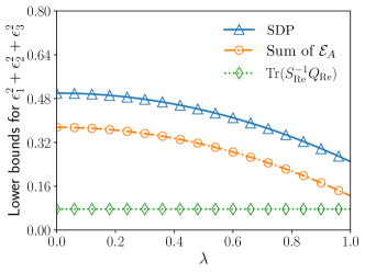
Figure 2: Lower bounds for the errors of the simultaneous measurement of $(X_{1},X_{2},X_{3})$ given by (i) bound that obtained from $\mathrm{Tr}(S_{\text{Re}}^{-1}Q_{\text{Re}})$; (ii) the simple summation of the analytical bound $\mathcal{E}_{A}$ for all pairs and (iii) $\mathcal{E}_{0}$ that can be computed with SDP.

I.2 Example: Tradeoff relation for the estimation of multiple parameters in a qubit

Bounds obtained from $\mathrm{Tr}(S_{\text{Re}}^{-1}Q_{\text{Re}})$:

The error-tradeoff relation for multiple observables can be used to obtain tradeoff relation in multiparameter quantum estimation. Here we consider the simultaneous estimation of the three parameters $(\lambda,\theta,\varphi)$ in $\rho=\frac{1}{2}(I+r_{x}\sigma_{x}+r_{y}\sigma_{y}+r_{z}\sigma_{z})$, where $r_{x}=\lambda\sin\theta\cos\varphi$, $r_{y}=\lambda\sin\theta\sin\varphi$, and $r_{z}=\lambda\cos\theta$, here $|\lambda|\leq 1$.

For any measurement on $\rho$, the classical Fisher information matrix, $F_{C}$, is bounded as in Eq.(140) with

$$\mathrm{Tr}[F_{Q}^{-1}F_{C}]\leq 3-\left(\sqrt{\|F_{Q}^{-\frac{1}{2}}\tilde{S}_{\text{Im}}F_{Q}^{-\frac{1}{2}}\|_{F}+1}-1\right)^{2},$$ (165)

The SLDs for $(\lambda,\theta,\varphi)$ are given by

$$L_{\lambda}=\frac{1}{1-\lambda^{2}}(\vec{n}\cdot\vec{\sigma}-\lambda I),\quad L_{\theta}=\lambda(\partial_{\theta}\vec{n}\cdot\vec{\sigma}),\quad L_{\varphi}=\lambda(\partial_{\varphi}\vec{n}\cdot\vec{\sigma}),$$ (166)

here $\vec{n}=(\sin\theta\cos\varphi,\sin\theta\sin\varphi,\cos\theta)$, $\vec{\sigma}=(\sigma_{x},\sigma_{y},\sigma_{z})$, and the quantum Fisher information matrix is

$$F_{Q}=\begin{pmatrix}\frac{1}{1-\lambda^{2}}&0&0\\ 0&\lambda^{2}&0\\ 0&0&\lambda^{2}\sin^{2}\theta\end{pmatrix}.$$ (167)

We can use Eq.(145) to maximize $\tilde{S}_{\text{Im}}$ over $\{|u_{q}\rangle\}$. Note that under the reparameterization which makes $F_{Q}=I$, we have $F_{Q}^{-\frac{1}{2}}\tilde{S}_{\text{Im}}F_{Q}^{-\frac{1}{2}}=\tilde{S}_{\text{Im}}$. The SLD operators under this reparametrization are given by $\tilde{L}_{k}=\sum_{j}(F_{Q}^{-\frac{1}{2}})_{jk}L_{j}$, i.e.,

$$\tilde{L}_{\lambda}=\frac{1}{\sqrt{1-\lambda^{2}}}(\vec{n}\cdot\vec{\sigma}-\lambda I),\quad\tilde{L}_{\theta}=\partial_{\theta}\vec{n}\cdot\vec{\sigma},\quad\tilde{L}_{\varphi}=\frac{1}{|\sin\theta|}(\partial_{\varphi}\vec{n}\cdot\vec{\sigma}).$$ (168)

From Eq.(157) we can obtain $\sqrt{\rho}=\frac{1}{2}(pI+q\vec{n}\cdot{\sigma})$, thus we have

$$\mathcal{X}_{12}=\frac{1}{2i}\sqrt{\rho}[\tilde{L}_{\lambda},\tilde{L}_{\theta}]\sqrt{\rho} =\frac{1}{2\sin\theta}(\partial_{\varphi}\vec{n}\cdot\vec{\sigma}),$$ (169)

$$\mathcal{X}_{23}=\frac{1}{2i}\sqrt{\rho}[\tilde{L}_{\theta},\tilde{L}_{\varphi}]\sqrt{\rho} =\frac{|\sin\theta|}{2\sin\theta}\left(\lambda I+\vec{n}\cdot\vec{\sigma}\right),$$

$$\mathcal{X}_{31}=\frac{1}{2i}\sqrt{\rho}[\tilde{L}_{\varphi},\tilde{L}_{\lambda}]\sqrt{\rho} =\frac{|\sin\theta|}{2\sin\theta}\left(\partial_{\theta}\vec{n}\cdot\vec{\sigma}\right),$$

which gives

$$x_{12}=-x_{21}=\frac{1}{\sin\theta}\partial_{\varphi}\vec{n},\quad x_{23}=-x_{32}=\frac{|\sin\theta|}{\sin\theta}\vec{n},\quad x_{13}=-x_{31}=-\frac{|\sin\theta|}{\sin\theta}\partial_{\theta}\vec{n}.$$ (170)

Note that $x_{11}=x_{22}=x_{33}=\mathbf{0}$, it is then easy to obtain $S^{xx}=\sum_{j,k=1}^{3}x_{jk}x_{jk}^{T}=2I$. In this case $\{|u_{q}\rangle\}$ can be chosen arbitrarily and we always have $\lambda_{\max}(S^{xx})=2$. It is also straightforward to obtain $\sum_{jk}|w_{jk}|^{2}=\sum_{jk}|\mathrm{Tr}(\mathcal{X}_{jk})|^{2}=2\lambda^{2}\leq 2$, thus

$$\max_{\{|u_{q}\rangle\}}\|F_{Q}^{-\frac{1}{2}}\tilde{S}_{\text{Im}}F_{Q}^{-\frac{1}{2}}\|_{F}=\sqrt{2}.$$ (171)

This leads to a tradeoff relation for the estimation of $\{\lambda,\theta,\varphi\}$ as

$$\mathrm{Tr}[F_{Q}^{-1}F_{C}]\leq 3-\left(\sqrt{\max_{\{|u_{q}\rangle\}}\|F_{Q}^{-\frac{1}{2}}\tilde{S}_{\text{Im}}F_{Q}^{-\frac{1}{2}}\|_{F}+1}-1\right)^{2}=3-\left(\sqrt{\sqrt{2}+1}-1\right)^{2}.$$ (172)

Bounds obtained from $\mathcal{E}_{A}$ and the SDP $\mathcal{E}_{0}$:

By doing summation over the analytical bound $\mathcal{E}_{A}$ for each pairs of $(\tilde{L}_{j},\tilde{L}_{k})$, we directly have

$$\mathrm{Tr}[F_{Q}^{-1}F_{C}]\leq n-\frac{1}{2(n-1)}\|C\|_{F}^{2},$$ (173)

with the $jk$-th entry of $C$ given as $(C)_{jk}=\sqrt{\mathcal{E}_{A}(\tilde{L}_{j},\tilde{L}_{k})}$. Again for the ease of comparison, we choose specific values of $\theta=\frac{\pi}{2}$, $\phi=0$. Substituting $\tilde{L}_{\lambda}$, $\tilde{L}_{\theta}$, $\tilde{L}_{\varphi}$ in $\mathcal{E}_{A}(\tilde{L}_{j},\tilde{L}_{k})$, we directly have $\mathcal{E}_{A}(\tilde{L}_{\lambda},\tilde{L}_{\theta})=\mathcal{E}_{A}(\tilde{L}_{\theta},\tilde{L}_{\varphi})=\mathcal{E}_{A}(\tilde{L}_{\varphi},\tilde{L}_{\lambda})=1$, and

$$\mathrm{Tr}[F_{Q}^{-1}F_{C}]\leq 3-\frac{1}{4}\|C\|_{F}^{2}=\frac{3}{2}.$$ (174)

By substituting $\tilde{L}_{\lambda}$, $\tilde{L}_{\theta}$, $\tilde{L}_{\varphi}$, the SDP $\mathcal{E}_{0}$ also gives a bound directly as $\mathrm{Tr}[F_{Q}^{-1}F_{C}]\leq n-\mathcal{E}_{0}=1$, which is the tightest among all bounds and coincides with the Gill-Massar bound for qubit states.

I.3 Example: Tradeoff relation under collective measurement

While the tradeoff relation is obtained under local measurements, it can also be used to obtain tradeoff relations for collective measurements on $p$ copies of the states by simply replacing $\rho$ with $\rho_{x}^{\otimes p}$.

As an example we consider the simultaneous estimation of the three parameters $(\lambda,\theta,\varphi)$ in a state $\rho=\frac{1}{2}(I+r_{x}\sigma_{x}+r_{y}\sigma_{y}+r_{z}\sigma_{z})$, where $r_{x}=\lambda\sin\theta\cos\varphi$, $r_{y}=\lambda\sin\theta\sin\varphi$, and $r_{z}=\lambda\cos\theta$, $|\lambda|\leq 1$. But different from previous section, here we also allow collective measurement on two-copies of the state, $\rho\otimes\rho$.

To obtain the tradeoff relation under the collective measurement on 2-copies of the state, we can simply treat $\rho\otimes\rho$ as a larger single state. Its SLDs are given by $L_{j2}=L_{j}\otimes I+I\otimes L_{j}$ with $j=\lambda,\theta,\varphi$ and the quantum Fisher information matrix is $F_{Q2}=2F_{Q}$ with $F_{Q}$ as the quantum Fisher information matrix of a single $\rho$.

Bounds obtained from $\mathrm{Tr}(S_{\text{Re}}^{-1}Q_{\text{Re}})$:

If we choose $\{|u_{q}\rangle\}$ as the computational basis with $|u_{0}\rangle=|00\rangle$, $|u_{1}\rangle=|01\rangle$, $|u_{2}\rangle=|10\rangle$, $|u_{3}\rangle=|11\rangle$, the corresponding $S_{u_{q},\text{Im}2}$ are given by

$$S_{u_{0},\text{Im}2} =\begin{pmatrix}0&0&-\frac{\lambda(1+\lambda\cos\theta)\sin^{2}\theta}{2\sqrt{1-\lambda^{2}}}\\ 0&0&-\frac{1}{2}\lambda^{2}\sin\theta(1+\lambda\cos\theta)(\cos\theta+\lambda)\\ \frac{\lambda(1+\lambda\cos\theta)\sin^{2}\theta}{2\sqrt{1-\lambda^{2}}}&\frac{1}{2}\lambda^{2}\sin\theta(1+\lambda\cos\theta)(\cos\theta+\lambda)&0\end{pmatrix}$$ (175)

$$S_{u_{1},\text{Im}2} =S_{u_{2},\text{Im}2}=\begin{pmatrix}0&0&\frac{\lambda^{2}\cos\theta\sin^{2}\theta}{2\sqrt{1-\lambda^{2}}}\\ 0&0&-\frac{1}{2}\lambda^{3}\sin^{3}\theta\\ -\frac{\lambda^{2}\cos\theta\sin^{2}\theta}{2\sqrt{1-\lambda^{2}}}&\frac{1}{2}\lambda^{3}\sin^{3}\theta&0\end{pmatrix}$$

$$S_{u_{3},\text{Im}2} =\begin{pmatrix}0&0&\frac{\lambda(1-\lambda\cos\theta)\sin^{2}\theta}{2\sqrt{1-\lambda^{2}}}\\ 0&0&\frac{1}{2}\lambda^{2}\sin\theta(1-\lambda\cos\theta)(\cos\theta-\lambda)\\ -\frac{\lambda(1-\lambda\cos\theta)\sin^{2}\theta}{2\sqrt{1-\lambda^{2}}}&-\frac{1}{2}\lambda^{2}\sin\theta(1-\lambda\cos\theta)(\cos\theta-\lambda)&0\end{pmatrix}$$

The optimal $\|F_{Q2}^{-\frac{1}{2}}\tilde{S}_{\text{Im}2}F_{Q2}^{-\frac{1}{2}}\|_{F}$ is thus given by the maximum of the following values,

$$\|F_{Q2}^{-\frac{1}{2}}(S_{u_{0},\text{Im}2}+S_{u_{1},\text{Im}2}+S_{u_{2},\text{Im}2}+S_{u_{3},\text{Im}2})F_{Q2}^{-\frac{1}{2}}\|_{F} =\sqrt{2}|\lambda|,$$ (176)

$$\|F_{Q2}^{-\frac{1}{2}}(S_{u_{0},\text{Im}2}+S_{u_{1},\text{Im}2}^{T}+S_{u_{2},\text{Im}2}^{T}+S_{u_{3},\text{Im}2})F_{Q2}^{-\frac{1}{2}}\|_{F} =\sqrt{2}|\lambda\cos\theta|,$$

$$\|F_{Q2}^{-\frac{1}{2}}(S_{u_{0},\text{Im}2}+S_{u_{1},\text{Im}2}+S_{u_{2},\text{Im}2}+S_{u_{3},\text{Im}2}^{T})F_{Q2}^{-\frac{1}{2}}\|_{F} =\sqrt{\frac{1}{2}(1+\lambda^{2})(1+\lambda^{2}\cos^{2}\theta)+\lambda^{3}\cos\theta\sin^{2}\theta},$$

$$\|F_{Q2}^{-\frac{1}{2}}(S_{u_{0},\text{Im}2}+S_{u_{1},\text{Im}2}^{T}+S_{u_{2},\text{Im}2}^{T}+S_{u_{3},\text{Im}2}^{T})F_{Q2}^{-\frac{1}{2}}\|_{F} =\sqrt{\frac{1}{2}(1+\lambda^{2})(1+\lambda^{2}\cos^{2}\theta)-\lambda^{3}\cos\theta\sin^{2}\theta}.$$

By simply replacing $F_{Q}$ and $\tilde{S}_{\text{Im}}$ with $F_{Q2}$ and $\tilde{S}_{\text{Im}2}$ in Eq.(140), we can get

$$\frac{1}{2}\mathrm{Tr}[F_{Q}^{-1}F_{C2}] \leq 3-(\sqrt{\|F_{Q2}^{-\frac{1}{2}}\tilde{S}_{\text{Im}2}F_{Q2}^{-\frac{1}{2}}\|_{F}+1}-1)^{2}$$ (177)

$$=3-\left(\sqrt{\max\left\{\sqrt{2}|\lambda|,\sqrt{\frac{1}{2}(1+\lambda^{2})(1+\lambda^{2}\cos^{2}\theta)+|\lambda^{3}\cos\theta\sin^{2}\theta|}\right\}+1}-1\right)^{2},$$

here $F_{C2}$ denotes the classical Fisher information matrix under the collective measurement on $\rho\otimes\rho$, $\frac{1}{2}F_{C2}$ can be regarded as the average Fisher information on each $\rho$. This bounds the achievable precision limit under the collective measurements on 2 copies of the quantum state. Specifically for $\theta=\frac{\pi}{2}$, we have

$$\frac{1}{2}\mathrm{Tr}[F_{Q}^{-1}F_{C2}]\leq 3-\left(\sqrt{\max\left\{\sqrt{2}|\lambda|,\sqrt{\frac{1}{2}(1+\lambda^{2})}\right\}+1}-1\right)^{2}.$$ (178)

Bounds obtained from $\mathcal{E}_{A}$ and the SDP $\mathcal{E}_{0}$:

Under the reparameterization that $F_{Q2}=2F_{Q}=I$, by replacing $(X_{j},X_{k})$ with $(\tilde{L}_{j2},\tilde{L}_{k2})$, the bound $\mathcal{E}_{A}$ gives

$$\epsilon_{j}^{2}+\epsilon_{k}^{2}=1-(F_{C2})_{jj}+1-(F_{C2})_{kk}\geq\mathcal{E}_{A}(\tilde{L}_{j2},\tilde{L}_{k2}).$$ (179)

By doing summations over each pairs of $(j,k)$, we directly have

$$\frac{1}{2}\mathrm{Tr}[F_{Q}^{-1}F_{C2}]\leq n-\frac{1}{2(n-1)}\|C_{2}\|_{F}^{2},$$ (180)

with the $jk$-th entry of $C_{2}$ given as $(C_{2})_{jk}=\sqrt{\mathcal{E}_{A}(\tilde{L}_{j2},\tilde{L}_{k2})}$. Again for the ease of comparison, we choose specific values of $\theta=\frac{\pi}{2}$, $\phi=0$. Substituting $\tilde{L}_{\lambda 2}$, $\tilde{L}_{\theta 2}$, $\tilde{L}_{\varphi 2}$ in $\mathcal{E}_{A}(\tilde{L}_{j2},\tilde{L}_{k2})$, we can directly obtain a bound. By substituting $\tilde{L}_{\lambda 2}$, $\tilde{L}_{\theta 2}$, $\tilde{L}_{\varphi 2}$, the SDP $\mathcal{E}_{0}$ also gives a bound directly as $\frac{1}{2}\mathrm{Tr}[F_{Q}^{-1}F_{C2}]\leq n-\mathcal{E}_{0}$. Fig. 3 then illustrate the comparison among the three bounds with $\lambda$ varies from 0 to 1.

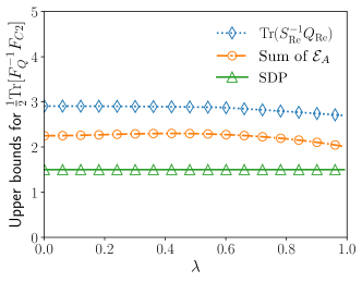
Figure 3: Upper bounds for $\frac{1}{2}\mathrm{Tr}[F_{Q}^{-1}F_{C2}]$ given by (i) bound that obtained from $\mathrm{Tr}(S_{\text{Re}}^{-1}Q_{\text{Re}})$; (ii) the simple summation of the analytical bound $\mathcal{E}_{A}$ for all pairs and (iii) $\mathcal{E}_{0}$ that can be computed with SDP.

I.4 Example: Tradeoff relation for the estimation of multiple parameters in three qubits

We provide an example with three qubits to show that the analytical bound obtained from $\mathrm{Tr}(S_{\text{Re}}^{-1}Q_{\text{Re}})$ can be tighter than the simple summation over the bounds $\mathcal{E}_{A}$ for each pairs of observables.

We consider a parameterized pure state $|\psi\rangle=\sin\theta_{0}|\psi_{1}\rangle+\cos\theta_{0}e^{i\phi_{0}}|\psi_{2}\rangle$, where

$$|\psi_{1}\rangle=\sin\theta_{1}\sin\theta_{2}|001\rangle+\sin\theta_{1}\cos\theta_{2}e^{i\phi_{1}}|010\rangle+\cos\theta_{1}e^{i\phi_{2}}|100\rangle,$$ (181)

$$|\psi_{2}\rangle=\sin\theta_{3}\sin\theta_{4}|110\rangle+\sin\theta_{3}\cos\theta_{4}e^{i\phi_{3}}|101\rangle+\cos\theta_{3}e^{i\phi_{4}}|011\rangle.$$

We first consider the estimation of $\{\theta_{0},\theta_{1},\theta_{2},\phi_{1},\phi_{2}\}$ in $|\psi\rangle=\sin\theta_{0}|\psi_{1}\rangle+\cos\theta_{0}e^{i\phi_{0}}|\psi_{2}\rangle$. In this case $F_{Q}=\begin{pmatrix}F_{Q1}&\mathbf{0}\\ \mathbf{0}&F_{Q2}\end{pmatrix}$ with

$$F_{Q1} =\operatorname{diag}\{4,4\sin^{2}\theta_{0},4\sin^{2}\theta_{0}\sin^{2}\theta_{1}\},$$ (182)

$$F_{Q2} =\begin{pmatrix}4\sin^{2}\theta_{0}\sin^{2}\theta_{1}\cos^{2}\theta_{2}(1-\sin^{2}\theta_{0}\sin^{2}\theta_{1}\cos^{2}\theta_{2})&-\sin^{4}\theta_{0}\sin^{2}2\theta_{1}\cos^{2}\theta_{2}\\ -\sin^{4}\theta_{0}\sin^{2}2\theta_{1}\cos^{2}\theta_{2}&4\sin^{2}\theta_{0}\cos^{2}\theta_{1}(1-\sin^{2}\theta_{0}\cos^{2}\theta_{1})\end{pmatrix},$$

and $S_{\text{Im}}=\begin{pmatrix}\mathbf{0}&S_{\text{Im}1}^{\dagger}\\ S_{\text{Im}1}&\mathbf{0}\end{pmatrix}$ where

$$S_{\text{Im}1}=2\begin{pmatrix}\sin 2\theta_{0}\sin^{2}\theta_{1}\cos^{2}\theta_{2}&\sin^{2}\theta_{0}\sin 2\theta_{1}\cos^{2}\theta_{2}&-\sin^{2}\theta_{0}\sin^{2}\theta_{1}\sin 2\theta_{2}\\ \sin 2\theta_{0}\cos^{2}\theta_{1}&-\sin^{2}\theta_{0}\sin 2\theta_{1}&0\end{pmatrix}.$$ (183)

Thus

$$F_{Q}^{-\frac{1}{2}}S_{\text{Im}}F_{Q}^{-\frac{1}{2}}=\begin{pmatrix}F_{Q1}^{-\frac{1}{2}}&\mathbf{0}\\ \mathbf{0}&F_{Q2}^{-\frac{1}{2}}\end{pmatrix}\begin{pmatrix}\mathbf{0}&S_{\text{Im}1}^{\dagger}\\ S_{\text{Im}1}&\mathbf{0}\end{pmatrix}\begin{pmatrix}F_{Q1}^{-\frac{1}{2}}&\mathbf{0}\\ \mathbf{0}&F_{Q2}^{-\frac{1}{2}}\end{pmatrix}=\begin{pmatrix}\mathbf{0}&F_{Q1}^{-\frac{1}{2}}S_{\text{Im}1}^{\dagger}F_{Q2}^{-\frac{1}{2}}\\ F_{Q2}^{-\frac{1}{2}}S_{\text{Im}1}F_{Q1}^{-\frac{1}{2}}&\mathbf{0}\end{pmatrix},$$ (184)

and

$$\|F_{Q}^{-\frac{1}{2}}S_{\text{Im}}F_{Q}^{-\frac{1}{2}}\|_{F}^{2}=2\|F_{Q2}^{-\frac{1}{2}}S_{\text{Im}1}F_{Q1}^{-\frac{1}{2}}\|_{F}^{2}=2\mathrm{Tr}\left(F_{Q2}^{-1}S_{\text{Im}1}F_{Q1}^{-1}S_{\text{Im}1}^{\dagger}\right)=4.$$ (185)

We then have

$$\mathrm{Tr}[F_{Q}^{-1}F_{C}]\leq n-\left(\sqrt{\|F_{Q}^{-\frac{1}{2}}\tilde{S}_{\text{Im}}F_{Q}^{-\frac{1}{2}}\|_{F}+1}-1\right)^{2}=5-(\sqrt{3}-1)^{2}\approx 4.464.$$ (186)

Compared with the simple summation of the analytical bound for pairs of the observables, which cannot be tighter than $n-\frac{1}{2(n-1)}\|F_{Q}^{-\frac{1}{2}}S_{\text{Im}}F_{Q}^{-\frac{1}{2}}\|_{F}^{2}=5-\frac{1}{8}\times 4=\frac{9}{2}$, the bound obtained from $\mathrm{Tr}(S_{\text{Re}}^{-1}Q_{\text{Re}})$ is strictly tighter. The tight bound can be obtained by computing the SDP $\mathcal{E}_{0}$. Specifically, for $\theta_{j}=\pi/4$, $1\leq j\leq 4$ and $\phi_{k}=\pi/4$, $0\leq k\leq 4$, we compare the three bounds with $\theta_{0}$ varies from $0$ to $\pi/2$. As illustrated in Fig. 4(a), the analytical bound obtained from $\mathrm{Tr}(S_{\text{Re}}^{-1}Q_{\text{Re}})$ is tighter than the simple summation of $\mathcal{E}_{A}$ for all pairs, while the tight bound is given by $\mathcal{E}_{0}$ that can be computed with SDP, which is approximately $\mathrm{Tr}[F_{Q}^{-1}F_{C}]\leq 3$.

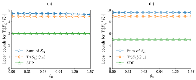
Figure 4: Upper bounds for $\mathrm{Tr}[F_{Q}^{-1}F_{C}]$ of (a) estimation of $n=5$ parameters $\{\theta_{0},\theta_{1},\theta_{2},\phi_{1},\phi_{2}\}$, (b) estimation of $n=10$ parameters $\{\theta_{0},\theta_{1},\theta_{2},\theta_{3},\theta_{4},\phi_{0},\phi_{1},\phi_{2},\phi_{3},\phi_{4}\}$. Here the bounds are given by (i) bound that obtained from $\mathrm{Tr}(S_{\text{Re}}^{-1}Q_{\text{Re}})$; (ii) the simple summation of the analytical bound $\mathcal{E}_{A}$ for all pairs and (iii) $\mathcal{E}_{0}$ that can be computed with SDP.

For the estimation of the full set, $\{\theta_{0},\theta_{1},\theta_{2},\theta_{3},\theta_{4},\phi_{0},\phi_{1},\phi_{2},\phi_{3},\phi_{4}\}$, we can obtain the bound numerically. Specifically, for $\theta_{j}=\pi/4$ and $\phi_{k}=\pi/4$, $0\leq j,k\leq 4$, we have $F_{Q}=\begin{pmatrix}F_{Q1}&\mathbf{0}\\ \mathbf{0}&F_{Q2}\end{pmatrix}$ where

$$F_{Q1}=\operatorname{diag}\{4,2,1,2,1\},F_{Q2}=\begin{pmatrix}1&-\frac{1}{4}&-\frac{1}{2}&\frac{1}{4}&\frac{1}{2}\\ -\frac{1}{4}&\frac{7}{16}&-\frac{1}{8}&-\frac{1}{16}&-\frac{1}{8}\\ -\frac{1}{2}&-\frac{1}{8}&\frac{3}{4}&-\frac{1}{8}&-\frac{1}{4}\\ \frac{1}{4}&-\frac{1}{16}&-\frac{1}{8}&\frac{7}{16}&-\frac{1}{8}\\ \frac{1}{2}&-\frac{1}{8}&-\frac{1}{4}&-\frac{1}{8}&\frac{3}{4}\end{pmatrix},$$ (187)

and $S_{\text{Im}}=\begin{pmatrix}\mathbf{0}&S_{\text{Im}1}^{\dagger}\\ S_{\text{Im}1}&\mathbf{0}\end{pmatrix}$ with

$$S_{\text{Im}1}=\begin{pmatrix}-2&0&0&0&0\\ \frac{1}{2}&\frac{1}{2}&-\frac{1}{2}&0&0\\ 1&-1&0&0&0\\ -\frac{1}{2}&0&0&\frac{1}{2}&-\frac{1}{2}\\ -1&0&0&-1&0\end{pmatrix}.$$ (188)

We then have

$$\|F_{Q}^{-\frac{1}{2}}S_{\text{Im}}F_{Q}^{-\frac{1}{2}}\|_{F}^{2}=2\|F_{Q2}^{-\frac{1}{2}}S_{\text{Im}1}F_{Q1}^{-\frac{1}{2}}\|_{F}^{2}=2\mathrm{Tr}\left(F_{Q2}^{-1}S_{\text{Im}1}F_{Q1}^{-1}S_{\text{Im}1}^{\dagger}\right)=10,$$ (189)

and

$$\mathrm{Tr}[F_{Q}^{-1}F_{C}]\leq n-\left(\sqrt{\|F_{Q}^{-\frac{1}{2}}\tilde{S}_{\text{Im}}F_{Q}^{-\frac{1}{2}}\|_{F}+1}-1\right)^{2}=10-\left(\sqrt{\sqrt{10}+1}-1\right)^{2}\approx 8.918.$$ (190)

Compared with the simple summation of the analytical bound for pairs of the observables, which cannot be tighter than $n-\frac{1}{2(n-1)}\|F_{Q}^{-\frac{1}{2}}S_{\text{Im}}F_{Q}^{-\frac{1}{2}}\|_{F}^{2}=10-\frac{1}{18}\times 10=\frac{85}{9}\approx 9.444$, the bound obtained from $\mathrm{Tr}(S_{\text{Re}}^{-1}Q_{\text{Re}})$ is strictly tighter. The tight bound can be obtained by computing the SDP $\mathcal{E}_{0}$. For $\theta_{j}=\pi/4$, $1\leq j\leq 4$ and $\phi_{k}=\pi/4$, $0\leq k\leq 4$, we compare the three bounds with $\theta_{0}$ varies from $0$ to $\pi/2$. As illustrated in Fig. 4(b), the analytical bound obtained from $\mathrm{Tr}(S_{\text{Re}}^{-1}Q_{\text{Re}})$ is tighter than the simple summation of $\mathcal{E}_{A}$ for all pairs, while the tight bound is given by $\mathcal{E}_{0}$ that can be computed with SDP, which is approximately $\mathrm{Tr}[F_{Q}^{-1}F_{C}]\leq 5$.

References

- [1] W. Heisenberg. úber den anschaulichen inhalt der quantentheoretischen kinematik und mechanik. Z. Phys., 43:172, 1927.
- [2] H. P. Robertson. The uncertainty principle. Phys. Rev., 34:163–164, 1929.
- [3] E. Schrodinger. About Heisenberg uncertainty relation. Sitzungsber. Preuss. Akad. Wiss. Berlin (Math. Phys. ), 19:296–303, 1930.
- [4] H. P. Robertson. An indeterminacy relation for several observables and its classical interpretation. Phys. Rev., 46:794–801, Nov 1934.
- [5] E. Arthurs and J. L. Kelly Jr. On the simultaneous measurement of a pair of conjugate observables. Bell System Technical Journal, 44(4):725–729, 1965.
- [6] E. Arthurs and M. S. Goodman. Quantum correlations: A generalized heisenberg uncertainty relation. Phys. Rev. Lett., 60:2447–2449, Jun 1988.
- [7] Masanao Ozawa. Universally valid reformulation of the heisenberg uncertainty principle on noise and disturbance in measurement. Phys. Rev. A, 67:042105, Apr 2003.
- [8] Masanao Ozawa. Uncertainty relations for joint measurements of noncommuting observables. Physics Letters A, 320(5):367–374, 2004.
- [9] Masanao Ozawa. Uncertainty relations for noise and disturbance in generalized quantum measurements. Annals of Physics, 311(2):350–416, 2004.
- [10] Masanao Ozawa. Physical content of heisenberg’s uncertainty relation: limitation and reformulation. Physics Letters A, 318(1):21–29, 2003.
- [11] Masanao Ozawa. Heisenberg’s uncertainty relation: Violation and reformulation. Journal of Physics: Conference Series, 504(1):012024, apr 2014.
- [12] Michael J. W. Hall. Prior information: How to circumvent the standard joint-measurement uncertainty relation. Phys. Rev. A, 69:052113, May 2004.
- [13] Cyril Branciard. Error-tradeoff and error-disturbance relations for incompatible quantum measurements. Proceedings of the National Academy of Sciences of the United States of America, 110:6742, 2013.
- [14] Cyril Branciard. Deriving tight error-trade-off relations for approximate joint measurements of incompatible quantum observables. Phys. Rev. A, 89:022124, Feb 2014.
- [15] Xiao-Ming Lu, Sixia Yu, Kazuo Fujikawa, and C. H. Oh. Improved error-tradeoff and error-disturbance relations in terms of measurement error components. Phys. Rev. A, 90:042113, Oct 2014.
- [16] M. Ozawa. Error-disturbance relations in mixed states. Eprint Arxiv, arXiv:1404.3388, 2014.
- [17] Francesco Buscemi, Michael J. W. Hall, Masanao Ozawa, and Mark M. Wilde. Noise and disturbance in quantum measurements: An information-theoretic approach. Phys. Rev. Lett., 112:050401, Feb 2014.
- [18] Paul Busch, Pekka Lahti, and Reinhard F. Werner. Colloquium: Quantum root-mean-square error and measurement uncertainty relations. Rev. Mod. Phys., 86:1261–1281, Dec 2014.
- [19] Paul Busch, Teiko Heinonen, and Pekka Lahti. Heisenberg’s uncertainty principle. Physics Reports, 452(6):155–176, 2007.
- [20] Hui-Hui Qin, Ting-Gui Zhang, Leonardo Jost, Chang-Pu Sun, Xianqing Li-Jost, and Shao-Ming Fei. Uncertainties of genuinely incompatible triple measurements based on statistical distance. Phys. Rev. A, 99:032107, Mar 2019.
- [21] Paul Busch, Pekka Lahti, and Reinhard F. Werner. Proof of heisenberg’s error-disturbance relation. Phys. Rev. Lett., 111:160405, Oct 2013.
- [22] Wenchao Ma, Zhihao Ma, Hengyan Wang, Zhihua Chen, Ying Liu, Fei Kong, Zhaokai Li, Xinhua Peng, Mingjun Shi, Fazhan Shi, Shao-Ming Fei, and Jiangfeng Du. Experimental test of heisenberg’s measurement uncertainty relation based on statistical distances. Phys. Rev. Lett., 116:160405, Apr 2016.
- [23] Ya-Li Mao, Hu Chen, Chang Niu, Zheng-Da Li, Sixia Yu, and Jingyun Fan. Testing Heisenberg’s measurement uncertainty relation of three observables. arXiv, 2211.09389, Nov 2022.
- [24] Michael A Taylor and Warwick P Bowen. Quantum metrology and its application in biology. Physics Reports, 615:1–59, 2016.
- [25] Ryszard Horodecki, Paweł Horodecki, Michał Horodecki, and Karol Horodecki. Quantum entanglement. Rev. Mod. Phys., 81:865–942, Jun 2009.
- [26] M A Nielsen and I L Chuang. Quantum Computation and Quantum Information. Cambridge University Press, Cambridge, UK, 2000.
- [27] Jing Yang, Shengshi Pang, Yiyu Zhou, and Andrew N. Jordan. Optimal measurements for quantum multiparameter estimation with general states. Phys. Rev. A, 100:032104, Sep 2019.
- [28] Hongzhen Chen, Yu Chen, and Haidong Yuan. Information geometry under hierarchical quantum measurement. Phys. Rev. Lett., 128:250502, Jun 2022.
- [29] Hongzhen Chen, Yu Chen, and Haidong Yuan. Incompatibility measures in multiparameter quantum estimation under hierarchical quantum measurements. Phys. Rev. A, 105:062442, Jun 2022.
- [30] Harald Cramér. Mathematical Methods of Statistics. Princeton University Press, Princeton, NJ, 1946.
- [31] R. A. Fisher. On the mathematical foundations of theoretical statistics. Philos. Trans. R. Soc. Lond. A, 222:309–368, 1922.
- [32] Carl W. Helstrom. Quantum Detection and Estimation Theory. Academic Press, New York, 1976.
- [33] A. S. Holevo. Probabilistic and Statistical Aspects of Quantum Theory. North-Holland, Amsterdam, 1982.
- [34] Keiji Matsumoto. A geometrical approach to quantum estimation theory. arXiv, 2111.09667, November 2021.
- [35] Richard D. Gill and Serge Massar. State estimation for large ensembles. Phys. Rev. A, 61:042312, Mar 2000.
- [36] Masahito Hayashi and Keiji Matsumoto. Statistical model with measurement degree of freedom and quantum physics. In Masahito Hayashi, editor, Asymptotic theory of quantum statistical inference: Selected Papers, Singapore, 2005. World scientific. Original Japanese version was published in Surikaiseki Kenkyusho Kokyuroku, 1055:96-110, 1998.
- [37] Huangjun Zhu and Masahito Hayashi. Universally fisher-symmetric informationally complete measurements. Phys. Rev. Lett., 120:030404, Jan 2018.
- [38] Xiao-Ming Lu and Xiaoguang Wang. Incorporating heisenberg’s uncertainty principle into quantum multiparameter estimation. Phys. Rev. Lett., 126:120503, Mar 2021.
- [39] Jun Suzuki. Explicit formula for the holevo bound for two-parameter qubit-state estimation problem. Journal of Mathematical Physics, 57(4):042201, 2016.
- [40] Jasminder S. Sidhu, Yingkai Ouyang, Earl T. Campbell, and Pieter Kok. Tight bounds on the simultaneous estimation of incompatible parameters. Phys. Rev. X, 11:011028, Feb 2021.
- [41] H. Nagaoka. A new approach to cramer–rao bounds for quantum state estimation. In Masahito Hayashi, editor, Asymptotic theory of quantum statistical inference: Selected Papers, Singapore, 2005. World scientific. Originally published as IEICE Technical Report, 89, 228, IT 89–42, 9–14 (1989).
- [42] H. Nagaoka. A generalization of the simultaneous diagonalization of hermitian matrices and its relation to quantum estimation theory. In Masahito Hayashi, editor, Asymptotic theory of quantum statistical inference: Selected Papers, Singapore, 2005. World scientific.
- [43] Lorcán O. Conlon, Jun. Suzuki, Ping Koy Lam, and Syed M. Assad. Efficient computation of the nagaoka–hayashi bound for multiparameter estimation with separable measurements. npj Quantum Information, 7:110, Jul 2021.
- [44] F. Albarelli, M. Barbieri, M.G. Genoni, and I. Gianani. A perspective on multiparameter quantum metrology: From theoretical tools to applications in quantum imaging. Physics Letters A, 384(12):126311, 2020.
- [45] Federico Belliardo and Vittorio Giovannetti. Incompatibility in quantum parameter estimation. New Journal of Physics, 23(6):063055, jun 2021.
- [46] Angelo Carollo, Bernardo Spagnolo, Alexander A Dubkov, and Davide Valenti. On quantumness in multi-parameter quantum estimation. Journal of Statistical Mechanics: Theory and Experiment, 2019(9):094010, sep 2019.
- [47] Sammy Ragy, Marcin Jarzyna, and Rafal Demkowicz-Dobrzański. Compatibility in multiparameter quantum metrology. Phys. Rev. A, 94:052108, Nov 2016.
- [48] Yu Chen and Haidong Yuan. Maximal quantum fisher information matrix. New Journal of Physics, 19(6):063023, jun 2017.
- [49] Jing Liu, Haidong Yuan, Xiao-Ming Lu, and Xiaoguang Wang. Quantum fisher information matrix and multiparameter estimation. Journal of Physics A: Mathematical and Theoretical, 53(2):023001, dec 2020.
- [50] Hongzhen Chen and Haidong Yuan. Optimal joint estimation of multiple rabi frequencies. Phys. Rev. A, 99:032122, Mar 2019.
- [51] R. Demkowicz-Dobrzański, W. Górecki, and M. Guţă. Multi-parameter estimation beyond quantum fisher information. J. Phys. A: Math. Theor., 53:363001, 2020.
- [52] Jasminder S. Sidhu and Pieter Kok. Geometric perspective on quantum parameter estimation. AVS Quantum Sci., 2:014701, 2020.
- [53] M. D. Vidrighin, G. Donati, M. G. Genoni, X.-M. Jin, W. S. Kolthammer, M. S. Kim, A. Datta, M. Barbieri, and I. A. Walmsley. Joint estimation of phase and phase diffusion for quantum metrology. Nat. Commun., 5:3532, 2014.
- [54] Philip J. D. Crowley, Animesh Datta, Marco Barbieri, and I. A. Walmsley. Tradeoff in simultaneous quantum-limited phase and loss estimation in interferometry. Phys. Rev. A, 89:023845, Feb 2014.
- [55] J.-D. Yue, Y.-R. Zhang, and H Fan. Quantum-enhanced metrology for multiple phase estimation with noise. Sci. Rep., 4:5933, 2014.
- [56] Yu-Ran Zhang and Heng Fan. Quantum metrological bounds for vector parameters. Phys. Rev. A, 90:043818, Oct 2014.
- [57] Jing Liu and Haidong Yuan. Control-enhanced multiparameter quantum estimation. Phys. Rev. A, 96:042114, Oct 2017.
- [58] Emanuele Roccia, Ilaria Gianani, Luca Mancino, Marco Sbroscia, Fabrizia Somma, Marco G Genoni, and Marco Barbieri. Entangling measurements for multiparameter estimation with two qubits. Quantum Science and Technology, 3(1):01LT01, nov 2017.
- [59] Sholeh Razavian, Matteo G. A. Paris, and Marco G. Genoni. On the quantumness of multiparameter estimation problems for qubit systems. Entropy, 22(11), 2020.
- [60] Alessandro Candeloro, Matteo G A Paris, and Marco G Genoni. On the properties of the asymptotic incompatibility measure in multiparameter quantum estimation. Journal of Physics A: Mathematical and Theoretical, 54(48):485301, nov 2021.
- [61] Koichi Yamagata, Akio Fujiwara, and Richard D. Gill. Quantum local asymptotic normality based on a new quantum likelihood ratio. The Annals of Statistics, 41(4):2197 – 2217, 2013.
- [62] Jonas Kahn and Mădălin Guţă. Local asymptotic normality for finite dimensional quantum systems. Communications in Mathematical Physics, 289:597–652, Jul 2009.
- [63] Yuxiang. Yang, Giulio Chiribella, and Masahito Hayashi. Attaining the ultimate precision limit in quantum state estimation. Communications in Mathematical Physics, 368:223–293, 2019.
- [64] Zhibo Hou, Zhao Zhang, Guo-Yong Xiang, Chuan-Feng Li, Guang-Can Guo, Hongzhen Chen, Liqiang Liu, and Haidong Yuan. Minimal Tradeoff and Ultimate Precision Limit of Multiparameter Quantum Magnetometry under the Parallel Scheme. Phys. Rev. Lett., 125:020501, Jul 2020.
- [65] Zhibo Hou, Yan Jin, Hongzhen Chen, Jun-Feng Tang, Chang-Jiang Huang, Haidong Yuan, Guo-Yong Xiang, Chuan-Feng Li, and Guang-Can Guo. “super-heisenberg” and heisenberg scalings achieved simultaneously in the estimation of a rotating field. Phys. Rev. Lett., 126:070503, Feb 2021.
- [66] M. Szczykulska, T. Baumgratz, and A. Datta. Multi-parameter quantum metrology. Adv. Phys. X, 1:621, 2016.
- [67] Francesco Albarelli, Jamie F. Friel, and Animesh Datta. Evaluating the holevo cramér-rao bound for multiparameter quantum metrology. Phys. Rev. Lett., 123:200503, Nov 2019.
- [68] Zhibo Hou, Jun-Feng Tang, Hongzhen Chen, Haidong Yuan, Guo-Yong Xiang, Chuan-Feng Li, and Guang-Can Guo. Zero–trade-off multiparameter quantum estimation via simultaneously saturating multiple heisenberg uncertainty relations. Science Advances, 7(1), 2021.