A connection between Tempering and Entropic Mirror Descent

Abstract

This paper explores the connections between tempering (for Sequential Monte Carlo; SMC) and entropic mirror descent to sample from a target probability distribution whose unnormalized density is known. We establish that tempering SMC is a numerical approximation of entropic mirror descent applied to the Kullback-Leibler (KL) divergence and obtain convergence rates for the tempering iterates. Our result motivates the tempering iterates from an optimization point of view, showing that tempering can be used as an alternative to Langevin-based algorithms to minimize the KL divergence. We exploit the connection between tempering and mirror descent iterates to justify common practices in SMC and propose improvements to algorithms in literature.

1 Introduction

Sampling from a target probability distribution whose density is known up to a normalization constant is a fundamental task in computational statistics and machine learning. It can be naturally formulated as optimizing a functional measuring the dissimilarity to the target probability distribution, typically the Kullback-Leibler (KL) divergence. From there, it is natural to consider optimization schemes over the space of probability distributions, to design a sequence of distributions approximating the target one. Depending on the chosen geometry over the search space and the time discretization, one may obtain different schemes.

For instance, one possible framework is to restrict the search space to the Wasserstein space, i.e. probability distributions with bounded second moments equipped with the Wasserstein-2 distance (Ambrosio et al.,, 2008). The latter is equipped with a rich Riemannian structure (Otto and Villani,, 2000) that enables to define Wasserstein-2 gradient flows, i.e. paths of distributions decreasing the objective functional of steepest descent according to this metric. It is well-known that the Wasserstein gradient flow of the KL can be implemented by a Langevin diffusion on the ambient space (Jordan et al.,, 1998) and easily discretized in time, resulting in the Langevin Monte Carlo (or Unadjusted Langevin) algorithm (Roberts and Tweedie,, 1996). The latter is one of the most famous Markov Chain Monte Carlo (MCMC) algorithms - maybe the most canonical - that generate Markov chains in the ambient space, whose law approximates the target distribution for a large time horizon. Many other time discretizations of the KL Wasserstein gradient flow (Salim et al.,, 2020; Mou et al.,, 2021) or its gradient flow with respect to similar optimal transport geometries have been considered in the literature (Liu,, 2017; Garbuno-Inigo et al.,, 2020).

Another possible framework is to cast the space of probability distributions as a subset of a normed space of measures (such as $L^{2}$), and to consider the duality of measures with continuous functions and the mirror descent algorithm that relies on Bregman divergences geometry, as recently considered in Ying, (2020); Chizat, (2022); Aubin-Frankowski et al., (2022). While both frameworks yield optimization algorithms on measure spaces, the geometries and algorithms are very different (in particular gradients, convexity). Mirror descent produces multiplicative ("vertical") updates on measures allowing for change of mass, while Wasserstein flows corresponds to displacement of fixed mass particles supporting the measures ("horizontal" updates). Also, it is known that the KL as an optimization objective is not smooth in the Wasserstein geometry (Wibisono,, 2018), while it is smooth in the mirror descent framework as soon as one chooses the KL as well as Bregman divergence as recently highlighted in Aubin-Frankowski et al., (2022). Above all, the latter scheme, namely entropic mirror descent on the KL yields a sequence of distributions that takes the simple form of a geometric mixture between a nice (easy to sample) initial distribution and the target, a well-known sequence referred to as tempering (or annealing) in the Monte Carlo literature (Neal,, 2001).

Algorithms approximating the tempering sequence offer an alternative to Langevin-based MCMC methods, and are often employed when the latter suffer from poor mixing (Syed et al.,, 2022) or when estimates of the normalizing constant are needed (Gelman and Meng,, 1998). A number of algorithms have been proposed to approximate the tempering sequence, including strategies based on importance sampling (Neal,, 2001), sequential Monte Carlo (SMC; Del Moral et al., (2006)) and parallel tempering (PT; Geyer, (1991)). Independently, a number of schemes aiming at directly approximating the entropic mirror descent iterates on the KL have also been proposed (Dai et al.,, 2016; Korba and Portier,, 2022).

In the SMC literature, the sequence of tempering iterates is normally chosen adaptively using the effective sample size, a proxy for the variance of the importance sampling weights (Jasra et al.,, 2011). Adaptive strategies are widely used in practice but theoretical studies on how to select the tempering iterates are limited to specific target distributions (see Beskos et al., (2014) for i.i.d. targets and Chopin and Papaspiliopoulos, (2020, Proposition 17.2), Dai et al., (2022, Section 3.3) for Gaussian targets). Other adaptive sequences have also been discussed in annealed importance sampling (AIS; i.e. an SMC sampler in which no resampling occurs, Goshtasbpour et al., (2023)), a popular algorithm for approximating the normalization constant of the target density.

In this paper, we investigate the links between tempering and mirror descent and show that algorithms which sample from the tempering sequence can be seen as numerical approximations to entropic mirror descent applied to the KL divergence. We thus establish a parallel result to that of Jordan et al., (1998) which shows that algorithms based on the Langevin diffusion can be seen as numerical approximations of gradient descent (in the appropriate geometry) applied to the KL.

We adapt the proof of convergence of mirror descent in the space of measures of Aubin-Frankowski et al., (2022, Theorem 4) to the case of varying step sizes and obtain the first (to the best of our knowledge) convergence rate for the tempering iterates. From this optimization point of view, we also justify the popular strategy that identifies the tempering sequence by ensuring that the (KL, Bregman) divergence between two consecutive distributions in the tempered sequence is small and constant. We show that for a generic target distribution, this tempering sequence obeys a differential equation, that can be solved easily in some simple cases that we highlight.

We consider a number of numerical approximations to entropic mirror descent based on importance sampling and identify that the importance weights carry the information on the gradient of the KL in the mirror descent geometry. Finally, we propose improvements to the considered strategies in terms of cost and adaptive tuning.

The paper is organized as follows. Section 2 provides the relevant background on mirror descent on the space of measures. Section 3 details the connection between tempering and entropic mirror descent and its consequence on designing tempering schedules. Section 4 discusses different strategies that were employed in the literature to approximate entropic mirror descent. In Section 5 we connect our results with relevant works in the SMC/AIS literature.

2 Mirror descent on measures

In this section, we recall the main steps to derive the mirror descent algorithm on the space of measures. The reader may refer to Aubin-Frankowski et al., (2022) for a detailed introduction.

Notations. Fix a vector space of (signed) measures $\mathcal{M}(\mathbb{R}^{d})$. Let $\mathcal{M}^{*}(\mathbb{R}^{d})$ the dual of $\mathcal{M}(\mathbb{R}^{d})$. For $\mu\in\mathcal{M}(\mathbb{R}^{d})$ and $f\in\mathcal{M}^{*}(\mathbb{R}^{d})$, we denote $\langle f,\mu\rangle=\int_{\mathbb{R}^{d}}f(x)\mu(dx)$. We denote by $\mathcal{P}(\mathbb{R}^{d})$ the set of probability measures on $\mathbb{R}^{d}$. The Kullback-Leibler divergence is defined as follows: for $\nu,\mu\in\mathcal{P}(\mathbb{R}^{d})$, $\mathop{\mathrm{KL}}\nolimits(\nu|\mu)=\int\log(\nicefrac{{d\nu}}{{d\mu}})d\nu$ if $\nu$ is absolutely continuous w.r.t. $\mu$ with Radon-Nikodym density $\nicefrac{{d\nu}}{{d\mu}}$, and $+\infty$ else.

2.1 Background on Mirror Descent

Let $\mathcal{F}:\mathcal{P}(\mathbb{R}^{d})\rightarrow\mathbb{R}^{+}$ be a functional on $\mathcal{P}(\mathbb{R}^{d})$. Consider the optimization problem

$$\min_{\mu\in\mathcal{P}(\mathbb{R}^{d})}\mathcal{F}(\mu).$$

Mirror descent is a first-order optimization scheme relying on the knowledge of the derivatives of the objective functional, and a geometry on the search space induced by Bregman divergences. These two notions are introduced in the following definitions.

Definition 1.

If it exists, the first variation of $\mathcal{F}$ at $\nu$ is the function $\nabla\mathcal{F}(\nu):\mathbb{R}^{d}\rightarrow\mathbb{R}$ s. t. for any $\mu\in\mathcal{P}(\mathbb{R}^{d})$, with $\xi=\mu-\nu$:

$$\lim_{\epsilon\rightarrow 0}\nicefrac{{1}}{{\epsilon}}(\mathcal{F}(\nu+\epsilon\xi)-\mathcal{F}(\nu))=\langle\nabla\mathcal{F}(\nu),\xi\rangle$$ (1)

and is defined uniquely up to an additive constant.

Definition 2.

Let $\phi:\mathcal{P}(\mathbb{R}^{d})\rightarrow\mathbb{R}^{+}$ a convex functional on $\mathcal{P}(\mathbb{R}^{d})$. The $\phi$-Bregman divergence is defined for any $\nu,\mu\in\mathcal{P}(\mathbb{R}^{d})$ by:

$$B_{\phi}(\nu|\mu)=\phi(\nu)-\phi(\mu)-\langle\nabla\phi(\mu),\nu-\mu\rangle$$ (2)

where $\nabla\phi(\mu)$ is the first variation of $\phi$ at $\mu$.

Consider a sequence of step-sizes $(\gamma_{n})_{n\geq 0}$. Starting from an initial $\mu_{0}\in\mathcal{P}(\mathbb{R}^{d})$, one can generate a sequence $(\mu_{n})_{n\in\mathbb{N}}$

$$\mu_{n+1}=\operatorname*{argmin}_{\mu\in\mathcal{P}(\mathbb{R}^{d})}\left\{\mathcal{F}(\mu_{n})+\langle\nabla\mathcal{F}(\mu_{n}),\mu-\mu_{n}\rangle\right.\left.+(\gamma_{n+1})^{-1}B_{\phi}(\mu|\mu_{n})\right\}.$$ (3)

The first variation of $\phi$, denoted $\nabla\phi:\mathcal{P}(\mathbb{R}^{d})\rightarrow\mathcal{C}(\mathbb{R}^{d})$, maps an element of the primal (a distribution) to an element of the dual (a function). In particular, writing the first order conditions of (3) we obtain the dual iteration

$$\nabla\phi(\mu_{n+1})-\nabla\phi(\mu_{n})=-\gamma_{n+1}\nabla\mathcal{F}(\mu_{n}).$$ (4)

The scheme (3)-(4) has been referred to as mirror descent (Beck and Teboulle,, 2003). It has been shown recently in Aubin-Frankowski et al., (2022), that the mirror descent scheme converges linearly as soon as there exists $0\leq l\leq L$ such that $\mathcal{F}$ is relatively $l$-strongly convex and $L$-smooth with respect to $\phi$, a condition that can be written as $lB_{\phi}(\nu|\mu)\leq B_{\mathcal{F}}(\nu|\mu)\leq LB_{\phi}(\nu|\mu)$, for constant stepsizes smaller than $\nicefrac{{1}}{{L}}$; extending the results of Lu et al., (2018) to the infinite-dimensional setting of optimization over measures. In particular it applies to the case where both the objective and Bregman divergence are chosen as the KL.

2.2 Entropic mirror descent on the KL

Consider the negative entropy functional:

$$\phi:\mu\mapsto\int\log(\mu(x))d\mu(x)$$ (5)

where $\mu$ also denotes its density w.r.t. the Lebesgue measure on $\mathbb{R}^{d}$. Since the first variation of $\phi$ at $\mu$ writes $\nabla\phi(\mu)=\log(\mu)$, one gets from (2) that $B_{\phi}(\nu|\mu)=\mathop{\mathrm{KL}}\nolimits(\nu|\mu)$, and choosing $\phi$ as $\eqref{eq:entropy}$ yields the following multiplicative update named entropic mirror descent:

$$\mu_{n+1}\propto\mu_{n}e^{-\gamma_{n+1}\nabla\mathcal{F}(\mu_{n})}$$ (6)

by exponentiating (4). Moreover, if $\mathcal{F}(\mu)=\mathop{\mathrm{KL}}\nolimits(\mu|\pi)$, $\nabla\mathcal{F}(\mu)=\log(\nicefrac{{\mu}}{{\pi}})$ and we obtain entropic mirror descent on the KL iterates:

$$\mu_{n+1}\propto\mu_{n}^{(1-\gamma_{n+1})}\pi^{\gamma_{n+1}}.$$ (7)

Since $\mathcal{F}$ is 1-strongly convex and 1-smooth with respect to ${\phi}$ (i.e. $l=L=1$), as soon as one uses step-sizes $\gamma_{n}<1$, the KL objective decreases at each step of the scheme (7), and converges at a rate:

$$\mathop{\mathrm{KL}}\nolimits(\mu_{n}|\pi)\leq\frac{C_{n}}{\gamma_{1}}\mathop{\mathrm{KL}}\nolimits(\pi|\mu_{0});\;C_{n}^{-1}=\sum_{k=1}^{n}\prod_{i=1}^{k}\frac{\gamma_{k}/\gamma_{1}}{1-\gamma_{i}}.$$ (8)

The proof, almost identical to the one of Aubin-Frankowski et al., (2022), is written in Appendix A with varying step-sizes for completeness. Hence, as soon as $C_{n}^{-1}\to\infty$, entropic mirror descent on the KL converges to the target distribution.

A simple induction argument given in Appendix A shows that $C_{n}\leq\prod_{k=1}^{n}(1-\gamma_{k})\to 0$ as $n\to\infty$ since $\gamma_{n}\leq 1$ for all $n\geq 1$. Hence, the mirror descent iterates (7) satisfy

$$\mathop{\mathrm{KL}}\nolimits(\mu_{n}|\pi)\leq(\gamma_{1})^{-1}\prod_{k=1}^{n}(1-\gamma_{k})\mathop{\mathrm{KL}}\nolimits(\pi|\mu_{0}).$$ (9)

Korba and Portier, (2022, Lemma 2) show a similar result on the total variation. If the sequence of $(\gamma_{n})_{n\geq 0}$ is fixed to $\gamma$ constant, mirror descent converges at a linear rate proportional to $(1-\gamma)^{n}$, as already shown in Lu et al., (2018, Eq. (27)).

3 A connection between Mirror Descent and Tempering

We now turn to the connection between entropic mirror descent and tempering. In the Monte Carlo literature, it is common to consider the following tempering (or annealing) sequence (Gelman and Meng,, 1998; Neal,, 2001)

$$\mu_{n+1}\propto\mu_{0}^{1-\lambda_{n+1}}\pi^{\lambda_{n+1}},$$ (10)

where $0=\lambda_{0}<\lambda_{1}<\dots<\lambda_{T}=1$, to sample from a target distribution $\pi$. There is a correspondence between (10) and (7) if

$$\lambda_{n}=1-\prod_{k=1}^{n}(1-\gamma_{k})$$ (11)

which by induction yields $\gamma_{1}=\lambda_{1}$, $\gamma_{n}=(\lambda_{n}-\lambda_{n-1})/{1-\lambda_{n-1}}$ for $1\leq n<T$ and $\gamma_{T}=\lambda_{T}=1$. Notice that reversely, if we have a sequence $\gamma_{n}$ defined as $\gamma_{n}=(\lambda_{n}-\lambda_{n-1})/{1-\lambda_{n-1}}$, as soon as the $\lambda$’s are in $(0,1)$, $\gamma_{n}<1$, guaranteeing descent of the KL objective at each step.

In the tempering sequence (10), $\lambda_{T}=1$ to ensure that we are targeting the correct distribution $\pi$. In the case of the mirror descent iterates (7) the convergence to $\pi$ is in the limit $n\to\infty$. We can thus interpret (10) as performing $T-1$ mirror descent steps towards $\pi$ and then one final step bridging step to reach $\pi$. Hence, it is interesting to look at the speed of convergence of the iterates (7) to gain some intuition on the number of bridging distributions $\mu_{n}$ necessary to get close enough to $\pi$ to guarantee that the final step (corresponding to $\lambda_{T}=1$) is stable. In this case, we get that

$$\mathop{\mathrm{KL}}\nolimits(\mu_{n}|\pi)\leq(\lambda_{1})^{-1}(1-\lambda_{n})\mathop{\mathrm{KL}}\nolimits(\pi|\mu_{0}),$$ (12)

which approaches 0 as $\lambda_{n}\to 1$, and gives an explicit rate of convergence of the sequence (10). Later in this section we derive several examples.

3.1 A principled strategy for tempering

As the speed of convergence of the mirror descent iterates depends on the sequence $(\lambda_{n})_{n\geq 1}$, we now discuss relevant strategies to select temperatures, in the light of the optimization scheme.

Notice that (10) admits an exponential family representation (Brekelmans et al., 2020b, ; Syed et al.,, 2021)

$$\mu_{n+1}(x)\equiv\mu_{\lambda_{n+1}}(x)\propto\mu_{0}\exp\left\{\lambda_{n+1}s(x)\right\}$$ (13)

where $s(x):=\log\pi(x)/\mu_{0}(x)$.

A popular strategy in the SMC/AIS literature to identify the sequence $(\lambda_{n})_{n=0}^{T}$ is to fix $\lambda_{0}=0$ and then select $\lambda_{n}$ iteratively, ensuring that the $\chi^{2}$ divergence between successive distributions is constant and sufficiently small $\chi^{2}(\mu_{n-1}|\mu_{n})=\beta$ (see Jasra et al., (2011) for $\chi^{2}$ in SMC, and more recently Goshtasbpour et al., (2023) for $\alpha$-divergences in AIS). This quantity is related to the variance of the importance weights and ensures that this variance remains low.

The following proposition, whose proof can be found in Appendix B, shows that, up to higher order terms, the $\chi^{2}-$divergence can be replaced by any $f-$divergence whose $f$ is twice differentiable (see also Amari, (2016, Section 3.4)), in particular the KL divergence. Let $D_{f}(\lambda|\lambda^{\prime}):=\int\mu_{\lambda}f(\mu_{\lambda^{\prime}}/\mu_{\lambda})$ be the $f-$divergence of $\mu_{\lambda^{\prime}}$ relative to $\mu_{\lambda}$.

Proposition 1.

Provided $f$ is twice differentiable, one has:

$$D_{f}(\lambda|\lambda^{\prime})=\frac{f^{\prime\prime}(1)\mathrm{I}(\lambda)}{2}\times(\lambda^{\prime}-\lambda)^{2}+\mathcal{O}\left((\lambda^{\prime}-\lambda)^{3}\right),$$

where $\mathrm{I}(\lambda)=\mathrm{Var}_{\mu_{\lambda}}\left[s(X)\right]$ is the Fisher information.

This proposition applies in particular to the KL divergence ($f(x)=x\log x$, $f^{\prime\prime}(1)=1$), the reverse KL ($f(x)=-\log x$, $f^{\prime\prime}(1)=1$), all $\alpha-$divergences ($f^{\prime\prime}(1)=1$), the $\chi^{2}-$divergence ($f(x)=(x-1)^{2}$, $f^{\prime\prime}(1)=2$), hence fixing the $\chi^{2}$-divergence constant or the KL between consecutive iterates only differs by a multiplicative factor (resp. $\beta$ or $\nicefrac{{\beta}}{{2}})$.

The tempering strategy previously described can be justified by looking at the convergence of the corresponding entropic mirror descent scheme on the KL (7) where both $\mathcal{F}$ and $B_{\phi}$ are chosen as the KL divergence. Indeed, as shown in Eq. (24) in Appendix A, the divergence between iterates $B_{\phi}(\mu_{n-1}|\mu_{n})=\mathop{\mathrm{KL}}\nolimits(\mu_{n-1}|\mu_{n})$ provides a lower bound to the decay of the objective $\mathcal{F}(\mu)=\mathop{\mathrm{KL}}\nolimits(\mu|\pi)$ achieved by one iteration of mirror descent : since $\gamma_{n}\leq L^{-1}=1$ for all $n$, we have

$$\mathop{\mathrm{KL}}\nolimits(\mu_{n-1}|\pi)-\mathop{\mathrm{KL}}\nolimits(\mu_{n}|\pi)\geq\mathop{\mathrm{KL}}\nolimits(\mu_{n-1}|\mu_{n})=\frac{\beta}{2}.$$ (14)

Proposition 1 above suggests the following recipe to choose successive $\lambda_{n}$ values:

$$\lambda_{n}-\lambda_{n-1}=c\mathrm{I}(\lambda_{n-1})^{-1/2}$$ (15)

for a certain $c>0$. For a model where $\pi$ and $\mu_{0}$ correspond to the distribution of $d$ i.i.d. components, it is well known that $\mathrm{I}(\lambda)=d\mathrm{I}_{1}(\lambda)$ where $\mathrm{I}_{1}$ denotes the Fisher information corresponding to one component. We automatically get therefore that the number of successive steps to move from $\lambda_{0}=0$ to $\lambda_{T}=1$ should be $\mathcal{O}(d^{1/2})$, as already observed by Chopin and Papaspiliopoulos, (2020, Proposition 17.2) and Dai et al., (2022, Section 3.3) in the context of SMC (for Gaussian targets) and Atchadé et al., (2011, Section 2.3) in the context of PT. See Figure 2 for a numerical experiment illustrating this point.

3.2 Examples of tempering sequences

We now consider the simplified scenario in which $\pi$ and $\mu_{0}$ correspond to the distribution of $d$ i.i.d. components. For some examples of proposals $\mu_{0}$ and targets $\pi$ the optimal tempering sequence satisfying (15) can be found (at least for large $d$) analytically. Our aim is to use the correspondence between $\gamma_{n}$ and $\lambda_{n}$ to obtain the convergence rate of the corresponding mirror descent scheme.

For large $d$, it makes sense to replace the sequence $\lambda_{n}$ by a function $\lambda(t)$, and solve the ODE:

$$\dot{\lambda}=c\mathrm{I}(\lambda)^{-1/2}.$$ (16)

As a first simple case, consider targeting a pair of Gaussians with the same mean but different variances. Let $\pi=\mathcal{N}(0,\tau^{2}\mathop{\mathrm{Id}}\nolimits)$ starting from $\mu_{0}=\mathcal{N}(0,\mathop{\mathrm{Id}}\nolimits)$. In this case $s(x)=x^{2}(1-1/\tau^{2})/2-\log\tau$, and we have $\mu_{\lambda}=\mathcal{N}\left(0,\left(1-\lambda+\lambda/\tau^{2}\right)^{-1}\mathop{\mathrm{Id}}\nolimits\right)$ and $\mathrm{I}(\lambda)\propto\left(1-\lambda+\lambda/\tau^{2}\right)^{-2}$. The corresponding ODE is $\dot{\lambda}=c(1+\alpha\lambda)$ with $\alpha=1/\tau^{2}-1$. If $\tau>1$, then $\alpha<0$, and the solution is $\lambda(t)=1-\exp(\alpha t)$, which behaves likes a negative exponential. This corresponds to a constant $\gamma=1-\exp(\alpha)$. Conversely, if $\tau<1$, then $\alpha>0,$ and the solution is $\lambda(t)=\exp(\alpha t)-1$, which corresponds to exponential growth.

We then consider the case in which the variance is the same, but the means are different. Let $\mu_{0}=\mathcal{N}(0,\mathop{\mathrm{Id}}\nolimits)$ and $\pi=\mathcal{N}(m,\mathop{\mathrm{Id}}\nolimits)$, so $\mu_{\lambda}$ is $\mathcal{N}(\lambda m,\mathop{\mathrm{Id}}\nolimits)$, $s(x)=mx-m^{2}/2$ , and $\mathrm{I}(\lambda)=m^{2}$ is constant. In this case, $\lambda(t)=mt$ grows linearly.

For each of the examples of tempering sequences $(\lambda_{n})_{n\geq 1}$ exhibited in this subsection, we have seen at the beginning of this section that the tempered sequence converges at a rate $C_{n}\leq 1-\lambda_{n}$; we provide some illustrations in Figure 1.

Figure 1: Sequence of $(\lambda_{n})_{n\geq 1}$, $(\gamma_{n})_{n\geq 1}$ and rate $C_{n}$ for the negative exponential, positive exponential and linear evolution of $(\lambda_{n})_{n\geq 1}$. The dotted lines in the right-most plot show the bound $1-\lambda_{n}$ on $C_{n}$.

4 Algorithmic approximations

Having identified the connection between the mirror descent iterates (7) and the tempering iterates (10), we now turn to existing (and potentially improvable) algorithms approximations, and identify their connections. Indeed, while (7) is attractive for its nice convergence properties, it is not feasible to run this iteration in practice for several reasons: each iteration depends on the whole densities, and it requires a normalization step.

Notice from (6) that it is natural to approximate entropic mirror descent on $\mathcal{F}=\mathop{\mathrm{KL}}\nolimits(\cdot|\pi)$ by

$$\mu_{n+1}\propto q_{n}\exp(-\gamma_{n}g_{n})$$ (17)

where $g_{n}$ is an approximation of the gradient of the KL objective $\log(\mu_{n}/\pi)$; and $q_{n}$ is an approximation of $\mu_{n}$. We discuss here a common strategy in the Monte Carlo literature to approximate (10) based on importance sampling and show that the exponential update is performed on the importance weights. In Appendix D we discuss two alternative strategies based on importance sampling that directly approximate (6) (Dai et al.,, 2016; Korba and Portier,, 2022). In particular, we show that Dai et al., (2016) is an SMC algorithm targeting a smoothed version of $\pi$.

Sequential Monte Carlo (SMC) samplers (Del Moral et al.,, 2006) provide a particle approximation of the tempering iterates (10) using clouds of $N$ weighted particles $\{X_{n}^{i},W_{n}^{i}\}_{i=1}^{N}$. The fundamental ingredients of an SMC samplers are the sequence $(\lambda_{n})_{n=0}^{T}$ with $0=\lambda_{0}<\dots<\lambda_{T}=1$ and a family of Markov kernels $(M_{n})_{n=1}^{T}$ used to propagate the particles forward in time.

For simplicity, we focus here on the case in which the Markov kernels $M_{n}$ are $\mu_{n}$-invariant, the resulting SMC algorithm is summarized in Algorithm 1 in Appendix D. At iteration $n$ the weighted particle set $\{X_{n-1}^{i},W_{n-1}^{i}\}_{i=1}^{N}$ is resampled to obtain the equally weighted particle set $\{\widetilde{X}_{n-1}^{i},1/N\}_{i=1}^{N}$ and the kernel $M_{n}$ is applied to propose new particle locations $X_{n}^{i}\sim M_{n}(\cdot,\widetilde{X}_{n-1}^{i})$. The weights are proportional to

$$w_{n}(x)=\frac{\eta_{n}(x)}{\eta_{n-1}(x)}=\left(\frac{\pi(x)}{\mu_{0}(x)}\right)^{\lambda_{n}-\lambda_{n-1}}$$ (18)

where $\eta_{n}:=\mu_{0}^{1-\lambda_{n}}\pi^{\lambda_{n}}$ and $\mu_{n}=\eta_{n}/Z_{n}$. Recalling the relationship between the sequence of $\gamma_{n}$ and of $\lambda_{n}$, $\gamma_{n}=(\lambda_{n}-\lambda_{n-1})/(1-\lambda_{n-1})$, we find that

$$w_{n}(x) =\left(\frac{\pi(x)}{\eta_{n-1}(x)}\right)^{\gamma_{n}}\propto\left(\frac{\pi(x)}{\mu_{n-1}(x)}\right)^{\gamma_{n}},$$ (19)

where the normalizing constant can be discarded due to the re-normalization, showing that the importance weights used within an SMC sampler approximate the exponential update in (17). The approximation of $\mu_{n}$ provided by SMC is $q_{n}^{\textrm{SMC}}(x)=\sum_{i=1}^{N}W_{n}^{i}\delta_{X_{n}^{i}}(x)$, where $\delta(\cdot)$ denotes the Dirac’s delta function and $W_{n}^{i}=w_{n}(\widetilde{X}_{n-1}^{i})$.

In the SMC literature, the tempering schedule $\{\lambda_{n}\}_{n=1}^{T}$ is normally chosen adaptively, by ensuring that the $\chi^{2}$ divergence between successive distributions is constant and sufficiently small. The $\chi^{2}$ divergence is approximated as $\chi^{2}(\mu_{n-1}|\mu_{n})\approx\frac{N}{\textrm{ESS}_{n}(\lambda_{n})}-1$ (see, e.g. Chopin and Papaspiliopoulos, (2020, Section 8.6) for a justification), where $\textrm{ESS}_{n}$ denotes the effective sample size

$$\textrm{ESS}_{n}(\lambda) :=\left(\sum_{i=1}^{N}w_{n}(\widetilde{X}_{n-1}^{i})\right)^{2}/\sum_{i=1}^{N}(w_{n}(\widetilde{X}_{n-1}^{i}))^{2}.$$

Given $\beta>0$, in standard adaptive SMC we need to solve $\textrm{ESS}_{n}(\lambda)=N/(\beta+1)$ at each iteration $n$. This is normally achieved via the bisection method, since $\textrm{ESS}_{n}(\lambda)$ is a nonlinear function of $\lambda$ taking values in $[1,N]$.

We conducted a numerical experiment to study the possible behaviors of the tempering sequences found by such adaptive strategies when using SMC sampler. For this experiment we use Markov kernels that are random-walk Metropolis kernels, automatically calibrated on the current particle sample; the next tempering exponent is chosen so that $\textrm{ESS}_{n}=N/2$, and $N=10^{4}$ and $d=25$. The code will be made publicly available.

Figure 2 (left) plots the tempering sequence $(\lambda_{n})_{n\geq 1}$ computed adaptively on a toy example where $\mu_{0}=\mathcal{N}_{d}(0_{d},\mathop{\mathrm{Id}}\nolimits)$, $\pi=\mathcal{N}_{d}(m,\Sigma)$, $m=1_{d}$, and various choices for $\Sigma$: (a) $\Sigma=10^{-2}\mathop{\mathrm{Id}}\nolimits$; (b) $\Sigma=10^{2}\mathop{\mathrm{Id}}\nolimits$; and (c) $\Sigma=\mathrm{diag}(v)$, with the first $(d/2)$ elements of $v$ equal to $10^{-2},$ and the remaining elements equal to $10^{2}$. Cases (a) and (b) generalise the findings of Section 3.2 ; when the target has smaller (resp. larger) variance along all directions, the tempering sequence behaves like a positive (resp. negative) exponential. Case (c) is particularly interesting as it shows that the tempering sequence may be a mix between the two cases; when the variance of the target is both larger in certain directions and smaller in other directions (relative to $\mu_{0}$), then the tempering sequence must slow down both at the beginning and at the end. The bottom line of this experiment is that what constitutes a "good" tempering sequence varies strongly according to the pair $(\mu_{0},\pi)$, and thus using an adaptive strategy is essential for good performance.

Figure 2 (right) plots the number of tempering steps obtained from the algorithm as a function of $d$, in the "smaller variance" scenario, $\Sigma=10^{-2}\mathop{\mathrm{Id}}\nolimits$. One recovers the $\mathcal{O}(d^{1/2})$ scaling derived in Section 3.1. The reader may refer to Appendix D for more details on the implementation.

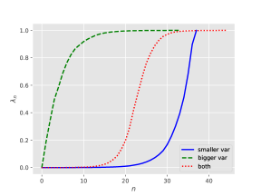
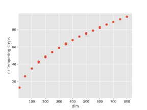
Figure 2: Left: adapted tempering sequences for different $\Sigma$. Right: Length of tempering sequence as a function of $d$ in scenario (a); one recovers the $\mathcal{O}(d^{1/2})$ scaling.

We conclude this section on a remark that discusses about related adaptive tempering strategies.

Remark 1.

Proposition 1 provides alternative methods to approximately solve $\chi^{2}(\mu_{n-1}|\mu_{n})=\beta$ in a equivalent way (up to higher order terms) from the current set of particles. A first one is to fix to a constant:

$$\mathop{\mathrm{KL}}\nolimits(\mu_{n-1}|\mu_{n})\approx-\frac{1}{N}\sum_{i=1}^{N}\log w_{n}(\widetilde{X}_{n-1}^{i})+\log\frac{1}{N}\sum_{i=1}^{N}w_{n}(\widetilde{X}_{n-1}^{i}),$$

which is likely to be more stable than the ESS, since it involves the log-weights rather than the weights themselves. The second one is set the next $\lambda_{n}$ as $\lambda_{n}=\lambda_{n-1}+(\beta/\hat{\mathrm{I}}(\lambda_{n-1}))^{1/2}$, where $\hat{\mathrm{I}}(\lambda_{n-1})$ is

$$\frac{1}{N}\sum_{i=1}^{N}\left(\log\frac{\pi(\widetilde{X}_{n-1}^{i})}{\mu_{0}(\widetilde{X}_{n-1}^{i})}\right)^{2}-\left(\frac{1}{N}\sum_{i=1}^{N}\log\frac{\pi(\widetilde{X}_{n-1}^{i})}{\mu_{0}(\widetilde{X}_{n-1}^{i})}\right)^{2}.$$

5 Related work

In this section we discuss alternative tempering strategies and algorithmic approximations related to the tempering update.

Connection between tempering and KL divergence optimization. The connection between the tempered distribution (13) and the KL divergence has also been studied in Grosse et al., (2013), which shows that

$$\mu_{\lambda}=\arg\min_{\mu}\left[(1-\lambda)\mathop{\mathrm{KL}}\nolimits(\mu|\mu_{0})+\lambda\mathop{\mathrm{KL}}\nolimits(\mu|\pi)\right].$$

This corresponds to the first step of entropic mirror descent, i.e. (3) with $n=0$ and $\lambda=\gamma_{1}$. More recently, Goshtasbpour et al., (2023) also highlighted a connection between the tempering sequence and KL optimization. In their Proposition 3.2 they show that the tempering sequence is the path of steepest descent for the KL; i.e. that minimizes (1) infinitesimally, where the perturbation $\xi$ is a smooth ($C^{1}$) perturbation with bounded variance; integrating such a path yields the tempering sequence. From there, they identify a tempering schedule that decreases the KL divergence with constant rate and satisfies the ODE

$$\dot{\lambda}=c\left[\mathrm{I}(\lambda)(1-\lambda)\right]^{-1}$$ (20)

This differs from ours in (16) that states that $\lambda(t)$ should satisfy $\dot{\lambda}=c\mathrm{I}(\lambda)^{-1/2}$. Both strategies can be justified using the well known identity (Brekelmans et al., 2020b, , Section 4.4)

$$\mathop{\mathrm{KL}}\nolimits(\mu_{\lambda}|\mu_{\lambda^{\prime}}) =\int_{\lambda}^{\lambda^{\prime}}(\lambda-u)\mathrm{I}(u)du.$$

The ODE (20) seeks the tempering schedule of steepest descent for $\mathop{\mathrm{KL}}\nolimits(\mu_{\lambda}|\pi)$, while (16) keeps the $\mathop{\mathrm{KL}}\nolimits$ between successive entropic mirror descent iterates constant, which results in convenient simplifying terms. Further details are given in Appendix C.

Effect of the dimension on tempering/SMC in Beskos et al., (2014). In this paper the authors investigate the effect of dimension on the stability of SMC methods. There, stability refers to the ability of the SMC algorithm to produce accurate approximations of the target distribution as the dimension increases, while keeping the computational cost reasonable. The authors show that for a certain class of target densities (an i.i.d. target of the form $\pi(x)=\prod_{i=1}^{d}\pi^{i}(x^{i})$ where $x=(x^{1},\dots,x^{d})\in\mathbb{R}^{d}$), SMC with the tempering sequence defined as $\lambda_{n}=\lambda_{1}+\nicefrac{{(n-1)(1-\lambda_{1})}}{{d}}$, $1\leq n\leq d$, is stable, i.e. the ESS converges weakly to a non-trivial limit ($\textrm{ESS}\in(1,N)$) as $d$ grows and the number of particles is kept fixed. This result suggests using $\mathcal{O}(d)$ tempering iterations contrary to the $\mathcal{O}(d^{1/2})$ found in Proposition 1 and confirmed by our numerical results. We leave further investigation of the optimal scaling with $d$ of SMC samplers for future work.

Parallel tempering. The tempering iterates (10) are also at the basis of Parallel Tempering (PT) (Geyer,, 1991; Hukushima and Nemoto,, 1996), a class of Markov chain Monte Carlo algorithms which relies on interacting Markov chains to sample from (10). PT is not based on importance sampling, hence the connection with Mirror Descent is less clear since identifying an update of the form (17) is not possible. It is customary in PT (Syed et al.,, 2022, e.g. Section 4) to fix the tempering sequences so that the acceptance probability of a swap between two successive $\lambda_{n}$ is constant in $n$. One may use Proposition 1 of Predescu et al., (2004), see also Theorem 2 in Syed et al., (2022), which is similar in spirit to our Proposition 1, but not equivalent: Proposition 1 applies to the $f$ divergence between $\mu_{\lambda}$ and $\mu_{\lambda^{\prime}}$, for $\lambda^{\prime}\approx\lambda$, where $f$ is differentiable, whereas the acceptance rate of a PT swap is the TV distance between $\mu_{\lambda}\otimes\mu_{\lambda^{\prime}}$ and $\mu_{\lambda^{\prime}}\otimes\mu_{\lambda}$, again for $\lambda^{\prime}\approx\lambda$.

Adaptive tempering. In Korba and Portier, (2022), the authors propose to choose the step-size $\gamma_{n}$ as follows. At time $n$ draw $m_{n}$ particles from $q_{n}^{\textrm{SRAIS}}$. Let $P=\sum_{l=1}^{m_{n}}u_{n}^{l}\delta_{X_{n}^{l}}$ and $Q=\sum_{l=1}^{m_{n}}\nicefrac{{1}}{{m_{n}}}\delta_{X_{n}^{l}}$ the reweighted and uniform distribution on the particles $(X_{n}^{l})_{l=1}^{m_{n}}$ respectively, where $u_{n}^{l}=u_{n}(X_{n}^{l})=\pi(x)/q_{n}(x)$ are the importance weights between the target distribution $\pi$ and the current approximate iterate $q_{n}$ of $\mu_{n}$. Korba and Portier, (2022) propose to set $\gamma_{n}$ as $\gamma_{n}=1-R_{\alpha}(P|Q)/\log(m_{n})$, where $R_{\alpha}$ is Renyi’s $\alpha$-divergence (Rényi et al.,, 1961) of $P$ from $Q$, in particular $R_{1}(P||Q)=\mathop{\mathrm{KL}}\nolimits(P|Q)$, and $\log(m_{n})$ normalizes the ratio between 0 and 1. Hence, for $\alpha=1$ and without the discrete particle approximation, their rule can be written $\gamma_{n}=1-\mathop{\mathrm{KL}}\nolimits(\mu_{n}|\pi).$ Since $\gamma_{n}=(\lambda_{n}-\lambda_{n-1})/(1-\lambda_{n-1})$, by the decrease of KL formula (14), this rule can also be seen as enforcing a gap between consecutive $\lambda$’s as a constant.

Mini-batching. When the target $\pi$ is the posterior distribution of a large dataset, one may combine mirror descent with mini-batching strategies, as suggested in Dai et al., (2016). In the context of SMC samplers, one may combine tempering with the IBIS strategy of Chopin, (2002) to obtain a tempered IBIS SMC sampler, where one may divide the dataset in $k$ batches, use tempering SMC recursively to progress from the prior to $\pi$ given the first batch, then from that posterior to the posterior given the first two batches, and so on.

6 Conclusions

This paper establishes a connection between entropic mirror descent and tempering to sample from a target probability distribution known up to a normalizing constant. We show that the two strategies are equivalent under some conditions on the step-sizes of mirror descent $(\gamma_{n})_{n\geq 0}$ and the tempering sequence $(\lambda_{n})_{n=0}^{T}$ and obtain an explicit convergence rate in terms of $\lambda_{n}$ for the tempering iterates. Provided one can obtain an approximation of $\mathop{\mathrm{KL}}\nolimits(\pi|\mu_{0})$ (using, for example Proposition 1 with $f(x)=-\log x,\lambda=1,\lambda^{\prime}=0$), we can infer the value of $\lambda_{n}$ necessary to guarantee that the $n-$th tempering iterate is sufficiently close to $\pi$. We provide an optimization point of view on sequential Monte Carlo (and other algorithms based on importance sampling) and motivate the adaptive strategy commonly used in the literature through mirror descent. Furthermore, we identify that for a number of algorithms based on importance sampling, the importance weights carry the gradient information, and propose strategies to reduce their numerical error (see Appendix D). This paper focuses on minimization of the KL divergence, however other divergences could be considered (e.g. $\alpha$-divergences). We leave this direction and its connection with alternative tempering sequences (Brekelmans et al., 2020a, ; Goshtasbpour et al.,, 2023) for future work.

Appendix A Proof of (8)

The proof below is written for a generic $L$-smooth and $l$-strongly convex functional $\mathcal{F}$ relatively to a Bregman potential $\phi$. Recall that in the case of $\mathcal{F}$ being the Kullback-Leibler divergence and negative entropy, $L=l=1$.

We first state a preliminary result, known as the "three-point inequality" or "Bregman proximal inequality", which can be found in (Aubin-Frankowski et al.,, 2022, Lemma 3).

Lemma 1 (Three-point inequality).

Given $\mu\in\mathcal{M}(\mathbb{R}^{d})$ and some proper convex functional $\mathcal{G}:\mathcal{M}(\mathbb{R}^{d})\rightarrow\mathbb{R}\cup\{+\infty\}$, if $\nabla\phi(\mu)$ exists, as well as $\bar{\nu}=\operatorname*{argmin}_{\nu\in C}\{\mathcal{G}(\nu)+D_{\phi}(\nu|\mu)\}$, then for all $\nu\in C\cap\operatorname*{dom}(\phi)\cap\operatorname*{dom}(\mathcal{G})$:

$$\mathcal{G}(\nu)+D_{\phi}(\nu|\mu)\geq\mathcal{G}(\bar{\nu})+D_{\phi}(\bar{\nu}|\mu)+D_{\phi}(\nu|\bar{\nu}).$$ (21)

We can now start the proof of mirror descent convergence rate. Since $\mathcal{F}$ is $L$-smooth relative to $\phi$ and $\gamma_{n+1}<1/L$ implies, we have

$$\mathcal{F}(\mu_{n+1}) \leq\mathcal{F}(\mu_{n})+\langle\nabla\mathcal{F}(\mu_{n}),\mu_{n+1}-\mu_{n}\rangle+LD_{\phi}(\mu_{n+1}|\mu_{n})$$ (22)

$$\leq\mathcal{F}(\mu_{n})+\langle\nabla\mathcal{F}(\mu_{n}),\mu_{n+1}-\mu_{n}\rangle+\frac{1}{\gamma_{n+1}}D_{\phi}(\mu_{n+1}|\mu_{n}).$$

Applying Lemma 1 to the convex function $\mathcal{G}_{n}(\nu)=\gamma_{n+1}\langle\nabla\mathcal{F}(\mu_{n}),\nu-\mu_{n}\rangle$, with $\mu=\mu_{n}$ and $\bar{\nu}=\mu_{n+1}$ yields

$$\langle\nabla\mathcal{F}(\mu_{n}),\mu_{n+1}-\mu_{n}\rangle+\frac{1}{\gamma_{n+1}}D_{\phi}(\mu_{n+1}|\mu_{n})\leq\langle\nabla\mathcal{F}(\mu_{n}),\nu-\mu_{n}\rangle+\frac{1}{\gamma_{n+1}}D_{\phi}(\nu|\mu_{n})-\frac{1}{\gamma_{n+1}}D_{\phi}(\nu|\mu_{n+1}).$$

Fix $\nu$, then (22) becomes:

$$\mathcal{F}(\mu_{n+1})\leq\mathcal{F}(\mu_{n})+\langle\nabla\mathcal{F}(\mu_{n}),\nu-\mu_{n}\rangle+\frac{1}{\gamma_{n+1}}D_{\phi}(\nu|\mu_{n})-\frac{1}{\gamma_{n+1}}D_{\phi}(\nu|\mu_{n+1}).$$ (23)

This shows in particular, by substituting $\nu=\mu_{n}$ and since $D_{\phi}(\nu|\mu_{n+1})\geq 0$, that

$$\mathcal{F}(\mu_{n+1})\leq\mathcal{F}(\mu_{n})-\frac{1}{\gamma_{n+1}}D_{\phi}(\mu_{n}|\mu_{n+1}),$$ (24)

i.e. $\mathcal{F}$ is decreasing at each iteration. Since $\mathcal{F}$ is $l$-strongly convex relative to $\phi$, we also have:

$$\langle\nabla\mathcal{F}(\mu_{n}),\nu-\mu_{n}\rangle\leq\mathcal{F}(\nu)-\mathcal{F}(\mu_{n})-lD_{\phi}(\nu|\mu_{n})$$

and (23) becomes:

$$\mathcal{F}(\mu_{n+1})\leq\mathcal{F}(\nu)+\left(\frac{1}{\gamma_{n+1}}-l\right)D_{\phi}(\nu|\mu_{n})-\frac{1}{\gamma_{n+1}}D_{\phi}(\nu|\mu_{n+1}),$$ (25)

i.e., multiplying the previous equation by $(\gamma_{n+1}^{-1}-l)^{-1}$, we get

$$\left(\frac{1}{1-\gamma_{n+1}l}\right)\mathcal{F}(\mu_{n+1})\leq\left(\frac{1}{1-\gamma_{n+1}l}\right)\mathcal{F}(\nu)+\frac{1}{\gamma_{n+1}}D_{\phi}(\nu|\mu_{n})-\frac{1}{\gamma_{n+1}}\left(\frac{1}{1-\gamma_{n+1}l}\right)D_{\phi}(\nu|\mu_{n+1}).$$ (26)

A.1 Proof for $(\gamma_{n})_{n\geq 1}$ decreasing or constant

Similarly to Lu et al., (2018), we now consider for $n\geq 1$:

$$\mathcal{P}(n):\quad\sum_{k=1}^{n}\left(\frac{1}{1-\gamma_{k}l}\right)^{k}\mathcal{F}(\mu_{k})\leq\sum_{k=1}^{n}\left(\frac{1}{1-\gamma_{k}l}\right)^{k}\mathcal{F}(\nu)+\frac{1}{\gamma_{1}}D_{\phi}(\nu|\mu_{0})-\frac{1}{\gamma_{n}}\left(\frac{1}{1-\gamma_{n}l}\right)^{n}D_{\phi}(\nu|\mu_{n}).$$

We first have that

$$\mathcal{P}(1):\left(\frac{1}{1-\gamma_{1}l}\right)\mathcal{F}(\mu_{1})\leq\left(\frac{1}{1-\gamma_{1}l}\right)\mathcal{F}(\nu)+\frac{1}{\gamma_{1}}D_{\phi}(\nu|\mu_{0})-\frac{1}{\gamma_{1}}\left(\frac{1}{1-\gamma_{1}l}\right)D_{\phi}(\nu|\mu_{1})$$

is true by (26). Then, assume $\mathcal{P}(n)$ holds. We have by (26):

$$\sum_{k=1}^{n+1}\left(\frac{1}{1-\gamma_{k}l}\right)^{k}\mathcal{F}(\mu_{k})=\sum_{k=1}^{n}\left(\frac{1}{1-\gamma_{k}l}\right)^{k}\mathcal{F}(\mu_{k})+\left(\frac{1}{1-\gamma_{n+1}l}\right)^{n+1}\mathcal{F}(\mu_{n+1})\\ \leq\sum_{k=1}^{n}\left(\frac{1}{1-\gamma_{k}l}\right)^{k}\mathcal{F}(\nu)+\frac{1}{\gamma_{1}}D_{\phi}(\nu|\mu_{0})-\frac{1}{\gamma_{n}}\left(\frac{1}{1-\gamma_{n}l}\right)^{n}D_{\phi}(\nu|\mu_{n})\\ +\left(\frac{1}{1-\gamma_{n+1}l}\right)^{n+1}\mathcal{F}(\nu)+\frac{1}{\gamma_{n+1}}\left(\frac{1}{1-\gamma_{n+1}l}\right)^{n}D_{\phi}(\nu|\mu_{n})-\frac{1}{\gamma_{n+1}}\left(\frac{1}{1-\gamma_{n+1}l}\right)^{n+1}D_{\phi}(\nu|\mu_{n+1})\\ \leq\sum_{k=1}^{n+1}\left(\frac{1}{1-\gamma_{k}l}\right)^{k}\mathcal{F}(\nu)+\frac{1}{\gamma_{1}}D_{\phi}(\nu|\mu_{0})-\frac{1}{\gamma_{n+1}}\left(\frac{1}{1-\gamma_{n+1}l}\right)^{n+1}D_{\phi}(\nu|\mu_{n+1})$$

where we used in the last inequality (to upper bound the sum of the third and fifth term by zero) that $s\mapsto s^{-1}(1-s)^{-n}$ was a monotone increasing function and that the sequence $(\gamma_{n})_{n\geq 1}$ was decreasing, showing $\mathcal{P}(n+1)$ holds. Hence $\mathcal{P}(n)$ is true for all $n\geq 1$. Then, using the monotonicity of $(\mathcal{F}(\mu_{n}))_{n\geq 0}$ on the left hand side and the positivity of $D_{\phi}(\nu|\mu_{n})$ on the right hand side of $\mathcal{P}(n)$, we have

$$\sum_{k=1}^{n}\left(\frac{1}{1-\gamma_{k}l}\right)^{k}\left(\mathcal{F}(\mu_{n})-\mathcal{F}(\nu)\right)\leq\frac{1}{\gamma_{1}}D_{\phi}(\nu|\mu_{0})-\frac{1}{\gamma_{n}}\left(\frac{1}{1-\gamma_{n}l}\right)^{n}D_{\phi}(\nu|\mu_{n})\leq\frac{1}{\gamma_{1}}D_{\phi}(\nu|\mu_{0}).$$

This shows that

$$\mathcal{F}(\mu_{n})-\mathcal{F}(\mu)\leq\frac{C_{n}}{\gamma_{1}}D_{\phi}(\nu|\mu_{0}),\text{ where }C_{n}^{-1}=\sum_{k=1}^{n}\left(\frac{1}{1-\gamma_{k}l}\right)^{k}.$$

A.2 Proof for general $(\gamma_{n})_{n\geq 1}$

Consider for $n\geq 1$:

$$\mathcal{P}(n):\quad\sum_{k=1}^{n}\frac{\gamma_{k}}{\gamma_{1}}\prod_{i=1}^{k}\frac{1}{1-\gamma_{i}l}\mathcal{F}(\mu_{k})\leq\sum_{k=1}^{n}\frac{\gamma_{k}}{\gamma_{1}}\prod_{i=1}^{k}\frac{1}{1-\gamma_{i}l}\mathcal{F}(\nu)+\frac{1}{\gamma_{1}}D_{\phi}(\nu|\mu_{0})-\frac{1}{\gamma_{1}}\prod_{i=1}^{n}\frac{1}{1-\gamma_{i}l}D_{\phi}(\nu|\mu_{n})$$

We first have that

$$\mathcal{P}(1):\left(\frac{1}{1-\gamma_{1}l}\right)\mathcal{F}(\mu_{1})\leq\left(\frac{1}{1-\gamma_{1}l}\right)\mathcal{F}(\nu)+\frac{1}{\gamma_{1}}D_{\phi}(\nu|\mu_{0})-\frac{1}{\gamma_{1}}\left(\frac{1}{1-\gamma_{1}l}\right)D_{\phi}(\nu|\mu_{1})$$

is true by (26). Then, assume $\mathcal{P}(n)$ holds. We have by (26):

$$\sum_{k=1}^{n+1}\frac{\gamma_{k}}{\gamma_{1}}\prod_{i=1}^{k}\frac{1}{1-\gamma_{i}l}\mathcal{F}(\mu_{k})=\sum_{k=1}^{n}\frac{\gamma_{k}}{\gamma_{1}}\prod_{i=1}^{k}\frac{1}{1-\gamma_{i}l}\mathcal{F}(\mu_{k})+\frac{\gamma_{n+1}}{\gamma_{1}}\prod_{i=1}^{n+1}\frac{1}{1-\gamma_{i}l}\mathcal{F}(\mu_{n+1})\\ \leq\sum_{k=1}^{n}\frac{\gamma_{k}}{\gamma_{1}}\prod_{i=1}^{k}\frac{1}{1-\gamma_{i}l}\mathcal{F}(\nu)+\frac{1}{\gamma_{1}}D_{\phi}(\nu|\mu_{0})-\frac{1}{\gamma_{1}}\prod_{i=1}^{n}\frac{1}{1-\gamma_{i}l}D_{\phi}(\nu|\mu_{n})\\ +\frac{\gamma_{n+1}}{\gamma_{1}}\prod_{i=1}^{n}\frac{1}{1-\gamma_{i}l}\left(\left(\frac{1}{1-\gamma_{n+1}l}\right)\mathcal{F}(\nu)+\frac{1}{\gamma_{n+1}}D_{\phi}(\nu|\mu_{n})-\frac{1}{\gamma_{n+1}}\left(\frac{1}{1-\gamma_{n+1}l}\right)D_{\phi}(\nu|\mu_{n+1})\right)\\ =\sum_{k=1}^{n+1}\frac{\gamma_{k}}{\gamma_{1}}\prod_{i=1}^{k}\frac{1}{1-\gamma_{i}l}\mathcal{F}(\nu)+\frac{1}{\gamma_{1}}D_{\phi}(\nu|\mu_{0})-\frac{1}{\gamma_{1}}\prod_{i=1}^{n+1}\frac{1}{1-\gamma_{i}l}D_{\phi}(\nu|\mu_{n+1}),$$

showing $\mathcal{P}(n+1)$ holds. Hence $\mathcal{P}(n)$ is true for all $n\geq 1$. Then, using the monotonicity of $(\mathcal{F}(\mu_{n}))_{n\geq 0}$ on the left hand side and the positivity of $D_{\phi}(\nu|\mu_{n})$ on the right hand side of $\mathcal{P}(n)$, we have

$$\sum_{k=1}^{n}\frac{\gamma_{k}}{\gamma_{1}}\prod_{i=1}^{k}\frac{1}{1-\gamma_{i}l}\left(\mathcal{F}(\mu_{n})-\mathcal{F}(\nu)\right)\leq\frac{1}{\gamma_{1}}D_{\phi}(\nu|\mu_{0})-\frac{1}{\gamma_{1}}\prod_{i=1}^{n}\frac{1}{1-\gamma_{i}l}D_{\phi}(\nu|\mu_{n})\leq\frac{1}{\gamma_{1}}D_{\phi}(\nu|\mu_{0}).$$

This shows that

$$\mathcal{F}(\mu_{n})-\mathcal{F}(\mu)\leq\frac{C_{n}}{\gamma_{1}}D_{\phi}(\nu|\mu_{0}),\text{ where }C_{n}^{-1}=\sum_{k=1}^{n}\frac{\gamma_{k}}{\gamma_{1}}\prod_{i=1}^{k}\frac{1}{1-\gamma_{i}l}.$$

In particular for $l=1$ and $\gamma_{k}=(\lambda_{k}-\lambda_{k-1})/(1-\lambda_{k-1})$,

$$C_{n}^{-1}=\frac{1}{\lambda_{1}}\sum_{k=1}^{n}\left(\frac{\lambda_{k}-\lambda_{k-1}}{1-\lambda_{k-1}}\frac{1-\lambda_{0}}{1-\lambda_{k}}\right)=\frac{1}{\lambda_{1}}\sum_{k=1}^{n}\left(\frac{\lambda_{k}-\lambda_{k-1}}{(1-\lambda_{k-1})(1-\lambda_{k})}\right),$$

where we used $\lambda_{0}=0$.

A.3 Bounds on convergence rate

In this section we prove upper bounds on the convergence rates previously obtained. Our bounds are obtained in the case $l=1$ and $\gamma_{n}\leq 1/L=1$ for all $n\geq 1$.

We show that

$$C_{n}=\left(\sum_{k=1}^{n}\frac{\gamma_{k}}{\gamma_{1}}\prod_{i=1}^{k}\frac{1}{1-\gamma_{i}}\right)^{-1}\leq\prod_{k=1}^{n}(1-\gamma_{k}).$$ (27)

To see this we consider for $n\geq 1$, $\mathcal{P}(n):\quad\sum_{k=1}^{n}\frac{\gamma_{k}}{\gamma_{1}}\prod_{i=1}^{k}\frac{1}{1-\gamma_{i}}\geq\prod_{k=1}^{n}(1-\gamma_{k})^{-1}$. We trivially have that $\mathcal{P}(1):\left(\frac{1}{1-\gamma_{1}}\right)^{1}\geq(1-\gamma_{1})^{-1}$ is true. Then, assume $\mathcal{P}(n)$ holds. We have

$$\sum_{k=1}^{n+1}\frac{\gamma_{k}}{\gamma_{1}}\prod_{i=1}^{k}\frac{1}{1-\gamma_{i}}=\sum_{k=1}^{n}\frac{\gamma_{k}}{\gamma_{1}}\prod_{i=1}^{k}\frac{1}{1-\gamma_{i}}+\frac{\gamma_{n+1}}{\gamma_{1}}\prod_{i=1}^{n+1}\frac{1}{1-\gamma_{i}}\geq\prod_{k=1}^{n}(1-\gamma_{k})^{-1}+\gamma_{n+1}\prod_{k=1}^{n+1}(1-\gamma_{k})^{-1}\\ =\prod_{k=1}^{n}(1-\gamma_{k})^{-1}\left[1+\gamma_{n+1}(1-\gamma_{n+1})^{-1}\right]=\prod_{k=1}^{n+1}(1-\gamma_{k})^{-1}$$

since $\gamma_{1}\leq 1$ for all $n\geq 1$, showing $\mathcal{P}(n+1)$ holds. Hence (27) is true for all $n\geq 1$.

Appendix B Proof of Proposition 1

B.1 Tempering sequence as a parametric model

Let us recall that the tempering sequence is defined as:

$$\mu_{\lambda}(x)=\frac{\mu_{0}^{1-\lambda}(x)\pi^{\lambda}(x)}{\exp\left\{\psi(\lambda)\right\}}=\mu_{0}(x)\exp\left\{\lambda s(x)-\psi(\lambda)\right\}$$

for $\lambda\in[0,1]$, where $s(x):=\log\pi(x)/\mu_{0}(x)$, and

$$\psi(\lambda):=\log\int\mu_{0}(x)\exp\left\{\lambda s(x)\right\}dx$$

is the partition function (log-normalizing constant).

In our case, the score is: $t_{\lambda}(x)=s(x)-\psi^{\prime}(\lambda)$ (the score has expectation zero, as expected since $\psi^{\prime}(\lambda)=\mathbb{E}_{\lambda}[s(X)]$), and

$$I(\lambda):=\mathrm{Var}_{\lambda}\left[t_{\lambda}(X)\right]=\mathbb{E}_{\lambda}\left[t_{\lambda}(X)^{2}\right]=\mathrm{Var}_{\lambda}\left[s(X)\right].$$

Note also the well-known identity:

$$I(\lambda)=-\mathbb{E}_{\lambda}[t^{\prime}_{\lambda}(X)]=-\mathbb{E}_{\lambda}\left[\frac{\partial^{2}\log\mu_{\lambda}(X)}{\partial\lambda^{2}}\right].$$

B.2 Proof

Recall that $f$ must be convex and such that $f(1)=0$.

By the standard properties of $f-$divergence, it is clear that the function $\varphi_{\lambda}:$ $\lambda^{\prime}\rightarrow D_{f}(\lambda,\lambda^{\prime})$ is non-negative, and zero at $\lambda^{\prime}=\lambda$, hence its first derivative must be zero at $\lambda^{\prime}=\lambda$. In fact,

$$\varphi^{\prime}_{\lambda}(\lambda^{\prime}) =\int\mu_{\lambda^{\prime}}^{\prime}f^{\prime}(\mu_{\lambda^{\prime}}/\mu_{\lambda})=\int\mu_{\lambda^{\prime}}t_{\lambda^{\prime}}f^{\prime}(\mu_{\lambda^{\prime}}/\mu_{\lambda})$$

and note we have indeed $\varphi^{\prime}_{\lambda}(\lambda)=f^{\prime}(1)\int\mu_{\lambda}^{\prime}=0$. For the second derivative

$$\varphi^{\prime\prime}_{\lambda}(\lambda^{\prime})=\int\mu_{\lambda^{\prime}}(t_{\lambda^{\prime}}^{\prime}+t_{\lambda^{\prime}}^{2})f^{\prime}\left(\frac{\mu_{\lambda^{\prime}}}{\mu_{\lambda}}\right)+\int\frac{\left(\mu_{\lambda^{\prime}}t_{\lambda^{\prime}}\right)^{2}}{\mu_{\lambda}}f^{\prime\prime}\left(\frac{\mu_{\lambda^{\prime}}}{\mu_{\lambda}}\right)$$

and at $\lambda^{\prime}=\lambda$:

$$\varphi^{\prime\prime}_{\lambda}(\lambda) =f^{\prime}(1)\int\mu_{\lambda}(t_{\lambda}^{\prime}+t_{\lambda}^{2})+f^{\prime\prime}(1)\int\mu_{\lambda}\left(t_{\lambda}\right)^{2}$$

$$=f^{\prime\prime}(1)I(\lambda).$$

This ends the proof.

Appendix C Further discussion on (20)

Consider the well-known identity Brekelmans et al., 2020b (, Section 4.4)

$$\mathop{\mathrm{KL}}\nolimits(\mu_{\lambda_{n-1}}|\mu_{\lambda_{n}}) =\int_{\lambda_{n-1}}^{\lambda_{n}}(\lambda_{n}-\lambda)\mathrm{Var}_{\lambda}\left[s(X)\right]d\lambda$$ (28)

$$=\int_{\lambda_{n-1}}^{\lambda_{n}}(\lambda_{n}-\lambda)\mathrm{I}(\lambda)d\lambda.$$

We want to study the infinitesimal behaviour of the $\mathop{\mathrm{KL}}\nolimits$ when $\lambda_{n-1}=\lambda(t)$ but $\lambda_{n}$ is fixed. As suggested in Goshtasbpour et al., (2023) a natural requirement is to keep the derivative of the $\mathop{\mathrm{KL}}\nolimits$ w.r.t. time constant

$$\frac{d}{dt}\mathop{\mathrm{KL}}\nolimits(\mu_{\lambda(t)}|\mu_{\lambda_{n}}) =\frac{d}{dt}\left(\int_{\lambda(t)}^{\lambda_{n}}(\lambda_{n}-\lambda)\mathrm{I}(\lambda)d\lambda\right)$$

$$=\frac{d\lambda(t)}{dt}(\lambda_{n}-\lambda(t))\mathrm{I}(\lambda(t))=c,$$

where we used Leibniz integral rule for differentiation under the integral sign under the assumptions that all quantities are well-defined. This gives us the following ODE for $\lambda(t)$

$$\frac{d\lambda(t)}{dt}=c\left[(\lambda_{n}-\lambda(t))\mathrm{I}(\lambda(t))\right]^{-1}.$$ (29)

If we set $\lambda_{n}=1$, i.e. we want to decrease the $\mathop{\mathrm{KL}}\nolimits$ between $\mu_{\lambda(t)}$ and $\pi$ at a constant rate we obtain

$$\frac{d\lambda(t)}{dt}=c\left[(1-\lambda(t))\mathrm{I}(\lambda(t))\right]^{-1},$$

i.e. the ODE given in Goshtasbpour et al., (2023), where we used the fact that

$$\textrm{Var}_{\mu_{\lambda(t)}}\left(\log(\frac{\pi}{\mu_{\lambda(t)}}(x))\right)=(1-\lambda(t))^{2}\textrm{Var}_{\mu_{\lambda(t)}}\left(\log(\frac{\pi}{\mu_{0}}(x))\right)=(1-\lambda(t))^{2}\mathrm{I}(\lambda(t)).$$

If we instead assume that $\lambda_{n}$ is sufficiently close to $\lambda(t)$ that $\lambda_{n}-\lambda(t)\approx\nicefrac{{d\lambda(t)}}{{dt}}$ we obtain the ODE in (16). Or, equivalently, by discretizing (29) we obtain

$$\lambda_{n}-\lambda_{n-1}=c\left[(\lambda_{n}-\lambda_{n-1})\mathrm{I}(\lambda_{n-1})\right]^{-1},$$

which is equivalent to (15).

Appendix D Algorithms details

We collect here further details on the SMC samplers described in Section 4 and describe other strategies based on importance sampling that approximate the mirror descent iterates (6).

1:  Inputs: sequences of temperatures $(\lambda_{n})_{n=1}^{T}$, Markov kernels $(M_{n})_{n=1}^{T}$, initial proposal $\mu_{0}$.

2:  Initialize: set $\lambda_{0}=0$, sample $\widetilde{X}_{0}^{i}\sim\mu_{0}$ and set $W_{0}^{i}=1/N$ for $i=1,\dots,N$.

3:  for $n=1,\dots,T$ do

4:     if $n>1$ then

5:        Resample: draw $\{\widetilde{X}_{n-1}^{i}\}_{i=1}^{N}$ independently from $\{X_{n-1}^{i},W_{n-1}^{i}\}_{i=1}^{N}$ and set $W_{n}^{i}=1/N$ for $i=1,\dots,N$.

6:     end if

7:     Propose: draw $X_{n}^{i}\sim M_{n}(\cdot,\widetilde{X}_{n-1}^{i})$ for $i=1,\dots,N$.

8:     Reweight: compute and normalize the weights $W_{n}^{i}\propto w_{n}(\widetilde{X}_{n-1}^{i})$ for $i=1,\dots,N$.

9:  end for

10:  Output: $q_{n}(x)=\sum_{i=1}^{N}W_{n}^{i}\delta_{X_{n}^{i}}(x)$

Algorithm 1 SMC samplers (Del Moral et al.,, 2006).

D.1 Other schemes

Particle Mirror Descent (PMD). Similarly to SMC, Dai et al., (2016) propose an approximation of the mirror descent iterates (7) based on importance sampling. The mirror descent iterate at time $n$ is approximated by a kernel density estimator (KDE)

$$q_{n}^{\textrm{PMD}}(x):=\sum_{i=1}^{N}V_{n}^{i}K_{h_{n}}(x-X_{n}^{i}),$$ (30)

where $\{X_{n}^{i},V_{n}^{i}\}_{i=1}^{N}$ denotes a weighted particle set and $K_{h_{n}}$ is a smoothing kernel with bandwidth $h_{n}$. At iteration $n$ the weighted particle set $\{X_{n-1}^{i},V_{n-1}^{i}\}_{i=1}^{N}$ is resampled to obtain the equally weighted particle set $\{\widetilde{X}_{n-1}^{i},1/N\}_{i=1}^{N}$, the kernel $K_{h_{n}}$ is applied to propose new particle locations $X_{n}^{i}\sim K_{h_{n}}(\cdot-\widetilde{X}_{n-1}^{i})$. The weights for the proposed particle set are then proportional to

$$v_{n}(x)=\left(\frac{\pi(x)}{q_{n-1}^{\textrm{PMD}}(x)}\right)^{\gamma_{n}}.$$ (31)

It is then clear that the Particle Mirror Descent (PMD) scheme summarized in Algorithm 2 in the Appendix is of the form (17).

Comparing PMD with SMC and with the vast literature on SMC algorithms (see, e.g., Chopin and Papaspiliopoulos, (2020) for a comprehensive introduction) we find that PMD is an SMC algorithm targeting the sequence of distributions

$$\tilde{\mu}_{n}(x)\propto\int\mu_{n-1}(x^{\prime})K_{h_{n}}(x-x^{\prime})dx^{\prime}\left(\frac{\pi(x)}{\eta_{n-1}(x)}\right)^{\gamma_{n}},$$ (32)

which converges to the mirror descent iterates (7) as $h_{n}\to 0$. The kernel $K_{h_{n}}$ is replacing the $\mu_{n}$-invariant kernel $M_{n}$ as proposal and the importance weights are given by (31). However, PMD is not a standard SMC algorithm, since the weights $v_{n}$ are approximations of the idealized weights $v_{n}^{\star}(x)=\pi(x)/\int K_{h_{n}}(x-x^{\prime})\mu_{n-1}(x^{\prime})dx^{\prime}$ obtained by plugging the KDE $q_{n-1}^{\textrm{PMD}}$ in place of the denominator. Hence PMD uses one more approximation than standard SMC samplers.

Leveraging the connection between mirror descent and tempering established in Section 3, it is easy to see that $v_{n}^{\star}\to w_{n}$ as $h_{n}\to 0$ (see (19)). Hence, we could replace $v_{n}$ with $w_{n}$ in Algorithm 2 to reduce its computational cost and numerical error, since $v_{n}$ requires an $\mathcal{O}(N)$ cost due to the presence of the kernel density estimator $q_{n-1}$, while the cost of $w_{n}$ is $\mathcal{O}(1)$. Nevertheless, this does not lead to an SMC algorithm targeting $\tilde{\mu}_{n}$ (or $\mu_{n}$).

1:  Inputs: sequences of bandwidths $(h_{n})_{n=1,\ldots,T}$, learning rates $(\gamma_{n})_{n=1,\ldots,T}$, initial proposal $\mu_{0}$.

2:  Initialize: sample $\widetilde{X}_{0}^{i}\sim\mu_{0}$ and set $W_{0}^{i}=1/N$ for $i=1,\dots,N$.

3:  for $n=1,\dots,T$ do

4:     if $n>1$ then

5:        Resample: draw $\{\widetilde{X}_{n-1}^{i}\}_{i=1}^{N}$ independently from $\{X_{n-1}^{i},V_{n-1}^{i}\}_{i=1}^{N}$ and set $V_{n}^{i}=1/N$ for $i=1,\dots,N$.

6:     end if

7:     Propose: draw $X_{n}^{i}\sim K_{h_{n}}(\cdot-\widetilde{X}_{n-1}^{i})$ for $i=1,\dots,N$.

8:     Reweight: compute and normalize the weights $V_{n}^{i}\propto v_{n}(X_{n}^{i})$ for $i=1,\dots,N$.

9:  end for

10:  Output: $q_{n}(x)=\sum_{i=1}^{N}V_{n}^{i}K_{h_{n}}(x-X_{n}^{i})$.

Algorithm 2 Particle Mirror Descent (PMD; Dai et al., (2016)).

Safe and Regularized Adaptive Importance Sampling (SRAIS). Korba and Portier, (2022)) propose an algorithm detailed in Algorithm 3 in the Appendix, that samples at each iteration a particle $X_{n}$ from a proposal $q_{n}^{\textrm{SRAIS}}$. Similarly to PMD which relies on the KDE estimator (30), SRAIS relies on a KDE estimate to approximate the mirror descent iterates

$$q_{n}^{\textrm{SRAIS}}(x)=\sum_{i=1}^{n}U_{i}K_{h_{i}}(x-X_{i}),$$ (33)

where $\{X_{i},U_{i}\}_{i=1}^{n}$ denotes a weighted particle set. However, in this case the size of the particle population is not fixed and the KDE estimate uses all particles from previous iterations. Notice that the particle sampling step (Step 4 of Algorithm 3) can be repeated, resulting in sampling a batch $m_{n}$ of particles at step $n$. The weights for the proposed particles are

$$u_{n}(x)=\left(\frac{\pi(x)}{q_{n-1}^{\textrm{SRAIS}}(x)}\right)^{\gamma_{n}},$$ (34)

and we can identify SRAIS to be of the form (17). Similarly to PMD, one could replace $u_{n}$ with $w_{n}$ in SRAIS.

Remark 2.

In the original scheme proposed by Korba and Portier, (2022), the proposal at each iteration is defined as $\tilde{q}_{n+1}=(1-r_{n+1})q_{n+1}+r_{n+1}q_{0}$ where $q_{n+1}$ is the KDE (33), $(r_{n})_{n\geq 0}$ is a sequence in $[0,1]$ converging to $0$ and $q_{0}$ is a "safe" density (e.g. with heavy tails) preventing the importance weights from degeneracy. In Algorithm 3 we removed the dependency with the safe density and took the sequence $(r_{n})_{n\geq 0}$ constant equal to zero for a clearer presentation.

1:  Inputs: Sequences of bandwidths $(h_{n})_{n=1,\ldots,T}$, learning rates $(\gamma_{n})_{n=1,\ldots,T}$, initial proposal $\mu_{0}$.

2:  Initialize: sample $X_{1}\sim\mu_{0}$ and set $U_{1}=(\pi(X_{1})/\mu_{0}(X_{1}))^{\gamma_{1}}$.

3:  for $n=1,\ldots,T$ do

4:     Propose: draw $X_{n+1}\sim q_{n}$

5:     Reweight: compute the weight $U_{n+1}\propto u_{n+1}(X_{n+1})$ and normalize the weights.

6:     Update the proposal as in (33).

7:  end for

8:  Output: $q_{n+1}(x)=\sum_{i=1}^{n+1}U^{i}K_{h_{i}}(x-X_{i})$.

Algorithm 3 Safe and Regularized Adaptive Importance sampling (SRAIS; Korba and Portier, (2022))

D.2 Comparison of algorithms

As discussed in the previous sections, both SMC samplers and PMD are an instance of SMC algorithms (albeit not a standard one in the case of PMD). The convergence properties of SMC defined in Algorithm 1 are guaranteed by the wide literature on SMC algorithms (see, e.g., Del Moral, (2004) for a complete account). In particular, one can show (see Del Moral, (2004, Theorem 7.4.3) and Crisan and Doucet, (2002)) that every measurable bounded function $\varphi:\mathbb{R}^{d}\to\mathbb{R}$ with $\|\varphi\|:=\sup_{x\in\mathbb{R}^{d}}|\varphi(x)|<\infty$,

$$\mathbb{E}\left[\left\lvert\int\varphi\mathrm{d}\mu_{n}-\int\varphi\mathrm{d}q_{n}^{\textrm{SMC}}\right\rvert\right] \leq\frac{B_{n}^{\textrm{SMC}}\|\varphi\|}{N^{1/2}}$$

where $B_{n}^{\textrm{SMC}}$ denotes a finite constant which does not depend on $N$.

A similar result for Algorithm 2 has been established in Dai et al., (2016, Theorem 5). The approximation error of PMD is divided into an optimisation error, due to the fact that the algorithm is stopped at time $T$, and the following approximation error arising from the particle approximation to the target $\tilde{\mu}_{n}$ in (32)

$$\mathbb{E}\left[\left\lvert\int\varphi\mathrm{d}\tilde{\mu}_{n}-\int\varphi\mathrm{d}q_{n}^{\textrm{PMD}}\right\rvert\right] \leq\frac{B_{n}^{\textrm{PMD}}\|\varphi\|}{N^{1/2}},$$

where $B_{n}^{\textrm{SMC}}$ denotes a finite constant which does not depend on $N$.

In the case of SMC samplers, there is no optimisation error since Algorithm 1 targets $\mu_{n}$ directly (and not the smoothed version (32)) and, by construction, at time $T$ we have $\lambda_{T}=1$ so that $\mu_{T}=\pi$.

Furthermore, when implementing Algorithm 1 there is no need to introduce the kernel $K_{h_{n}}$ to obtain a KDE at each iteration, this results in a simpler algorithm than Algorithm 2 which does not require the bandwidth parameter $h_{n}$ whose tuning is notoriously difficult (Silverman,, 1986). Additionally, KDE performs poorly if the dimension of the underlying space is large (Chacón and Duong,, 2018).

The presence of the KDE in PMD also causes the algorithm to have a higher computational cost than standard SMC samplers, in fact, the presence of the KDE in the weights (31) means that these weights require an $\mathcal{O}(N)$ cost to be computed for each particle, against the $\mathcal{O}(1)$ per particle of the weights (18). These results in a $\mathcal{O}(NT)$ cost for Algorithm 1 and $\mathcal{O}(N^{2}T)$ for Algorithm 2. Clearly, the $\mathcal{O}(N^{2}T)$ of PMD could be reduced to $\mathcal{O}(NT)$ by replacing the weights (31) with (18), since the former are an approximation of the idealized weights $v_{n}^{\star}(x)=(\pi(x)/\mu_{n-1}(x))^{\gamma_{n}}$ which are proportional to (18) as shown in (19), at the cost of targeting a slightly different distribution.

The computational cost of iteration $n$ of SRAIS is $\mathcal{O}(n)$ because of the KDE in the weights (34). Hence, the cost of Algorithm 3 is $\sum_{n=1}^{T}\mathcal{O}(n)\approx\mathcal{O}(T^{2})$. In practice, to reduce computational cost, one could use only the last iterations as the first ones can be considered as “burn-in” steps.

References

- Amari, (2016) Amari, S.-i. (2016). Information Geometry and Its Applications, volume 194. Springer.
- Ambrosio et al., (2008) Ambrosio, L., Gigli, N., and Savaré, G. (2008). Gradient flows: in metric spaces and in the space of probability measures. Springer Science & Business Media.
- Atchadé et al., (2011) Atchadé, Y. F., Roberts, G. O., and Rosenthal, J. S. (2011). Towards optimal scaling of Metropolis-coupled Markov chain Monte Carlo. Statistics and Computing, 21:555–568.
- Aubin-Frankowski et al., (2022) Aubin-Frankowski, P.-C., Korba, A., and Léger, F. (2022). Mirror descent with relative smoothness in measure spaces, with application to Sinkhorn and EM. Advances in Neural Information Processing Systems, 35:17263–17275.
- Beck and Teboulle, (2003) Beck, A. and Teboulle, M. (2003). Mirror descent and nonlinear projected subgradient methods for convex optimization. Operations Research Letters, 31(3):167–175.
- Beskos et al., (2014) Beskos, A., Crisan, D., and Jasra, A. (2014). On the stability of sequential Monte Carlo methods in high dimensions. Annals of Applied Probability, 24(4):1396–1445.
- (7) Brekelmans, R., Masrani, V., Bui, T. D., Wood, F., Galstyan, A., Steeg, G. V., and Nielsen, F. (2020a). Annealed importance sampling with q-paths. In NeurIPS 2020 Workshop: Deep Learning through Information Geometry.
- (8) Brekelmans, R., Masrani, V., Wood, F., Steeg, G. V., and Galstyan, A. (2020b). All in the exponential family: Bregman duality in thermodynamic variational inference. In III, H. D. and Singh, A., editors, Proceedings of the 37th International Conference on Machine Learning, volume 119 of Proceedings of Machine Learning Research, pages 1111–1122. PMLR.
- Chacón and Duong, (2018) Chacón, J. E. and Duong, T. (2018). Multivariate kernel smoothing and its applications. Chapman and Hall/CRC.
- Chizat, (2022) Chizat, L. (2022). Convergence Rates of Gradient Methods for Convex Optimization in the Space of Measures. Open Journal of Mathematical Optimization, 3.
- Chopin, (2002) Chopin, N. (2002). A sequential particle filter method for static models. Biometrika, 89(3):539–551.
- Chopin and Papaspiliopoulos, (2020) Chopin, N. and Papaspiliopoulos, O. (2020). An introduction to sequential Monte Carlo. Springer.
- Crisan and Doucet, (2002) Crisan, D. and Doucet, A. (2002). A survey of convergence results on particle filtering methods for practitioners. IEEE Transactions on Signal Processing, 50(3):736–746.
- Dai et al., (2016) Dai, B., He, N., Dai, H., and Song, L. (2016). Provable Bayesian inference via particle mirror descent. In Artificial Intelligence and Statistics, pages 985–994. PMLR.
- Dai et al., (2022) Dai, C., Heng, J., Jacob, P. E., and Whiteley, N. (2022). An invitation to sequential Monte Carlo samplers. Journal of the American Statistical Association, 117(539):1587–1600.
- Del Moral, (2004) Del Moral, P. (2004). Feynman-Kac formulae: genealogical and interacting particle systems with applications. Probability and Its Applications. Springer Verlag, New York.
- Del Moral et al., (2006) Del Moral, P., Doucet, A., and Jasra, A. (2006). Sequential Monte Carlo samplers. Journal of the Royal Statistical Society Series B: Statistical Methodology, 68(3):411–436.
- Garbuno-Inigo et al., (2020) Garbuno-Inigo, A., Hoffmann, F., Li, W., and Stuart, A. M. (2020). Interacting Langevin diffusions: Gradient structure and ensemble Kalman sampler. SIAM Journal on Applied Dynamical Systems, 19(1):412–441.
- Gelman and Meng, (1998) Gelman, A. and Meng, X.-L. (1998). Simulating normalizing constants: From importance sampling to bridge sampling to path sampling. Statistical Science, pages 163–185.
- Geyer, (1991) Geyer, C. J. (1991). Markov chain Monte Carlo maximum likelihood. In Keramides, E. M., editor, Computing Science and Statistics: Proceedings of the 23rd Symposium on the Interface, pages 156–163.
- Goshtasbpour et al., (2023) Goshtasbpour, S., Cohen, V., and Perez-Cruz, F. (2023). Adaptive annealed importance sampling with constant rate progress. In Krause, A., Brunskill, E., Cho, K., Engelhardt, B., Sabato, S., and Scarlett, J., editors, Proceedings of the 40th International Conference on Machine Learning, volume 202 of Proceedings of Machine Learning Research, pages 11642–11658. PMLR.
- Grosse et al., (2013) Grosse, R. B., Maddison, C. J., and Salakhutdinov, R. R. (2013). Annealing between distributions by averaging moments. In Burges, C., Bottou, L., Welling, M., Ghahramani, Z., and Weinberger, K., editors, Advances in Neural Information Processing Systems, volume 26. Curran Associates, Inc.
- Hukushima and Nemoto, (1996) Hukushima, K. and Nemoto, K. (1996). Exchange Monte Carlo method and application to spin glass simulations. Journal of the Physical Society of Japan, 65(6):1604–1608.
- Jasra et al., (2011) Jasra, A., Stephens, D. A., Doucet, A., and Tsagaris, T. (2011). Inference for Lévy-driven stochastic volatility models via adaptive sequential Monte Carlo. Scandinavian Journal of Statistics, 38(1):1–22.
- Jordan et al., (1998) Jordan, R., Kinderlehrer, D., and Otto, F. (1998). The variational formulation of the Fokker–Planck equation. SIAM Journal on Mathematical Analysis, 29(1):1–17.
- Korba and Portier, (2022) Korba, A. and Portier, F. (2022). Adaptive importance sampling meets mirror descent: a bias-variance tradeoff. In International Conference on Artificial Intelligence and Statistics, pages 11503–11527. PMLR.
- Liu, (2017) Liu, Q. (2017). Stein variational gradient descent as gradient flow. In Guyon, I., Luxburg, U. V., Bengio, S., Wallach, H., Fergus, R., Vishwanathan, S., and Garnett, R., editors, Advances in Neural Information Processing Systems, volume 30. Curran Associates, Inc.
- Lu et al., (2018) Lu, H., Freund, R. M., and Nesterov, Y. (2018). Relatively smooth convex optimization by first-order methods, and applications. SIAM Journal on Optimization, 28(1):333–354.
- Mou et al., (2021) Mou, W., Ma, Y.-A., Wainwright, M. J., Bartlett, P. L., and Jordan, M. I. (2021). High-order Langevin diffusion yields an accelerated MCMC algorithm. The Journal of Machine Learning Research, 22(1):1919–1959.
- Neal, (2001) Neal, R. M. (2001). Annealed importance sampling. Statistics and Computing, 11:125–139.
- Otto and Villani, (2000) Otto, F. and Villani, C. (2000). Generalization of an inequality by Talagrand and links with the logarithmic Sobolev inequality. Journal of Functional Analysis, 173(2):361–400.
- Predescu et al., (2004) Predescu, C., Predescu, M., and Ciobanu, C. V. (2004). The incomplete beta function law for parallel tempering sampling of classical canonical systems. The Journal of Chemical Physics, 120(9):4119–4128.
- Rényi et al., (1961) Rényi, A. et al. (1961). On measures of entropy and information. In Proceedings of the Fourth Berkeley Symposium on Mathematical Statistics and Probability, Volume 1: Contributions to the Theory of Statistics. The Regents of the University of California.
- Roberts and Tweedie, (1996) Roberts, G. O. and Tweedie, R. L. (1996). Exponential convergence of Langevin distributions and their discrete approximations. Bernoulli, pages 341–363.
- Salim et al., (2020) Salim, A., Korba, A., and Luise, G. (2020). The Wasserstein proximal gradient algorithm. Advances in Neural Information Processing Systems, 33:12356–12366.
- Silverman, (1986) Silverman, B. W. (1986). Density Estimation for Statistics and Data Analysis. Chapman & Hall.
- Syed et al., (2022) Syed, S., Bouchard-Côté, A., Deligiannidis, G., and Doucet, A. (2022). Non-reversible parallel tempering: a scalable highly parallel MCMC scheme. Journal of the Royal Statistical Society Series B: Statistical Methodology, 84(2):321–350.
- Syed et al., (2021) Syed, S., Romaniello, V., Campbell, T., and Bouchard-Côté, A. (2021). Parallel tempering on optimized paths. In International Conference on Machine Learning, pages 10033–10042. PMLR.
- Wibisono, (2018) Wibisono, A. (2018). Sampling as optimization in the space of measures: The Langevin dynamics as a composite optimization problem. In Conference on Learning Theory, pages 2093–3027. PMLR.
- Ying, (2020) Ying, L. (2020). Mirror descent algorithms for minimizing interacting free energy. Journal of Scientific Computing, 84(3):51.