A New Multimodal Medical Image Fusion based on Laplacian Autoencoder with Channel Attention

Abstract

Medical image fusion combines the complementary information of multimodal medical images to assist medical professionals in the clinical diagnosis of patients’ disorders and provide guidance during preoperative and intra-operative procedures. Deep learning (DL) models have proved to achieve end-to-end image fusion with high robust and accurate fusion performance. However, most of the DL-based fusion models perform down-sampling on the input images to minimize the number of learnable parameters and computations. During this process, salient features of the source images become irretrievable leading to the loss of crucial diagnostic edge details and contrast of various brain tissues. In this paper, we propose a new multimodal medical image fusion model is proposed that is based on integrated Laplacian-Gaussian concatenation with attention pooling (LGCA). We prove that our model preserves effectively complementary information and important tissue structures. Extensive experimental results demonstrate a notable improvement in the fusion performance of the proposed method compared to the recently developed state-of-the-art fusion approaches on 4 different image modalities using 6 different statistics metrics.

I Introduction

Multimodal medical image fusion plays an important role in extracting and integrating the complementary details from source modalities to achieve more comprehensive representation and factual conclusions [1, 2, 3]. The source imaging modalities can include anatomical information from magnetic resonance imaging (MR), computed tomography (CT), as well as functional information from positron emission tomography (PET) or single-photon emission computed tomography (SPECT) [4, 5]. The MR images capture the soft tissue structures with high spatial resolution, while the CT images accurately detect the bone structures, however not able to reflect the soft tissue contrast. whereas, SPECT and PET scans identify changes in metabolic functions and regional chemical composition, generating rich color information but have a relatively low resolution compared to MR images. Multimodal image fusion allows the visualization of contrasting information in a single fused image, thereby assisting in image-guided interventions and invasive procedures, achieving a superior medical diagnosis [6].

Many different methods based on multi-scale decomposition [7, 8, 9, 10, 11], sparse representation [12, 13], fuzzy logic [14, 15], support vector machines [16, 17], etc. have been used to accomplish the medical image fusion. However, these methods present significant hurdles because of using conventional fusion rules, hand-crafted features, manual intervention in selection the decomposition levels, etc., limiting the overall fusion performance [18]. In recent years, deep learning (DL) has made significant strides in many computer vision and image processing challenges, including classification, segmentation, and fusion [19, 20]. In the case of supervised DL algorithms, models such as convolutional sparse representation [21, 22], auto-encoders [23, 24] and convolutional neural networks (CNN) [25, 26, 8] have elevated the fusion performance as compared to the conventional fusion methods [27]. However, these models have a limited ability to preserve the contrast and structural details of the source images and are confined to the image dataset on which they are trained. Additionally, the use of supervised DL models is challenging due to the absence of ground truth for fusion in case of medical images. The unsupervised DL models such as generative adversarial networks (GANs) [28, 29] and dense convolutional networks [30, 31] based fusion techniques lessen the need for ground truth. However, some crucial diagnostic information may not be retained while extracting the characteristic information present in the source images using the conventional model architectures and loss functions.

Recently, Convolutional autoencoder (CAE) based image fusion methods have also been reported with superior fusion performance [32, 33]. CAE is an unsupervised dimensionality reduction model made up of convolutional layers that can generate compressed image representations [34]. They are used to minimize reconstruction errors while performing image reconstruction. This is achieved by learning the optimal convolutional filters. Once trained, they can be utilized to extract the features from any input dataset [35],[36]. However, in the conventional CAE models the direct downsizing of the input features using pooling layers results in aliasing-induced distortion [37]. Aliasing causes the high-frequency components to become indistinguishable from the low-frequency components [38]. For edge preservation, high-frequency information is vital. Although anti-aliasing convolutional neural networks (ACNN) have been modeled to reduce the aliasing effect, they employ max pooling operation, which generates an unstable output in case of affine transformations [39]. Average and max pooling are two popular pooling techniques used at the down-sampling stage in most of the DL models. The advantage of averaging is that it minimizes the impact of noisy features. However, since it assigns equivalent weights to all elements in the pooling kernel, background characteristics gain dominance in the resulting down-sampled representation, which leads to reduced discriminating power. In case of max pooling, the highest pixel value in each pooling region is selected, avoiding the effect of undesired background information. Due to this, the down-sampled representation may capture noisy features, and the loss of salient features is also observed in the further stages of model[40].

To address the above-discussed challenges, this paper proposes a novel multimodal medical image fusion method based on convolutional autoencoder that employs the Laplacian-Gaussian concatenation with attention (LGCA) pooling. It integrates the LGCA pooling layer at the down-sampling to retain both the structural and textural details of the extracted feature maps. In LGCA pooling, an attention mechanism is performed on the extracted Laplacian and Gaussian filter components [41]. The areas of sharp changes with high frequency are captured by the Laplacian filter components and the low frequencies, which contain overall spatial information of the image, are detected by Gaussian filter components. The attention mechanism which is performed on the concatenated channels is based on a squeeze and excitation (SE) network [42]. By estimating the weights for each channel, the SE network assists in emphasizing the significant and relevant features in the input. The CAE model learns the crucial features of the source images by compressing the image data into a single vector representation and performing the subsequent reconstruction.

The rest of the paper is organized as follows, Section II discusses the details of LGCA pooling and squeeze and excitation network used in the proposed fusion approach. Section III presents in detail the overview and steps of the proposed fusion model and its architecture. Section IV discusses the implementation and parameter settings. In Section V, visual and quantitative performance analysis and the ablation study with conventional pooling methods are presented to verify the effectiveness of the proposed method over existing fusion methods followed by the conclusions in Section VI.

II Methodology

II-A Laplacian-Gaussian Concatenation with Attention Pooling

The objective of LGCA pooling is to preserve low and high-frequency structural and textural details of the input image with the help of a channel attention mechanism [41]. A Gaussian filter is applied to the extracted input feature maps and the resulting low-frequency components are subtracted from the input feature maps to acquire high-frequency (Laplacian) components. Both filter components are then concatenated, as a result, the number of channels is doubled after concatenation. Consider an image $X$, composed of dimensions $H\times W\times C_{in}$, where the height and width of the image are represented by $H$ and $W$, respectively, and $C_{in}$ represents the number of channels. The concatenation is performed as follows,

$$C\{F(X)\}=\{G(X),F(X)-G(X)\}$$ (1)

where the $F(X)$ denotes the extracted features of the input image, $G(X)$ and $F(X)-G(X)$ represents the Gaussian filter component and the Laplacian filter component, respectively.

The block diagram for the LGCA pooling technique is shown in Figure 1. The concatenated feature maps $C\{F(X)\}$ are passed through the channel attention block where attention-weighted feature maps are generated using a squeeze and excitation (SE) network. The output feature dimensions after channel attention remain $H\times W\times 2C$. A convolution operation is performed for restoring the original dimensions of the feature map, which ensures that the aggregation of channel dimensions is done according to the application. It is followed by a non-linear ReLU activation function. An average pooling operation is utilized on the attention-weighted feature maps of size $H\times W\times C$ to summarize the feature attributes and also provides translation invariance to the attention-weighted output.

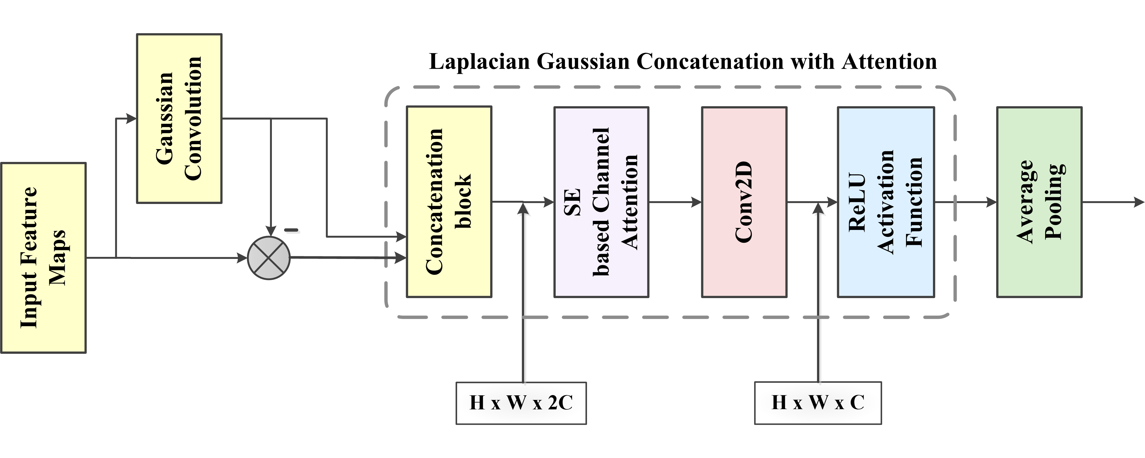
Figure 1: Laplacian Gaussian concatenation with attention pooling.

II-B The Squeeze and Excitation Network

A crucial part of the LGCA pooling technique is the channel attention block which performs the squeeze and excitation (SE) function. The SE network [42] re-weights each channel appropriately, making it more sensitive to significant features while discarding irrelevant elements. It performs three operations on the input image squeezing, excitation, and scaling. Figure 2 shows the architecture of the SE network.

Consider an image with dimension $H\times W\times C_{in}$, where the height and width of the image are represented by $H$, $W$, respectively, and $C_{in}$ represents the original number of channels. After a simple convolution operation, a feature map of size $H\times W\times C$ with different numbers of channels $C$ is extracted from the input. To extract the global information from each channel of the feature map, the squeeze operation is performed. This is achieved by implementing global average pooling (GAP) on the feature map to reduce the spatial dimension from $H\times W\times C$ to $1\times 1\times C$.

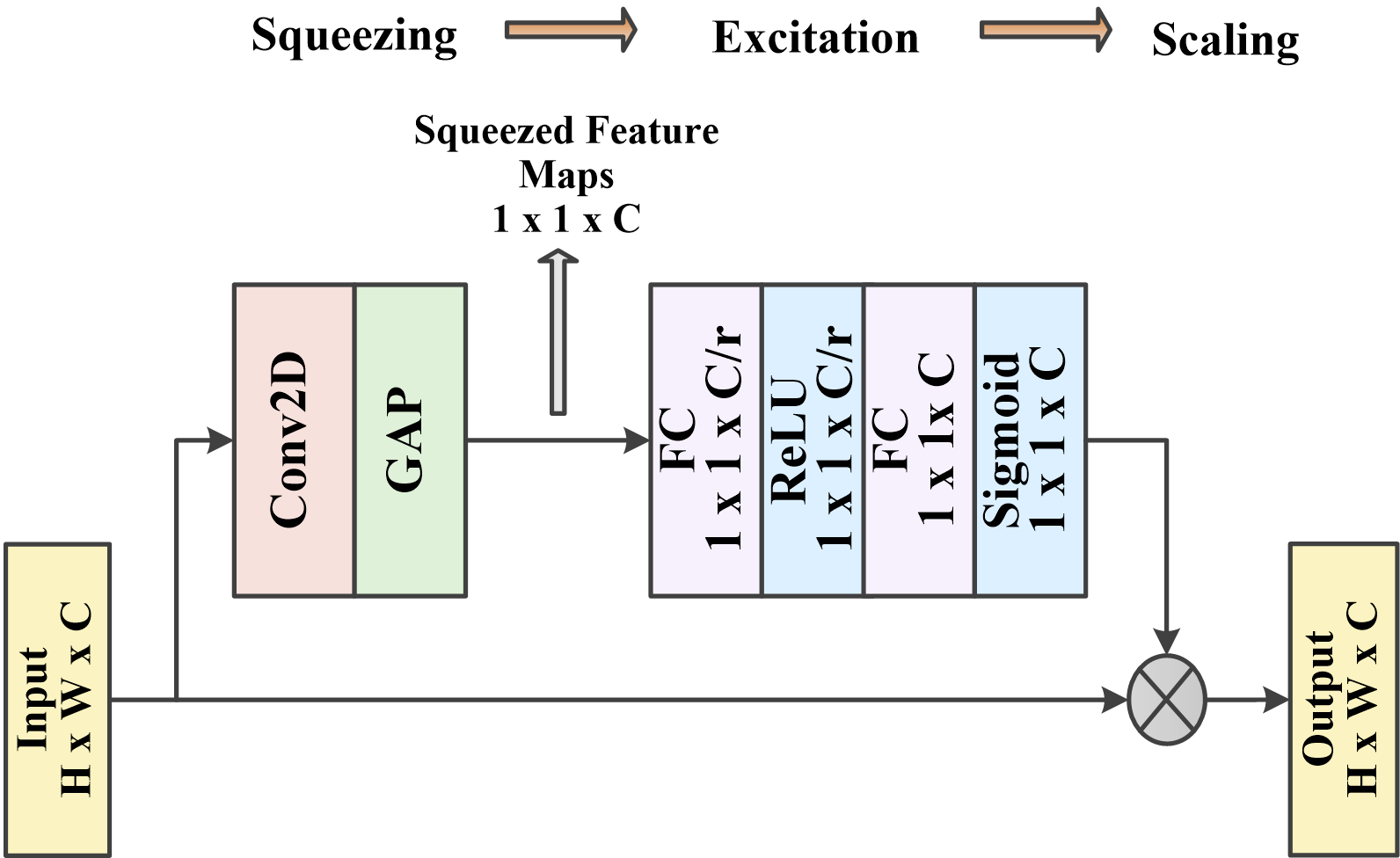
Figure 2: The squeeze and excitation function.

The excitation operation is performed on these single descriptors for each channel. Two fully connected layers with a bottleneck architecture surrounding the non-linear ReLU activation function are utilized for the excitation operation. This serves to determine the per-channel weights, which are used to adaptively re-scale the input feature map. In this bottleneck architecture, the input dimensionality-reduction layer reduces the number of channels by a factor $r=16$, which is later restored to the original number by the output dimensionality-increasing layer. The sigmoid activation function is used for estimating per-channel attention weights for each squeezed embedding. A scaling operation is performed by applying an element-wise multiplication between the output of sigmoid activation function and the input feature map. The sigmoid activation function assigns the values from $0$ to $1$ to the squeezed embedding, which helps in providing weights and generating channels with appropriate importance.

III Proposed Method

This section discusses in detail the network architecture of the LGCA attention-pooled CAE and the framework of the proposed fusion method.

III-A The Network Architecture

The network architecture of the LGCA attention-pooled CAE is shown in Figure 3. The proposed training model embodies a convolutional autoencoder DL architecture. The input is an image of dimension $256\times 256$, which is passed through an encoder and the reconstruction of this image is obtained at the output of decoder. The encoder block consists of three convolutional layers and three LGCA pooling layers comprised in an alternate manner. The convolution layer is a 2-D convolution, where a kernel of fixed size $3\times 3$ slides over the 2-D input data with stride = 1, executing element-wise multiplication and summing the result into a single output pixel. It performs the task of extensive feature extraction. The LGCA pooling serves in preserving both the low and high-frequency characteristics of the extracted feature maps. The pooling layers also execute dimensionality reduction from spatial size $256\times 256$ to the final output of the encoder with dimension $32\times 32$. Three transposed convolution layers, which perform deconvolution of the encoded input, are included in the decoder block to obtain the reconstructed image. A transposed convolutional layer aims to reconstruct the spatial dimensions of the convolutional layer and reverses the down-sampling techniques applied to it. The kernel size for these layers is fixed to $2\times 2$ with stride = 2. A $tanh$ activation function is used at the last stage of the decoder. This completes the training model architecture of the proposed method. This model is trained on a medical dataset containing numerous neurological images. The trained model is utilized for the execution of multimodal medical image fusion. TABLE I summarizes the number of input and output channels of the convolutional layers used in encoder and decoder blocks shown in Figure 3.

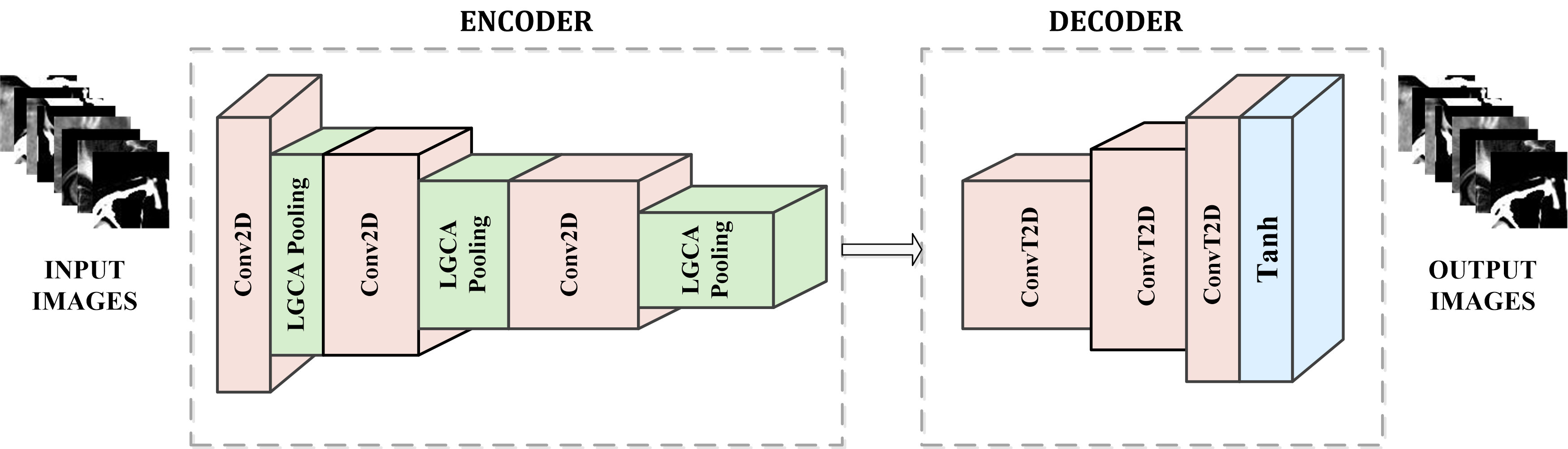
Figure 3: Network architecture of the LGCA pooled CAE used in the proposed fusion method

TABLE I: Channel details for the proposed training model

Model	Layer	Input Channel	Output Channel
Encoder	Conv2D (1)	1	64
	Conv2D (2)	64	128
	Conv2D (3)	128	256
Decoder	ConvT2D (1)	256	128
	ConvT2D (2)	128	64
	ConvT2D (3)	64	1

III-B Proposed Fusion Framework

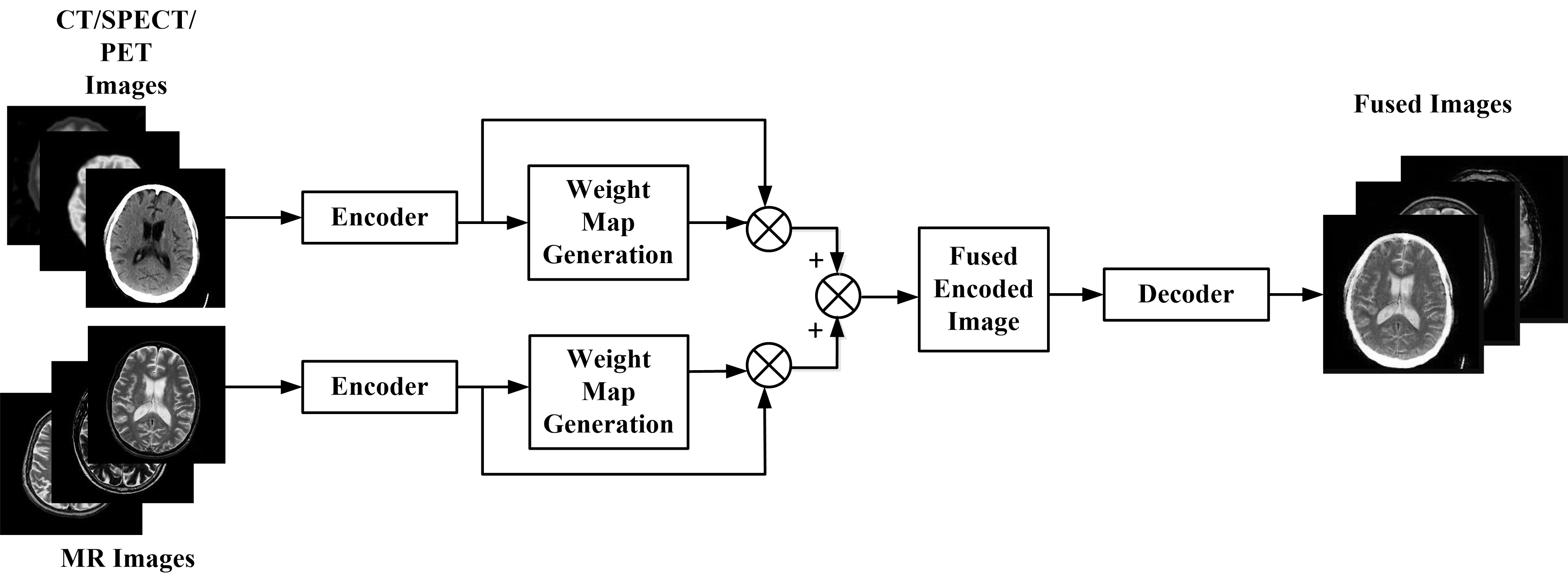
Figure 4: Image fusion framework using the trained model.

The framework for the proposed fusion method is shown in Figure 4. The trained CAE model discussed in the previous section III-A is utilized for the fusion of multimodal medical images. The two source images are passed through the encoder of the trained model and their encoded feature maps are obtained. Weight maps are obtained using a weight map generation block that captures the feature sparsity of each of the encoded feature maps. The generated weights are applied to the individual encoded source images. Next, a summation of the two weighted-encoded inputs is performed, and the encoded fused image is obtained. The encoded version of the fused image is then passed through the decoder which reconstructs the final fused image.

The implementation steps of the fusion strategy are as follows:

Step 1: Consider a pair of pre-registered CT/SPECT/PET and MR images represented as $P=P_{i,j}$ and $Q=Q_{i,j}$, respectively, where $i$ and $j$ represent the row and column indices. For color images (SPECT/PET), first, convert the images from RGB to YUV color space using the following equation;

$$\begin{bmatrix}Y_{c}\\ U_{c}\\ V_{c}\\ \end{bmatrix}=\begin{bmatrix}0.299&0.587&0.114\\ $- 0.169 $&$- 0.331$&0.5\\ 0.5&$- 0.419$&$- 0.081$\\ \end{bmatrix}\begin{bmatrix}R_{c}\\ G_{c}\\ B_{c}\\ \end{bmatrix}$$ (2)

Where, $R_{c}$, $G_{c}$, and $B_{c}$ refer to the red, green, and blue color channels of an image and $Y_{c}$, $U_{c}$, and $V_{c}$, represent the one luminance and two chrominance components, respectively. Now, consider the luminance component $Y_{c}$ for further processing.

Step 2: Subject the source images, $P_{i,j}$ and $Q_{i,j}$ to the encoder ($E$) of the trained CAE model and get encoded features $E^{P}$ and $E^{Q}$ as follows;

$$E^{P}=E(P_{i,j})$$ (3)

$$E^{Q}=E(Q_{i,j})$$ (4)

Step 3: In order to retain only the sparse features, an activity map $AM_{ij}$ is generated using $l_{1}$-norm of the encoded features $E^{P}$ and $E^{Q}$ as follows;

$$AM^{P}_{ij}=\begin{Vmatrix}E^{P}\end{Vmatrix}_{1}$$ (5)

$$AM^{Q}_{ij}=\begin{Vmatrix}E^{Q}\end{Vmatrix}_{1}$$ (6)

Step 4: A final activity map $FAM_{ij}$ is generated for each $AM_{ij}$ by performing block based averaging within a window of $3\times 3$ to improve the robustness towards misregistration. Next, the weight maps are generated as follows;

$$W^{P}_{ij}=\frac{FAM^{P}_{ij}}{FAM^{P}_{ij}+FAM^{Q}_{ij}}$$ (7)

$$W^{Q}_{ij}=\frac{FAM^{Q}_{ij}}{FAM^{P}_{ij}+FAM^{Q}_{ij}}$$ (8)

Step 5: The encoded fused image $E^{F}_{ij}$ is acquired by adding the encoded features of the two input images after convolution with the individual weight maps as follows;

$$E^{F}_{ij}=W^{P}_{ij}*E^{P}+W^{Q}_{ij}*E^{Q}$$ (9)

Step 6: Finally, generate the fused image $F=F_{i,j}$ by passing the fused encoded image to the decoder ($D$) of the trained CAE model.

$$F=D(E^{F}_{ij})$$ (10)

In the case of the color images (SPECT/PET), the color fused image is generated by performing color space conversion from YUV to RGB using the fused image $F$ and $U_{c}$, $V_{c}$ channels of the original input color images. The color space conversion is performed by using the following equation:

$$\begin{bmatrix}R_{c}\\ G_{c}\\ B_{c}\\ \end{bmatrix}=\begin{bmatrix}1&0&1.14\\ 1&$- 0.39$&0.58\\ 1&2.03&0\\ \end{bmatrix}\begin{bmatrix}F\\ U_{c}\\ V_{c}\\ \end{bmatrix}$$ (11)

IV Experimental Details

IV-A Dataset

The proposed CAE model is trained and tested on a dataset of a total of 2211 images from the Harvard Medical School’s whole brain atlas, consisting of CT-MR T2, SPECT-MR T2, and PET-MR T2 pairs, which are considered to generate the training dataset [43]. The dataset is created by dividing each original image of spatial size $256\times 256$ into four image patches of size $64\times 64$. Some patches having no or less information were discarded, and the dataset with 6756 image patches was used to train the model. The test dataset containing 100 image pairs of MR-CT, MR-SPECT, and MR-PET scans of patients with diverse neurological afflictions is used to validate the capability of the proposed method for the fusion of a range of medical images with multiple imaging modalities.

IV-B Parameter Settings and Implementation Details

The proposed model is trained for epochs = 30, batch size = 32, and learning rate $=1\times 10^{-3}$ using an Adam[44] optimizer. All these hyperparameters are set empirically. The loss function used is the mean square error (MSE) between the input image and the reconstructed image. The implementation was performed in the PyTorch framework, using the hardware platform with Intel Core Xeon(R) Silver 4210R CPU, 2.4 GHz, 128 GB RAM, and 24 GB NVIDIA GPU with Ubuntu 22.04 LTS 64-bit operating system.

A detailed comparative study between the subjective and quantitative results of the proposed and existing state-of-the-art (SOTA) fusion methods is performed to evaluate the effectiveness of the proposed fusion method. The SOTA fusion methods considered are dual-discriminator conditional GANs-based methods by Ma et al. (DDcGAN)[28], dual-stream attention mechanism based method by Fu et al. (DSAGAN)[29], a squeeze-decompose network based method by Zhang et al. (SDNet)[30], a dense net based unified fusion framework by Xu et al. (U2Fusion)[31]. Nine SOTA fusion metrics are used for quantitative evaluation as listed below,

1. Entropy ($EN$) [45]

2. Standard Deviation ($SD$) [45]

3. Spatial Frequency ($SF$) [45]

4. Edge Preservation Index ($Q_{AB/F}$) [46]

5. Mutual Information ($MI$) [47]

6. Cvejic’s metric ($Q_{C}$)[48]

7. Yang’s metric ($Q_{Y}$)[49]

8. Sum of the Correlations of Differences ($SCD$) [50]

9. Visual Information Fidelity for Fusion ($VIFF$) [51].

V Results and Discussions

V-A Visual Performance Analysis

Figure 5 provides the visual comparison of the results obtained with SOTA fusion methods and the proposed method. Figure 5 (a) and (b) shows the source MR and CT/SPECT/PET images, respectively. Fusion results of the SOTA methods and the proposed method are shown in (c)-(g). From Figure 5(g), it can be seen that the fused images obtained by the proposed fusion method have strong contrast and provide good visualization of information present in both grey and color source images. In Figure 5, zoomed regions are also highlighted by red and green squares for better visualization of the fusion results.

The fused images obtained by the DDcGAN[28] method are shown in Figure 5(c). For MR T2-CT pairs 1 and 2, the DDcGAN[28] fails to conserve the structural information in the source images with appropriate contrast. The loss of vital diagnostic edge information is also observed in the fusion results. As compared to the proposed approach, it fails to adequately preserve the soft tissue demarcation present in the MR T2 source images. The fusion results of DSAGAN[29] are shown in Figure 5(d). For grey image pairs 1 and 2, the soft tissue structure in MR T2 images is sufficiently preserved, but compared to the proposed method, the fusion results cease to preserve the significant demarcation of the skull boundaries present in CT images. For image pairs 3-6, the color information is adequately retained in the fused images, but the contrast of tissue composition in MR T2 images is not retained well. In the case of fusion methods SDNet[30] and U2Fusion[31], for MR T2-CT image pairs 1 and 2, the fusion results capture the demarcation of tissue structure in MR T2 images but fail to produce the contrast of the hard tissue composition in CT images. In the case of MR T2-SPECT/PET image pairs 3-6, both SDNet[30] and U2Fusion[31] methods lack color consistency as compared to the proposed method and the bright pixels look much darker as compared to the original MR T2 images.

Compared to the SOTA fusion methods, the visual differences in the results of the proposed fusion method are very prominent, as it proficiently highlights the global as well as local contrast of the six input image pairs. For MR T2-CT pairs 1 and 2, the fused images obtained with the proposed method provide better delineation of both soft and hard tissue structure compared to the SOTA methods. The fused images obtained with the proposed method effectively preserve the complementary information present in the source images and provide rich color consistency for multimodal color image pairs 3-6. In the fused outcomes of the proposed method in Figure 5(g), the edges are also clearly visible along with the structural and textural composition of the source images. The proposed approach provides better visualization of the source images in the fusion results, which may assist medical professionals in making an accurate clinical diagnosis in an efficient manner. Overall, from the experimental visual results, the proposed method outperforms the SOTA methods in terms of the amount of local and global feature details transferred from the source images to the fused image.

V-B Quantitative Performance Analysis

The quantitative results for image pairs in Figure 5 are presented in TABLE II. For every image pair in TABLE II, the bold text highlights the best-performing method, while underlined values represent the second-best method. The proposed method shows a significant increment for $EN$ metric for grey-scale and color multimodal image fusion which shows the amount of information present in the fusion results of the proposed approach significantly higher than in the aforementioned SOTA fusion methods. The $SD$ metric, which measures the quality of contrast of fused images compared to the individual source images, is higher for the proposed method. This implies that the fusion outcomes of the proposed method provide stronger contrast compared to other methods. The mutual information content present in fused images is measured by the $MI$ metric. The proposed approach attains the highest values for $MI$ values for most of the image pairs. The proposed method generates fusion results with minimum artifacts and distortion as compared to the other methods as higher values are observed for the visual fidelity $VIFF$ metric for most image pairs. The proposed method performs second best for the $Q_{Y}$ metric, which measures the amount of complementary information preserved. In the case of performance metrics such as $SCD$, $Q_{C}$ and $Q_{AB/F}$, SDNet[30] attains higher values for color image pairs 3-6. But the proposed method achieves better results for grey-scale image pairs 1 and 2. Despite the higher objective values gained by SDNet[30], the subjective results obtained by it are secondary to the results of the proposed method. In comparison, the proposed method accurately emulates the contrast of the source images, which is also validated by the higher values of the standard deviation $SD$ metric. Especially for the fusion of MR-CT images, the quantitative and the subjective assessments display significant appeal for the fusion results obtained with the proposed method.

Figure 5: Subjective Comparison of fusion results for State-of-the-art (SOTA) and proposed fusion method. (a) Input Image 1 (MR T2 Image), (b) Input Image 2 (CT/SPECT/PET Image), (c) DDcGAN [28], (d) DSAGAN [29], (e) SDNet [30], (f) U2Fusion [31], (g) Proposed fusion method

TABLE II: Quantitative performance of fusion methods for Figure 5

Image Pair	Fusion Methods	EN	SD	SF	$Q_{AB/F}$	MI	$Q_{C}$	$Q_{Y}$	SCD	VIFF
Pair 1	DDcGAN [28]	5.259	88.883	8.441	0.27	2.663	0.519	0.438	1.39	0.33
	DSAGAN [29]	5.373	57.505	7.989	0.348	2.779	0.606	0.587	1.082	0.25
	SDNet [30]	4.753	69.905	6.976	0.399	3.156	0.577	0.58	1.391	0.376
	U2Fusion [31]	4.623	66.876	7.156	0.52	2.996	0.625	0.661	1.359	0.441
	Proposed Method	5.881	90.002	6.466	0.405	3.267	0.582	0.609	1.459	0.56
Pair 2	DDcGAN [28]	5.21	89.66	8.048	0.255	2.756	0.491	0.365	1.457	0.277
	DSAGAN [29]	5.372	58.079	7.925	0.361	2.954	0.63	0.576	1.356	0.199
	SDNet [30]	4.65	53.994	7.062	0.334	3.077	0.6	0.55	1.409	0.221
	U2Fusion [31]	4.588	53.006	6.815	0.393	3.067	0.564	0.568	1.32	0.302
	Proposed Method	5.843	81.92	6.519	0.4	3.367	0.551	0.592	1.515	0.435
Pair 3	DDcGAN [28]	6.254	57.921	8.278	0.418	2.821	0.607	0.536	0.788	0.212
	DSAGAN [29]	5.475	71.827	8.842	0.548	3.105	0.75	0.744	1.271	0.421
	SDNet [30]	5.396	73.22	9.37	0.64	3.166	0.814	0.832	1.381	0.44
	U2Fusion [31]	5.733	73.221	8.494	0.609	3.333	0.661	0.634	0.713	0.486
	Proposed Method	6.292	83.962	8.553	0.51	3.471	0.693	0.644	0.919	0.486
Pair 4	DDcGAN [28]	6.009	55.736	8.195	0.479	2.675	0.62	0.589	0.893	0.278
	DSAGAN [29]	5.444	69.396	8.654	0.586	2.903	0.788	0.794	1.573	0.527
	SDNet [30]	5.337	68.964	9.055	0.651	3.014	0.819	0.841	1.595	0.531
	U2Fusion [31]	5.568	63.574	7.956	0.521	3.107	0.63	0.624	0.977	0.528
	Proposed Method	6.157	71.092	8.245	0.524	3.132	0.694	0.667	0.826	0.478
Pair 5	DDcGAN [28]	4.917	51.242	7.215	0.456	2.106	0.602	0.544	1.504	0.292
	DSAGAN [29]	5.33	60.022	7.424	0.564	2.408	0.692	0.652	1.82	0.517
	SDNet [30]	4.02	48.495	6.688	0.608	2.669	0.777	0.772	1.81	0.341
	U2Fusion [31]	4.29	41.843	5.917	0.47	2.512	0.618	0.548	1.693	0.343
	Proposed Method	4.997	54.125	6.532	0.501	2.444	0.703	0.674	1.678	0.393
Pair 6	DDcGAN [28]	3.85	56.12	6.775	0.339	2.57	0.581	0.548	0.766	0.247
	DSAGAN [29]	4.346	61.509	7.109	0.455	2.654	0.676	0.627	1.262	0.409
	SDNet [30]	3.222	61.262	7.151	0.514	2.784	0.746	0.736	1.568	0.474
	U2Fusion [31]	3.409	56.527	6.129	0.477	2.801	0.647	0.607	1.363	0.44
	Proposed Method	4.185	61.627	6.557	0.404	2.688	0.679	0.651	1.358	0.444

TABLE III: Averaged performance analysis for SOTA fusion methods ($\mbox{average}\pm\mbox{standard deviation}$)

Fusion Method	$EN$	$SD$	$SF$	$Q_{AB/F}$	MI	$Q_{C}$	$Q_{Y}$	$SCD$	$VIFF$
DDcGAN [28]	5.395 $\pm$ 0.627	74.144 $\pm$ 3.696	7.805 $\pm$ 0.506	0.372 $\pm$ 0.055	2.734 $\pm$ 0.220	0.551 $\pm$ 0.035	0.494 $\pm$ 0.045	1.275 $\pm$ 0.219	0.266 $\pm$ 0.042
DSAGAN [29]	5.410 $\pm$ 0.379	60.954 $\pm$ 2.898	7.900 $\pm$ 0.525	0.450 $\pm$ 0.044	2.845 $\pm$ 0.256	0.658 $\pm$ 0.049	0.633 $\pm$ 0.057	1.303 $\pm$ 0.188	0.333 $\pm$ 0.073
SDNet [30]	4.682 $\pm$ 0.529	61.700 $\pm$ 6.345	7.448 $\pm$ 0.680	0.496 $\pm$ 0.044	3.052 $\pm$ 0.247	0.690 $\pm$ 0.037	0.693 $\pm$ 0.044	1.484 $\pm$ 0.117	0.370 $\pm$ 0.079
U2Fusion [31]	4.744 $\pm$ 0.546	56.867 $\pm$ 6.788	6.97 $\pm$ 0.569	0.467 $\pm$ 0.046	2.973 $\pm$ 0.258	0.586 $\pm$ 0.051	0.592 $\pm$ 0.056	1.274 $\pm$ 0.222	0.393 $\pm$ 0.076
Proposed Method	5.696 $\pm$ 0.487	71.314 $\pm$ 6.513	6.786 $\pm$ 0.642	0.499 $\pm$ 0.046	3.064 $\pm$ 0.303	0.596 $\pm$ 0.059	0.592 $\pm$ 0.050	1.387 $\pm$ 0.228	0.409 $\pm$ 0.078

To present a more concise analysis of the aforementioned fusion methods, the averaged quantitative performance is presented in TABLE III and the following observations are drawn,

1. The proposed method achieves 5.58%, 5.29%, 21.66% and 20.07% greater values of $EN$ than the methods mentioned in TABLE II DDcGAN[28], DSAGAN[29], SDNet[30] and U2Fusion[31], respectively. The greater entropy values show that, in comparison to other approaches, the proposed method’s fusion outcomes have rich information content, which validates the visual performance analysis.

2. In comparison to the methods DDcGAN[28], DSAGAN[29], SDNet[30] and U2Fusion[31], for $MI$ metric, the proposed method provides 12.07%, 7.7%, 0.39% and 3.06% higher values, respectively. The fusion outcomes of the proposed approach are improved by the overall higher extent of aggregated information captured from the source images.

3. The proposed method yields 53.76%, 22.82%, 10.54% and 4.07% higher values of $VIFF$ than the aforementioned methods DDcGAN[28], DSAGAN[29], SDNet[30] and U2Fusion[31], respectively. It implies that the proposed approach surpasses other fusion methods for the visual fidelity index and provides fusion results that are visually consistent, without distortion and artifacts.

4. For $SD$ measure, the proposed method attains 17%, 15.58%, and 25.4% higher values for the methods DSAGAN[29], SDNet[30] and U2Fusion[31], respectively which denotes that the proposed method’s fusion outcomes have superior contrast than the earlier mentioned methods.

5. The proposed method gets 2.51%, 0.31%, and 2.59% greater values of $SCD$ than the methods DDcGAN[28], DSAGAN[29] and U2Fusion[31], respectively. This implies that the proposed method’s fusion outcomes have a higher correlation with the reference images and the complementary information is also well-preserved.

V-C Ablation Studies:

To explore the effectiveness of the LGCA pooling technique in enhancing the capability of the proposed fusion approach, an ablation study is conducted with the two most common techniques i.e. average and max pooling. The visual comparison is presented in Figure 6. Here, Figure 6 (a) and (b) display the source images and Figure 6 (c), (d), and (e) display the fusion results obtained by employing the average, max, and LGCA pooling techniques, respectively, in the CAE architecture used in the proposed fusion method. The rest of the blocks of the CAE, dataset, hyperparameters, and implementation platform are kept the same. Figure 6 shows specific zoomed regions of the fused images for better visualization of the results obtained using each pooling technique.

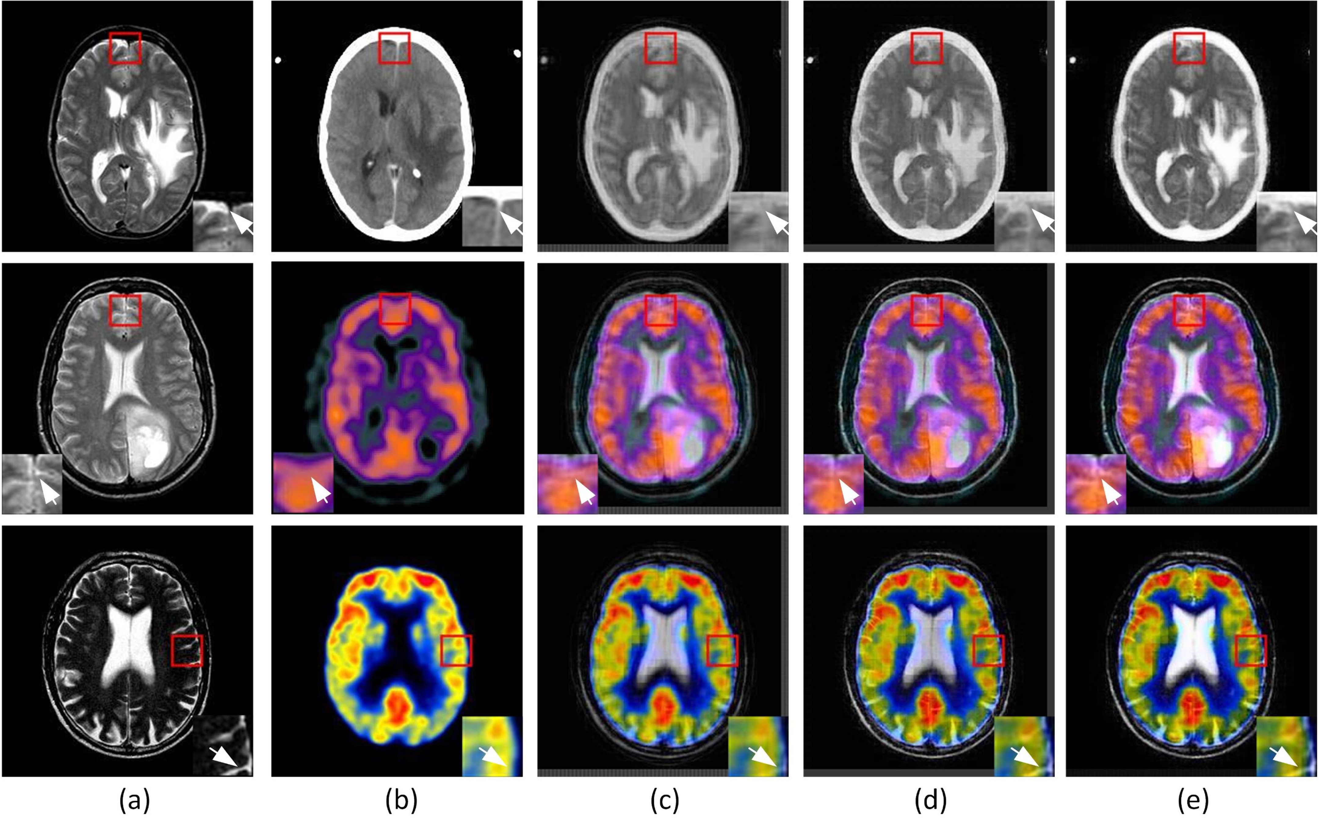
Figure 6: Subjective Comparison of fusion results with three pooling methods (a) Input Image 1 (MR T2 Image), (b) Input Image 2 (CT/SPECT/PET Image), (c) Average pooling, (d) Max pooling, (e) LGCA pooling.

It can be observed from Figure 6 that the fusion results of each pooling technique capture the structural information accurately but for the average pooling in Figure 6 (c), the fused images are of very low resolution with muted edges and blurred spatial details of the input images. Efficient preservation of the edge information with vivid contrast is observed in the fusion results of the LGCA pooling. For MR T2-CT fusion, compared to the max pool fused image, both soft and hard tissue demarcations with strong contrast are produced in the fusion result of LGCA pooling. For MR T2-SPECT and MR T2-PET fusion, compared to the max pool, LGCA pooling fusion results are of richer color consistency and finer local as well as global contrast. The soft tissue delineation along the skull’s inner boundary in MR images is also more prominent in the resultant fused images with the LGCA pooling method. Compared to the fusion results of the other pooling techniques, the complementary information is preserved to a greater extent by the LGCA pooling.

TABLE IV: Quantitative performance of the pooling methods for Figure 6

Image Pair	Pooling Methods	EN	SD	SF	$Q_{AB/F}$	MI	$Q_{C}$	$Q_{Y}$	SCD	VIFF
Pair 1	Average	5.808	65.671	6.034	0.247	3.177	0.511	0.489	1.220	0.362
	Max	6.015	71.339	5.783	0.371	3.447	0.558	0.586	1.319	0.429
	LGCA	5.882	78.805	6.186	0.420	3.436	0.589	0.630	1.464	0.448
Pair 2	Average	6.163	66.467	6.670	0.222	3.034	0.530	0.488	0.637	0.443
	Max	6.130	66.789	6.795	0.407	3.267	0.617	0.600	0.650	0.503
	LGCA	5.997	70.970	6.883	0.468	3.373	0.681	0.669	0.871	0.501
Pair 3	Average	5.434	65.347	7.079	0.220	2.653	0.457	0.526	1.511	0.308
	Max	5.436	64.780	7.183	0.329	2.837	0.526	0.587	1.580	0.346
	LGCA	5.339	68.585	7.154	0.350	2.927	0.554	0.598	1.681	0.338

TABLE V: Averaged subjective performance analysis for pooling methods ($\mbox{average}\pm\mbox{standard deviation}$)

Pooling Method	EN	SD	SF	$Q_{AB/F}$	MI	$Q_{C}$	$Q_{Y}$	SCD	VIFF
Average	5.780 $\pm$ 0.460	62.709 $\pm$ 5.557	6.482 $\pm$ 0.600	0.191 $\pm$ 0.022	2.763 $\pm$ 0.250	0.438 $\pm$ 0.061	0.422 $\pm$ 0.050	1.025 $\pm$ 0.251	0.344 $\pm$ 0.06
Max	5.893 $\pm$ 0.445	66.449 $\pm$ 4.935	6.558 $\pm$ 0.641	0.338 $\pm$ 0.038	3.014 $\pm$ 0.283	0.525 $\pm$ 0.047	0.535 $\pm$ 0.039	1.104 $\pm$ 0.269	0.400 $\pm$ 0.067
LGCA	5.696 $\pm$ 0.487	71.314 $\pm$ 6.513	6.786 $\pm$ 0.642	0.399 $\pm$ 0.046	3.064 $\pm$ 0.303	0.566 $\pm$ 0.059	0.592 $\pm$ 0.050	1.307 $\pm$ 0.228	0.409 $\pm$ 0.078

The quantitative performance analysis for Figure 6 is presented in TABLE IV. In TABLE IV, for each image pair, the LGCA pooling achieves the highest values for performance measures SD, $Q_{AB/F}$, $Q_{C}$, $Q_{Y}$ and SCD which further supports the visual evaluation of the fusion results. Overall for EN metric, Max-pool shows significant performance but LGCA-pooling gains notable results for MI values. Discussing the visual clarity in fusion outcomes, LGCA-pool has an overall marked increment in SF measure. The proposed fusion method achieves top performance for visual information metric VIFF, in case of CT-MR fusion, and comes in second to max-pool for the fusion of anatomical-functional pairs 2 and 3 in TABLE IV.

The averaged quantitative analysis for the three pooling techniques is presented in TABLE V. It is observed that the proposed method has significantly better results for metrics SD, SF, $Q_{AB/F}$, MI, $Q_{C}$, $Q_{Y}$ and SCD. The following observations are drawn,

1. The proposed method with LGCA pooling achieves 13.72% and 7.32% higher values of $SD$ than the average and max pooling methods, respectively which imply superior contrast as compared to the conventional pooling methods.

2. The $SF$ performance parameter measures the clarity or sharpness of the fused images. For this metric, the LGCA pooling achieves 4.69% and 3.48% greater values compared to the average and max pooling, respectively.

3. The proposed method with LGCA pooling achieves 10.89% and 1.66% higher values of MI than the average and max pooling methods, respectively which signify higher visual information.

4. The $Q_{C}$ metric measures the amount of local similarities preserved with minimum deformations between the source and fused images which exist in the same spatial position. The proposed method with LGCA pooling has 29.22% and 7.81% greater values than the average and max pool techniques, respectively.

5. For $Q_{Y}$ measure, the LGCA pooling achieves 40.28% and 10.65% higher values than the average and max pooling, respectively. This shows that, compared to other approaches, the fusion results achieved using LGCA pooling preserve the complementary information of the reference images far better.

6. In comparison to the average and max pooling, the LGCA pooling method produces $SCD$ values that are 27.51% and 18.39% greater, respectively, indicating that the source and fused images achieve higher correlation.

7. For the edge preservation index $Q_{AB/F}$, the proposed method with LGCA pooling yields 108.9% and 18.05% higher values than the average and max pooling, respectively which refers to the amount of edge information.

8. The LGCA pooling-based proposed model exceeds the results of average and max pooling, respectively, by 18.9% and 2.25% for the $VIFF$ metric, indicating the presence of more prominent visual information with minimum distortion and artifacts.

Based on the above observations, it can be observed that the proposed method with the LGCA pooling layer achieves notable improvement in visual and quantitative fusion results as compared to the conventional pooling layers.

VI Conclusion

This paper presents a convolutional autoencoder (CAE)-based multimodal medical image fusion method that integrates a Laplacian-Gaussian concatenation with an attention pooling technique as a viable substitute for the conventional pooling methods. The LGCA pooling layers used in the encoder block help in retaining both the high and low-frequency features of the source images leading to the effective preservation of tissue contrast and edges. The weighted average fusion strategy combines the encoded feature maps of the two inputs and helps in the effective reconstruction of the resultant fused image using the trained decoder. Furthermore, training the fusion model on neurological images helps to capture the inherent characteristics of a variety of brain tissues and improves the visualization of the fused images. Detailed performance analysis demonstrates that the proposed fusion method provides fused images with improved visual quality and also outperforms the existing fusion methods in quantitative assessment.

References

- [1] S. Li, X. Kang, L. Fang, J. Hu, and H. Yin, “Pixel-level image fusion: A survey of the state of the art,” information Fusion, vol. 33, pp. 100–112, 2017.
- [2] S. Singh and R. S. Anand, “Multimodal medical image sensor fusion model using sparse k-svd dictionary learning in nonsubsampled shearlet domain,” IEEE transactions on instrumentation and measurement, vol. 69, no. 2, pp. 593–607, 2019.
- [3] M. Das, D. Gupta, P. Radeva, and A. M. Bakde, “Optimized multimodal neurological image fusion based on low-rank texture prior decomposition and super-pixel segmentation,” IEEE Transactions on Instrumentation and Measurement, pp. 1–9, 2022.
- [4] J. Du, W. Li, K. Lu, and B. Xiao, “An overview of multi-modal medical image fusion,” Neurocomputing, vol. 215, pp. 3–20, 2016.
- [5] S. Singh and D. Gupta, “Detail enhanced feature-level medical image fusion in decorrelating decomposition domain,” IEEE Transactions on Instrumentation and Measurement, vol. 70, pp. 1–9, 2021.
- [6] H. Hermessi, O. Mourali, and E. Zagrouba, “Multimodal medical image fusion review: Theoretical background and recent advances,” Signal Processing, vol. 183, p. 108036, 2021.
- [7] J. Du, W. Li, and H. Tan, “Intrinsic image decomposition-based grey and pseudo-color medical image fusion,” IEEE Access, vol. 7, pp. 56443–56456, 2019.
- [8] S. Singh and R. Anand, “Multimodal medical image fusion using hybrid layer decomposition with cnn-based feature mapping and structural clustering,” IEEE Transactions on Instrumentation and Measurement, vol. 69, no. 6, pp. 3855–3865, 2020.
- [9] X. Liu, W. Mei, and H. Du, “Multi-modality medical image fusion based on image decomposition framework and nonsubsampled shearlet transform,” Biomedical Signal Processing and Control, vol. 40, pp. 343–350, 2018.
- [10] X. Li, X. Guo, P. Han, X. Wang, H. Li, and T. Luo, “Laplacian redecomposition for multimodal medical image fusion,” IEEE Transactions on Instrumentation and Measurement, vol. 69, no. 9, pp. 6880–6890, 2020.
- [11] M. Yin, X. Liu, Y. Liu, and X. Chen, “Medical image fusion with parameter-adaptive pulse coupled neural network in nonsubsampled shearlet transform domain,” IEEE Transactions on Instrumentation and Measurement, vol. 68, no. 1, pp. 49–64, 2018.
- [12] J.-j. Zong and T.-s. Qiu, “Medical image fusion based on sparse representation of classified image patches,” Biomedical Signal Processing and Control, vol. 34, pp. 195–205, 2017.
- [13] Z. Wang, Z. Cui, and Y. Zhu, “Multi-modal medical image fusion by laplacian pyramid and adaptive sparse representation,” Computers in Biology and Medicine, vol. 123, p. 103823, 2020.
- [14] Y. Yang, Y. Que, S. Huang, and P. Lin, “Multimodal sensor medical image fusion based on type-2 fuzzy logic in nsct domain,” IEEE Sensors Journal, vol. 16, no. 10, pp. 3735–3745, 2016.
- [15] M. Manchanda and R. Sharma, “An improved multimodal medical image fusion algorithm based on fuzzy transform,” Journal of Visual Communication and Image Representation, vol. 51, pp. 76–94, 2018.
- [16] N. Padmavathi and others, “Fusion of multimodal abdominal cancerous images and classification using support vector machine,” in 2017 International Conference on Intelligent Sustainable Systems (ICISS), pp. 266–269, IEEE, 2017.
- [17] N. Zhang, Q. Liao, S. Ruan, S. Lebonvallet, and Y. Zhu, “Multi-kernel SVM based classification for tumor segmentation by fusion of MRI images,” in 2009 IEEE International Workshop on Imaging Systems and Techniques, pp. 71–75, IEEE, 2009.
- [18] H. Kaur, D. Koundal, and V. Kadyan, “Image fusion techniques: a survey,” Archives of computational methods in Engineering, vol. 28, pp. 4425–4447, 2021.
- [19] L. Cai, J. Gao, and D. Zhao, “A review of the application of deep learning in medical image classification and segmentation,” Annals of translational medicine, vol. 8, no. 11, 2020.
- [20] Y. Liu, X. Chen, Z. Wang, Z. J. Wang, R. K. Ward, and X. Wang, “Deep learning for pixel-level image fusion: Recent advances and future prospects,” Information Fusion, vol. 42, pp. 158–173, 2018.
- [21] Y. Liu, X. Chen, R. K. Ward, and Z. J. Wang, “Medical image fusion via convolutional sparsity based morphological component analysis,” IEEE Signal Processing Letters, vol. 26, no. 3, pp. 485–489, 2019.
- [22] F. Liu, L. Chen, L. Lu, A. Ahmad, G. Jeon, and X. Yang, “Medical image fusion method by using laplacian pyramid and convolutional sparse representation,” Concurrency and Computation: Practice and Experience, vol. 32, no. 17, p. e5632, 2020.
- [23] P.-F. Wang, X.-Q. Luo, X.-Y. Li, and Z.-C. Zhang, “Image fusion based on shift invariant shearlet transform and stacked sparse autoencoder,” Journal of Algorithms & Computational Technology, vol. 12, no. 2, pp. 73–84, 2018.
- [24] N. Tawfik, H. A. Elnemr, M. Fakhr, M. I. Dessouky, and F. E. A. El-Samie, “Multimodal medical image fusion using stacked auto-encoder in nsct domain,” Journal of Digital Imaging, vol. 35, no. 5, pp. 1308–1325, 2022.
- [25] K. Wang, M. Zheng, H. Wei, G. Qi, and Y. Li, “Multi-modality medical image fusion using convolutional neural network and contrast pyramid,” Sensors, vol. 20, no. 8, p. 2169, 2020.
- [26] K.-j. Xia, H.-s. Yin, and J.-q. Wang, “A novel improved deep convolutional neural network model for medical image fusion,” Cluster Computing, vol. 22, pp. 1515–1527, 2019.
- [27] H. Zhang, H. Xu, X. Tian, J. Jiang, and J. Ma, “Image fusion meets deep learning: A survey and perspective,” Information Fusion, vol. 76, pp. 323–336, 2021.
- [28] J. Ma, H. Xu, J. Jiang, X. Mei, and X.-P. Zhang, “DDcGAN: A dual-discriminator conditional generative adversarial network for multi-resolution image fusion,” IEEE Transactions on Image Processing, vol. 29, pp. 4980–4995, 2020.
- [29] J. Fu, W. Li, J. Du, and L. Xu, “DSAGAN: A generative adversarial network based on dual-stream attention mechanism for anatomical and functional image fusion,” Information Sciences, vol. 576, pp. 484–506, 2021.
- [30] H. Zhang and J. Ma, “SDNet: A versatile squeeze-and-decomposition network for real-time image fusion,” International Journal of Computer Vision, vol. 129, pp. 2761–2785, 2021.
- [31] H. Xu, J. Ma, J. Jiang, X. Guo, and H. Ling, “U2Fusion: A unified unsupervised image fusion network,” IEEE Transactions on Pattern Analysis and Machine Intelligence, vol. 44, no. 1, pp. 502–518, 2020.
- [32] A. Azarang, H. E. Manoochehri, and N. Kehtarnavaz, “Convolutional autoencoder-based multispectral image fusion,” IEEE access, vol. 7, pp. 35673–35683, 2019.
- [33] J. Qu, Y. Shi, W. Xie, Y. Li, X. Wu, and Q. Du, “Mssl: Hyperspectral and panchromatic images fusion via multiresolution spatial–spectral feature learning networks,” IEEE Transactions on Geoscience and Remote Sensing, vol. 60, pp. 1–13, 2021.
- [34] Y. Zhang, “A better autoencoder for image: Convolutional autoencoder,” in ICONIP17-DCEC. Available online: http://users. cecs. anu. edu. au/Tom. Gedeon/conf/ABCs2018/paper/ABCs2018_paper_58. pdf (accessed on 23 March 2017), 2018.
- [35] J. Masci, U. Meier, D. Cireşan, and J. Schmidhuber, “Stacked convolutional auto-encoders for hierarchical feature extraction,” in Artificial Neural Networks and Machine Learning–ICANN 2011: 21st International Conference on Artificial Neural Networks, Espoo, Finland, June 14-17, 2011, Proceedings, Part I 21, pp. 52–59, Springer, 2011.
- [36] M. Chen, X. Shi, Y. Zhang, D. Wu, and M. Guizani, “Deep feature learning for medical image analysis with convolutional autoencoder neural network,” IEEE Transactions on Big Data, vol. 7, no. 4, pp. 750–758, 2017.
- [37] C. Vasconcelos, H. Larochelle, V. Dumoulin, R. Romijnders, N. Le Roux, and R. Goroshin, “Impact of aliasing on generalization in deep convolutional networks,” in Proceedings of the IEEE/CVF International Conference on Computer Vision, pp. 10529–10538, 2021.
- [38] A. H. Ribeiro and T. B. Schön, “How convolutional neural networks deal with aliasing,” in ICASSP 2021-2021 IEEE International Conference on Acoustics, Speech and Signal Processing (ICASSP), pp. 2755–2759, IEEE, 2021.
- [39] A. Azulay and Y. Weiss, “Why do deep convolutional networks generalize so poorly to small image transformations?,” arXiv preprint arXiv:1805.12177, 2018.
- [40] R. Nirthika, S. Manivannan, A. Ramanan, and R. Wang, “Pooling in convolutional neural networks for medical image analysis: a survey and an empirical study,” Neural Computing and Applications, vol. 34, no. 7, pp. 5321–5347, 2022.
- [41] A. Sineesh and M. R. Panicker, “Exploring Novel Pooling Strategies for Edge Preserved Feature Maps in Convolutional Neural Networks,” arXiv preprint arXiv:2110.08842, 2021.
- [42] J. Hu, L. Shen, and G. Sun, “Squeeze-and-excitation networks,” in Proceedings of the IEEE conference on computer vision and pattern recognition, pp. 7132–7141, 2018.
- [43] D. Summers, “Harvard whole brain atlas: www. med. harvard. edu/aanlib/home. html,” Journal of Neurology, Neurosurgery & Psychiatry, vol. 74, no. 3, pp. 288–288, 2003.
- [44] D. P. Kingma and J. Ba, “Adam: A method for stochastic optimization,” arXiv preprint arXiv:1412.6980, 2014.
- [45] M. Das, D. Gupta, P. Radeva, and A. M. Bakde, “NSST domain CT–MR neurological image fusion using optimised biologically inspired neural network,” IET Image Processing, vol. 14, no. 16, pp. 4291–4305, 2020.
- [46] C. S. Xydeas, V. Petrovic, and others, “Objective image fusion performance measure,” Electronics letters, vol. 36, no. 4, pp. 308–309, 2000.
- [47] G. Qu, D. Zhang, and P. Yan, “Information measure for performance of image fusion,” Electronics letters, vol. 38, no. 7, p. 1, 2002.
- [48] N. Cvejic, A. Loza, D. Bull, and N. Canagarajah, “A similarity metric for assessment of image fusion algorithms,” International journal of signal processing, vol. 2, no. 3, pp. 178–182, 2005.
- [49] S. Li, R. Hong, and X. Wu, “A novel similarity based quality metric for image fusion,” in 2008 International Conference on Audio, Language and Image Processing, pp. 167–172, IEEE, 2008.
- [50] V. Aslantas and E. Bendes, “A new image quality metric for image fusion: The sum of the correlations of differences,” Aeu-international Journal of electronics and communications, vol. 69, no. 12, pp. 1890–1896, 2015.
- [51] Y. Han, Y. Cai, Y. Cao, and X. Xu, “A new image fusion performance metric based on visual information fidelity,” Information fusion, vol. 14, no. 2, pp. 127–135, 2013.