Analytical calculations of the tenth order QED radiative corrections to lepton anomalies within the Mellin–Barnes representation

Abstract

We investigate the radiative quantum electrodynamic (QED) corrections to the lepton ($\displaystyle L=e,~{}\mu$ and $\displaystyle\tau$) anomalous magnetic moment due to the contributions of diagrams with insertions of the photon vacuum polarisation operator consisting solely of four closed lepton ($\displaystyle l=e,~{}\mu$ and $\displaystyle\tau$) loops. Moreover, we focus on specific operators with two loops formed by leptons $\displaystyle L$ of the same type as the external one, the other two formed by leptons $\displaystyle\ell$ different from $\displaystyle L$. The approach is essentially based on the employment of the Mellin–Barnes representation of the $\displaystyle x$-parametrization of the corresponding Feynman diagrams. This allows one to obtain, for the first time, exact analytical expressions for the radiative corrections of the tenth order w.r.t. the electromagnetic coupling constant $\displaystyle e$. Analytically, the radiative corrections are expressed in terms of the ratio $\displaystyle r=m_{\ell}/m_{L}$ of the internal to external lepton masses. The dependence on $\displaystyle r$ is investigated numerically in the whole interval of $\displaystyle r$, $\displaystyle 0<r<\infty$. To make comparisons with earlier published results possible, our exact analytical expressions are expanded about $\displaystyle r=0$ and $\displaystyle r\to\infty$ and compared with the corresponding asymptotic expansions known in the literature.

I Introduction

Among the most important consequences of the Dirac theory is the prediction dirac that the gyromagnetic factor $\displaystyle g_{L}$ of a lepton $\displaystyle L$ is $\displaystyle g_{L}=2$. However, the self-interaction with photons leads to a gyromagnetic factor $\displaystyle g_{L}\neq 2$, which in the literature is referred to as the lepton anomaly, $\displaystyle a_{L}=(g_{L}-2)/2\neq 0$. Obviously, this anomaly is an important characteristic of the magnetic field surrounding a lepton and, in spite of its extremely small deviation from zero, it can serve as a substantial test of the Standard Model (SM) or even can indicate the existence of some “new physics” beyond the SM. Clearly, the self-energy correction to the lepton electromagnetic vertex originates not only from the electromagnetic interaction but also from strong and weak interactions. A comprehensive review of contributions of different mechanisms to $\displaystyle a_{L}$ can be found in, e.g., Refs. Jegerlehner:2017gek ; review-2021 . At present, experimental measurements of $\displaystyle a_{L}$ for electrons Parker:2018vye ; Morel and muons E989 ; Fermilab2023 are performed with an extremely high accuracy which imposes appropriate requirements on theoretical calculations. First theoretical calculations of the leading order corrections were performed by J. S. Schwinger Schwinger1948 and found to be $\displaystyle a_{L}=\alpha/2\pi$, where $\displaystyle\alpha$ is the fine structure constant. Next to the leading order corrections involve much more diagrams which result in complicate and cumbersome calculations Petermann:1957hs ; Sommerfield:1957zz . Usually, high precision numerical calculations of the radiative corrections are performed numerically by expressing a full set of Feynman diagrams via a number of master integrals associated to all possible, at a given order, topologies with a subsequent analytical fit by the known PSLQ algorithm PSLQ1992 . So the full set of the eighth order corrections contains more than 890 diagrams, which can be expressed by means of 334 master integrals belonging to 220 topologies. Then applying the PSLQ algorithm to the master integrals, one achieves a very high precision (more than 1100 digits) for the corresponding corrections, cf. Refs. Laporta:2017okg ; elliptic1 . However, such numerical calculations are rather computer resources consuming and, in addition, detailed investigations of the role of different mechanisms contributing to $\displaystyle a_{L}$ are hindered. Therefore, it is enticing to find at least a subset of specific Feynman diagrams which can provide analytical expressions even if only for a restricted number of perturbative terms. Then, having at hand analytical expressions, one can perform calculations with any desired accuracy and, consequently, use as excellent tests of the reliability of direct numerical procedures. In addition, a detailed analysis of the contribution of different lepton loops to $\displaystyle a_{L}$ will become a possible. It turns out that the subset of diagrams with loops originating only from insertions of the photon polarisation operator, the so-called “bubble”-like diagrams, allows for analytical calculations of corrections up to fairly high orders. The distinctive peculiarity of this subset is that each diagram with an arbitrary number of inserted loops can be expressed via one diagram of the second order with the exchange of only one but massive photon. The explicit expression for these kinds of massive diagrams is well known in the literature berestetski ; brodski and its analytical form permits further mathematical manipulations to obtain final analytical formulae for each considered diagram. The main idea is to apply the dispersion relations to the corresponding Feynman diagram to express it via the Feynman $\displaystyle x$-parametrization of the second-order diagram with massive photons and finally to apply the Mellins–Barnes representation to the massive photon propagator and again the dispersion relations to the polarisation operators of the internal lepton $\displaystyle\ell\neq L$ different from the external one. In this way, one can express any diagram from the mentioned subset in a rather simple form as a comvolution integral of two Mellin momenta (for details, cf. Ref. Solovtsova23 ). Then, if possible, this integral is carried out analytically providing the desired exact expressions for $\displaystyle a_{L}$.

As the first formulations of the approach, one can mention Ref. Aguilar:2008qj , where the corrections to the muon anomaly of the eighth and tenth order were calculated in analytical form as asymptotic expansions at $\displaystyle r=m_{\ell}/m_{L}\ll 1$ and $\displaystyle r\to\infty$. Further generalisation of the method for the anomalous magnetic moment of any kind of leptons to obtain exact analytical expressions up to the eighth order for any possible combination of lepton masses, i.e. for arbitrary $\displaystyle r$ ranging in the interval $\displaystyle(0<r<\infty)$, was reported in detail in Ref. Solovtsova23 .

This paper is a necessary continuation of our previous studies Solovtsova23 of the lepton anomaly within the Mellin-Barnes representation and is dedicated to analytical investigations of the tenth order corrections from Feynman diagrams with insertions of four lepton loops. Hitherto corrections of the order $\displaystyle\alpha^{5}$ have been considered either in the asymptotic limit $\displaystyle r\ll 1$ Aguilar:2008qj or only for diagrams with four lepton loops, all of the same type vesti . Below we consider another type of four loop diagrams, namely, the ones with two leptons $\displaystyle L$ of the same kind as the external one, the other two leptons $\displaystyle\ell$ different from $\displaystyle L$. The general formalism used in this paper is basically the one reported before in Refs. Aguilar:2008qj ; Solovtsova23 .

Our paper is organised as follows. In order to facilitate the reading of the paper, in Section II we briefly recall the main definitions relevant to calculations of the lepton anomaly. The general formula for QED corrections to $\displaystyle a_{L}$ from the Feynman diagrams with the insertion of an arbitrary number $\displaystyle n$ of lepton loops of two kinds is derived. The resulting convolution integral of two Mellin momenta determining the anomaly $\displaystyle a_{L}$ is presented explicitly in the most general form. The explicit expression for each Mellin momentum is derived in Section III. The details of calculations of the integral by the Cauchy theorem are discussed in Subsections III.1 and III.2 in the left ($\displaystyle r<1$) and right ($\displaystyle r>1$) semiplanes of the complex Mellin variable $\displaystyle s$, respectively. The results of numerical calculations of corrections $\displaystyle a_{L}$ for each type of leptons $\displaystyle e$, $\displaystyle\mu$ and $\displaystyle\tau$ with the insertion of loops with all possible combinations of internal leptons ($\displaystyle e$, $\displaystyle\mu$ and $\displaystyle\tau$) together with a brief discussion are presented in Section IV. In Section V, the exact analytical expressions for $\displaystyle a_{L}$ are expanded in Taylor series at $\displaystyle r\ll 1$ and $\displaystyle r\gg 1$ and compared with the corresponding asymptotic expansions known in the literature and with the numerical result of exact calculations. The conclusions and summary are presented Section VI.

II Basic formalism

In this Section, we consider the most general form of the QED corrections to the lepton anomalous magnetic moment due to bubble-like Feynman diagrams with the insertion of the photon polarization operator with an arbitrary number $\displaystyle n=p+j$ of loops, where $\displaystyle p$ is the number of loops formed by leptons $\displaystyle L$ of the same type as the external one, $\displaystyle j$ denotes the leptons $\displaystyle\ell\neq L$. The corresponding Feynman diagram is depicted in Fig. 1, left panel. It is straightforward to show Lautrup:1969fr (see also Aguilar:2008qj ; Solovtsova23 ) that the electromagnetic vertex can be related to the vertex diagram of the second order with exchanges of one but massive photon, right panel in Fig. 1. Direct calculation of the electromagnetic vertex $\displaystyle\Gamma_{\mu}(p_{1},p_{2})$ on the left diagram in Fig. 1 provides

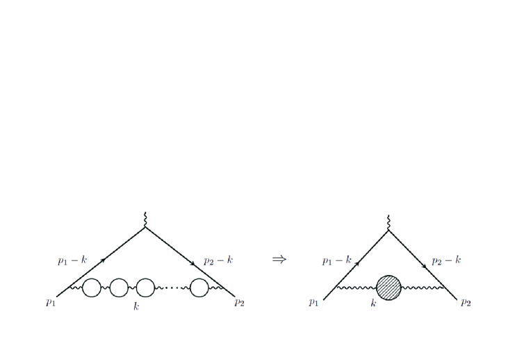
Figure 1: The Feynman diagrams considered in this paper contributing to the lepton anomalous magnetic moment. Left panel: radiative corrections to the electromagnetic lepton vertex with insertions of the vacuum polarisation operator with an arbitrary number $\displaystyle n$ of lepton loops. Right panel: the second order diagram representing the set of graphs depicted in the left panel as exchanges of one massive photon, see the text.

$$\displaystyle\Gamma_{\mu}(p_{1},p_{2})=-ie\frac{e^{2}}{(2\pi)^{4}}\int d^{4}k\gamma_{\alpha}\frac{(\hat{p_{2}}-\hat{k}+m_{L})\gamma_{\mu}(\hat{p_{1}}-\hat{k}+m_{L})}{(k^{2}-2p_{2}k)(k^{2}-2p_{1}k)}\gamma_{\alpha}\frac{\widetilde{\Pi}(k^{2})}{k^{2}}$$ (1)

$$\displaystyle=-ie\frac{e^{2}}{(2\pi)^{4}}\int\frac{dt}{t}\frac{1}{\pi}\frac{\mbox{\rm Im}\widetilde{\Pi}(t)}{k^{2}-t}\int d^{4}k\gamma_{\alpha}\frac{(\hat{p_{2}}-\hat{k}+m_{L})\gamma_{\mu}(\hat{p_{1}}-\hat{k}+m_{L})}{(k^{2}-2p_{2}k)(k^{2}-2p_{1}k)}=$$

$$\displaystyle\frac{1}{\pi}\int\frac{dt}{t}{\mbox{\rm Im}}\widetilde{\Pi}(t)\underbrace{\left[-ie\frac{e^{2}}{(2\pi)^{4}}\int d^{4}k\gamma_{\alpha}\frac{(\hat{p_{2}}-\hat{k}+m_{L})\gamma_{\mu}(\hat{p_{1}}-\hat{k}+m_{L})}{(k^{2}-2p_{2}k)(k^{2}-2p_{1}k)}\gamma_{\alpha}\frac{1}{k^{2}-t}\right]}_{\Gamma_{\mu}^{(2)}(p_{1},p_{2},t)}$$ (2)

where $\displaystyle\Gamma_{\mu}^{(2)}(p_{1},p_{2},t)$ is the lepton electromagnetic vertex for the second order diagrams with the exchange of one massive photon with mass $\displaystyle m_{\gamma}^{2}=t$, as depicted in Fig. 1, right panel.

Consequently, the anomalous magnetic moment $\displaystyle a_{L}$ is directly related to the corresponding anomalous magnetic moment induced by such a massive photon. The latter is well known in the literature berestetski ; brodski :

$$\displaystyle a_{L} \displaystyle=\frac{1}{\pi}\int\frac{dt}{t}\mbox{\rm Im}\widetilde{\Pi}(t)a_{L}(t)=\frac{1}{\pi}\int\frac{dt}{t}\mbox{\rm Im}\widetilde{\Pi}(t)\frac{\alpha}{\pi}\int dx\frac{x^{2}(1-x)}{x^{2}+(1-x)t/m_{L}^{2}}=$$ (3)

$$\displaystyle-\frac{\alpha}{\pi}\int dx(1-x)\widetilde{\Pi}\left(-\frac{x^{2}}{1-x}m_{L}^{2}\right).$$

The last expression was obtained by exchanging the integration variables $\displaystyle dt$ and $\displaystyle dx$ and employing the “inverse” dispersion relations to $\displaystyle\mbox{\rm Im}\widetilde{\Pi}(t)$. Taking into account that the full polarisation operator $\displaystyle\widetilde{\Pi}(k^{2})$ can be written as

$$\displaystyle\widetilde{\Pi}(k^{2})=\Pi(k^{2})-\Pi^{2}(k^{2})+\Pi^{3}(k^{2})-\cdots\,$$ (4)

and that each operator $\displaystyle\Pi(k^{2})$ is a sum of operators of leptons $\displaystyle L$ and $\displaystyle\ell$, the corrections of the $\displaystyle 2(n+1)$ order can be expressed in the form of products of the polarisation operators $\displaystyle L$ and $\displaystyle\ell$ each to the corresponding power. Recall that in our notation, the number of loops $\displaystyle n$ is $\displaystyle n=p+j$; consequently, the polarisation operator $\displaystyle L$ acquires the power $\displaystyle p$ while the polarisation operator $\displaystyle\ell$ acquires the power $\displaystyle j$. The last effort is to apply the dispersion relations to the $\displaystyle j$-th power of the polarisation operator of the lepton $\displaystyle\ell$ and then the Mellin–Barnes representation Mellin1 ; Mellin2 ; Mellin3 . Then one arrives at the final formula Aguilar:2008qj ; Solovtsova23

$$\displaystyle a_{L}(p,j)=\frac{\alpha}{\pi}\frac{1}{2\pi i}F_{(p,j)}\int\limits_{c-i\infty}^{c+i\infty}ds\;\left(\frac{4m_{\ell}^{2}}{m_{L}^{2}}\right)^{-s}\Gamma(s)\Gamma(1-s)\;\left(\frac{\alpha}{\pi}\right)^{p}\Omega_{p}(s)\left(\frac{\alpha}{\pi}\right)^{j}R_{j}(s),$$ (5)

where the factor $\displaystyle F_{(p,j)}$ is related to the binomial coefficients $\displaystyle C_{p+j}^{p}$ as $\displaystyle F_{(p,j)}=(-1)^{p+j+1}C_{p+j}^{p}$ and the real constant $\displaystyle c$ determines the strip $\displaystyle a<\mbox{\rm Re}\,s<b$ in the complex plane of the Mellin variable $\displaystyle s$ where the integrand in Eq. (5) is an analytical function. In our case, $\displaystyle 0<c<1$. Explicitly, the Mellin momenta $\displaystyle\Omega_{p}(s)$ and $\displaystyle R_{j}(s)$ in Eq. (5) read as

$$\displaystyle\left(\frac{\alpha}{\pi}\right)^{p}\Omega_{p}(s)=\int_{0}^{1}dx\;x^{2s}(1-x)^{1-s}\left[\Pi^{(L)}\left(-\frac{x^{2}}{1-x}m_{L}^{2}\right)\right]^{p},$$ (6)

$$\displaystyle\left(\frac{\alpha}{\pi}\right)^{j}R_{j}(s)=\int_{0}^{\infty}\frac{dt}{t}\left(\frac{4m_{\ell}^{2}}{t}\right)^{s}\frac{1}{\pi}\mbox{\rm Im}\left[\Pi^{(\ell)}(t)\right]^{j}.$$ (7)

The explicit expressions for the operators $\displaystyle\Pi^{(L)}$ and $\displaystyle\Pi^{(\ell)}$ in Eqs. (6) and (7) are known in the literature, cf. Ref. Lautrup:1969fr :

$$\displaystyle\mbox{\rm Re}\;\Pi^{(L,\ell)}(t)=\left(\frac{\alpha}{\pi}\right)\left[\frac{8}{9}-\frac{\delta^{2}}{3}+\delta\left(\frac{1}{2}-\frac{\delta^{2}}{6}\right)\ln\frac{|1-\delta|}{1+\delta}\right],$$ (8)

$$\displaystyle\frac{1}{\pi}\mbox{\rm Im}\;\Pi^{(L,\ell)}(t)=\left(\frac{\alpha}{\pi}\right)\delta\left(\frac{1}{2}-\frac{1}{6}\delta^{2}\right)\theta\left(t-4m^{2}_{(L,\ell)}\right),$$ (9)

where $\displaystyle\delta=\sqrt{1-4m^{2}_{(L,\ell)}/{t}}$. It is worth mentioning that due to the Euclidean character of the argument of $\displaystyle\Pi^{(L)}$ in Eq. (6) and due to the $\displaystyle\theta$-function in Eq. (9), the operators $\displaystyle\Pi^{(L)}\left(-\frac{x^{2}}{1-x}m_{L}^{2}\right)$ are pure real, do not depend on the lepton mass and can be written as

$$\displaystyle\Pi^{(L)}\left(-\frac{x^{2}}{1-x}m_{L}^{2}\right)=\frac{\alpha}{\pi}\left[\frac{5}{9}+\frac{4}{3x}-\frac{4}{3x^{2}}+\left(-\frac{1}{3}+\frac{2}{x^{2}}-\frac{4}{3x^{3}}\right)\ln(1-x)\right].$$ (10)

Furthermore, it is easy to show that $\displaystyle R_{j}(s)$ is mass independent as well. Consequently, the only dependence on the lepton masses enters into $\displaystyle a_{L}$ in Eq. (5) through the ratio

$$\displaystyle r=\frac{m_{\ell}}{m_{L}}.$$ (11)

Accordingly, in the literature, it is commonly accepted to classify the contributions to $\displaystyle a_{L}$ by this ratio (see, e.g., Ref. review-2021 ),

$$a_{L}=~{}A_{1}\left(\frac{m_{L}}{m_{L}}\right)+~{}A_{2}\left(\frac{m_{\ell}}{m_{L}}\right)+A_{3}\left(\frac{m_{\ell_{1}}}{m_{L}},\frac{m_{\ell_{2}}}{m_{L}}\right).$$ (12)

The coefficients $\displaystyle A_{1}(r)$, being mass independent ($\displaystyle r=1$), are universal for any type of lepton and represent the set of diagrams with one, two, …loops each formed by leptons $\displaystyle\ell$ of the same type as the external one, $\displaystyle\ell=L$. It also includes the diagrams with no loops at all. Hence, the lowest order of the radiative corrections for $\displaystyle A_{1}(r)$ is $\displaystyle\alpha$. The coefficients $\displaystyle A_{2}(r)$ stand for diagrams with at least one loop $\displaystyle\ell\neq L$ and, consequently, the lowest order of corrections for them is $\displaystyle\alpha^{2}$. Analogously, the lowest order of corrections for $\displaystyle A_{3}(r_{1},r_{2})$ is $\displaystyle\alpha^{3}$ where $\displaystyle r_{1}=m_{\ell_{1}}/m_{L},~{}r_{2}=m_{\ell_{2}}/m_{L}$, and $\displaystyle m_{\ell_{1}}$ and $\displaystyle m_{\ell_{2}}$ are the masses of the two internal leptons $\displaystyle\ell_{1}\neq\ell_{2}\neq L$. Accordingly, one can write

$$\displaystyle A_{1}(r=1)=A_{1}^{(2)}\left(\frac{\alpha}{\pi}\right)^{1}+A_{1}^{(4)}\left(\frac{\alpha}{\pi}\right)^{2}+A_{1}^{(6)}\left(\frac{\alpha}{\pi}\right)^{3}+\cdots,$$ (13)

$$\displaystyle A_{2}\left({r}\right)=A_{2}^{(4)}(r)\left(\frac{\alpha}{\pi}\right)^{2}+A_{2}^{(6)}(r)\left(\frac{\alpha}{\pi}\right)^{3}+A_{2}^{(8)}(r)\left(\frac{\alpha}{\pi}\right)^{4}+A_{2}^{(10)}(r)\left(\frac{\alpha}{\pi}\right)^{5}+\cdots,~{}~{}$$ (14)

$$\displaystyle A_{3}\left(r_{1},r_{2}\right)=A_{3}^{(6)}(r_{1},r_{2})\left(\frac{\alpha}{\pi}\right)^{3}+A_{3}^{(8)}(r_{1},r_{2})\left(\frac{\alpha}{\pi}\right)^{4}+A_{3}^{(10)}(r_{1},r_{2})\left(\frac{\alpha}{\pi}\right)^{5}+\cdots.~{}~{}~{}$$ (15)

In Eqs. (13)–(15), the superscripts of $\displaystyle A_{i}^{(2n+2)}$ point to the corresponding order of the corrections from diagrams with the insertion of the vacuum polarisation operator with $\displaystyle n$ loops ($\displaystyle n=0,~{}1,~{}2,\ldots$), while the powers of $\displaystyle\alpha^{n+1}$ correspond to the number $\displaystyle n$ of loops in the bubble-like Feynman diagrams. In what follows, for the coefficients $\displaystyle A_{2}^{(10)}(r)$ considered in this paper, we adopt the notation $\displaystyle A_{2}^{(10)LL\ell\ell}(r)$, where “$\displaystyle LL\ell\ell$”  reflects that the four loops are formed by two leptons $\displaystyle L$ and two $\displaystyle\ell$.

Some comments are in line here. The coefficient $\displaystyle A_{1}^{(2)}$, i.e. diagrams with no loops at all, determines the leading order correction to $\displaystyle a_{L}$ which, as already mentioned, has been computed by Schwinger Schwinger1948 and found to be $\displaystyle a_{L}=\alpha/2\pi$. Hence, in Eq. (13) the coefficient $\displaystyle A_{1}^{(2)}=\frac{1}{2}$. The next order coefficients $\displaystyle A_{1}^{(2n+2)}$ are also known for a rather large $\displaystyle n$ Samuel-n-bubble ; Jegerlehner:2017gek ; Petermann:1957hs ; Sommerfield:1957zz ; Laporta:1996mq ; Laporta:2018ngl . It is important to note that for bubble-like diagrams the corrections decrease with increasing $\displaystyle n$ up to $\displaystyle n=7$ loops and then increase for larger $\displaystyle n$. Moreover, for $\displaystyle n\gg 1$ these coefficients increase factorially, cf. Ref. latrup77 ; LST-2022 .

In what follows, we need an explicit expression for the universal coefficient $\displaystyle{{A}}_{1}^{(10)}$ which is

$${{A}}_{1}^{(10)}=-\frac{3689383}{656100}-\frac{21928\;\pi^{4}}{1403325}-\frac{~{}128\;\zeta(3)}{675}+\frac{~{}64\;\zeta(5)}{9}\simeq~{}4.7090571603\times 10^{-4}\,.$$ (16)

In the present paper, we focus on the derivation of analytical expressions for the coefficients $\displaystyle A_{2}^{(10)}(r)$, i.e., diagrams with four loops formed by two different types of leptons, $\displaystyle\ell\neq L$ and two leptons $\displaystyle\ell=L$. The combinations $\displaystyle L\ell\ell\ell$, $\displaystyle LLL\ell$ and $\displaystyle\ell\ell\ell\ell$ will be presented elsewhere tobepublished . Note also that the universal coefficient $\displaystyle{{A}}_{1}^{(10)}$, for which $\displaystyle r=1$, can be obtained as the limit $\displaystyle\lim_{r\to 1}A_{2}^{(10)}(r)$ and compared with Eq. (16). The case of diagrams with loops formed by two leptons $\displaystyle\ell_{1,2}$ different from $\displaystyle L$ is not considered.

III Calculation of the diagram in Fig. 2

The Feynman diagram corresponding to the coefficients $\displaystyle A_{2}^{(10)LL\ell\ell}(r)$ is depicted in Fig. 2.

Figure 2: The tenth order Feynman diagram contributing to the lepton $\displaystyle L$ anomalous magnetic momentum. The two leptons $\displaystyle\ell$ are supposed to be different from $\displaystyle L$, $\displaystyle\ell\neq L$.

For the diagram in Fig. 2 one has: $\displaystyle p=2$ and $\displaystyle j=2$ and, consequently, $\displaystyle F(2,2)=-6$. The Mellin momenta $\displaystyle\Omega_{2}(s)$ and $\displaystyle R_{2}(s)$ are defined by Eqs. (6)–(9). Calculations by parts of the integral (7) for $\displaystyle R_{2}(s)$ provide

$$\displaystyle R_{2}(s)=\frac{\sqrt{\pi}}{9}\;\frac{(s-1)(4s^{2}+13s+6)}{s^{2}(s+2)(s+3)}\;\frac{\Gamma\left(1+s\right)}{\Gamma\left({\frac{3}{2}+s}\right)}\,.$$ (17)

As for the momentum $\displaystyle\Omega_{2}(s)$, the presence of terms with $\displaystyle\ln^{2}(1-x)$ makes the integration over $\displaystyle x$ much more involved. To present the results in a more or less compact form, we introduce several auxiliary functions containing integrals with powers of the logarithm $\displaystyle\ln^{k}(1-x)$, $\displaystyle k=0,~{}1,~{}2$:

$$X_{k}(s,n)=\int\limits_{0}^{1}dx\;x^{2s+n}(1-x)^{1-s}\ln^{k}(1-x),$$ (18)

Direct calculations of the integrals (18) result in, q.v. Ref. Solovtsova23

$$\displaystyle X_{0}(s,n)=\frac{\Gamma(2-s)\Gamma(1+n+2s)}{\Gamma(3+n+s)},\,X_{1}(s,n)=X_{0}(s,n)\bigg{(}\psi\left(2-s\right)-\psi\left(3+n+s\right)\bigg{)},~{}~{}$$

(19)

$$\displaystyle X_{2}(s,n)=X_{0}(s,n)\left[\bigg{(}\psi\left(2-s\right)-\psi\left(3+n+s\right)\bigg{)}^{2}+\;\psi^{(1)}\left(2-s\right)-\;\psi^{(1)}\left(3+n+s\right)\right].~{}~{}$$

In Eqs. (III) $\displaystyle\psi(s)$ and $\displaystyle\psi^{(1)}(s)$ are the polygamma functions of the zeroth and first orders, respectively. Then, the Mellin moment $\displaystyle\Omega_{2}(s)$ is explicitly expressed in terms of the introduced functions (III) as

$$\displaystyle\Omega_{2}(s)\;=\;\frac{25}{81}X_{0}(s,0)+\frac{16}{9}X_{0}(s,-4)-\frac{32}{9}X_{0}(s,-3)+\frac{8}{27}X_{0}(s,-2)+\frac{40}{27}X_{0}(s,-1)-$$

$$\displaystyle\frac{10}{27}X_{1}(s,0)+\frac{32}{9}X_{1}(s,-5)-\frac{80}{9}X_{1}(s,-4)+\frac{104}{27}X_{1}(s,-3)+\frac{28}{9}X_{1}(s,-2)-\frac{8}{9}X_{1}(s,-1)+$$

$$\displaystyle\frac{1}{9}X_{2}(s,0)+\frac{16}{9}X_{2}(s,-6)-\frac{16}{3}X_{2}(s,-5)+4X_{2}(s,-4)+\frac{8}{9}X_{2}(s,-3)-\frac{4}{3}X_{2}(s,-2).$$ (20)

Inserting $\displaystyle R_{2}(z)$ and $\displaystyle\Omega_{2}(z)$ into Eq. (5), the final Mellin integral for $\displaystyle a_{L}$ acquires the form

$$a_{L}^{LL\ell\ell}(r)=\left(\frac{\alpha}{\pi}\right)^{5}\frac{-6}{2\pi i}\int\limits_{c-i\infty}^{c+i\infty}r^{-2s}{\cal F}(s)ds\,,$$ (21)

where the integrand $\displaystyle{\cal F}(s)$ is

$$\displaystyle{\cal F}(s) \displaystyle= \displaystyle-\frac{8}{81}\pi^{3}\frac{(4s^{2}+13s+6)K_{1}(s)\cos(\pi s)}{(s-2)\;Z_{1}(s)\sin^{3}(\pi s)}-\frac{4}{27}\pi^{2}\left[s\;K_{2}(s)\left(-\psi^{(1)}({-s})+\frac{\pi^{2}}{2}\right)\right.$$ (22)

$$\displaystyle\left.+\frac{1}{54}(1+2s)K_{3}(s)\right]\frac{(s-1)(4s^{2}+13s+6)}{\;Z_{2}(s)\sin^{2}(\pi s)}\,.$$

For the sake of brevity the following notation has been introducded

$$\displaystyle K_{1}(s) \displaystyle= \displaystyle 24+74s+33s^{2}-66s^{3}-40s^{4}+7s^{5}+4s^{6},$$

$$\displaystyle K_{2}(s) \displaystyle= \displaystyle\left(2+3s+s^{2}\right)^{2}\left(-60-5s+86s^{2}-36s^{3}+3s^{4}\right),$$

$$\displaystyle K_{3}(s) \displaystyle= \displaystyle-864-39708s-77016s^{2}+5072s^{3}+69789s^{4}+24717s^{5}-10761s^{6}$$

$$\displaystyle-5025s^{7}+384s^{8}+256s^{9},$$

$$\displaystyle Z_{1}(s) \displaystyle= \displaystyle s^{3}(s+1)^{2}(s+2)^{3}(s+3)(2s+1),$$ (23)

$$\displaystyle Z_{2}(s) \displaystyle= \displaystyle\;(s+1)(s+2)(2s-1)(2s-3)(2s-5)Z_{1}(s).$$ (24)

It can be seen that the integrand (22) is singular at integer values of $\displaystyle s=\,\pm n$ and at some half-integer $\displaystyle s$, all singularities being of the pole-like nature. Consequently, the integral (21) can be carried out by the Cauchy theorem closing the integration contour in the left ($\displaystyle r<1$) or right ($\displaystyle r>1$) semiplanes of the Mellin complex variable $\displaystyle s$ and computing the corresponding residues in these domains.

III.1 Left semiplane, $\displaystyle r<1$

In the left semiplane, the pole-like singularities of the integrand (22) arise owing to the functions $\displaystyle Z_{1}(s)$ and $\displaystyle Z_{2}(s)$, Eqs. (23)–(24), and to the powers of $\displaystyle\sin(\pi s)$ in the denominators of Eq. (22). For integer $\displaystyle n<4$ the denominator with $\displaystyle Z_{1}(s)\sin^{3}(\pi s)$ determines poles at $\displaystyle s=-n$ of the sixth order for $\displaystyle n=0,2$, of the fifth order for $\displaystyle n=1$, and poles of the fourth order for $\displaystyle n=3$. Analogously, one counts the poles from the second denominator with $\displaystyle Z_{2}(s)\sin^{2}(\pi s)$. Both terms in Eq. (22) have poles at $\displaystyle s=-n$ in the interval $\displaystyle(3<n\leq\infty)$ determined only by the corresponding powers of $\displaystyle\sin(\pi s)$. Also, there is a single pole at $\displaystyle s=-\frac{1}{2}$. The residues at $\displaystyle s=0,-1,-2,-3$ and $\displaystyle s=-\frac{1}{2}$ are calculated directly. As for $\displaystyle s=-n$, $\displaystyle n>3$, the residues have been calculated in the most general form by using a computer symbol manipulation package, e.g. Wolfram Mathematica. Next, applying Cauchy residue theorem, we obtain the following expression

$$\displaystyle{{\ A}}_{2}^{(10),LL\ell\ell}(r<1)=\frac{6874477399}{1052493750}-\frac{33715357}{1403325}\,r^{2}-\frac{13586722367}{618866325}\,r^{4}-\frac{26021034733}{24960941775}\,r^{6}\quad\quad$$

$$\displaystyle~{}~{}~{}+\frac{256}{2025}\,r^{6}\ln(r)^{3}-\bigg{[}\frac{47726}{6075}-\frac{4408}{2025}r^{2}+\frac{263306}{18225}r^{4}+\frac{80}{243}r^{6}+\frac{8}{9}\left(\frac{4}{45}+\frac{130}{189}{r}^{4}-\frac{96}{385}{r}^{6}\right){\pi}^{2}$$

$$\displaystyle~{}~{}~{}~{}-{\frac{64}{9}}\,\left(1+{r}^{4}\right)\zeta(3)-{\frac{8}{9}}\,\left(\frac{1}{3}+4{r}^{2}-\frac{13}{3}{r}^{4}\right){\rm Li_{2}}(r^{2})-{\frac{256}{675}}\ln\left({\frac{1+r}{1-r}}\right)r\bigg{]}\ln^{2}(r)$$

$$\displaystyle~{}~{}~{}~{}~{}+\bigg{[}-{\frac{1131588179}{35083125}}-{\frac{3342554}{200475}}\,{r}^{2}+{\frac{267396476}{9823275}}\,{r}^{4}-{\frac{7215464}{7203735}}\,{r}^{6}+{\frac{8}{81}}\left({\frac{1810111}{92400}}+{\frac{48}{25}}r\right.$$

$$\displaystyle\left.~{}~{}~{}-{\frac{3271}{154}}{r}^{2}+{\frac{3500711}{291060}}{r}^{4}-{\frac{1103962}{1334025}}{r}^{6}\right){\pi}^{2}-{\frac{16}{81}}\,\left(1+{r}^{4}\right){\pi}^{4}+{\frac{8}{81}}\,\left(\frac{6}{5}+72\;{r}^{2}-{\frac{806}{7}}{r}^{4}\right.$$

$$\displaystyle\left.~{}~{}~{}+{\frac{5184}{385}}{r}^{6}\right)\zeta(3)+{\frac{8}{9}}\,\left({\frac{6733}{450}}+5\,{r}^{4}-{\frac{8}{75}}\,{r}^{6}-\frac{54}{3}{r}^{2}+2\left(1+{r}^{4}\right){\pi}^{2}\right){\rm Li_{2}}(r^{2})\bigg{]}\ln(r)$$

$$\displaystyle~{}~{}~{}~{}+\bigg{[}{\frac{148921}{30375}}+{\frac{176}{81}}\,{r}^{2}-{\frac{3727}{5103}}\,{r}^{4}-{\frac{10856}{18711}}\,{r}^{6}+\frac{8}{3}\left({\frac{1}{180}}+\frac{1}{3}\;{r}^{2}-{\frac{403}{756}}\,{r}^{4}+{\frac{24}{385}}\,{r}^{6}\right)\pi^{2}$$

$$\displaystyle~{}~{}~{}~{}-\frac{8}{3}\left(1-2\,{r}^{2}+{r}^{4}-{\frac{8}{225}}\,{r}^{6}\right)\ln(r)\bigg{]}{\rm Li_{2}}(1-r^{2})-\left({\frac{512}{675}}\,\ln\left(r\right)+{\frac{167}{540}}{\pi}^{2}\right)r\bigg{[}\left({\rm Li_{2}}\frac{1-r}{1+r}\right)$$

$$\displaystyle~{}~{}~{}~{}-{\rm Li_{2}}\left(-\frac{1-r}{1+r}\right)\bigg{]}+\bigg{[}{\frac{65786}{1002375{r}^{5}}}-\frac{460}{1701{r}^{3}}+\frac{58}{7r}+\left({\frac{127}{17820r^{5}}}-\frac{23}{756{r}^{3}}+\frac{29}{28r}\right)\pi^{2}\bigg{]}$$

$$\displaystyle~{}~{}~{}~{}\times\bigg{[}{\rm Li_{2}}\left(\frac{1-r}{1+r}\right)-{\rm Li_{2}}\left(-\frac{1-r}{1+r}\right)-\frac{\pi^{2}}{4}\bigg{]}+\frac{1}{r^{4}}\bigg{[}{\frac{131572}{1002375}}+{\frac{64}{675}}{\rm Li_{3}}(r^{2})+\left(-{\frac{131572}{1002375}}\right.$$

$$\displaystyle~{}~{}~{}~{}\left.-{\frac{1339}{44550}}\,{\pi}^{2}-\frac{64}{675}\left({\rm Li_{2}}(r^{2})-{\rm Li_{2}}(1-r^{2})\right)\right)\ln(r)+\frac{127}{8910}\;\pi^{2}\bigg{]}+{\frac{1024}{675}}\,r\;{\rm Li_{3}}(-r)$$

$$\displaystyle~{}~{}~{}~{}-\frac{1}{r^{2}}\bigg{[}{\frac{39221516}{63149625}}+{\frac{16633}{280665}}\,{\pi}^{2}+\frac{128}{675}\ln^{2}(r)-\left({\frac{14455676}{21049875}}+{\frac{5248}{93555}}\,{\pi}^{2}\right)\ln(r)\bigg{]}$$

$$\displaystyle~{}~{}~{}~{}-\bigg{[}\frac{26932}{2025}+\frac{128}{675}r-16r^{2}+\frac{40}{9}r^{4}-{\frac{64}{675}}{r}^{6}+\frac{16}{9}\left(1+{r}^{4}\right)\big{(}{\pi}^{2}-2\;\ln^{2}(r)\big{)}+{\frac{8}{9}}\,\left({\frac{14}{15}}\right.$$

$$\displaystyle~{}~{}~{}~{}\left.+12{r}^{2}-13{r}^{4}\right)\ln(r)\bigg{]}{\rm Li_{3}}(r^{2})+\left[\frac{4}{5}+\frac{32}{3}r^{2}-\frac{104}{9}r^{4}-\frac{32}{3}\left(1+\frac{4}{3}r^{4}\right)\ln(r)\right]{\rm Li_{4}}(r^{2})$$

$$\displaystyle~{}~{}~{}~{}+\frac{32}{3}\left(1+\frac{5}{3}r^{4}\right){\rm Li_{5}}(r^{2})+\frac{8}{3}\left({\frac{4378771}{9355500}}+{\frac{4804663}{4365900}}\;{r}^{2}-{\frac{3693612107}{4950930600}}\;{r}^{4}\right.$$

$$\displaystyle~{}~{}\left.+{\frac{49195554871}{499218835500}}\;{r}^{6}\right)\pi^{2}+\frac{8}{3}\left[{\frac{2683}{1350}}+{\frac{166}{35}}\,{r}^{2}+{\frac{188033}{119070}}\,{r}^{4}+{\frac{1781036}{12006225}}\,{r}^{6}+\frac{4}{9}\left(1+r^{4}\right)\pi^{2}\right]$$

$$\displaystyle~{}~{}\times\zeta(3)-\frac{8}{9}\left({\frac{121}{5400}}-{\frac{167}{1920}}\,r+{\frac{5}{18}}\,{r}^{2}-{\frac{1391}{4536}}\,{r}^{4}+{\frac{4}{1925}}{r}^{6}\right)\pi^{4}+\frac{64}{9}(1+r^{4})\zeta(5)+\Sigma_{1}(r),$$

where $\displaystyle\zeta$ is the Euler-Riemann zeta function, $\displaystyle\Phi$ is the Hurwitz–Lerch zeta function, Li_n are the polylogarithm functions of the order $\displaystyle n$ and $\displaystyle\Sigma_{1}(r)$ reflects the summation over the remaining residues due solely to $\displaystyle\sin^{2}(-\pi n)$ and $\displaystyle\sin^{3}(-\pi n)$ in Eq. (22) for $\displaystyle n>3$;

$$\displaystyle\Sigma_{1}(r)=\frac{8}{9}\;\sum_{n=4}^{\infty}\left[\frac{B_{1}(-n)}{Y(-n)}\;\psi_{n}^{(1)}+B_{2}(-n)\left(2\psi_{n}^{(1)}\ln(r)+\psi_{n}^{(2)}\right)\right]\frac{r^{2n}}{n(n-2)\;Y(-n)}\,,$$ (26)

where $\displaystyle\psi_{n}^{(1,2)}$ are the polygamma functions of integer arguments $\displaystyle n$. Besides, in Eq. (26) the following notation has been introduced:

$$\displaystyle B_{1}(n) \displaystyle= \displaystyle-64800-131220n+521010n^{2}+1261824n^{3}-516067n^{4}-2424104n^{5}$$ (27)

$$\displaystyle-9866n^{6}+2083192n^{7}+23003n^{8}-842648n^{9}+41244n^{10}$$

$$\displaystyle+133968n^{11}-9392n^{12}-7104n^{13}+576n^{14},$$

$$\displaystyle B_{2}(n) \displaystyle= \displaystyle(1-n)(6+13n+4n^{2})(-60-5n+86n^{2}-36n^{3}+3n^{4})\,,$$

$$\displaystyle Y(n) \displaystyle= \displaystyle-n(n+1)(n+2)(n+3)(2n+1)(2n-1)(2n-3)(2n-5)\,.$$

III.2 Right semiplane, $\displaystyle r>1$

In the right semiplane, the integrand $\displaystyle{\cal F}(s)$ has pole-like singularities at half-integer $\displaystyle s$, $\displaystyle s=\frac{1}{2},~{}\frac{3}{2},~{}\frac{5}{2}$, and an infinite number of poles at integer $\displaystyle s$, $\displaystyle s=1,~{}2,~{}3,~{}\cdots$. As in the previous case, we separate terms with poles exclusively from $\displaystyle\sin(\pi s)$ and compute residues for $\displaystyle s=\frac{1}{2},~{}\frac{3}{2},~{}\frac{5}{2},~{}1,~{}2$ directly. The remaining residues at integer $\displaystyle s=n$, $\displaystyle n>2$ are again calculated by means of the Mathematica Wolfram package. N.B.: In the right semiplane, the polygamma function $\displaystyle\psi^{(1)}(-s)$ in Eq. (22) has poles of the second order at integer $\displaystyle s=n$ as follows:

$$\displaystyle-\psi^{(1)}(-s)=\psi^{(1)}(s)-\frac{1}{s^{2}}-\frac{\pi^{2}}{\sin^{2}(\pi s)},$$ (28)

where function $\displaystyle\psi^{(1)}(s)$ is regular in the right semiplane.

Gathering all residues together, we get

$$\displaystyle\quad{{\ A}}_{2}^{(10),LL\ell\ell}(r>1)=-\frac{229025509}{16839900}+\frac{1427197}{4009500\;r^{4}}-\frac{16468}{200475}\;r^{2}-\frac{50510662\;r^{2}}{1403325}+\frac{399848}{467775}\;r^{4}$$

$$\displaystyle~{}~{}~{}~{}+\pi^{2}\left(-\frac{1801}{18711}-\frac{25291}{891000\;r^{4}}+\frac{69763}{841995\;r^{2}}-\frac{98474}{93555}\;r^{2}+\frac{64}{1155}\;r^{4}\right)-\frac{136}{675\;r^{4}}\;\zeta(3)$$

$$\displaystyle~{}~{}~{}~{}+\frac{16}{2025\;r^{4}}\ln^{3}(r)-\frac{8}{2025}\left({\frac{492067}{308}}+{\frac{635}{44\;r^{4}}}-{\frac{16637}{1386\;r^{2}}}+{\frac{288458}{77}}\,{r}^{2}-{\frac{9264}{77}}\,{r}^{4}\right)\ln^{2}(r)$$

$$\displaystyle~{}~{}~{}~{}-\frac{8}{2025}\left({\frac{4314187}{924}}-\frac{9463}{198\;r^{4}}-\frac{2533}{66\;r^{2}}+{\frac{6333406}{693}}\,{r}^{2}-{\frac{99962}{231}}\,{r}^{4}\right)\ln(r)$$

$$\displaystyle~{}~{}~{}~{}+\frac{8}{81}\left(-{\frac{7433}{3696}}-{\frac{3853}{13200\;r^{4}}}-{\frac{656}{3465\;r^{2}}}-{\frac{34729}{2310}}\,{r}^{2}+{\frac{432}{385}}\,{r}^{4}\right)\ln(r)\left(\pi^{2}+4\ln^{2}(r)\right)$$

$$\displaystyle~{}~{}~{}~{}-2r\left(V_{1}(r)\left(\frac{\pi^{2}}{6}+2\ln^{2}(r)\right)+V_{2}(r)\right)\bigg{[}{\rm Li_{2}}\left(\frac{r-1}{r+1}\right)-{\rm Li_{2}}\left(-\frac{r-1}{r+1}\right)-\frac{\pi^{2}}{4}\bigg{]}-{8}{r}$$

$$\displaystyle~{}~{}~{}~{}\times\bigg{(}\frac{64}{675}-V_{1}(r)\ln(r)\bigg{)}\bigg{[}{\rm Li_{3}}\left(\frac{1}{r}\right)-{\rm Li_{3}}\left(-\frac{1}{r}\right)\bigg{]}+{8}{r}\;V_{1}(r)\bigg{[}{\rm Li_{4}}\left(\frac{1}{r}\right)-{\rm Li_{4}}\left(-\frac{1}{r}\right)\bigg{]}$$

$$\displaystyle~{}~{}~{}~{}+~{}\frac{8}{3}\left(\frac{32}{225}-V_{1}(r)\ln(r)\right)r\ln^{2}(r)\bigg{[}\ln\left(1+\frac{1}{r}\right)-\ln\left(1-\frac{1}{r}\right)\bigg{]}+V_{3}(r)$$

$$\displaystyle~{}~{}~{}~{}\times\left\{2\bigg{[}{\rm Li_{2}}\left(\frac{r-1}{r+1}\right)-{\rm Li_{2}}\left(-\frac{r-1}{r+1}\right)\bigg{]}-4{\rm Li_{2}}\left(1-\frac{1}{r}\right)+\frac{\pi^{2}}{6}\right\}+\left(-8+\frac{64}{675\;r^{4}}+16r^{2}\right.$$

$$\displaystyle~{}~{}~{}~{}\left.-\frac{32}{9}r^{4}+\frac{64}{675}r^{6}+\frac{16}{27}\pi^{2}(r^{4}+1)\right)\bigg{[}{\rm Li_{2}}\left(\frac{1}{r^{2}}\right)\ln(r)+{\rm Li_{3}}\left(\frac{1}{r^{2}}\right)\bigg{]}+\bigg{[}\left(-\frac{136}{405}-\frac{160}{27}r^{2}\right.$$

$$\displaystyle~{}~{}~{}~{}\left.+\frac{13000}{1701}r^{4}-\frac{512}{1155}r^{6}\right)\ln^{2}(r)+\frac{64}{27}(r^{4}+1)\ln^{3}(r)\bigg{]}{\rm Li_{2}}\left(\frac{1}{r^{2}}\right)+\bigg{[}\left(-\frac{128}{135}-\frac{128}{9}r^{2}\right.$$

$$\displaystyle~{}~{}~{}~{}\left.+\frac{9776}{567}\;r^{4}-\frac{256}{385}\;r^{6}\right)\ln(r)+\frac{32}{3}(r^{4}+1)\ln^{2}(r)\bigg{]}{\rm Li_{3}}\left(\frac{1}{r^{2}}\right)+\bigg{(}-\frac{124}{135}-\frac{112}{9}r^{2}+\frac{8164}{567}r^{4}$$

$$\displaystyle~{}~{}~{}~{}-\frac{128}{385}r^{6}+\frac{224}{9}(r^{4}+1)\ln(r)\bigg{)}{\rm Li_{4}}\left(\frac{1}{r^{2}}\right)+\frac{224}{9}(r^{4}+1){\rm Li_{5}}\left(\frac{1}{r^{2}}\right)\,.$$ (29)

where the term $\displaystyle\Sigma_{2}(r)$ originates from the summation of residues from $\displaystyle\sin(\pi s)$ at $\displaystyle s=n>2$;

$$\displaystyle\Sigma_{2}(r)=\frac{8}{9}\;\sum_{n=3}^{\infty}\left[\frac{B_{1}(n)}{Y(n)}\;\psi_{n}^{(1)}+B_{2}(n)\left(2\psi_{n}^{(1)}\ln(r)-\psi_{n}^{(2)}\right)\right]\frac{r^{-2n}}{n(n+2)\;Y(n)}\,.$$ (30)

Here $\displaystyle B_{1}(n)$, $\displaystyle B_{2}(n)$ and $\displaystyle Y(n)$ are defined in Eq. (27) and the shorthand notation in Eq. (29) is

$$\displaystyle V_{1}(r)={\frac{167}{540}}-{\frac{127}{17820}}\,{r}^{-6}+{\frac{23}{756}}\,{r}^{-4}-{\frac{29}{28}}\,{r}^{-2},$$

$$\displaystyle V_{2}(r)={\frac{167}{135}}+{\frac{254}{8019}}\,{r}^{-6}-{\frac{23}{189}}\,{r}^{-4}-{\frac{256}{675}}\,\ln\left(r\right),$$

$$\displaystyle V_{3}(r)=-{\frac{328}{243}}+{\frac{32}{81}}\,{r}^{2}+{\frac{2168}{5103}}\,{r}^{4}-{\frac{8248}{13365}}\,{r}^{6}+\pi^{2}\left(-{\frac{2}{405}}-{\frac{8}{27}}\,{r}^{2}+{\frac{806}{1701}}\,{r}^{4}-{\frac{64}{1155}}\,{r}^{6}\right)$$

$$\displaystyle~{}~{}~{}~{}~{}~{}~{}-\left(\frac{8}{3}+\frac{64}{675r^{4}}+16r^{2}-\frac{32}{9}r^{4}+\frac{64}{675}r^{6}\right)\ln\left(r\right)~{}+4\left(-{\frac{2}{405}}-{\frac{8}{27}}\,{r}^{2}+{\frac{806}{1701}}\,{r}^{4}\right.$$

$$\displaystyle\left.~{}~{}~{}~{}~{}~{}~{}-{\frac{64}{1155}}\,{r}^{6}\right)\ln^{2}(r).$$

IV Numerical results

The above Eqs. (III.1)–(30) represent the exact analytical expressions of the tenth order of the radiative corrections from diagrams with the insertion of four lepton loops, as depicted in Fig. 2. Despite their cumbersomeness, the explicit analytical form allows for numerical calculations with any desired precision. The precision can only be limited by the knowledge of the basic physical constants $\displaystyle\alpha$, $\displaystyle m_{\ell}$ and $\displaystyle m_{L}$.

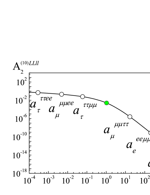
Figure 3: The tenth order coefficients $\displaystyle A_{2}^{(10)LL\ell\ell}(r)$, Eqs. (III.1)–(30), as a function of the ratio $\displaystyle r=m_{\ell}/m_{L}$, for the external lepton $\displaystyle L$ with the insertions of the polarizationoperators with four loops. The notation $\displaystyle A_{2}^{(10)LL\ell\ell}(r)$ indicates that the four loops correspond to two leptons $\displaystyle L$ and two leptons $\displaystyle\ell$ ($\displaystyle L,\ell=e,\mu$ and $\displaystyle\tau$). The open circles, as well as the associated with them labels, point to physical values of the ratio $\displaystyle r$ and to the corresponding physical coefficients $\displaystyle A^{(10)LL\ell\ell}(r)$. The universal value $\displaystyle A_{2}^{(10)}(r=1)$ is displayed by the full circle.

The results of numerical calculations are presented in Fig. 3 for the coefficients $\displaystyle{{\ A}}_{2}^{(10),LL\ell\ell}(r)$, Eq. (14), which are displayed as a function of $\displaystyle r$ (solid line), where $\displaystyle r$ ranges in the interval $\displaystyle 0<\,r\,<\,\infty$. The open circles, accompanied by the corresponding labels $\displaystyle a_{L}^{LL\ell\ell}$, denote all the possible combinations of the real existing leptons $\displaystyle L$ and $\displaystyle\ell$ ($\displaystyle L,\ell=e,\mu$ and $\displaystyle\tau$). The full circle corresponds to $\displaystyle r=1$, i.e., to the universal coefficient $\displaystyle A_{2}^{(10),LL\ell\ell}(r=1)=6A_{1}^{(10)}\simeq 0.00282543429618$, cf. Eq. (16).

It can be seen from Fig. 3 that the corrections $\displaystyle A_{2}^{(10),LL\ell\ell}(r)$ for the anomaly of the lepton $\displaystyle L$ basically come from the region $\displaystyle r<1$, i.e. from diagrams with loops formed by leptons $\displaystyle\ell$ lighter than the external one. Moreover, they are larger than the universal coefficients at $\displaystyle r=1$. Contributions from loops with leptons $\displaystyle\ell$ heavier than the lepton $\displaystyle L$ rapidly decreasing with increase $\displaystyle r$ and can be by 10–11 orders of magnitude below the universal value. Note that, since the large scale of the ordinate axis, more than 18 orders of magnitude), Fig. 3 illustrates only qualitatively the main features of the tenth order corrections. For precise calculations of $\displaystyle A_{2}^{(10),LL\ell\ell}(r)$, one should use directly the analytical forms presented in Eqs. (III.1)–(30).

V Asymptotic expansions

As mentioned, the tenth order corrections in the literature have been considered analytically only as limiting expansions $\displaystyle r\ll 1$ cf. Refs. Aguilar:2008qj ; Laporta94 and only for muons, i.e., only diagrams with electron internal loops have been included into the consideration. Since Eqs. (III.1)–(29) provide exact analytical expressions for the QED corrections from the diagrams in Fig. 2, we can calculate the corresponding limits not only at $\displaystyle r\ll 1$ but also at $\displaystyle r\gg 1$ for any type of leptons $\displaystyle L$ and $\displaystyle\ell$. The results of expansions can be then compared with the expansions presented in Refs. Aguilar:2008qj ; Laporta94 . To make the comparison with Refs. Aguilar:2008qj ; Laporta94 easier, below we present the asymptotic expansions in terms of the variable $\displaystyle t\equiv r^{2}$. The corresponding expansions of Eqs. (III.1)–(30) read as:

Eq. (III.1), $\displaystyle t=r^{2}\ll 1$.

$$\displaystyle A_{2,asymp.}^{(10)}(t)\underset{t\ll 1}{=}\;\left(-\frac{943}{486}-\frac{8}{405}\pi^{2}+\frac{16}{9}\zeta(3)\right)\ln^{2}t-\left(\frac{57899}{7290}-\frac{10766}{6075}\pi^{2}+\frac{8}{81}\pi^{4}-\frac{8}{135}\zeta(3)\right)$$

$$\displaystyle~{}~{}~{}\times\ln t-\frac{1090561}{109350}-\frac{148921}{91125}\pi^{2}-\frac{106}{6075}\pi^{4}+\frac{10732}{2025}\zeta(3)+\frac{32}{27}\pi^{2}\zeta(3)+\frac{64}{9}\zeta(5)$$

$$\displaystyle+\left[-\left(\frac{1832}{243}-\frac{104}{315}\pi^{2}-\frac{32}{9}\zeta(3)\right)\ln t-\frac{619798}{25515}+\frac{564008}{297675}\pi^{2}-\frac{8}{81}\pi^{4}+\frac{1328}{105}\zeta(3)\right]t$$

$$\displaystyle+\left[\left(\frac{29696}{45927}+\frac{852346}{535815}\pi^{2}-\frac{8}{81}\pi^{4}-\frac{3224}{567}\zeta(3)\right)\ln t-\left(\frac{470}{729}+\frac{260}{1701}\pi^{2}-\frac{16}{9}\zeta(3)\right)\ln^{2}t\right.$$

$$\displaystyle+\left.\frac{51445307}{28934010}-\frac{546693856}{168781725}\pi^{2}+\frac{26}{729}\pi^{4}+\frac{752123}{178605}\zeta(3)+\frac{32}{27}\pi^{2}\zeta(3)+\frac{64}{9}\zeta(5)\right]t^{2}$$

$$\displaystyle+\left[\frac{244420473203}{72937816875}-\frac{186003297484\pi{{}^{2}}}{374414126625}+\frac{64\pi^{4}}{2475}-\left(\frac{94530074}{105249375}-\frac{7124144\pi^{2}}{108056025}-\frac{256}{385}\zeta(3)\right)\right.$$

$$\displaystyle\left.\times\ln(t)-\left(\frac{11114}{30375}-\frac{64\pi^{2}}{1155}\right)\ln^{2}(t)+\frac{32}{2025}\ln^{3}(t)+\frac{14248288}{36018675}\zeta(3)\right]t^{3}+{\cal{O}}\left(t^{4}\ln^{4}t\right).$$ (31)

Our expansion (31) can be directly compared term by term with their analogues presented in Refs. Aguilar:2008qj ; Laporta94 . A meticulous inspection of expansions (V) with their analogues in Ref. Aguilar:2008qj (Eq. (A13)) and Ref. Laporta94 (Eq. (3)) shows that the term $\displaystyle\frac{64}{9}\zeta(5)$ is absent in Ref. Aguilar:2008qj . Besides, there is another misprint in Ref. Aguilar:2008qj , namely the term

$$-\left[\left(\frac{470}{729}+\frac{260}{1701}\pi^{2}-\frac{16}{9}\zeta(3)\right)\ln^{2}t\right]t^{2}$$

has been omitted.

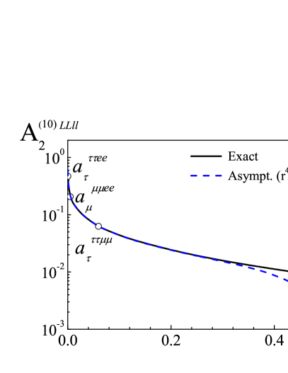
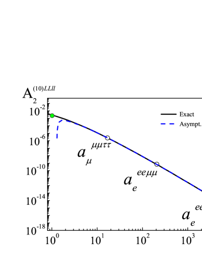
Figure 4: The asymptotic expansion of the coefficients $\displaystyle A_{2}^{(10)\ LL\ell\ell}$, dashed lines, vs. the exact calculations by Eqs. (III.1)–(30), solid lines. Left panel: $\displaystyle r<1$; Right panel $\displaystyle r>1$. The meaning of the open circles and labels $\displaystyle a_{L}^{LL\ell\ell}$ is the same as in Fig. 3.

Eq. (29), $\displaystyle t=r^{2}\gg 1$.

$$\displaystyle A_{2,asymp.}^{(10)}(t)\underset{t\gg 1}{=}\;\left(\frac{6938293}{29160000}+\frac{20327}{2430000}\ln t-\frac{61}{81000}\ln^{2}t+\frac{2}{2025}\ln^{3}t-\frac{136}{675}\zeta(3)\right)\frac{1}{t^{2}}$$ (32)

$$\displaystyle+\left(\frac{1364352509}{87516450000}+\frac{675182}{52093125}\ln t-\frac{6073}{1488375}\ln^{2}t+\frac{2}{1375}\ln^{3}t-\frac{8}{525}\zeta(3)\right)\frac{1}{t^{3}}+{\cal{O}}\left(\frac{1}{t^{4}}\right).$$

The comparisons of the limiting expansions $\displaystyle r\to 0$, Eq. (V), and $\displaystyle r\to\infty$, Eq. (32), with exact numerical calculations by Eqs. (III.1)–(30) are presented in Fig. 4. One can conclude that the approximate expansions practically coincide with the exact formulae in quite large intervals of $\displaystyle r$, namely $\displaystyle(0<r<0.2)$ for the expansion (31) and $\displaystyle(4<r<\infty)$ for the expansion (32), herewith both intervals include all the corresponding physical values of $\displaystyle a_{L}^{LL\ell\ell}$. It means that in these intervals qualitative estimates of the corrections to any type of leptons can be safely performed by asymptotic expansions instead of the exact but cumbersome expressions Eqs. (III.1)–(30).

VI Summary

In summary, we have derived, for the first time, analytical expressions of the QED corrections $\displaystyle A_{2}^{(10)}(r)$ of the tenth order to the anomalous magnetic moment of leptons $\displaystyle L$ ($\displaystyle L=e,\mu$ or $\displaystyle\tau$ ) generated by diagrams with insertions of four loops in the photon vacuum polarization operator. We considered the diagram with loops formed by two leptons $\displaystyle L$ of the same type as the external one and two leptons $\displaystyle\ell$ different from $\displaystyle L$. The radiative corrections have been obtained in close analytical forms in terms of the mass ratio $\displaystyle r=\frac{m_{\ell}}{m_{L}}$. The generic variable $\displaystyle r$ is defined in the whole region $\displaystyle(0<r<\infty)$. Our consideration is based on a combined use of the dispersion relations for the vacuum polarization operators and the Mellin–Barnes integral transform for the Feynman parametric integrals. This technique is widely used in the literature in multi-loop calculations in relativistic quantum field theories, c.f. Refs. Friot:2005cu ; Rafael-HVP ; Kotikov:2018wxe . The final integrations have been performed by the Cauchy residue theorem in the left ($\displaystyle r<1$) and right ($\displaystyle r>1$) semiplanes of the complex Mellin variable $\displaystyle s$. We investigated numerically the behaviour of the corrections $\displaystyle A_{2}^{(10)}(r)$ in the whole interval $\displaystyle 0<r<\infty$ for all possible combinations of the two leptons $\displaystyle L$ and two $\displaystyle\ell$. We found that the contributions to $\displaystyle A_{2}^{(10)}(r)$ basically come from the region $\displaystyle r<1$, i.e. from diagrams with loops formed by leptons $\displaystyle\ell$ lighter than the external one. Moreover, these corrections are larger than the universal coefficients at $\displaystyle r=1$. Contributions from loops with leptons $\displaystyle\ell$ heavier than the lepton $\displaystyle L$ rapidly decrease with increasing $\displaystyle r$ and can be by 10–11 orders of magnitude below the universal value.

We have compared our analytical expressions the corresponding asymptotic expansions with the well-known results available in the literature and found that our results are fully compatible with the earlies known calculations. We also argued that the asymptotic expansions in the regions $\displaystyle r<0.2$ and $\displaystyle r>4$ are rather close to the exact values and can serve as reliable estimates of $\displaystyle A_{2}^{(10)}(r)$ in these regions.

References

- (1) P. A. M. Dirac, The quantum theory of the electron, Proc. Roy. Soc. Lond. A 117, 610 (1928).
- (2) F. Jegerlehner, The anomalous magnetic moment of the muon, Springer Tracts Mod. Phys. 274, 693 (2017).
- (3) T. Aoyama et al., The anomalous magnetic moment of the muon in the Standard Model, Phys. Rep. 887, 1 (2020).
- (4) R. H. Parker, C. Yu, W. Zhong, B. Estey and H. Meller, Measurement of the fine-structure constant as a test of the Standard Model, Science 360, 191 (2018).
- (5) L. Morel, Z. Yao, P. Clad et al., Determination of the fine-structure constant with an accuracy of 81 parts per trillion, Nature 588, 61 (2020).
- (6) B. Abi et al. (Muon Collaboration), Measurement of the Positive Muon Anomalous Magnetic Moment to 0.46 ppm, Phys. Rev. Lett. 126, 141801 (2021).
- (7) D. P. Aguillard et al. (Muon Collaboration), Measurement of the Positive Muon Anomalous Magnetic Moment to 0.20 ppm, FERMILAB-PUB-23-385-AD-CSAID-PPD, e-Print: 2308.06230 [hep-ex].
- (8) J. S. Schwinger, On Quantum electrodynamics and the magnetic moment of the electron, Phys. Rev. 73, 416 (1948); Quantum electrodynamics. III: The electromagnetic properties of the electron: radiative corrections to scattering, Phys. Rev. 76, 790 (1949).
- (9) A. Petermann, Fourth order magnetic moment of the electron, Helvetica Physica Acta. 30, 407 (1957).
- (10) C. M. Sommerfield, Magnetic dipole moment of the electron, Phys. Rev. 107, 328 (1957).
- (11) H. R. P. Ferguson and D. H. Bailey, A polynomial time, numerically stable integer relation algorithm, RNR Technical Report RNR-91-032.
- (12) S. Laporta, The analytical contribution of some eighth order graphs containing vacuum polarization insertions to the muon in QED, Phys. Rev. B 312, 495 (1993).
- (13) S. Laporta, High-precision calculation of the 4-loop contribution to the electron g-2 in QED, Phys. Rev. B 772, 232 (2017).
- (14) V. B. Berestetskii, O. N. Krohnin and A. K. Khlebnikov, Concerning the radiative corrections to the -meson magnetic moment, Zh. Eksp. Teor. Fiz., 30, 788 (1956) [Sov. Phys. JETP, 3, 761 (1956)].
- (15) S. J. Brodsky and E. de Rafael, Suggested boson-lepton pair coupling and the anamalous magnetic moment of the muon, Phys. Rev. 168, 1620 (1968).
- (16) O. P. Solovtsova, V. I. Lashkevich and L. P. Kaptari, Lepton anomaly from QED diagrams with vacuum polarization insertions within the Mellin–Barnes representation, Eur. Phys. J. Plus 138, 212 (2023).
- (17) J. P. Aguilar, D. Greynat and E. de Rafael, Muon anomaly from lepton vacuum polarization and the Mellin-Barnes representation, Phys. Rev. D 77, 093010 (2008).
- (18) V.I. Laskevich, O.P. Solovtsova and L.P. Kaptari, Proc. of the National Academy of Sciences of Belarus. Physics and Mathematics series 59, 2023 (to be published).
- (19) B. E. Lautrup and E. de Rafael, Calculation of the sixth-order contribution from the fourth-order vacuum polarization to the difference of the anomalous magnetic moments of muon and electron, Phys. Rev. 174, 1835 (1968).
- (20) I. Dubovyk, J. Gluza and G. Somogyi, Mellin-Barnes Integrals: A Primer on Particle Physics Applications, Lect. Notes Phys. 1008, 208 (2022).
- (21) V. A. Smirnov, Analytic tools for Feynman integrals, Springer Tracts Mod. Phys. 250, 1 (2012).
- (22) E. E. Boos and A. I. Davydychev, A method of evaluation massive Feynman diagrams, Theor. Math. Phys. 89, 1052 (1991).
- (23) M. L. Laursen and M. A. Samuel, The -bubble diagram contribution to of the electron mathematical structure of the analytical expression, Phys. Lett. B 91, 249 (1980); The -bubble diagram contribution to , J. Math. Phys. 22, 1114 (1981).
- (24) S. Laporta, New results on calculation, J. Phys. Conf. Ser. 1085, 022004 (2018); Four-loop QED contributions to the electron , J. Phys. Conf. Ser. 1138, 012001 (2018).
- (25) S. Laporta and E. Remiddi, The analytical value of the electron at order in QED, Phys. Lett. B 379, 283 (1996).
- (26) B. Latrup, On high order estimates in QED, Phys. Lett. 69B, 109 (1977).
- (27) V. I. Lashkevich, O. P. Solovtsova and O. V. Teryaev, On high order contributions to the anomalous magnetic moments of leptons due to the vacuum polarization by lepton loops. Proc. of the National Academy of Sciences of Belarus. Physics and Mathematics series, 58, 412 (2022) (in Russian).
- (28) V. I. Lashkevich, O. P. Solovtsova and L. P. Kaptari, work in progress.
- (29) S. Laporta, Analytical and numerical contributions of some tenth-order graphs containing vacuum polarization insertions to the muon in QED, Phys. Lett. B 328, 522 (1994).
- (30) S. Friot, D. Greynat and E. de Rafael, Asymptotics of Feynman diagrams and the Mellin-Barnes representation, Phys. Lett. B 628, 73 (2005).
- (31) J. Charles, E. de Rafael and D. Greynat, Mellin-Barnes approach to hadronic vacuum polarization and , Phys. Rev. D 97, 076014 (2018).
- (32) A. V. Kotikov and S. Teber, Multi-loop techniques for massless Feynman diagram calculations, Phys. Part. Nucl. 50, 1 (2019).