Learning to Generate Parameters of ConvNets for Unseen Image Data

Abstract

Typical Convolutional Neural Networks (ConvNets) depend heavily on large amounts of image data and resort to an iterative optimization algorithm (e.g., SGD or Adam) to learn network parameters, which makes training very time- and resource-intensive. In this paper, we propose a new training paradigm and formulate the parameter learning of ConvNets into a prediction task: given a ConvNet architecture, we observe there exists correlations between image datasets and their corresponding optimal network parameters, and explore if we can learn a hyper-mapping between them to capture the relations, such that we can directly predict the parameters of the network for an image dataset never seen during the training phase. To do this, we put forward a new hypernetwork based model, called PudNet, which intends to learn a mapping between datasets and their corresponding network parameters, and then predicts parameters for unseen data with only a single forward propagation. Moreover, our model benefits from a series of adaptive hyper recurrent units sharing weights to capture the dependencies of parameters among different network layers. Extensive experiments demonstrate that our proposed method achieves good efficacy for unseen image datasets on two kinds of settings: Intra-dataset prediction and Inter-dataset prediction. Our PudNet can also well scale up to large-scale datasets, e.g., ImageNet-1K. It takes 8967 GPU seconds to train ResNet-18 on the ImageNet-1K using GC from scratch and obtain a top-5 accuracy of 44.65 %. However, our PudNet costs only 3.89 GPU seconds to predict the network parameters of ResNet-18 achieving comparable performance (44.92 %), more than 2,300 times faster than the traditional training paradigm.

I Introduction

Convolutional Neural Networks (ConvNets) have yielded superior performance in a variety of fields in the past decade, such as computer vision [1], reinforcement learning [2, 3], etc. One of the keys to success for ConvNets stems from huge amounts of image training data. In order to optimize ConvNets, the traditional training paradigm takes advantage of an iterative optimization algorithm (e.g., SGD) to train the model in a mini-batch manner, leading to huge time and resource consumption. For example, when training ResNet-101 [4] on ImageNet [5], it often takes several days or weeks for the model to be well optimized with GPU involved. Thus, how to accelerate the training process of ConvNets is an emergent topic in deep learning.

Nowadays, many methods for accelerating training of deep neural networks have been proposed [6, 7, 8]. The representative works include optimization based techniques by improving the stochastic gradient descent [6, 9, 10], normalization based techniques [7, 11, 12], parallel training techniques [8, 13], et. Although these methods have showed promising potential to speed up the training of the network, they still follow the traditional iterative-based training paradigm.

In this paper, we investigate a new training paradigm for ConvNets. In contrast to previous works accelerating the training of the network, we formulate the parameter training problem into a prediction task: given a ConvNet architecture, we attempt to learn a hyper-mapping between image datasets and their corresponding optimal network parameters, and then leverage the hyper-mapping to directly predict the network parameters for a new image dataset unseen during training. A basic assumption behind the above prediction task is that there exists correlations between image datasets and their corresponding parameters of a given ConvNet.

Figure 1: Correlation coefficients between training datasets and the network parameters on the Fashion-MNIST [14], CIFAR-100 [15], Mini-ImageNet [16] datasets, respectively.‘learned’ depicts correlations between training datasets and the corresponding optimal network parameters. ‘random’ denotes correlations between training datasets and the network parameters selected randomly from 1000 groups.

In order to demonstrate the rationality of this assumption, we perform the following experiment: for an image dataset, we first randomly sample 3000 images to train a 3-layer convolutional neural network until convergence. Then we conduct the average pooling operation to the original inputs as a vector representation of the training data. We repeat the above experiment 1000 times, and thus obtain 1000 groups of representations and the corresponding network parameters. Finally, we utilize Canonical Correlation Analysis (CCA) [17] to evaluate the correlations between training data and the network parameters by the above 1000 groups of data. Fig. 1 shows the results, which illustrates there are indeed correlations between training datasets and their network parameters for a given network architecture.

In light of this, we propose a new hypernetwork based model, called PudNet, to learn a hyper-mapping between image datasets and ConvNet parameters. Specifically, PudNet first summarizes the characters of image datasets by compressing them into different vectors as their sketch. Then, PudNet extends the traditional hypernetwork [18] to predict network parameters of different layers based on these vectors. Considering that model parameters among different layers should be not independent, we design an adaptive hyper recurrent unit (AHRU) sharing weights to capture the relations among them. This design allows the predicted parameters of each layer to adapt to both the dataset-specific information and the predicted parameter information from previous layers, resulting in an enhanced performance of PudNet. Finally, it is worth noting that for training PudNet, it is prohibitive if preparing thousands of datasets and training the network of a given architecture on these datasets to obtain the corresponding optimal parameters respectively. Instead, we adopt a meta-learning based approach  [19] to train the hypernetwork.

In the experiment, our PudNet showcases the remarkable efficacy for unseen yet related image datasets. For example, it takes around 54, 119, 140 GPU seconds to train ResNet-18 using Adam from scratch and obtain top-1 accuracies of 99.91%, 74.56%, 71.84% on the Fashion-MNIST [14], CIFAR-100 [15], Mini-ImageNet [16], respectively. While our method costs only around 0.5 GPU seconds to predict the parameters of ResNet-18 and still achieves 96.24%, 73.33%, 71.57% top-1 accuracies on the three datasets respectively, at least 100 times faster than the traditional training paradigm. More surprisingly, PudNet exhibits impressive performance even on cross-domain unseen image datasets, demonstrating good generalization ability of PudNet.

Our contributions are summarized as follows:

• We find there are correlations between image datasets and their corresponding parameters of a given ConvNet, and propose a general training paradigm for ConvNets by formulating network training into a prediction task.

• We extend hypernetwork to learn the correlations between image datasets and the corresponding ConvNet parameters, such that we can directly generate parameters for unseen image data with only a single forward propagation. Furthermore, a theoretical analysis of the hyper-mapping is provided to offer interpretability.

• We design an adaptive hyper recurrent unit that empowers the predicted parameters of each layer to encompass both the dataset-specific information and the inter-layer parameter dependencies.

• We perform extensive experiments on image datasets in terms of both Intra-dataset and Inter-dataset prediction tasks, demonstrating the efficacy of our method. We expect that such results can motivate more researchers to explore along with this research direction.

II Related work

II-A Hypernetwork

Hypernetwork in [18] aims to decrease the number of training parameters, by training a smaller network to generate the parameters of a larger network on a fixed dataset. Hypernetwork has been gradually applied to various tasks [20, 21, 22, 23, 24, 25, 26, 27]. [22] proposes a task-conditioned hypernetwork to overcome catastrophic forgetting in continual learning. Bayesian hypernetwork [20] is proposed to approximate Bayesian inference in neural networks. [28] and [29] utilize many layer-wise hypernetworks shared by different tasks to generate weights for the adapters [30] of different layers. GHN-2 proposed in [31] attempts to build a mapping between the network architectures and network parameters, where the dataset is always fixed. HyperTransformer [32] adopts a transformer-based hypernetwork to blend the information of a small support set to generate parameters for a small CNN in the few-shot setting. However, due to the high time complexity of the attention operation, this approach faces the scalability issue as networks become deeper and the support set becomes larger. Different from these works, we aim to directly predict the parameters of a given ConvNet for unseen image datasets.

II-B Acceleration of Network Training

Many works have been proposed to speed up the training of deep neural networks, including optimization based methods [33, 6, 9], normalization based methods [7, 12, 11], parallel training methods [8, 13, 34], etc. Optimization based methods mainly aim to improve the stochastic gradient descent. For instance, Adaptive Moment Estimation (Adam) [6] achieves this by combining the strengths of AdaGrad [33] and RMSProp [35]. By comprehensively considering both the first-order moment estimation and the second-order moment estimation of the gradients, Adam [6] enables the utilization of more efficient and adaptive learning rates for each parameter. [9] proposes a gradient centralization method that centralizes gradient vectors to improve the Lipschitzness of the loss function. Normalization based methods intend to design good normalization methods to speed up training. The representative work is batch normalization [7] that can make optimization the landscape smooth and lead to fast convergence [36]. Parallel training methods [34, 37] usually stack multiple hardwares to conduct parallel training, which reduces training time by dispersing calculation amounts to distributed devices. However, these methods still follow the traditional iterative based training paradigm. Different from them, we attempt to explore a new training paradigm, and transform the network training problem into a parameter prediction task.

II-C Meta-Learning

Meta-learning (a.k.a. learning to learn) aims to learn a model from a variety of tasks, such that it can quickly adapt to a new learning task using only a small number of training samples [38]. So far, many meta-learning methods have been proposed [39, 40, 38, 41, 42]. The representative algorithms include optimization-based methods and metric-based methods [38]. Optimization-based meta-learning methods usually train the model for easily finetuning by a small number of gradient steps [19, 43]. Metric-based meta-learning methods attempt to learn to match the training sets with the class centroids and predict the label of training sets with the matched classes [40, 44, 45]. Because of its powerful ability, meta-learning has been widely used for various tasks, including few-shot learning [16, 40, 46, 45], zero-shot learning [47], etc. Different from the above methods, we propose a new training paradigm of neural networks, where we attempt to directly predict network parameters for an unseen dataset with only a single forward propagation without training on the dataset.

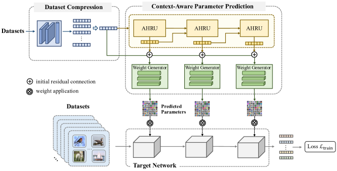
Figure 2: Overview of our PudNet. PudNet compresses each image dataset into a sketch with a fixed size, and then utilizes the designed hypernetwork to generate parameters of a target ConvNet by the sketch. Specifically, PudNet exploits the adaptive hyper recurrent units (AHRU) to process the dataset sketch, capturing the dependencies of parameters among different network layers for predicting the parameter representations. Subsequently, the weight generators are employed to produce the dataset-specific parameters of the target ConvNet.

III Proposed Method

III-A Preliminaries and Problem Formulation

We denote $H_{\theta}$ as our hypernetwork parameterized by $\theta$. Let $\mathcal{D}^{train}=\{D_{i}\}_{i=1}^{\mathcal{N}}$ be the set of image training datasets, where $D_{i}$ is the $i^{th}$ image dataset and $\mathcal{N}$ is the number of image training datasets. Each sample $x_{j}\in D_{i}$ has a label $y_{j}\in\mathcal{C}^{tr}_{i}$, where $\mathcal{C}^{tr}_{i}$ is the class set of $D_{i}$. We use $\mathcal{C}^{tr}=\bigcup_{i=1}^{\mathcal{N}}\mathcal{C}^{tr}_{i}$ to denote the whole label set of image training datasets. Similarly, we define $\mathcal{D}^{test}$ as the set of unseen image datasets used for testing and $\mathcal{C}^{te}$ as the set containing all labels in $\mathcal{D}^{test}$.

In contrast to traditional iterative-based training paradigm, we attempt to explore a new training paradigm, and formulate the training of ConvNets into a parameter prediction task. To this end, we propose the following objective function:

$$\mathop{\arg\min}\limits_{\theta}\quad\sum_{i=1}^{\mathcal{N}}\mathcal{L}(\mathcal{F}(D_{i},\Omega;H_{\theta}),\mathcal{M}_{i}^{\Omega}),$$ (1)

where $\mathcal{F}(D_{i},\Omega;H_{\theta})$ denotes a forward propagation of our hypernetwork $H_{\theta}$. The input of the forward propagation is the dataset $D_{i}$ and its output is the predicted parameters of ConvNet $\Omega$ by $H_{\theta}$. Note that the architecture of $\Omega$ is always fixed during training and testing, e.g., ResNet-18. This makes sense because we often apply a representative deep model to data of different domains. Thus, it is obviously meaningful if we can predict the network parameters for unseen image data using an identical network architecture. $\mathcal{M}^{\Omega}=\{\mathcal{M}_{i}^{\Omega}\}_{i=1}^{\mathcal{N}}$ denotes the ground-truth parameter set of ConvNet $\Omega$ corresponding to image datasets $\mathcal{D}^{train}$, where $\mathcal{M}_{i}^{\Omega}$ is the ground-truth parameters for the dataset $D_{i}$. $\mathcal{L}$ is a loss function, measuring the difference between the ground-truth parameters $\mathcal{M}_{i}^{\Omega}$ and the predicted parameters.

The core idea in (1) is to learn a hyper-mapping $H_{\theta}$ between image datasets $\mathcal{D}^{train}$ and the ConvNet parameter set $\mathcal{M}^{\Omega}$, on the basis of our finding that there are correlations between image datasets and the ConvNet parameters, as shown in Fig. 1. However, it is prohibitive if preparing thousands of image datasets $D_{i}$ and training $\Omega$ on $D_{i}$ to obtain the corresponding ground-truth parameters $\mathcal{M}_{i}^{\Omega}$ respectively. To alleviate this problem, we adopt a meta-learning based [16] approach to train the hypernetwork $H_{\theta}$, and propose another objective function as:

$$\mathop{\arg\min}\limits_{\theta}\quad\sum_{i=1}^{\mathcal{N}}\sum_{x_{j}\in D_{i}}\mathcal{L}(x_{j},y_{j};\mathcal{F}(D_{i},\Omega;H_{\theta})),$$ (2)

Instead of optimizing $H_{\theta}$ by directly matching the predicted parameters $\mathcal{F}(D_{i},\Omega;H_{\theta})$ with the ground-truth parameters $\mathcal{M}_{i}^{\Omega}$, we can adopt a typical loss, e.g., cross-entropy, to optimize $H_{\theta}$, where each dataset $D_{i}$ can be regarded as a task in meta-learning [16]. By learning on multiple tasks, the parameter predictor $H_{\theta}$ is gradually able to learn to predict performant parameters for training datasets $\mathcal{D}^{train}$. During testing, we can utilize $\mathcal{F}(D,\Omega;H_{\theta})$ to directly predict the parameters for a dataset $D$ never seen in $\mathcal{D}^{train}$ with only a single forward propagation without training on $D$.

III-B Overview of Our Framework

Our goal is to learn a hypernetwork $H_{\theta}$, so as to directly predict the ConvNet parameters for an unseen image dataset by $H_{\theta}$. However, there remains two issues that are not solved: First, the sizes of different $D_{i}$ may be different and the dataset sizes may be large, which makes $H_{\theta}$ hard to be trained; Second, there may be correlations among parameters of different layers in a network. However, how to capture such context relations among parameters has not been fully explored so far.

To this end, we propose a novel framework, PudNet, as shown in Fig. 2, PudNet first introduces a dataset compression module to compress each dataset $D_{i}$ into a small size sketch $\mathbf{s}_{i}$ to summarize the major characteristics of $D_{i}$. Then, our context-aware parameter prediction module takes the sketch $\mathbf{s}_{i}$ as input, and outputs the predicted parameters of the target network, e.g., ResNet-18. In addition, multiple adaptive hyper recurrent units sharing weights are constructed to capture the dependencies of parameters among different layers of the network. Finally, PudNet is optimized in a meta-learning based manner.

III-C Dataset Compression

To solve the issue of different sizes of training datasets, we first compress each image dataset into a sketch with a fixed size. In recent years, many data compression methods have been proposed, such as matrix sketching [48, 49], random projection [50], etc. In principle, these methods can be applied to our data compression module. For simplification, we leverage a neural network to extract a feature vector as the representation of each sample, and then conduct the average pooling operation to generate a final vector as the sketch of the dataset. The sketch $\mathbf{s}_{i}$ for the dataset $D_{i}$ can be calculated as:

$$\mathbf{s}_{i}=\frac{1}{|D_{i}|}\sum_{x_{j}\in D_{i}}T_{\phi}(x_{j}),\quad D_{i}\in\{D_{i}\}_{i=1}^{\mathcal{N}},$$ (3)

where $T_{\phi}(\cdot)$ denotes a feature extractor parameterized by $\phi$, and $|D_{i}|$ is the size of the dataset $D_{i}$. The parameter $\phi$ is jointly trained with PudNet in an end-to-end fashion. In our PudNet, the feature extractor contains three basic blocks, where each basic block consists of a $5\times 5$ convolutional layer, a leakyReLU function and a batch normalization layer. For future work, more efforts could be made to explore more effective solutions to summarize the information of a dataset, e.g. using statistic network [51] to compress datasets.

III-D Context-Aware Parameter Prediction

After obtaining the sketches for all training datasets, we will feed them into the context-aware parameter prediction module, as shown in Fig. 2. In the followings, we will introduce this module in detail.

III-D1 Capturing Contextual Parameter Relations via Adaptive Hyper Recurrent Units

First, since we aim to establish a hypernetwork that can capture the hyper-mapping between datasets and their corresponding network parameters, the hypernetwork should be adaptive to different datasets, so as to predict dataset-specific parameters. Second, as the input of a neural network would sequentially pass forward its layers, the parameters of different layers should be not independent. Neglecting the contextual relations among parameters of different layers may result in sub-optimal solutions.

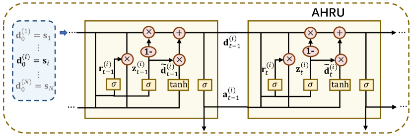
Figure 3: An illustration of capturing context relations via AHRU.

In light of this, we construct Adaptive Hyper Recurrent Units (AHRU), specifically designed for parameter prediction of ConvNets. AHRU enhances the capabilities of the gated recurrent unit by adapting to different datasets, while also acting as the hyper recurrent unit to capture context-aware parameter relations during the parameter generation process. As shown in Fig. 3, we set the dataset sketch embeddings $\mathbf{s}_{i}$ as the input of the hyper recurrent unit:

$$\mathbf{d}_{0}^{(i)}=\mathbf{s}_{i},\quad\mathbf{s}_{i}\in\{\mathbf{s}_{i}\}_{i=1}^{\mathcal{N}},$$ (4)

where $\mathbf{d}_{0}^{(i)}$ represents the initial hidden state of AHRU. In this way, we can integrate dataset-specific information into parameter prediction.

Then, we predict parameter representation $\mathbf{a}_{t}^{(i)}$ of $t$-th layer in $\Omega$ for the $i$-th dataset as follows:

$$\mathbf{r}_{t}^{(i)}=\sigma(\mathbf{W}_{r}\cdot[\mathbf{d}_{t-1}^{(i)},\mathbf{a}_{t-1}^{(i)}]),$$

$$\mathbf{z}_{t}^{(i)}=\sigma(\mathbf{W}_{z}\cdot[\mathbf{d}_{t-1}^{(i)},\mathbf{a}_{t-1}^{(i)}]),$$

$$\tilde{\mathbf{d}}_{t}^{(i)}=tanh(\mathbf{W}_{h}\cdot[\mathbf{r}_{t}^{(i)}\ast\mathbf{d}_{t-1}^{(i)},\mathbf{a}_{t-1}^{(i)}]),$$

$$\mathbf{d}_{t}^{(i)}=(1-\mathbf{z}_{t}^{(i)})\ast\mathbf{d}_{t-1}^{(i)}+\mathbf{z}_{t}^{(i)}\ast\tilde{\mathbf{d}}_{t}^{(i)},$$

$$\mathbf{a}_{t}^{(i)}=\sigma(\mathbf{W}_{o}\cdot\mathbf{d}_{t}^{(i)}),$$

where $\mathbf{d}_{t-1}^{(i)}$ serves as the hidden state in AHRU for conveying both dataset-related context information specific to the $i$-th dataset and parameter information from previous layers. $\mathbf{W}_{r},\mathbf{W}_{z},\mathbf{W}_{h},\mathbf{W}_{o}$ are learnable parameters shared by different datasets. In AHRU, the reset gate $\mathbf{r}_{t}^{(i)}$ decides how much data information in hidden state $\mathbf{d}_{t-1}^{(i)}$ needs to be reset. $\tilde{\mathbf{d}}_{t}^{(i)}$ is a new memory, which absorbs the information of $\mathbf{d}_{t-1}^{(i)}$ and $\mathbf{a}_{t-1}^{(i)}$. $\mathbf{z}_{t}$ is an update gate, which regulates how much information in $\tilde{\mathbf{d}}_{t}^{(i)}$ to update and how much information in $\mathbf{d}_{t-1}^{(i)}$ to forget. During this process, the hidden state $\mathbf{d}_{t-1}^{(i)}$ along with the parameter representation $\mathbf{a}_{t-1}^{(i)}$ in the previous layer are utilized to produce $\mathbf{a}_{t}^{(i)}$. By doing so, $\mathbf{a}_{t}^{(i)}$ can effectively encompass the dependency information between different layers while also adapting to the $i$-th dataset. The derived parameter representation $\mathbf{a}_{t}^{(i)}$ will be taken as input to the weight generator to predict parameters of the $t$-th layer of the target network $\Omega$.

It’s worth noting that AHRU is designed based on the GRU-based architecture [52] but differs from the traditional GRU. Our AHRU is capabale of adapting to various datasets according to the dataset sketches, as well as capturing the dependencies among parameters of different layers. Specifically, conventional GRU utilizes the randomly initialized hidden state to carry the long-term memory. In each recurrent step, it needs to receive external input (e.g., word) to update the hidden state and capture the contextual information. Instead of that, we set each dataset sketch embedding as input and follow a self-loop structure to incorporate the predicted structure parameter representation from the previous layer. This approach allows us to leverage the dataset-specific information and meanwhile enables the information of shallower layer parameters to help the prediction of parameters in the deeper layer. By utilizing AHRU, our PudNet possesses the ability to adapt to various datasets, and the dependencies among parameters of different layers can be well captured.

III-D2 Initial Residual Connection

To ensure that the final context-aware output contains at least a fraction of the initial dataset information, we additionally implement an initial residual connection between dataset sketch embedding $\mathbf{s}_{i}$ and $\mathbf{a}_{t}$ as:

$$\hat{\mathbf{a}}_{t}^{(i)}=\mathbf{a}_{t}^{(i)}\times(1-\eta)+\mathbf{s}_{i}\times\eta,\quad\hat{\mathbf{a}}_{t}^{(i)}\in\mathbb{R}^{m},$$ (5)

where $\eta$ is the hyperparameter. After obtaining $\hat{\mathbf{a}}_{t}^{(i)}$, we put $\hat{\mathbf{a}}_{t}^{(i)}$ into the weight generator to generate parameters of the $t$-th layer of the target network $\Omega$.

III-D3 Weight Generator

Since the target network $\Omega$ usually has different sizes and dimensions in different layers, we construct the weight generator $g_{\psi_{t}}$ for each layer $t$ to transform $\hat{\mathbf{a}}_{t}^{(i)}$ of a fixed dimension to network parameter tensor $\mathbf{w}_{t}^{(i)}$ with variable dimensions. Here $g_{\psi_{t}}$ denotes the weight generator of the $t$-th layer, $\psi_{t}$ is the learnable parameters of $g_{\psi_{t}}$, $\mathbf{w}_{t}^{(i)}$ is the predicted parameter of the $t$-th layer in $\Omega$ for the $i$-th dataset. We can derive the predicted parameter of the $t$-th layer as:

$$\mathbf{w}_{t}^{(i)}=g_{\psi_{t}}(\hat{\mathbf{a}}_{t}^{(i)}),\quad\mathbf{w}_{t}^{(i)}\in\mathbb{R}^{C_{t}^{out}\times C_{t}^{in}\times k_{t}^{2}},$$ (6)

where $g_{\psi_{t}}$ consists of one linear layer and two $1\times 1$ convolutional layers. Fig. 4 shows the architecture of the weight generator. The weight generator takes the vector $\hat{\mathbf{a}}_{t}^{(i)}$ with the dimension of $m$ as input, and outputs a tensor with the size of $C_{t}^{out}\times C_{t}^{in}\times k_{t}^{2}$ as the parameters of the $t$-th convolutional layer in $\Omega$.

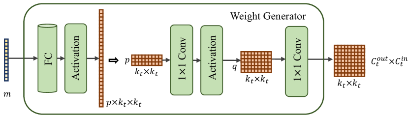
Figure 4: Architecture of the weight generator.

When the parameters of each layer in the target network are predicted, we can use these predicted parameters as the final parameters of $\Omega$ for inference.

III-E Optimization of Our Framework

In this section, we introduce how to optimize our PudNet. In contrast to traditional classification tasks where training data and testing data have the identical label space. In our task, the label spaces between training and testing can be different, even not overlapped. Thus, training a classification head on training data can not be used to predict labels of testing data. Motivated by several metric learning methods [44, 53], we introduce a parameter-free classification method to solve the above issue.

Similar to [44], we obtain a metric-based category prediction on class $c_{k}$ as:

$$p(y=c_{k}|x_{j},\Omega,D_{i};H_{\theta})$$

$$=\frac{exp(\tau\cdot<f(x_{j};\mathcal{F}(D_{i},\Omega;H_{\theta})),\mathbf{u}_{k}>)}{\sum_{c}{exp}(\tau\cdot<f(x_{j};\mathcal{F}(D_{i},\Omega;H_{\theta})),\mathbf{u}_{c}>)},$$ (7)

where $\mathbf{u}_{k}$ is the centroid of class $c_{k}$, which is the average output of the predicted network $\Omega$ over samples belonging to class $c_{k}$, as in [40]. $<\cdot,\cdot>$ denotes the cosine similarity of two vectors, and $\tau$ is a learnable temperature parameter. $f(x_{j};\mathcal{F}(D_{i},\Omega;H_{\theta}))$ is the output of the target network $\Omega$ based on the input $x_{j}$. Then, the parameter-free classification loss can be defined as:

$$\mathcal{L}_{1}=\sum_{i=1}^{\mathcal{N}}\sum_{x_{j}\in D_{i}}\mathcal{L}(p(y|x_{j},\Omega,D_{i};H_{\theta}),y_{j}),$$ (8)

where $y_{j}$ is the true label of $x_{j}$, $\mathcal{L}$ is the cross-entropy loss.

To further improve the performance of the model, we add a full classification head $\mathcal{Q}_{\varphi}$ parameterized by $\varphi$ as an auxiliary task for training our hypernetwork, motivated by [53]. The classification head aims to map the output of the target network $\Omega$ to probabilities of the whole classes $\mathcal{C}^{tr}$ from $\mathcal{D}^{train}$. The full classification loss is defined as:

$$\mathcal{L}_{2}=\sum_{i=1}^{\mathcal{N}}\sum_{x_{j}\in D_{i}}\mathcal{L}(\mathcal{Q_{\varphi}}(f(x_{j};\mathcal{F}(D_{i},\Omega;H_{\theta}))),y_{j}).$$ (9)

Moreover, to make parameter-free based prediction and full classification based prediction consistent, which is motivated by [54, 55], we introduce a Kullback-Leibler Divergence loss to encourage their predicted probabilities to be matched:

$$\mathcal{L}_{3}=\sum_{i=1}^{\mathcal{N}}\sum_{x_{j}\in D_{i}}KL(q(y|x_{j})||p(y|x_{j})),$$ (10)

where $KL$ is the Kullback-Leibler Divergence. $p(y|x_{j})$ and $q(y|x_{j})$ are the predicted probabilities of $x_{j}$ of parameter-free based and full classification based methods, respectively. The probabilities of corresponding classes in $p(y|x_{j})$ are padding with zero to match the dimension of $q(y|x_{j})$.

Finally, we give the overall multi-task loss as:

$$\mathcal{L}_{train}=\mathcal{L}_{1}+\mathcal{L}_{2}+\mathcal{L}_{3}.$$ (11)

where $D_{i}$ can be regarded as a task similar to that in meta-learning. By minimizing (11), our hypernetwork can be well trained. For an unseen data in testing, we utilize our hypernetwork to directly predict its network parameters, and use the parameter-free based method for classification.

We provide the training procedure of our PudNet as listed in Algorithm 1. For each training dataset $D_{i}\in\mathcal{D}^{train}$, we first derive the sketch $\mathbf{s}_{i}$ of dataset $D_{i}$ and set the initial hidden state $\mathbf{d}_{0}^{(i)}=\mathbf{s}_{i}$ in AHRU. Then, we predict the parameters of each layer in the target network $\Omega$. Finally, we optimize the the learnable parameters $\theta$, $\varphi$ by the the overall multi-task loss $\mathcal{L}_{train}$. We also present the inference process of our PudNet for an unseen dataset, as listed in Algorithm 2.

Input: A set of training datasets $\mathcal{D}^{train}=\{D_{i}\}_{i=1}^{\mathcal{N}}$, target network architecture $\Omega$.

1   Initialize the learnable parameter $\theta$ of $H_{\theta}$.

2   Initialize the learnable parameter $\varphi$ of the auxiliary full classification.

3 while not converged do

4       for  $i\in\{1,\cdots,\mathcal{N}\}$  do

5               Obtain a sketch $\mathbf{s}_{i}$ of dataset $D_{i}$ via the dataset compression module;

6               Initialize the hidden state $\mathbf{d}_{0}^{(i)}=\mathbf{s}_{i}$;

7             for  each layer $t$ in $\Omega$ do

8                   Predict the parameters $w_{t}^{(i)}$ of the $t$-th layer by weight generator;

9                   Fix the predicted parameters $w_{t}^{(i)}$ to $\Omega$;

10             end for

11            for  each batch $b$ in $D_{i}$ do

12                   Compute the parameter-free loss $\mathcal{L}_{1}$ with a batch size of $b$;

13                   Compute the full classification loss $\mathcal{L}_{2}$ and consistency loss $\mathcal{L}_{3}$ with a batch size of $b$;

14                   Update the learnable parameters $\theta$, $\varphi$ by the overall multi-task loss $\mathcal{L}_{train}$ ;

15             end for

16            

17       end for

18      

19 end while

Output: The PudNet $H_{\theta}$.

Algorithm 1 The Training of PudNet

Input: An unseen dataset $D_{i}\in\mathcal{D}^{test}$, the learned PudNet $H_{\theta}$, target network architecture $\Omega$.

1 for  each layer $t$ in $\Omega$ do

2         Predict the parameters $w_{t}^{(i)}$ of the $t$-th layer by the PudNet $H_{\theta}$;

3         Fix the predicted parameters $w_{t}^{(i)}$ to $\Omega$;

4 end for

5  Conduct inference for dataset $D_{i}$ with parameterized network $\Omega$ ;

Output: The prediction results for dataset $D_{i}$.

Algorithm 2 The Inference of PudNet for Unseen Data

III-F Theoretical Analysis of the Hyper-Mapping

We provide a theoretical analysis of how the model learns hyper-mapping between datasets and their corresponding network parameters, which offers interpretability.

Recall that for each image dataset $D_{i}\in\mathcal{D}^{train}$, the learning of the hyper-mapping between dataset $D_{i}$ and their corresponding network parameters $\mathcal{M}_{i}$ can be formulated as: leveraging a hyper-network $H_{\theta}$ to produce an optimal model $\Omega_{\mathcal{M}_{i}^{*}}$ with parameters $\mathcal{M}_{i}^{*}=H_{\theta}(D_{i})$ via optimizing $\mathop{\arg\min}\limits_{\theta}\sum_{D_{i}\in\mathcal{D}^{train}}\mathcal{L}(\Omega_{\mathcal{M}_{i}^{*}},D_{i})$. To write conveniently, here we denote $D_{i}$ as $d$. We can learn the hypernetwork $H_{\theta}$ by solving an optimization problem:

$$\mathop{\arg\min}\limits_{\theta}\mathbb{E}_{d\sim p(d)}\mathcal{L}(H_{\theta}(d),d).$$

It is generally feasible to solve $H_{\theta}$. We use $h$ to represent $H_{\theta}$ and instead optimize the problem with the form $h^{*}:=\mathop{\arg\min}_{h}\mathcal{L}(h(d),d)$. For $h$, conditioning $\mathcal{L}(h^{*}(d),d)$ is an extremum for any infinitesimal $\delta d$, we can deduce $h^{*}$ using the ordinary differential equation:

$$\frac{\partial\mathcal{L}}{\partial{h}}(h^{*}(d+\delta d),d+\delta d)=\frac{\partial^{2}\mathcal{L}}{\partial h^{2}}\frac{\partial h^{*}}{\partial d}\delta d+\frac{\partial^{2}\mathcal{L}}{\partial h\partial d}\delta d+O(\delta d)=0.$$

Then we can get:

$$\frac{\partial^{2}\mathcal{L}}{\partial h^{2}}\frac{\partial h^{*}}{\partial d}=-\frac{\partial^{2}\mathcal{L}}{\partial h\partial d}.$$ (12)

We step further by utilizing the product rule and chain rule to compute the derivative $\frac{\partial h^{*}}{\partial d}$ and substitute $\frac{\partial\mathcal{L}}{\partial h}=\frac{\partial\mathcal{L}}{\partial y}\frac{\partial y}{\partial h}$ into the equation, where $y$ is the output of the ConvNet model. Given these, $\frac{\partial^{2}\mathcal{L}}{\partial h^{2}}$ is the Hessian matrix of $\mathcal{L}$ with respect to $h$ as:

$$\frac{\partial^{2}\mathcal{L}}{\partial{{h^{2}}}}=\frac{\partial^{2}\mathcal{L}}{\partial y^{2}}(\frac{\partial y}{\partial h})^{2}+\frac{\partial\mathcal{L}}{\partial{y}}\frac{\partial^{2}y}{\partial{h^{2}}},$$ (13)

and we have:

$$\frac{\partial^{2}\mathcal{L}}{\partial{{h}}\partial{{d}}}= (\frac{\partial^{2}\mathcal{L}}{\partial y^{2}}\frac{\partial y}{\partial d}+\frac{\partial^{2}\mathcal{L}}{\partial y^{2}}\frac{\partial y}{\partial h}\frac{\partial h}{\partial d})\frac{\partial y}{\partial h}$$

$$+\frac{\partial\mathcal{L}}{\partial y}(\frac{\partial^{2}y}{\partial h\partial d}+\frac{\partial^{2}y}{\partial{h^{2}}}\frac{\partial h}{\partial d})$$ (14)

Assuming that the Hessian of $\mathcal{L}$ is non-singular, thus we can solve for $\frac{\partial h^{*}}{\partial d}$ as:

$$\frac{\partial h^{*}}{\partial d}=-\frac{1}{2}(\frac{\partial^{2}\mathcal{L}}{\partial{{y^{2}}}}(\frac{\partial{y}}{\partial{h}})^{2}+\frac{\partial\mathcal{L}}{\partial{y}}\frac{\partial^{2}y}{\partial{h^{2}}})^{-1}(\frac{\partial^{2}\mathcal{L}}{\partial{y^{2}}}\frac{\partial y}{\partial d}\frac{\partial y}{\partial h}+\frac{\partial\mathcal{L}}{\partial y}\frac{\partial^{2}y}{\partial h\partial d}),$$

where the superscript ${-1}$ denotes the matrix inversion.

Suppose we have found a solution $h^{*}$ of the optimization problem $\mathop{\arg\min}_{h^{*}}\mathcal{L}(h^{*},d_{0})$ for the dataset $d=d_{0}$. We want to use this solution to ”track” the local minimum of the loss $\mathcal{L}$ as we move from $d_{0}$ to another dataset $d=d_{1}$ in a small vicinity of $d_{0}$, where the loss $\mathcal{L}$ remains convex and the Hessian of the loss $\mathcal{L}$ is not singular.

To do this, we can use an ordinary differential equation (ODE) approach to integrate the solution with respect to a path $\hat{d}$ that connects the two datasets $d_{0}$ and $d_{1}$. To track the local minimum of the loss function as we move from $d_{0}$ to $d_{1}$ along the path $\hat{d}$, we need to integrate the above path $\hat{d}$ with $\partial h^{*}/\partial d$ as the derivative, where $d_{0}=\hat{d}(0)$ and $d_{1}=\hat{d}(1)$. By solving this ODE numerically, we obtain the solution that corresponds to the local minimum of the loss $\mathcal{L}$:

$$\frac{d{h^{*}}}{d\gamma} =\frac{\partial h^{*}}{\partial\hat{d}}\frac{d\hat{d}}{d\gamma}$$

$$= -\frac{1}{2}(\frac{\partial^{2}\mathcal{L}}{\partial{{y^{2}}}}(\frac{\partial{y}}{\partial{h}})^{2}+\frac{\partial\mathcal{L}}{\partial{y}}\frac{\partial^{2}y}{\partial{h^{2}}})^{-1}\frac{\partial^{2}\mathcal{L}}{\partial{y^{2}}}\frac{\partial y}{\partial\hat{d}}\frac{\partial y}{\partial h}\frac{d\hat{d}}{d\gamma}$$

$$-\frac{1}{2}(\frac{\partial^{2}\mathcal{L}}{\partial{{y^{2}}}}(\frac{\partial{y}}{\partial{h}})^{2}+\frac{\partial\mathcal{L}}{\partial{y}}\frac{\partial^{2}y}{\partial{h^{2}}})^{-1}\frac{\partial\mathcal{L}}{\partial y}\frac{\partial^{2}y}{\partial h\partial\hat{d}}\frac{d\hat{d}}{d\gamma},$$ (15)

where $\gamma$ changes from 0 to 1, and all derivatives are computed at $\hat{d}(\gamma)$ and $h^{*}(\gamma)$.

So far, the above equation gives us the way to get the empirical solution of $H_{\theta}$ directly with respect to the proposed PudNet. These aforementioned concepts provide a theoretical basis and the interpretability of hyper-mapping learning between datasets and their corresponding network parameters.

IV Experiment

IV-A Dataset Construction

In the experiment, we construct numerous datasets for evaluating our method based on several image datasets: Fashion-MNIST [14], CIFAR-100 [15], Mini-ImageNet [16], Animals-10 [56], CIFAR-10 [15], DTD [57], and a large-scale dataset, ImageNet-1K  [5]. The constructed datasets are based on two following settings: Intra-dataset prediction setting and Inter-dataset prediction setting.

The intra-dataset prediction setting is described as follows:

Fashion-set: We construct 2000 groups of datasets from the samples of 6 classes on Fashion-MNIST to train PudNet. The testing groups of datasets are constructed from samples of the remaining 4 classes. we construct 500 groups of datasets from the 4-category testing set to generate 500 groups of network parameters. For each group of network parameters, we also construct another dataset having identical labels but not having overlapped samples with the dataset used for generating parameters, in order to test the performance of the predicted network parameters.

CIFAR-100-set: We choose 80 classes from CIFAR-100 for training sets and 20 not overlapped classes for testing sets. We sample 100000 groups of datasets for training. Similar to Fashion-set, we construct 500 groups of datasets for parameter prediction, and another 500 groups for testing.

ImageNet-100-set: Similar to CIFAR-100-set, we sample 50000 groups of datasets from 80-category training sets of Mini-ImageNet to train PudNet. We construct 500 groups of datasets from remaining 20-category testing sets to predict parameters, and sample another 500 groups for testing.

ImageNet-1K-set: We partition ImageNet-1K into mutually exclusive sets of 800 classes for training and 200 classes for testing. For the training set of 800 classes, we construct 20000 sub-datasets to train PudNet. We employ the testing data of 200 classes to evaluate the performance of PudNet.

Note that the training class set and testing class set in the above datasets are not overlapped.

To further verify our PudNet, we introduce an inter-dataset setting by constructing cross-domain datasets. We construct three training datasets: CIFAR-100-set with 100000 dataset groups, ImageNet-100-set with 50000 dataset groups, and ImageNet-1K-set with 20000 dataset groups. Each of these datasets is used individually to train PudNet. The samples in Animals-10, CIFAR-10, and DTD are used for evaluation, respectively. Note that ImageNet and the above three other datasets are popular cross-domain datasets, which have been widely used for out-of-distribution (OOD) learning [58, 59], and cross-domain learning [60, 61]. The constructed datasets are summarized as follows:

CIFAR-100$\to$Animals-10, ImageNet-100$\to$Animals-10, ImageNet-1k$\to$Animals-10: We randomly select 80% of the samples from Animals-10 and feed them into PudNet, which is trained on CIFAR-100-set, ImageNet-100-set, and ImageNet-1K-set, respectively, in order to generate network parameters. The remaining 20% of samples are then used to test the performance of the predicted network parameters.

CIFAR-100$\to$CIFAR-10, ImageNet-100$\to$CIFAR-10, ImageNet-1k$\to$CIFAR-10: We randomly select 50000 samples in CIFAR-10 to feed into the PudNet, trained on CIFAR-100-set, ImageNet-100-set and ImageNet-1K-set respectively, so as to generate network parameters, and use the rest 10000 samples for testing.

CIFAR-100$\to$DTD, ImageNet-100$\to$DTD, ImageNet-1k$\to$DTD: DTD is an image texture classification dataset [57], which is integrated into the visual adaptation benchmark [62]. The labels of DTD are very different from those of ImageNet. We randomly choose 2/3 samples from DTD to generate parameters and the rest for testing.

TABLE I: Results of different methods in terms of the target network ResNet-18 in the intra-dataset setting.

Method		Fashion-set		CIFAR-100-set		ImageNet-100-set
		ACC(%)	time (sec.)	ACC	time (sec.)	ACC	time (sec.)
Pretrained		93.76$\pm$0.47	-	64.58$\pm$0.59	-	65.67$\pm$0.73	-
MatchNet [16]		90.16$\pm$0.53	-	56.23$\pm$0.71	-	53.17$\pm$0.91	-
ProtoNet [40]		93.64$\pm$0.47	-	60.29$\pm$0.59	-	58.95$\pm$0.83	-
Meta-Baseline [44]		95.35$\pm$0.29	-	67.51$\pm$0.55	-	67.16$\pm$0.70	-
Meta-DeepDBC [45]		94.28$\pm$0.31	-	69.54$\pm$0.49	-	68.48$\pm$0.60	-
MUSML [43]		95.87$\pm$0.44	2.55	66.47$\pm$0.63	2.59	66.03$\pm$0.91	2.60
Adam Scratch [6]	1 epoch	93.98$\pm$1.21	1.83	52.82$\pm$1.01	3.96	46.43$\pm$1.18	4.81
	30 epochs	99.91$\pm$0.05	54.22	74.56$\pm$0.45	118.87	71.84$\pm$0.69	140.37
	50 epochs	99.87$\pm$0.11	91.19	79.85$\pm$0.47	198.12	75.98$\pm$0.71	231.63
GC Scratch [9]	1 epoch	94.11$\pm$1.25	1.88	53.21$\pm$1.23	4.01	47.55$\pm$1.33	4.82
	30 epochs	99.94$\pm$0.05	54.93	75.74$\pm$0.59	119.03	72.89$\pm$0.73	140.98
	50 epochs	99.96$\pm$0.03	91.73	79.98$\pm$0.55	199.61	76.73$\pm$0.87	232.57
PudNet		96.24$\pm$0.39	0.50	73.33$\pm$0.54	0.49	71.57$\pm$0.71	0.50

TABLE II: Results of different methods in terms of the target network ResNet-18 in the inter-dataset setting.

Method		CIFAR-100$\to$Animals-10		CIFAR-100$\to$CIFAR-10		CIFAR-100$\to$DTD
		ACC (%)	time (sec.)	ACC (%)	time (sec.)	ACC (%)	time (sec.)
Pretrained		33.36$\pm$0.75	-	40.93$\pm$0.48	-	30.27±0.58	-
MatchNet [16]		33.08$\pm$0.70	-	39.82$\pm$0.69	-	27.17$\pm$0.73	-
ProtoNet [40]		36.33$\pm$0.60	-	43.22$\pm$0.54	-	32.66$\pm$0.63	-
Meta-Baseline [44]		38.27$\pm$0.53	-	45.43$\pm$0.59	-	34.25$\pm$0.58	-
Meta-DeepDBC [45]		40.50$\pm$0.64	-	47.15$\pm$0.63	-	35.50$\pm$0.71	-
MUSML [43]		37.78$\pm$0.59	3.21	45.37$\pm$0.57	5.34	33.34±0.68	2.18
Adam Scratch [6]	1 epoch	22.09$\pm$0.58	31.29	21.37$\pm$0.71	60.79	18.83$\pm$0.19	4.03
	5 epochs	49.12$\pm$0.08	156.56	33.76$\pm$0.44	310.29	24.17$\pm$0.72	26.01
	10 epochs	66.44$\pm$0.37	311.74	48.21$\pm$0.25	621.75	33.26$\pm$0.90	51.79
	20 epochs	73.47$\pm$0.67	623.92	65.17$\pm$0.55	1248.23	42.51$\pm$0.44	102.11
	50 epochs	77.81$\pm$0.34	1558.51	80.25$\pm$0.61	3109.87	52.16$\pm$0.56	257.91
GC Scratch [9]	1 epoch	23.01$\pm$1.02	30.79	21.44$\pm$1.02	60.99	18.67$\pm$0.34	4.01
	5 epochs	49.77$\pm$0.54	155.34	34.41$\pm$0.78	310.33	24.43$\pm$0.83	25.87
	10 epochs	68.56$\pm$0.39	310.29	49.89$\pm$0.53	622.01	35.49$\pm$0.61	51.70
	20 epochs	75.04$\pm$0.61	623.33	66.78$\pm$0.47	1248.98	44.05±0.52	102.63
	50 epochs	77.98$\pm$0.45	1557.76	82.03$\pm$0.42	3109.14	53.58±0.61	257.24
PudNet		43.21$\pm$0.69	0.49	51.05$\pm$0.56	0.56	38.05$\pm$0.73	0.39

IV-B Baselines and Implementation Details

We compare our method with the most related work, i.e., traditional iterative based training paradigm including training from scratch with Adam [6] and one training acceleration method, GC [9]. We also take the pretrained model as a baseline. In addition, we compare with meta-learning methods, including MatchNet [16], ProtoNet [40], Meta-Baseline [44], Meta-DeepDBC [45], and MUSML [43]. We use three kinds of architectures as our target network $\Omega$ respectively: a 3-layer CNN ConvNet-3, ResNet-18[4], ResNet-34[4]. Throughout the experiments, we use the accuracy (ACC) metric to evaluate the classification performance. We employ Top-1 Accuracy as the evaluation metric, unless otherwise specified.

We perform the experiments using GeForce RTX 3090 Ti GPU. All experiments are optimized by the Adam optimizer. We set the learning rate to 0.001 and train PudNet until convergence. In metric-based learning process, following [44], the temperature $\tau=10$ in Eq.(7) is fixed. 10 labeled samples per class are used to deduce the class centroid. As mentioned before, we introduce auxiliary tasks to assist optimization. We add a full classification linear layer (e.g. 80-way linear head in CIFAR-100) to maintain static class set during training. We also introduce a consistency loss, since the dimension between logits deduced by metric-based classification (e.g.5-dimensional in CIFAR-100) and the logits produced by full linear head (e.g.80-dimensional in CIFAR-100) are not matched, we transpose the 5-dimensional logit to 80-dimensional logit, by padding the rest values with zero. We search $\eta$ from $\{0,0.1,0.2,0.3,\cdots,0.9\}$. For the target network ResNet-18, we set $\eta=0.2$ for Fashion-set, $\eta=0.5$ for CIFAR-100-set, ImageNet-100-set and ImageNet-1K-set. The hyperparameter $\eta$ is set as 0.5 on the inter-dataset setting datasets. For the target network ConvNet-3, we set $\eta=0.1$, and for the target network ResNet-34, we set $\eta=0.5$.

IV-C Result and Analysis

Performance Analysis of Intra-dataset Prediction. Table I shows the results of our method in the intra-dataset setting. We could find that our method consistently outperforms the meta-learning methods and the pretrained method. This demonstrates that learning a hyper-mapping between datasets and corresponding network parameters is effective. To demonstrate the time consumption our method could save, we also provide the time of training the model from scratch by a widely-used optimizer Adam and the training acceleration technique, GC. We find that it takes around 55, 119, 141 GPU seconds to train ResNet-18 using the accelerated method GC and the network obtains top-1 accuracies of 99.94%, 75.74%, 72.89% on Fashion-set, CIFAR-100-set, ImageNet-100-set respectively. While our method costs only around 0.5 GPU seconds to predict the parameters of ResNet-18 and still achieves a comparable performance (96.24%, 73.33%, 71.57% top-1 accuracies) on the three datasets respectively, at least 100 times faster than the accelerated method.

TABLE III: Results of different methods in terms of the target network ResNet-18 in the inter-dataset setting.

Method		ImageNet-100$\to$Animals-10		ImageNet-100$\to$CIFAR-10		ImageNet-100$\to$DTD
		ACC (%)	time (sec.)	ACC (%)	time (sec.)	ACC (%)	time (sec.)
Pretrained		34.79$\pm$0.49	-	34.54$\pm$0.63	-	31.05$\pm$0.51	-
MatchNet [16]		32.38$\pm$0.82	-	31.98$\pm$0.72	-	28.15$\pm$0.67	-
ProtoNet [40]		35.78$\pm$0.64	-	35.21$\pm$0.74	-	31.58$\pm$0.77	-
Meta-Baseline [44]		36.21$\pm$0.42	-	38.34$\pm$0.69	-	33.07$\pm$0.83	-
Meta-DeepDBC [45]		38.57$\pm$0.55	-	40.93$\pm$0.71	-	34.01$\pm$0.69	-
MUSML [43]		36.89$\pm$0.44	3.21	37.12$\pm$0.65	5.34	33.67$\pm$0.63	2.18
Adam Scratch [6]	1 epoch	22.09$\pm$0.58	31.29	21.37$\pm$0.71	60.79	18.83$\pm$0.19	4.03
	5 epochs	49.12$\pm$0.08	156.56	33.76$\pm$0.44	310.79	24.17$\pm$0.72	26.01
	10 epochs	66.44$\pm$0.37	311.74	48.21$\pm$0.25	621.75	33.26$\pm$0.90	51.79
	20 epochs	73.47$\pm$0.67	623.92	65.17$\pm$0.55	1248.23	42.51$\pm$0.44	102.11
	50 epochs	77.81$\pm$0.34	1558.51	80.25$\pm$0.61	3109.87	52.16$\pm$0.56	257.91
GC Scratch [9]	1 epoch	23.01$\pm$1.02	30.79	21.44$\pm$1.02	60.99	18.67$\pm$0.34	4.01
	5 epochs	49.77$\pm$0.54	155.34	34.41$\pm$0.78	310.33	24.43$\pm$0.83	25.87
	10 epochs	68.56$\pm$0.39	310.29	49.89$\pm$0.53	622.01	35.49$\pm$0.61	51.70
	20 epochs	75.04$\pm$0.61	623.33	66.78$\pm$0.47	1248.98	44.05$\pm$0.52	102.63
	50 epochs	77.98$\pm$0.45	1557.76	82.03$\pm$0.42	3109.14	53.58$\pm$0.61	257.24
PudNet		42.43$\pm$0.58	0.48	45.07$\pm$0.70	0.57	47.50$\pm$0.71	0.39

TABLE IV: Results of different methods on ImageNet-1K-set in the intra-dataset setting.

Method		ImageNet-1K-set
		ACC(%)	time(sec.)
Pretrained		35.77$\pm$0.84	-
Meta-Baseline		38.92$\pm$0.93	-
Meta-DeepDBC		39.15$\pm$1.12	-
MUSML		41.33$\pm$0.95	35.17
	100 steps	9.35 $\pm$1.42	229.33
GC	2000 steps	37.48$\pm$0.81	4488.71
Scratch	4000 steps	44.65$\pm$0.97	8967.55
[9]	6000 steps	52.03$\pm$0.85	13453.29
PudNet		44.92$\pm$0.91	3.89

TABLE V: Results of different methods on ImageNet-1K in the inter-dataset setting.

Method		ImageNet-1K$\to$Animals-10		ImageNet-1K$\to$CIFAR-10		ImageNet-1K$\to$DTD
		ACC (%)	time (sec.)	ACC (%)	time (sec.)	ACC (%)	time (sec.)
Pretrained		51.02$\pm$0.54	-	40.31$\pm$0.69	-	44.19$\pm$0.61	-
Meta-Baseline [44]		52.19$\pm$0.63	-	42.66$\pm$0.72	-	45.43$\pm$0.89	-
Meta-DeepDBC [45]		54.37$\pm$0.59	-	44.74$\pm$0.70	-	46.53$\pm$0.72	-
MUSML [43]		53.81$\pm$0.58	4.08	44.23$\pm$0.74	6.07	45.92$\pm$0.76	2.91
GC Scratch [9]	1 epoch	23.01$\pm$1.02	30.79	21.44$\pm$1.02	60.99	18.67$\pm$0.34	4.01
	5 epochs	49.77$\pm$0.54	155.34	34.41$\pm$0.78	310.33	24.43$\pm$0.83	25.87
	10 epochs	68.56$\pm$0.39	310.29	49.89$\pm$0.53	622.01	35.49$\pm$0.61	51.70
	20 epochs	75.04$\pm$0.61	623.33	66.78$\pm$0.47	1248.98	44.05$\pm$0.52	102.63
	50 epochs	77.98$\pm$0.45	1557.76	82.03$\pm$0.42	3109.14	53.58$\pm$0.61	257.24
PudNet		58.51$\pm$0.63	0.51	51.03$\pm$0.68	0.63	54.50$\pm$0.74	0.32

Performance Analysis of Inter-dataset Prediction. We further evaluate our method in the inter-dataset setting. The results are listed in Table II and Table III, which shows the efficiency of our PudNet. For instance, as shown in Table III on the ImageNet-100$\to$CIFAR-10 dataset, our PudNet can achieve comparable top-1 accuracy with that of training the model from scratch on CIFAR-10 at around 10 epochs, while PudNet is at least 1000 times faster than traditional training methods, Adam and GC. Besides, our model still outperforms meta-learning methods in a large margin. More surprisingly, although the label space of DTD (a texture classification dataset) is significantly different from that of ImageNet-100, our method still obtains good efficacy. We expect that such results can motivate more researchers to explore along this direction.

Scaling Up to ImageNet-1K. For the intra-dataset setting, we partition ImageNet-1K into mutually exclusive sets of 800 classes for training and 200 classes for testing. Top-5 accuracies of different methods are reported as in Table IV. We can observe that our method still achieves surprisingly good efficiency. For instance, It takes 8967 GPU seconds to train ResNet-18 on the ImageNet-1K using GC from scratch and obtain a top-5 accuracy of 44.65 %. However, our PudNet costs only 3.89 GPU seconds to predict the network parameters of ResNet-18 achieving comparable performance (44.92 %), more than 2,300 times faster than the traditional training paradigm. In addition, our method also outperforms the state-of-the-art meta-learning methods in a large margin. These show that PudNet can effectively scale to a larger and more complex dataset.

For the inter-dataset setting, we add another experiments on three inter-datasets: ImageNet-1K $\to$ Animals-10, ImageNet-1K $\to$ CIFAR-10 and ImageNet-1K $\to$ DTD. The results are listed as in Table V. Based on the above table, our method still achieves surprisingly good efficiency. Please kindly note that compared to our PudNet trained on ImageNet-100, as in Table III, which achieves 42.43 % top-1 accuracy on Animals-10, 45.07% top-1 accuracy on CIFAR-10, and 47.5% top-1 accuracy on DTD, training PudNet on the larger ImageNet dataset yields an improvement of approximately 16%, 6%, and 7% on the three inter-dataset tasks, respectively, while requiring comparable time costs. This indicates that training our model with more complex and comprehensive datasets results in better generalization performance. Based on the experiments on both intra-dataset and inter-dataset settings, our PudNet can effectively scale to larger datasets.

Ablation Study. We design several variants of our method to analyse the effect of different parts in both intra-dataset and inter-dataset settings. We first analyse the effect of the context relation information. The results are listed in Table VI. PudNet-w.o.-Context denotes our method directly feeds the dataset sketch into the weight generator without using AHRU. Our PudNet outperforms PudNet-w.o.-Context in a large margin, demonstrating the effectiveness of capturing dependencies among parameters of different layers.

We further evaluate the effect of the auxiliary task. PudNet-metric means our method only uses the parameter-free loss. PudNet-w.o.-kl means our method does not use the KL Divergence. As shown in Table VI, PudNet-w.o.-kl has better performance than PudNet-metric, demonstrating the effectiveness of the auxiliary full classification task. PudNet outperforms PudNet-w.o.-kl, illustrating the effectiveness of matching the predicted probability distributions of the parameter-free method and full classification method.

Performance Analysis of Different Target Networks. We conduct experiments to further evaluate our method by predicting parameters of different target network architectures: ConvNet-3 and ResNet-34. The results are listed in Table VII. We observe that our method can obtain comparable top-1 accuracy to those of GC at 30 epochs for different target network architectures, while our method is more than 250 times faster than GC. This further demonstrates the efficiency of our method.

TABLE VI: Ablation study of our method PudNet. ‘IN’ denotes ‘ImageNet-100’.

Method	Intra-dataset			Inter-dataset
	Fashion-set	CIFAR-100-set	ImageNet-100-set	IN$\to$Animals-10	IN$\to$CIFAR-10	IN$\to$DTD
PudNet-w.o.-Context	93.08$\pm$0.44	65.35$\pm$0.51	61.42$\pm$0.70	37.21$\pm$0.51	39.43$\pm$0.68	37.79$\pm$0.83
PudNet-metric	94.75$\pm$0.44	68.60$\pm$0.61	61.28$\pm$0.85	40.35$\pm$0.60	43.78$\pm$0.69	43.67$\pm$0.72
PudNet-w.o.-kl	95.44$\pm$0.38	70.27$\pm$0.54	67.53$\pm$0.73	41.23$\pm$0.68	43.98$\pm$0.74	45.12$\pm$0.88
PudNet	96.24$\pm$0.39	73.33$\pm$0.54	71.57$\pm$0.71	42.43$\pm$0.58	45.07$\pm$0.70	47.50$\pm$0.71

TABLE VII: Results of different methods in terms of different target network architectures on CIFAR-100-set.

		ConvNet-3		ResNet-34
Method		ACC(%)	time(sec.)	ACC(%)	time(sec.)
Pretrained		58.35$\pm$0.61	-	65.03$\pm$0.53	-
MatchNet		47.75$\pm$0.73	-	60.37$\pm$0.70	-
ProtoNet		51.96$\pm$0.57	-	64.28$\pm$0.58	-
Meta-baseline		57.69$\pm$0.38	-	67.40$\pm$0.69	-
Meta-DeepDBC		60.52$\pm$0.41	-	69.64$\pm$0.75	-
MUSML		56.49$\pm$0.56	1.21	66.39$\pm$0.59	3.11
Adam Scratch	1 epoch	49.11$\pm$1.03	0.99	47.39$\pm$1.36	5.47
	30 epochs	64.54$\pm$0.40	28.37	71.17$\pm$0.53	153.87
	50 epochs	70.68$\pm$0.53	49.02	78.72$\pm$0.71	263.25
GC Scratch	1 epoch	50.23$\pm$1.23	0.99	48.44$\pm$1.41	5.52
	30 epochs	66.76$\pm$0.54	29.8	72.37$\pm$0.75	154.19
	50 epochs	71.56$\pm$0.63	50.2	79.85$\pm$0.83	264.03
PudNet		64.09$\pm$0.40	0.03	72.87$\pm$0.64	0.59

Finetuning Predicted Parameters. Since a typical strategy for applying a pretrained model to a new dataset is to finetune the model, we evaluate our method by finetuning the models obtained by the intra-dataset, CIFAR-100-set, and the inter-dataset, ImageNet-100$\to$DTD. We first incorporate an additional linear classification layer to our method and baselines, except ‘Adam Scratch’ and ’GC Scratch’. Then, we randomly select 10000 images from CIFAR-100 and 800 images from DTD to finetune the models, respectively. The remaining images are used for testing, respectively. Table VIII shows the results. Our method achieves the best performance. This indicates that the predicted parameters by our PudNet can well serve as a pretrained model.

TABLE VIII: Performance of finetuning all methods on target network ResNet-18 using 50 epochs.

Method	CIFAR-100-set	ImageNet-100$\to$DTD
Pretrained	59.75$\pm$0.24	53.43$\pm$0.43
MatchNet	56.83$\pm$0.40	52.26$\pm$0.71
ProtoNet	58.14$\pm$0.29	54.44$\pm$0.64
Meta-baseline	60.05$\pm$0.27	54.52$\pm$0.58
Meta-DeepDBC	61.35$\pm$0.28	55.09$\pm$0.63
MUSML	59.28$\pm$0.29	53.61$\pm$0.69
Adam Scratch	48.25$\pm$0.30	52.16$\pm$0.56
GC Scratch	50.03$\pm$0.32	53.58$\pm$0.61
PudNet	65.19$\pm$0.22	58.25$\pm$0.57

Effect of Different Groups of Datasets. We analyze the effect of different groups of datasets for training. Fig. 5 reports the results of exploiting PudNet to predict parameters for ResNet-18. We construct varying groups of datasets for training our PudNet on Fashion-set, CIFAR-100-set, ImageNet-100-set respectively. We find that with more groups of datasets for training, our PudNet could obtain better performance. This is because with larger number of groups to learn the hyper-mapping relation, our PudNet could obtain better generalization ability. However, when the number of groups becomes large, the performance increase becomes slow.

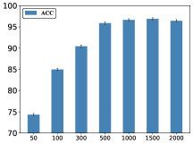
(a) Fashion-set

(b) CIFAR-100-set

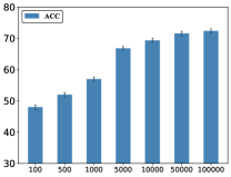
(c) ImageNet-100-set

Figure 5: Effect of different groups of datasets in terms of the target network ResNet-18.

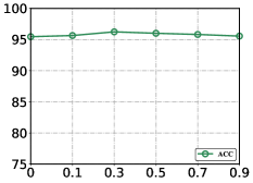
(a) Fashion-set with ResNet-18

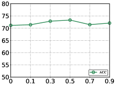
(b) ​CIFAR-100-set​ with ResNet-18​

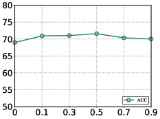
(c) ImageNet-100-set with ResNet-18

Figure 6: Sensitivity analysis of hyper-parameter $\eta$.

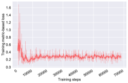
(a) metric loss on Fashion-set

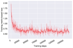
(b) metric loss on CIFAR-100-set

(c) metric loss on ImageNet-100-set

(d) total training loss on Fashion-set

(e) total training loss on CIFAR-100-set

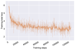
(f) total training loss on ImageNet-100-set

Figure 7: Training loss of PudNet.

Parameter Sensitive Analysis. We analyze the effect of different values of the hyper-parameter $\eta$. Recall that $\eta$ controls the percent of dataset complementary information in the initial residual connection. Fig. 6(a)(b)(c) show the results in terms of ResNet-18. We observe that our model obtain better performance when $\eta>0$ in general. Additionally, our method is not sensitive to $\eta$ in a relatively large range.

Convergence Analysis. We discuss the convergence property of the proposed method by plotting the loss curves with increasing iteration. Here we utilize PudNet to predict parameters for ResNet-18, based on Fashion-set, CIFAR-100-set and ImageNet-100-set respectively. As shown in Fig. 7, the training metric-based loss (abbreviated as metric loss) and training total loss first decrease rapidly as the number of iterations increases, and then gradually decrease to convergence.

V Conclusion and Limitations

In this paper, we found there are correlations among image datasets and the corresponding parameters of a given ConvNet, and explored a new training paradigm for ConvNets. We proposed a new hypernetwork, called PudNet, which could directly predict the network parameters for an image unseen dataset with only a single forward propagation. In addition, we attempted to capture the relations among parameters of different layers in a network by a series of adaptive hyper recurrent units. Extensive experimental results demonstrated the effectiveness and efficiency of our method on both intra-dataset prediction setting and inter-dataset prediction setting. However, current work primarily focused on exploring the generation of parameters for the target networks based on CNNs. A potential avenue for future research could involve extending parameter generation to other target network architectures, e.g., large language models.

Shiye Wang received the M.S. degree in computer science and technology from the Northeastern University (NEU) in 2020. She is currently pursuing the Ph.D. degree in computer science and technology from the Beijing Institute of Technology (BIT). Her research interests include multi-view clustering, unsupervised learning, and data mining.

Kaituo Feng received the B.E. degree in Computer Science and Technology from Beijing Institute of Technology (BIT) in 2022. He is currently pursuing the master degree in Computer Science and Technology at Beijing Institute of Technology (BIT). His research interests include graph neural networks and knowledge distillation.

Chengsheng Li received the B.E. degree from the University of Electronic Science and Technology of China (UESTC) in 2008 and the Ph.D. degree in pattern recognition and intelligent system from the Institute of Automation, Chinese Academy of Sciences, in 2013. During his Ph.D., he once studied as a Research Assistant with The Hong Kong Polytechnic University from 2009 to 2010. He is currently a Professor with the Beijing Institute of Technology. Before joining the Beijing Institute of Technology, he worked with IBM Research, China, Alibaba Group, and UESTC. He has more than 70 refereed publications in international journals and conferences, including IEEE TRANSACTIONS ON PATTERN ANALYSIS AND MACHINE INTELLIGENCE, IEEE TRANSACTIONS ON IMAGE PROCESSING, IEEE TRANSACTIONS ON NEURAL NETWORKS AND LEARNING SYSTEMS, IEEE TRANSACTIONS ON COMPUTERS, IEEE TRANSACTIONS ON MULTIMEDIA, NeurIPS, ICLR, ICML, PR, CVPR, AAAI, IJCAI, CIKM, MM, and ICMR. His research interests include machine learning, data mining, and computer vision. He won the National Science Fund for Excellent Young Scholars in 2021.

Ye Yuan received the B.S., M.S., and Ph.D. degrees in computer science from Northeastern University in 2004, 2007, and 2011, respectively. He is currently a Professor with the Department of Computer Science, Beijing Institute of Technology, China. He has more than 100 refereed publications in international journals and conferences, including VLDBJ, IEEE TRANSACTIONS ON PARALLEL AND DISTRIBUTED SYSTEMS, IEEE TRANSACTIONS ON KNOWLEDGE AND DATA ENGINEERING,SIGMOD, PVLDB, ICDE, IJCAI, WWW, and KDD. His research interests include graph embedding, graph neural networks, and social network analysis. He won the National Science Fund for Excellent Young Scholars in 2016.

Guoren Wang received the B.S., M.S., and Ph.D. degrees in computer science from Northeastern University, Shenyang, in 1988, 1991, and 1996, respectively. He is currently a Professor with the School of Computer Science and Technology, Beijing Institute of Technology, Beijing, where he has been the Dean since 2020. He has more than 300 refereed publications in international journals and conferences, including VLDBJ, IEEE TRANS-ACTIONS ON PARALLEL AND DISTRIBUTED SYSTEMS, IEEE TRANSACTIONS ON KNOWLEDGE AND DATA ENGINEERING, SIGMOD, PVLDB, ICDE, SIGIR, IJCAI, WWW, and KDD. His research interests include data mining, database, machine learning, especially on high-dimensional indexing, parallel database, and machine learning systems. He won the National Science Fund for Distinguished Young Scholars in 2010 and was appointed as the Changjiang Distinguished Professor in 2011.

References

- [1] A. Kendall and Y. Gal, “What uncertainties do we need in bayesian deep learning for computer vision?” Advances in Neural Information Processing Systems, vol. 30, 2017.
- [2] G. Zheng, F. Zhang, Z. Zheng, Y. Xiang, N. J. Yuan, X. Xie, and Z. Li, “Drn: A deep reinforcement learning framework for news recommendation,” in Proceedings of the World Wide Web Conference, 2018, pp. 167–176.
- [3] S. Fujimoto, H. Hoof, and D. Meger, “Addressing function approximation error in actor-critic methods,” in Proceedings of the International Conference on Machine Learning, 2018, pp. 1587–1596.
- [4] K. He, X. Zhang, S. Ren, and J. Sun, “Deep residual learning for image recognition,” in Proceedings of the IEEE/CVF Conference on Computer Vision and Pattern Recognition, 2016, pp. 770–778.
- [5] J. Deng, W. Dong, R. Socher, L.-J. Li, K. Li, and L. Fei-Fei, “Imagenet: A large-scale hierarchical image database,” in Proceedings of the IEEE/CVF Conference on Computer Vision and Pattern Recognition, 2009, pp. 248–255.
- [6] D. P. Kingma and J. Ba, “Adam: A method for stochastic optimization,” in Proceedings of the International Conference on Learning Representations, 2015.
- [7] S. Ioffe and C. Szegedy, “Batch normalization: Accelerating deep network training by reducing internal covariate shift,” in Proceedings of the International Conference on Machine Learning, 2015, pp. 448–456.
- [8] J. Chen, K. Li, K. Bilal, K. Li, S. Y. Philip et al., “A bi-layered parallel training architecture for large-scale convolutional neural networks,” IEEE Transactions on Parallel and Distributed Systems, vol. 30, no. 5, pp. 965–976, 2018.
- [9] H. Yong, J. Huang, X. Hua, and L. Zhang, “Gradient centralization: A new optimization technique for deep neural networks,” in Proceedings of the European Conference on Computer Vision, 2020, pp. 635–652.
- [10] R. Anil, V. Gupta, T. Koren, K. Regan, and Y. Singer, “Scalable second order optimization for deep learning,” arXiv preprint arXiv:2002.09018, 2020.
- [11] T. Salimans and D. P. Kingma, “Weight normalization: A simple reparameterization to accelerate training of deep neural networks,” Advances in Neural Information Processing Systems, vol. 29, 2016.
- [12] J. L. Ba, J. R. Kiros, and G. E. Hinton, “Layer normalization,” arXiv preprint arXiv:1607.06450, 2016.
- [13] S. Kim, G.-I. Yu, H. Park, S. Cho, E. Jeong, H. Ha, S. Lee, J. S. Jeong, and B.-G. Chun, “Parallax: Sparsity-aware data parallel training of deep neural networks,” in Proceedings of the Fourteenth EuroSys Conference, 2019, pp. 1–15.
- [14] H. Xiao, K. Rasul, and R. Vollgraf, “Fashion-mnist: a novel image dataset for benchmarking machine learning algorithms,” arXiv preprint arXiv:1708.07747, 2017.
- [15] A. Krizhevsky, G. Hinton et al., “Learning multiple layers of features from tiny images,” 2009.
- [16] O. Vinyals, C. Blundell, T. Lillicrap, D. Wierstra et al., “Matching networks for one shot learning,” Advances in Neural Information Processing Systems, vol. 29, 2016.
- [17] D. Weenink, “Canonical correlation analysis,” in Proceedings of the Institute of Phonetic Sciences of the University of Amsterdam, vol. 25, 2003, pp. 81–99.
- [18] D. Ha, A. M. Dai, and Q. V. Le, “Hypernetworks,” in Proceedings of the International Conference on Learning Representations, 2017.
- [19] C. Finn, P. Abbeel, and S. Levine, “Model-agnostic meta-learning for fast adaptation of deep networks,” in Proceedings of the International Conference on Machine Learning, 2017, pp. 1126–1135.
- [20] D. Krueger, C.-W. Huang, R. Islam, R. Turner, A. Lacoste, and A. Courville, “Bayesian hypernetworks,” arXiv preprint arXiv:1710.04759, 2017.
- [21] C. Zhang, M. Ren, and R. Urtasun, “Graph hypernetworks for neural architecture search,” in Proceedings of the International Conference on Learning Representations, 2019.
- [22] J. von Oswald, C. Henning, J. Sacramento, and B. F. Grewe, “Continual learning with hypernetworks,” in Proceedings of the International Conference on Learning Representations, 2020.
- [23] Y. Li, S. Gu, K. Zhang, L. V. Gool, and R. Timofte, “Dhp: Differentiable meta pruning via hypernetworks,” in Proceedings of the European Conference on Computer Vision, 2020, pp. 608–624.
- [24] A. Shamsian, A. Navon, E. Fetaya, and G. Chechik, “Personalized federated learning using hypernetworks,” in Proceedings of the International Conference on Machine Learning, 2021, pp. 9489–9502.
- [25] L. Yin, J. M. Perez-Rua, and K. J. Liang, “Sylph: A hypernetwork framework for incremental few-shot object detection,” in Proceedings of the IEEE/CVF Conference on Computer Vision and Pattern Recognition, 2022, pp. 9035–9045.
- [26] T. M. Dinh, A. T. Tran, R. Nguyen, and B.-S. Hua, “Hyperinverter: Improving stylegan inversion via hypernetwork,” in Proceedings of the IEEE/CVF conference on computer vision and pattern recognition, 2022, pp. 11 389–11 398.
- [27] Y. Alaluf, O. Tov, R. Mokady, R. Gal, and A. Bermano, “Hyperstyle: Stylegan inversion with hypernetworks for real image editing,” in Proceedings of the IEEE/CVF conference on computer Vision and pattern recognition, 2022, pp. 18 511–18 521.
- [28] R. K. Mahabadi, S. Ruder, M. Dehghani, and J. Henderson, “Parameter-efficient multi-task fine-tuning for transformers via shared hypernetworks,” in Proceedings of the Association for Computational Linguistics and the 11th International Joint Conference on Natural Language Processing, 2021, pp. 565–576.
- [29] Y.-C. Liu, C.-Y. Ma, J. Tian, Z. He, and Z. Kira, “Polyhistor: Parameter-efficient multi-task adaptation for dense vision tasks,” Advances in neural information processing systems, 2022.
- [30] N. Houlsby, A. Giurgiu, S. Jastrzebski, B. Morrone, Q. De Laroussilhe, A. Gesmundo, M. Attariyan, and S. Gelly, “Parameter-efficient transfer learning for nlp,” in International Conference on Machine Learning, 2019, pp. 2790–2799.
- [31] B. Knyazev, M. Drozdzal, G. W. Taylor, and A. Romero Soriano, “Parameter prediction for unseen deep architectures,” Advances in Neural Information Processing Systems, vol. 34, pp. 29 433–29 448, 2021.
- [32] A. Zhmoginov, M. Sandler, and M. Vladymyrov, “Hypertransformer: Model generation for supervised and semi-supervised few-shot learning,” in International Conference on Machine Learning. PMLR, 2022, pp. 27 075–27 098.
- [33] J. Duchi, E. Hazan, and Y. Singer, “Adaptive subgradient methods for online learning and stochastic optimization.” Journal of machine learning research, vol. 12, no. 7, 2011.
- [34] J. Fei, C.-Y. Ho, A. N. Sahu, M. Canini, and A. Sapio, “Efficient sparse collective communication and its application to accelerate distributed deep learning,” in Proceedings of the 2021 ACM SIGCOMM 2021 Conference, 2021, pp. 676–691.
- [35] T. Tieleman and G. Hinton, “Divide the gradient by a running average of its recent magnitude. coursera: Neural networks for machine learning,” Technical report, 2017.
- [36] S. Santurkar, D. Tsipras, A. Ilyas, and A. Madry, “How does batch normalization help optimization?” Advances in Neural Information Processing Systems, vol. 31, 2018.
- [37] A. Sapio, M. Canini, C.-Y. Ho, J. Nelson, P. Kalnis, C. Kim, A. Krishnamurthy, M. Moshref, D. Ports, and P. Richtárik, “Scaling distributed machine learning with In-Network aggregation,” in 18th USENIX Symposium on Networked Systems Design and Implementation (NSDI 21), 2021, pp. 785–808.
- [38] T. M. Hospedales, A. Antoniou, P. Micaelli, and A. J. Storkey, “Meta-learning in neural networks: A survey,” IEEE Transactions on Pattern Analysis and Machine Intelligence, 2021.
- [39] H. Yao, X. Wu, Z. Tao, Y. Li, B. Ding, R. Li, and Z. Li, “Automated relational meta-learning,” arXiv preprint arXiv:2001.00745, 2020.
- [40] J. Snell, K. Swersky, and R. Zemel, “Prototypical networks for few-shot learning,” Advances in Neural Information Processing Systems, vol. 30, 2017.
- [41] A. Santoro, S. Bartunov, M. Botvinick, D. Wierstra, and T. Lillicrap, “Meta-learning with memory-augmented neural networks,” in International Conference on Machine Learning. PMLR, 2016, pp. 1842–1850.
- [42] T. Munkhdalai and H. Yu, “Meta networks,” in International Conference on Machine Learning. PMLR, 2017, pp. 2554–2563.
- [43] W. Jiang, J. Kwok, and Y. Zhang, “Subspace learning for effective meta-learning,” in International Conference on Machine Learning, 2022, pp. 10 177–10 194.
- [44] Y. Chen, Z. Liu, H. Xu, T. Darrell, and X. Wang, “Meta-baseline: Exploring simple meta-learning for few-shot learning,” in Proceedings of the IEEE/CVF International Conference on Computer Vision, 2021, pp. 9062–9071.
- [45] J. Xie, F. Long, J. Lv, Q. Wang, and P. Li, “Joint distribution matters: Deep brownian distance covariance for few-shot classification,” in Proceedings of the IEEE/CVF Conference on Computer Vision and Pattern Recognition, 2022, pp. 7972–7981.
- [46] S. X. Hu, D. Li, J. Stühmer, M. Kim, and T. M. Hospedales, “Pushing the limits of simple pipelines for few-shot learning: External data and fine-tuning make a difference,” in Proceedings of the IEEE/CVF Conference on Computer Vision and Pattern Recognition, 2022, pp. 9068–9077.
- [47] F. Nooralahzadeh, G. Bekoulis, J. Bjerva, and I. Augenstein, “Zero-shot cross-lingual transfer with meta learning,” in Proceedings of the 2020 Conference on Empirical Methods in Natural Language Processing (EMNLP), 2020, pp. 4547–4562.
- [48] E. Liberty, “Simple and deterministic matrix sketching,” in Proceedings of the 19th ACM SIGKDD International Conference on Knowledge Discovery and Data Mining, 2013, pp. 581–588.
- [49] C. Qian, Y. Yu, and Z.-H. Zhou, “Subset selection by pareto optimization,” Advances in Neural Information Processing Systems, vol. 28, 2015.
- [50] E. Liberty, F. Woolfe, P.-G. Martinsson, V. Rokhlin, and M. Tygert, “Randomized algorithms for the low-rank approximation of matrices,” Proceedings of the National Academy of Sciences, vol. 104, no. 51, pp. 20 167–20 172, 2007.
- [51] H. Edwards and A. J. Storkey, “Towards a neural statistician,” in Proceedings of the International Conference on Learning Representations, 2017.
- [52] K. Cho, B. van Merrienboer, Ç. Gülçehre, D. Bahdanau, F. Bougares, H. Schwenk, and Y. Bengio, “Learning phrase representations using RNN encoder-decoder for statistical machine translation,” in Proceedings of the Conference on Empirical Methods in Natural Language Processing, 2014, pp. 1724–1734.
- [53] B. Oreshkin, P. Rodríguez López, and A. Lacoste, “Tadam: Task dependent adaptive metric for improved few-shot learning,” Advances in Neural Information Processing Systems, vol. 31, 2018.
- [54] Z. Chen, X. Zhang, and X. Cheng, “Asm2tv: An adaptive semi-supervised multi-task multi-view learning framework for human activity recognition,” in Proceedings of the AAAI Conference on Artificial Intelligence, vol. 36, no. 6, 2022, pp. 6342–6349.
- [55] Y. Wu, Y. Chen, L. Wang, Y. Ye, Z. Liu, Y. Guo, and Y. Fu, “Large scale incremental learning,” in Proceedings of the IEEE/CVF Conference on Computer Vision and Pattern Recognition, 2019, pp. 374–382.
- [56] S. N. Gupta and N. B. Brown, “Adjusting for bias with procedural data,” arXiv preprint arXiv:2204.01108, 2022.
- [57] M. Cimpoi, S. Maji, I. Kokkinos, S. Mohamed, and A. Vedaldi, “Describing textures in the wild,” in Proceedings of the IEEE Conference on Computer Vision and Pattern Recognition, 2014, pp. 3606–3613.
- [58] J. Huang, C. Fang, W. Chen, Z. Chai, X. Wei, P. Wei, L. Lin, and G. Li, “Trash to treasure: Harvesting ood data with cross-modal matching for open-set semi-supervised learning,” in Proceedings of the IEEE/CVF International Conference on Computer Vision, 2021, pp. 8310–8319.
- [59] K. Bibas, M. Feder, and T. Hassner, “Single layer predictive normalized maximum likelihood for out-of-distribution detection,” Advances in Neural Information Processing Systems, vol. 34, pp. 1179–1191, 2021.
- [60] W.-H. Li, X. Liu, and H. Bilen, “Cross-domain few-shot learning with task-specific adapters,” in Proceedings of the IEEE/CVF Conference on Computer Vision and Pattern Recognition, 2022, pp. 7161–7170.
- [61] A. Islam, C.-F. R. Chen, R. Panda, L. Karlinsky, R. Radke, and R. Feris, “A broad study on the transferability of visual representations with contrastive learning,” in Proceedings of the IEEE/CVF International Conference on Computer Vision, 2021, pp. 8845–8855.
- [62] X. Zhai, J. Puigcerver, A. Kolesnikov, P. Ruyssen, C. Riquelme, M. Lucic, J. Djolonga, A. S. Pinto, M. Neumann, A. Dosovitskiy et al., “A large-scale study of representation learning with the visual task adaptation benchmark,” arXiv preprint arXiv:1910.04867, 2019.