Abstract

Recent work by Gao et al. [16] has laid the foundations for post-clustering inference. For the first time, the authors established a theoretical framework allowing to test for differences between means of estimated clusters. Additionally, they studied the estimation of unknown parameters while controlling the selective type I error. However, their theory was developed for independent observations identically distributed as $p$-dimensional Gaussian variables with a spherical covariance matrix. Here, we aim at extending this framework to a more convenient scenario for practical applications, where arbitrary dependence structures between observations and features are allowed. We show that a $p$-value for post-clustering inference under general dependency can be defined, and we assess the theoretical conditions allowing the compatible estimation of a covariance matrix. The theory is developed for hierarchical agglomerative clustering algorithms with several types of linkages, and for the $k$-means algorithm. We illustrate our method with synthetic data and real data of protein structures.

Introduction

Post-selection inference has gained substantial attention in recent years due to its potential to address practical problems in diverse fields. The issue of using data to answer a question that has been chosen based on the same data was formalized in [15], where the basis of selective hypothesis testing was rigorously set with the definition of the selective type I error. This paved the way to perform selective testing when null hypotheses are chosen through clustering algorithms, bypassing the naive data splitting that reveals unsuitable in this context. However, their proposed approach, referred to as data carving, as well as more recent approaches like data fission [23] are difficult to implement in practice because they require knowledge of the covariance structure between variables. Moreover, they often involve the non-trivial calibration of a tuning parameter that controls the proportion of information allocated for model selection and for inference. The seminal work by Gao et al. [16] established for the first time a theoretical framework allowing selective testing after clustering, when observations are independent and identically distributed as $p$-dimensional Gaussian random variables with a spherical covariance matrix. This corresponds to the following matrix normal model [19]:

$$\mathbf{X}\sim\mathcal{MN}_{n\times p}(\boldsymbol{\mu},\mathbf{I}_{n},\sigma^{2}\mathbf{I}_{p}),$$ (1)

where $\boldsymbol{\mu}\in\mathcal{M}_{n\times p}(\mathbb{R})$ and $\sigma>0$. Under (1), the authors in [16] defined a $p$-value that controls the selective type I error when testing for a difference in means between a pair of estimated clusters. This $p$-value can be efficiently computed for hierarchical clustering algorithms with common linkage functions. Moreover, the authors in [16] made another remarkable contribution by addressing the estimation of $\sigma$ while controlling the selective type I error, which had not been addressed in previous works [23, 34] despite its major importance in real problems. They showed that if $\sigma$ is asymptotically over-estimated, the $p$-value is asymptotically super-uniform, and provided an estimator $\hat{\sigma}$ that can be used in practice.

Despite the notable contribution of [16], the model (1) is somewhat limited in more complex applications. In real problems, features describing observations are unlikely to be independent and have identical variance, but rather present more general covariance structures $\mathbf{\Sigma}$. In the same way, observations may present non-negligible dependence structures when, for instance, they can be drawn from time series models or simulated with physical models involving time evolution. Note that ignoring dependency between features and observations yields the loss of selective type I error control. This can be easily illustrated if we simulate matrix normal samples with non-diagonal covariance matrices accounting for the dependence structures between observations and features. If we set the global null hypothesis $\boldsymbol{\mu}=\mathbf{0}_{n\times p}$ and assume that observations follow (1), the $p$-values defined in [16] do not control the selective type I error when testing for the equality of cluster means. Moreover, their deviation from uniformity increases with the dimension of the feature space. This is illustrated in Figure 1. Details about the corresponding simulation are given in Appendix D.1.

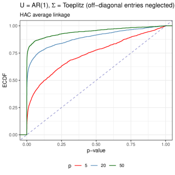
Figure 1: Empirical cumulative distribution functions (ECDF) of $p$-values defined in [16] testing for the difference in cluster means after performing a hierarchical clustering algorithm (HAC) with average linkage. The ECDF were computed from $M=2000$ realizations of a matrix normal model with $\boldsymbol{\mu}=\mathbf{0}_{n\times p}$ and non-diagonal covariance matrices encoding the dependence between observations and features. For each realization, the test compared the means of two randomly selected clusters after setting the HAC to choose three clusters. $p$-values were computed by assuming (1), setting $n=100$ and $p\in\{5,20,50\}$.

The practical motivation of the present work is to perform inference after clustering protein conformations. Protein structures are non-static and their conformational variability is essential to understand the relationship between sequence, structural properties and function [21]. Due to the high complexity of the conformational space, clustering techniques have emerged as powerful tools to characterize the structural variability of proteins, by extracting families of representative states [10, 3, 36, 32]. Usually, Euclidean distances between pairs of amino acids are considered as $p$-dimensional descriptors of protein conformations [10, 22, 7]. These distances are highly correlated and hardly match the model (1). Moreover, protein data is often simulated with Molecular Dynamics approaches that simulate the time-evolution of the protein according to physical models [2]. In that case, independence between observations cannot be assumed.

Accordingly, our aim is to go one step further and extend the framework introduced in [16] to a more general setting where arbitrary dependence structures between observations and features are admitted. We present an adaptation of [16] where the model (1) is extended to

$$\mathbf{X}\sim\mathcal{MN}_{n\times p}(\boldsymbol{\mu},\mathbf{U},\mathbf{\Sigma}),$$ (2)

where $\boldsymbol{\mu}\in\mathcal{M}_{n\times p}(\mathbb{R})$, $\mathbf{U}\in\mathcal{M}_{n\times n}(\mathbb{R})$ and $\mathbf{\Sigma}\in\mathcal{M}_{p\times p}(\mathbb{R})$. Our techniques follow the same reasoning steps as the ones in [16] and show that a $p$-value for testing differences between estimated cluster means can be defined under (2). The paper is organized as follows:

• Section 2 presents the definition of a $p$-value for post-clustering inference under the general model (2), and show that its efficient computation is straightforward if it is achievable under (1).

• In Section 3, we explore the scenarios that allow the asymptotic over-estimation of either $\mathbf{U}$ or $\mathbf{\Sigma}$ while respecting the asymptotic control of the selective type I error. We provide an estimator that can be used in several common practical scenarios.

• In Section 4, we revisit the framework presented in Section 2 when, for technical reasons, additional information is imposed to the conditioning event that defines the $p$-value. In particular, this enables selective inference after $k$-means clustering, following [9].

• Section 5 illustrates all the results through numerical experiments on synthetic data. Finally, Section 6 shows how this theory can be applied to perform inference after clustering protein structures.

Selective inference for clustering under general dependency

In [16], the authors consider the problem of selective inference after hierarchical clustering in the case of independent observations and features. Here, we aim to extend the method to admit general dependence structures. We consider $n$ observations of $p$ features drawn from the matrix normal distribution (2), where $\mathbf{U}$ and $\mathbf{\Sigma}$ are required to be positive definite. Each row of $\mathbf{X}$ is a vector of features in $\mathbb{R}^{p}$. The dependence between such features is given by $\mathbf{\Sigma}$, and $\mathbf{U}$ encodes the dependency between observations. If observations are independent with unit variance, we have $\mathbf{U}=\mathbf{I}_{n}$, and if features are independent with equal variance we can write $\mathbf{\Sigma}=\sigma^{2}\mathbf{I}_{p}$ for a given $\sigma>0$. These two assumptions define the model in [16]. Here, we show that this model can be generalized to arbitrary $\mathbf{U}$, $\mathbf{\Sigma}$, defining a $p$-value that controls the selective type I error rate for clustering.

Let us first recall the setting introduced in [16]. We will denote by $X_{i}$ (resp. $\mu_{i}$) the $i$-th row of $\mathbf{X}$ (resp. $\boldsymbol{\mu}$) and, for a group of observations $\mathcal{G}\subseteq\{1,\ldots,n\}$, $X_{\mathcal{G}}$ will denote the submatrix of $\mathbf{X}$ with rows $X_{i}$ for $i\in\mathcal{G}$. We also consider the mean of $\mathcal{G}$ in $\mathbf{X}$, denoted by

$$\bar{\mu}_{\mathcal{G}}=\frac{1}{\left\lvert\mathcal{G}\right\rvert}\sum_{i\in\mathcal{G}}\mu_{i},$$ (3)

and its empirical counterpart

$$\bar{X}_{\mathcal{G}}=\frac{1}{\left\lvert\mathcal{G}\right\rvert}\sum_{i\in\mathcal{G}}X_{i}.$$ (4)

From now on, we use the notation $\mathbf{M}=\left(M_{ij}\right)_{ij}$ to denote real matrices. Let $\mathcal{C}$ be a clustering algorithm, $\mathbf{x}$ a realization of the random variable $\mathbf{X}$ and $\hat{C}_{1},\hat{C}_{2}$ an arbitrary pair of clusters in $\mathcal{C}(\mathbf{x})$. The goal of post-clustering inference is to assess the null hypothesis

$$H_{0}^{\{\hat{C}_{1},\hat{C}_{2}\}}:\bar{\mu}_{\hat{C}_{1}}=\bar{\mu}_{\hat{C}_{2}}$$ (5)

by controlling the selective type I error for clustering at level $\alpha$, i.e. by ensuring that

$$\mathbb{P}_{H_{0}^{\{\hat{C}_{1},\hat{C}_{2}\}}}\left(\textrm{reject }H_{0}^{\{\hat{C}_{1},\hat{C}_{2}\}}\textrm{ based on }\mathbf{X}\textrm{ at level }\alpha\,\,\biggr{\rvert}\,\,\hat{C}_{1},\hat{C}_{2}\in\mathcal{C}(\mathbf{X})\right)\leq\alpha\quad\forall\,\alpha\in[0,1].$$ (6)

The ideal scenario to define a $p$-value for (5) satisfying (6) would be to only condition on the event $\{\hat{C}_{1},\hat{C}_{2}\in\mathcal{C}(\mathbf{X})\}$, which is the broader conditioning set that allows selective type I error control. However, making the $p$-value analytically tractable often needs the refinement of the conditioning set by adding more technical events (see also Section 4). In [16], the authors consider a test statistic of the form $\left\lVert\bar{X}_{\hat{C}_{1}}-\bar{X}_{\hat{C}_{2}}\right\rVert_{2}$ and introduce the quantity

$$p(\mathbf{x};\{\hat{C}_{1},\hat{C}_{2}\})=\mathbb{P}_{H_{0}^{\{\hat{C}_{1},\hat{C}_{2}\}}}\left(\left\lVert\bar{X}_{\hat{C}_{1}}-\bar{X}_{\hat{C}_{2}}\right\rVert_{2}\geq\left\lVert\bar{x}_{\hat{C}_{1}}-\bar{x}_{\hat{C}_{2}}\right\rVert_{2}\,\,\biggr{\lvert}\,\,\hat{C}_{1},\hat{C}_{2}\in\mathcal{C}(\mathbf{X}),\right.$$

$$\left.\boldsymbol{\pi}_{\nu(\hat{C}_{1},\hat{C}_{2})}^{\perp}\mathbf{X}=\boldsymbol{\pi}_{\nu(\hat{C}_{1},\hat{C}_{2})}^{\perp}\mathbf{x}\,,\,\mathrm{dir}\left(\bar{X}_{\hat{C}_{1}}-\bar{X}_{\hat{C}_{2}}\right)=\mathrm{dir}\left(\bar{x}_{\hat{C}_{1}}-\bar{x}_{\hat{C}_{2}}\right)\right),$$ (7)

where $\pi_{\nu}^{\perp}=\mathbf{I}_{n}-\nu\nu^{T}/\left\lVert\nu\right\rVert_{2}^{2}$, $\mathrm{dir}(u)=u/\left\lVert u\right\rVert_{2}\mathds{1}\{u\neq 0\}$ and the components of $\nu(\hat{C}_{1},\hat{C}_{2})$ are defined as

$$\nu(\hat{C}_{1},\hat{C}_{2})_{i}=\mathds{1}\{i\in\hat{C}_{1}\}/|\hat{C}_{1}|-\mathds{1}\{i\in\hat{C}_{2}\}/|\hat{C}_{2}|.$$ (8)

Theorem 1 in [16] proves that (2) is a $p$-value for (5). Moreover, if $\mathcal{C}$ is a hierarchical clustering algorithm, the $p$-value (2) can be explicitly characterized and efficiently computed for several types of linkages. Otherwise, it can be approximated with a Monte Carlo procedure.

Here, we aim at extending (2) for the general model (2). The main idea is to replace the norm $\left\lVert\cdot\right\rVert_{2}$ in the test statistic by the more general norm

$$\left\lVert x\right\rVert_{\mathbf{V}_{\hat{C}_{1},\hat{C}_{2}}}=\sqrt{x^{T}\mathbf{V}_{\hat{C}_{1},\hat{C}_{2}}^{-1}x},\quad\forall\,x\in\mathbb{R}^{p},$$ (9)

where $\mathbf{V}_{\hat{C}_{1},\hat{C}_{2}}\in\mathcal{M}_{p\times p}(\mathbb{R})$ integrates the information about the scale matrices in (2). Let us first introduce some notation. For a pair of non-overlapping groups of observations $\mathcal{G}_{1},\mathcal{G}_{2}\subseteq\{1,\ldots,n\}$, we define the $p(\left\lvert\mathcal{G}_{1}\right\rvert+\left\lvert\mathcal{G}_{2}\right\rvert)$ column vector

$$X_{\mathcal{G}_{1},\mathcal{G}_{2}}=(\mathrm{vec}(X_{\mathcal{G}_{1}}^{T}),\mathrm{vec}(X_{\mathcal{G}_{2}}^{T})),$$ (10)

which concatenates the column vectors of observations in $\mathcal{G}_{1}$ with the ones in $\mathcal{G}_{2}$. Similarly, we denote as $\mathbf{U}_{\mathcal{G}_{1},\mathcal{G}_{2}}$ the principal submatrix of $\mathbf{U}$ containing the rows and columns in $\mathcal{G}_{1}\cup\mathcal{G}_{2}$. Finally, we consider $\mathbf{D}_{\mathcal{G}_{1},\mathcal{G}_{2}}\in\mathcal{M}_{p\times p(\left\lvert\mathcal{G}_{1}\right\rvert+\left\lvert\mathcal{G}_{2}\right\rvert)}$ the linear operator verifying $\mathbf{D}_{\mathcal{G}_{1},\mathcal{G}_{2}}X_{\mathcal{G}_{1},\mathcal{G}_{2}}=\bar{X}_{\mathcal{G}_{1}}-\bar{X}_{\mathcal{G}_{2}}$, that we can write explicitly as the block matrix

$$\mathbf{D}_{\mathcal{G}_{1},\mathcal{G}_{2}}=\begin{pmatrix}\frac{1}{\left\lvert\mathcal{G}_{1}\right\rvert}\mathbf{I}_{p}&\overset{\left\lvert\mathcal{G}_{1}\right\rvert}{\cdots}&\frac{1}{\left\lvert\mathcal{G}_{1}\right\rvert}\mathbf{I}_{p}&-\frac{1}{\left\lvert\mathcal{G}_{2}\right\rvert}\mathbf{I}_{p}&\overset{\left\lvert\mathcal{G}_{2}\right\rvert}{\cdots}&-\frac{1}{\left\lvert\mathcal{G}_{2}\right\rvert}\mathbf{I}_{p}\end{pmatrix}.$$ (11)

We can now define the matrix $\mathbf{V}_{\mathcal{G}_{1},\mathcal{G}_{2}}$ in (9) as

$$\mathbf{V}_{\mathcal{G}_{1},\mathcal{G}_{2}}=\mathbf{D}_{\mathcal{G}_{1},\mathcal{G}_{2}}(\mathbf{U}_{\mathcal{G}_{1},\mathcal{G}_{2}}\otimes\mathbf{\Sigma})\mathbf{D}_{\mathcal{G}_{1},\mathcal{G}_{2}}^{T},$$ (12)

where $\otimes$ denotes the Kronecker product of matrices. Note that (9) is a well-defined norm if and only if $\mathbf{V}_{\mathcal{G}_{1},\mathcal{G}_{2}}$ is a positive definite matrix, which here is guaranteed as $\mathbf{D}_{\mathcal{G}_{1},\mathcal{G}_{2}}$ has full rank and $\mathbf{U}$ and $\mathbf{\Sigma}$ are positive definite [19]. The following result extends Theorem 1 in [16] by proving that the quantity

$$p_{\mathbf{V}_{\hat{C}_{1},\hat{C}_{2}}}(\mathbf{x};\{\hat{C}_{1},\hat{C}_{2}\})=\mathbb{P}_{H_{0}^{\{\hat{C}_{1},\hat{C}_{2}\}}}\left(\left\lVert\bar{X}_{\hat{C}_{1}}-\bar{X}_{\hat{C}_{2}}\right\rVert_{\mathbf{V}_{\hat{C}_{1},\hat{C}_{2}}}\geq\left\lVert\bar{x}_{\hat{C}_{1}}-\bar{x}_{\hat{C}_{2}}\right\rVert_{\mathbf{V}_{\hat{C}_{1},\hat{C}_{2}}}\,\,\biggr{\rvert}\,\,\hat{C}_{1},\hat{C}_{2}\in\mathcal{C}(\mathbf{X}),\right.$$

$$\left.\boldsymbol{\pi}_{\nu(\hat{C}_{1},\hat{C}_{2})}^{\perp}\mathbf{X}=\boldsymbol{\pi}_{\nu(\hat{C}_{1},\hat{C}_{2})}^{\perp}\mathbf{x}\,,\,\mathrm{dir}_{\mathbf{V}_{\hat{C}_{1},\hat{C}_{2}}}\left(\bar{X}_{\hat{C}_{1}}-\bar{X}_{\hat{C}_{2}}\right)=\mathrm{dir}_{\mathbf{V}_{\hat{C}_{1},\hat{C}_{2}}}\left(\bar{x}_{\hat{C}_{1}}-\bar{x}_{\hat{C}_{2}}\right)\right),$$ (13)

where $\mathrm{dir}_{\mathbf{V}_{\hat{C}_{1},\hat{C}_{2}}}(u)=u/\left\lVert u\right\rVert_{\mathbf{V}_{\hat{C}_{1},\hat{C}_{2}}}\mathds{1}\{u\neq 0\}$, is a computationally tractable $p$-value for (5) that controls the selective type I error rate for arbitrary dependence structures $\mathbf{U},\mathbf{\Sigma}$.

Theorem 2.1.

Let $\mathbf{x}$ be a realization of $\mathbf{X}$ and $\mathcal{G}_{1},\mathcal{G}_{2}\in\mathcal{P}(\{1,\ldots,n\})$ with $\mathcal{G}_{1}\cap\mathcal{G}_{2}=\emptyset$. Then, $p_{\mathbf{V}_{\mathcal{G}_{1},\mathcal{G}_{2}}}(\mathbf{x};\{\mathcal{G}_{1},\mathcal{G}_{2}\})$ is a $p$-value for the test $H_{0}^{\{\mathcal{G}_{1},\mathcal{G}_{2}\}}$: $\bar{\mu}_{\mathcal{G}_{1}}=\bar{\mu}_{\mathcal{G}_{2}}$ that controls the selective type I error for clustering (6) at level $\alpha$. Furthermore, it satisfies

$$p_{\mathbf{V}_{\mathcal{G}_{1},\mathcal{G}_{2}}}(\mathbf{x};\{\mathcal{G}_{1},\mathcal{G}_{2}\})=1-\mathbb{F}_{p}\left(\left\lVert\bar{x}_{\mathcal{G}_{1}}-\bar{x}_{\mathcal{G}_{2}}\right\rVert_{\mathbf{V}_{\mathcal{G}_{1},\mathcal{G}_{2}}},\,\mathcal{S}_{\mathbf{V}_{\mathcal{G}_{1},\mathcal{G}_{2}}}(\mathbf{x};\{\mathcal{G}_{1},\mathcal{G}_{2}\})\right),$$ (14)

where $\mathbb{F}_{p}(t,\mathcal{S})$ is the cumulative distribution function of a $\chi_{p}$ random variable truncated to the set $\mathcal{S}$ and

$$\mathcal{S}_{\mathbf{V}_{\mathcal{G}_{1},\mathcal{G}_{2}}}(\mathbf{x};\{\mathcal{G}_{1},\mathcal{G}_{2}\})=\left\{\phi\geq 0\,:\,\mathcal{G}_{1},\mathcal{G}_{2}\in\mathcal{C}\left(\boldsymbol{\pi}_{\nu(\mathcal{G}_{1},\mathcal{G}_{2})}^{\perp}\mathbf{x}+\left(\frac{\phi}{\frac{1}{\left\lvert\mathcal{G}_{1}\right\rvert}+\frac{1}{\left\lvert\mathcal{G}_{2}\right\rvert}}\right)\nu(\mathcal{G}_{1},\mathcal{G}_{2})\mathrm{dir}_{\mathbf{V}_{\mathcal{G}_{1},\mathcal{G}_{2}}}(\bar{x}_{\mathcal{G}_{1}}-\bar{x}_{\mathcal{G}_{2}})\right)\right\}.$$ (15)

Theorem 2.1 is proved in Appendix A. One can easily verify that replacing $\mathbf{U}=\mathbf{I}_{n}$ and $\mathbf{\Sigma}=\sigma^{2}\mathbf{I}_{p}$ in Theorem 2.1 yields exactly Theorem 1 in [16]. The only difference is that, here, the information about the variance has been extracted from the statistic null distribution, which now remains the same independently of $\mathbf{U},\mathbf{\Sigma}$, and moved it into the test statistic itself by making it dependent on the scale matrices. Note that this formulation replaces the Euclidean distance considered in [16] by the Mahalanobis distance [26]. Recall that, if $x,y\in\mathbb{R}^{p}$ and $P$ is a probability distribution supported on $\mathbb{R}^{p}$ with covariance matrix $C$, the Mahalanobis distance between $x$ and $y$ with respect to $P$ is given by $\left\lVert x-y\right\rVert_{C}$, where $\left\lVert\cdot\right\rVert_{C}$ is defined as (9). Consequently, the formulation in Theorem 2.1 corresponds to consider as statistic the Mahalanobis distance between the empirical means $\bar{X}_{\hat{C}_{1}}$ and $\bar{X}_{\hat{C}_{2}}$ with respect to the null distribution of their difference $\bar{X}_{\hat{C}_{1}}-\bar{X}_{\hat{C}_{2}}$, which is a centered multivariate normal of covariance matrix $\mathbf{V}_{\hat{C}_{1},\hat{C}_{2}}$ (see proof of Theorem 2.1). This distance generalizes to multiple dimensions the idea of quantifying how many standard deviations away a point is from the mean of its distribution, and therefore integrates the dependence structure between columns and rows in $\mathbf{X}$.

Following (14), computing the $p$-value (2) only depends on the characterization of the one-dimensional set

$$\hat{\mathcal{S}}_{\mathbf{V}_{\hat{C}_{1},\hat{C}_{2}}}=\mathcal{S}_{\mathbf{V}_{\hat{C}_{1},\hat{C}_{2}}}(\mathbf{x};\{\hat{C}_{1},\hat{C}_{2}\})=\left\{\phi\geq 0\,:\,\hat{C}_{1},\hat{C}_{2}\in\mathcal{C}\left(\mathbf{x}^{\prime}_{\mathbf{V}_{\hat{C}_{1},\hat{C}_{2}}}(\phi)\right)\right\},$$ (16)

where the set $\mathcal{S}_{\mathbf{V}_{\hat{C}_{1},\hat{C}_{2}}}(\mathbf{x},\cdot)$ is defined in (15) and

$$\mathbf{x}^{\prime}_{\mathbf{V}_{\hat{C}_{1},\hat{C}_{2}}}(\phi)=\boldsymbol{\pi}_{\nu(\hat{C}_{1},\hat{C}_{2})}^{\perp}\mathbf{x}+\left(\frac{\phi}{\frac{1}{\left\lvert\hat{C}_{1}\right\rvert}+\frac{1}{\left\lvert\hat{C}_{2}\right\rvert}}\right)\nu(\hat{C}_{1},\hat{C}_{2})\mathrm{dir}_{\mathbf{V}_{\hat{C}_{1},\hat{C}_{2}}}(\bar{x}_{\hat{C}_{1}}-\bar{x}_{\hat{C}_{2}}).$$ (17)

The data set (17) is analogous to $\mathbf{x}^{\prime}(\phi)$ in [16, Equation (13)] for the norm (9), and its interpretation is equivalent. Indeed, we can rewrite both $\mathbf{x}^{\prime}(\phi)$ and (17) as

$$\mathbf{x}^{\prime}(\phi)=\mathbf{x}+\frac{\nu(\hat{C}_{1},\hat{C}_{2})}{\left\lVert\nu(\hat{C}_{1},\hat{C}_{2})\right\rVert_{2}^{2}}\left(\phi-\left\lVert\bar{x}_{\hat{C}_{1}}-\bar{x}_{\hat{C}_{2}}\right\rVert_{2}\right)\mathrm{dir}(\bar{x}_{\hat{C}_{1}}-\bar{x}_{\hat{C}_{2}}),$$ (18)

$$\mathbf{x}^{\prime}_{\mathbf{V}_{\hat{C}_{1},\hat{C}_{2}}}(\phi)=\mathbf{x}+\frac{\nu(\hat{C}_{1},\hat{C}_{2})}{\left\lVert\nu(\hat{C}_{1},\hat{C}_{2})\right\rVert_{2}^{2}}\left(\phi-\left\lVert\bar{x}_{\hat{C}_{1}}-\bar{x}_{\hat{C}_{2}}\right\rVert_{\mathbf{V}_{\hat{C}_{1},\hat{C}_{2}}}\right)\mathrm{dir}_{\mathbf{V}_{\hat{C}_{1},\hat{C}_{2}}}(\bar{x}_{\hat{C}_{1}}-\bar{x}_{\hat{C}_{2}}).$$ (19)

Consequently, we can interpret (17) as a perturbed version $\mathbf{x}^{\prime}(\phi)$ of $\mathbf{x}$, but where the perturbation is based on the norm $\left\lVert\cdot\right\rVert_{\mathbf{V}_{\hat{C}_{1},\hat{C}_{2}}}$ defined in (9) instead of $\left\lVert\cdot\right\rVert_{2}$. Thus, the set (16) is the set of non-negative $\phi$ for which applying the clustering algorithm $\mathcal{C}$ to the perturbed data set $\mathbf{x}^{\prime}_{\mathbf{V}_{\hat{C}_{1},\hat{C}_{2}}}(\phi)$ yields $\hat{C}_{1}$ and $\hat{C}_{2}$. As shown in [16], the set

$$\hat{\mathcal{S}}=\{\phi\geq 0\,:\,\hat{C}_{1},\hat{C}_{2}\in\mathcal{C}(\mathbf{x}^{\prime}(\phi))\},$$ (20)

can be explicitly characterized for hierarchical clustering. Importantly, we do not need to re-adapt the work in [16] to the set (16), as its points are given by a scale transformation of the points in $\hat{\mathcal{S}}$:

Lemma 2.2.

Let $\mathbf{x}$ be a realization of $\mathbf{X}$ and $\hat{C}_{1},\hat{C}_{2}$ an arbitrary pair of clusters in $\mathcal{C}(\mathbf{x})$. Let $\hat{\mathcal{S}}$ denote the set (20) defined in [16, Equation (12)]. Then,

$$\hat{\mathcal{S}}_{\mathbf{V}_{\hat{C}_{1},\hat{C}_{2}}}=\frac{\left\lVert\bar{x}_{\hat{C}_{1}}-\bar{x}_{\hat{C}_{2}}\right\rVert_{\mathbf{V}_{\hat{C}_{1},\hat{C}_{2}}}}{\left\lVert\bar{x}_{\hat{C}_{1}}-\bar{x}_{\hat{C}_{2}}\right\rVert_{2}}\,\hat{\mathcal{S}},$$ (21)

where $\hat{\mathcal{S}}_{\mathbf{V}_{\hat{C}_{1},\hat{C}_{2}}}$ is defined in (16).

Consequently, the work in [16, Section 3] can be applied here to characterize the set (16) and, therefore, to compute the $p$-value defined in (2). An explicit characterization of (16) is possible when $\mathcal{C}$ is a hierarchical clustering algorithm with squared Euclidean distance, along with either single linkage or a linkage satisfying a linear Lance-Williams update [16, Equation 20], e.g. average, weighted, Ward, centroid or median linkage. The efficient computation of $\eqref{set_S_hat}$ can also be extended to $k$-means clustering, as shown in Section 4. Otherwise, the $p$-value (2) can be approximated with a Monte Carlo procedure, adapting the importance sampling approach presented in [16, Section 4.1]. Following the same notation, we sample

$$\omega_{1},\ldots,\omega_{N}\overset{i.i.d.}{\sim}\mathcal{N}\left(\left\lVert\bar{x}_{\hat{C}_{1}}-\bar{x}_{\hat{C}_{2}}\right\rVert_{\mathbf{V}_{\hat{C}_{1},\hat{C}_{2}}},1\right)$$

and approximate (2) as

$$p_{\mathbf{V}_{\hat{C}_{1},\hat{C}_{2}}}(\mathbf{x};\{\hat{C}_{1},\hat{C}_{2}\})\approx\frac{\sum_{i=1}^{N}\,\pi_{i}\,\mathds{1}\left\{\omega_{i}\geq\left\lVert\bar{x}_{\hat{C}_{1}}-\bar{x}_{\hat{C}_{2}}\right\rVert_{\mathbf{V}_{\hat{C}_{1},\hat{C}_{2}}},\hat{C}_{1},\hat{C}_{2}\in\mathcal{C}(\mathbf{x}^{\prime}(\omega_{i}))\right\}}{\sum_{i=1}^{N}\,\pi_{i}\,\mathds{1}\left\{\hat{C}_{1},\hat{C}_{2}\in\mathcal{C}(\mathbf{x}^{\prime}(\omega_{i}))\right\}},$$ (22)

for $\pi_{i}=f_{1}(\omega_{i})/f_{2}(\omega_{i})$, where $f_{1}$ is the density of a $\chi_{p}$ random variable, and $f_{2}$ is the density of a $\mathcal{N}(\left\lVert\bar{x}_{\hat{C}_{1}}-\bar{x}_{\hat{C}_{2}}\right\rVert_{\mathbf{V}_{\hat{C}_{1},\hat{C}_{2}}},1)$ random variable.

Unknown dependence structures

The selective inference framework introduced for model (2) in Section 2 assumes that both scale matrices $\mathbf{U}$ and $\mathbf{\Sigma}$ are known, which is a quite unrealistic scenario. Under the independence assumption made in [16], where $\mathbf{\Sigma}=\sigma^{2}\mathbf{I}_{p}$ and $\mathbf{U}=\mathbf{I}_{n}$, the authors showed in Theorem 4 that over-estimating $\sigma$ yields asymptotic control of the selective type I error, and provided such an estimator $\hat{\sigma}$ that can be used in practice. Under the general model (2), the scale matrices $\mathbf{U}$ and $\mathbf{\Sigma}$ are non-identifiable:

$$\mathbf{X}\sim\mathcal{MN}_{np}(\boldsymbol{\mu},\mathbf{U},\mathbf{\Sigma})\Leftrightarrow\mathbf{X}\sim\mathcal{N}_{np}(\boldsymbol{\mu},a\mathbf{U}\otimes a^{-1}\mathbf{\Sigma})\quad\textrm{for any }a>0,$$ (23)

so different parametrizations can yield the same distribution. This makes their simultaneous estimation an arduous task in practice. Non-unique Maximum Likelihood Estimates (MLE) exist for $\mathbf{U}$ and $\mathbf{\Sigma}$ [13], which depend on each other and can be computed through an iterative algorithm. However, even in the unlikely scenario where we had access to enough realizations of $\mathbf{X}$, the interdependence of the computed MLEs would still prevent us from assessing the control of selective type I error after estimation. In this Section, we investigate the situation where only one of the scale matrices is known, and assess theoretical conditions that allow asymptotic control of the selective type I error when estimating the other one. We also provide an estimator that satisfies these conditions for some common dependence models.

Let us recall that, for the model (2), we have

$$\mathbf{X}\sim\mathcal{M}\mathcal{N}_{n\times p}(\boldsymbol{\mu},\mathbf{U},\mathbf{\Sigma})\Leftrightarrow\mathbf{X}^{T}\sim\mathcal{M}\mathcal{N}_{p\times n}(\boldsymbol{\mu}^{T},\mathbf{\Sigma},\mathbf{U}).$$ (24)

Therefore, the methods presented in this Section can be equally applied to estimate $\mathbf{U}$ or $\mathbf{\Sigma}$ when the other is known, by transposing $\mathbf{X}$ if needed. From now on, we assume that the dependence structure between observations $\mathbf{U}$ is known, and study under which conditions we can suitably estimate $\mathbf{\Sigma}$. In other words, if $\hat{\mathbf{\Sigma}}(\mathbf{x})$ is an estimate of $\mathbf{\Sigma}$ for a given realization $\mathbf{x}$ of $\mathbf{X}$, we study under which conditions the $p$-value

$$p_{\hat{\mathbf{V}}_{\mathcal{G}_{1},\mathcal{G}_{2}}}(\mathbf{x};\{\mathcal{G}_{1},\mathcal{G}_{2}\})=1-\mathbb{F}_{p}\left(\left\lVert\bar{x}_{\mathcal{G}_{1}}-\bar{x}_{\mathcal{G}_{2}}\right\rVert_{\hat{\mathbf{V}}_{\mathcal{G}_{1},\mathcal{G}_{2}}};\,\mathcal{S}_{\hat{\mathbf{V}}_{\mathcal{G}_{1},\mathcal{G}_{2}}}(\mathbf{x};\{\mathcal{G}_{1},\mathcal{G}_{2}\})\right),$$ (25)

where $\hat{\mathbf{V}}_{\mathcal{G}_{1},\mathcal{G}_{2}}=\mathbf{D}_{\mathcal{G}_{1},\mathcal{G}_{2}}(\mathbf{U}_{\mathcal{G}_{1},\mathcal{G}_{2}}\otimes\hat{\mathbf{\Sigma}}(\mathbf{x}))\mathbf{D}_{\mathcal{G}_{1},\mathcal{G}_{2}}^{T}$, asymptotically controls the selective type I error. Theorem 3.1 generalizes Theorem 4 in [16] for the estimation of $\mathbf{\Sigma}$ under model (2) by relying on the Loewner partial order, defined below. The proof is included in Appendix B.

Definition 3.1 (Definition 7.7.1 in [19]).

Let $A,B$ be two square matrices of equal size. The binary relation $A\succeq B$ if and only if $A,B$ are Hermitian and $A-B$ is positive semidefinite is called the Loewner partial order between square matrices.

Theorem 3.1.

For $n\in\mathbb{N}$, let $\mathbf{X}^{(n)}\sim\mathcal{M}\mathcal{N}_{n\times p}(\boldsymbol{\mu}^{(n)},\mathbf{U}^{(n)},\mathbf{\Sigma})$. Let $\mathbf{x}^{(n)}$ be a realization of $\mathbf{X}^{(n)}$ and $\hat{C}_{1}^{(n)},\hat{C}_{2}^{(n)}$ a pair of clusters estimated from $\mathbf{x}^{(n)}$. If $\hat{\mathbf{\Sigma}}\left(\mathbf{X}^{(n)}\right)$ is a positive definite estimator of $\mathbf{\Sigma}$ such that

$$\underset{n\rightarrow\infty}{\lim}\mathbb{P}_{H_{0}^{\{\hat{C}_{1}^{(n)},\hat{C}_{2}^{(n)}\}}}\left(\hat{\mathbf{\Sigma}}\left(\mathbf{X}^{(n)}\right)\succeq\mathbf{\Sigma}\,\bigg{\rvert}\,\hat{C}_{1}^{(n)},\hat{C}_{2}^{(n)}\in\mathcal{C}\left(\mathbf{X}^{(n)}\right)\right)=1,$$ (26)

then, for any $\alpha\in[0,1]$, we have

$$\underset{n\rightarrow\infty}{\limsup}\,\mathbb{P}_{H_{0}^{\{\hat{C}_{1}^{(n)},\hat{C}_{2}^{(n)}\}}}\left(p_{\hat{\mathbf{V}}_{\hat{C}_{1}^{(n)},\hat{C}_{2}^{(n)}}}\left(\mathbf{X}^{(n)};\left\{\hat{C}_{1}^{(n)},\hat{C}_{2}^{(n)}\right\}\right)\leq\alpha\,\bigg{\rvert}\,\hat{C}_{1}^{(n)},\hat{C}_{2}^{(n)}\in\mathcal{C}\left(\mathbf{X}^{(n)}\right)\right)\leq\alpha,$$ (27)

where $p_{\hat{\mathbf{V}}_{\hat{C}_{1}^{(n)},\hat{C}_{2}^{(n)}}}$ is defined in (25).

Note that the Loewner partial order is a natural extension to Hermitian matrices of the usual order in $\mathbb{R}$. If we replace $\mathbf{\Sigma}$ by $\sigma^{2}\mathbf{I}_{p}$ in Theorem 3.1, the condition $\hat{\mathbf{\Sigma}}\succeq\mathbf{\Sigma}$ becomes $\hat{\sigma}\geq\sigma$, as in [16, Theorem 4]. We aim now at providing an estimator of $\mathbf{\Sigma}$ satisfying the conditions in Theorem 3.1. The asymptotic properties of such an estimator strongly depend on the asymptotic dependence structure between observations, given by the sequence of matrices $\{\mathbf{U}^{(n)}\}_{n\in\mathbb{N}}$ of Theorem 3.1. First, let us consider

$$\hat{\mathbf{\Sigma}}=\hat{\mathbf{\Sigma}}\left(\mathbf{X}\right)=\frac{1}{n-1}\left(\mathbf{X}-\bar{\mathbf{X}}\right)^{T}\mathbf{U}^{-1}\left(\mathbf{X}-\bar{\mathbf{X}}\right),$$ (28)

where $\bar{\mathbf{X}}$ is a $n\times p$ matrix having as rows the mean across rows of $\mathbf{X}$, i.e.

$$\bar{\mathbf{X}}=\mathbf{1}_{n}\otimes\frac{1}{n}\sum_{k=1}^{n}X_{k},$$ (29)

where $\mathbf{1}_{n}$ is a column $n$-vector of ones. We can also write (28) element-wise:

$$\hat{\Sigma}_{ij}=\frac{1}{n-1}\sum_{l,s=1}^{n}\left(X_{li}-\bar{X}_{i}\right)\left(U^{-1}\right)_{ls}\left(X_{sj}-\bar{X}_{j}\right),\quad\forall\,i,j\in\{1,\ldots,p\},$$ (30)

where $\bar{X}_{i}=\frac{1}{n}\sum_{k=1}^{n}X_{ki}$. Note that the estimator $\hat{\mathbf{\Sigma}}$ is a positive definite matrix if the matrix $\mathbf{X}-\bar{\mathbf{X}}$ has full rank. In that case, (28) satisfies the conditions of Theorem 3.1 if we make some assumptions about how the matrices $\boldsymbol{\mu}^{(n)}$ and $\mathbf{U}^{(n)}$ in Theorem 3.1 grow up as $n$ increases. We first adopt the assumptions about $\{\boldsymbol{\mu}^{(n)}\}_{n\in\mathbb{N}}$ made in [16] to prove the counterpart of Theorem 3.1 for the independence scenario.

Assumption 3.1 (Assumptions 1 and 2 in [16]).

For all $n\in\mathbb{N}$, there are exactly $K^{*}$ distinct mean vectors among the first $n$ observations, i.e.

$$\left\{\mu_{i}^{(n)}\right\}_{i=1,\ldots,n}=\{\theta_{1},\ldots,\theta_{K^{*}}\}.$$ (31)

Moreover, the proportion of the first $n$ observations that have mean vector $\theta_{k}$ converges to $\pi_{k}>0$, i.e.

$$\underset{n\rightarrow\infty}{\lim}\frac{1}{n}\sum_{i=1}^{n}\mathds{1}\{\mu_{i}^{(n)}=\theta_{k}\}=\pi_{k},$$ (32)

for all $k\in\{1,\ldots,K^{*}\}$, where $\sum_{k=1}^{K^{*}}\pi_{k}=1$.

If observations are independent and we set $\mathbf{U}^{(n)}=\mathbf{I}_{n}$, Assumption 3.1 is the only requirement for (28) to asymptotically over-estimate $\mathbf{\Sigma}$ in the sense of Theorem 3.1. However, for general $\mathbf{U}^{(n)}$, the quantities

$$\frac{1}{n}\sum_{l,s=1}^{n}\left(U^{(n)}\right)^{-1}_{ls}\,\mathds{1}\{\mu_{l}^{(n)}=\theta_{k}\}\,\mathds{1}\{\mu_{s}^{(n)}=\theta_{k^{\prime}}\}$$ (33)

are also required to converge as $n$ tends to infinity. Furthermore, we need to know its limit explicitly to assess whether $\hat{\mathbf{\Sigma}}\succeq\mathbf{\Sigma}$ asymptotically. This requires relatively strong conditions on the sequence $\{\mathbf{U}^{(n)}\}_{n\in\mathbb{N}}$, which can be difficult to verify for a given model of dependence, as well as an additional mild condition on the sequence $\{\boldsymbol{\mu}^{(n)}\}_{n\in\mathbb{N}}$, needed for non-diagonal $\mathbf{U}^{(n)}$. Let’s begin by stating the latter.

Assumption 3.2.

If $\mathbf{U}^{(n)}$ is non-diagonal for all $n\in\mathbb{N}$, for any $k,k^{\prime}\in\{1,\ldots,K^{*}\}$, the proportion of the first $n$ observations at distance $r\geq 1$ in $\mathbf{X}^{(n)}$ having means $\theta_{k}$ and $\theta_{k^{\prime}}$ converges, and its limit converges to $\pi_{k}\pi_{k^{\prime}}$ when the lag $r$ tends to infinity. More precisely,

$$\underset{n\rightarrow\infty}{\lim}\frac{1}{n}\sum_{i=1}^{n-r}\mathds{1}\{\mu_{i}=\theta_{k}\}\,\mathds{1}\{\mu_{i+r}=\theta_{k^{\prime}}\}=\pi_{kk^{\prime}}^{r}\underset{r\rightarrow\infty}{\longrightarrow}\pi_{k}\,\pi_{k^{\prime}}.$$ (34)

Note that we are requiring the proportion of pairs of observations having a given a pair of means to approach the product of individual proportions (32) when both observations are far away in $\mathbf{X}^{(n)}$. Stronger conditions need to be imposed to the sequence $\{\mathbf{U}^{(n)}\}_{n\in\mathbb{N}}$ in order for (33) to converge with tractable limit.

Assumption 3.3.

Let $\{\mathbf{U}^{(n)}\}_{n\in\mathbb{N}}$ be a sequence of real positive definite matrices, and let $\left(U^{(n)}\right)^{-1}_{ij}$ denote the $i,j$ entry of $\left(\mathbf{U}^{(n)}\right)^{-1}$ for any $n\in\mathbb{N}$. Then, every superdiagonal of $\left(\mathbf{U}^{(n)}\right)^{-1}$ defines asymptotically a convergent sequence, whose limits sum up to a real value. More precisely, for any $i\in\mathbb{N}$ and any $r\geq 0$,

$$\underset{n\rightarrow\infty}{\lim}\,\left(U^{(n)}\right)^{-1}_{i\,i+r}=\Lambda_{i\,i+r},\,\quad\mathrm{where}\quad\underset{i\rightarrow\infty}{\lim}\Lambda_{i\,i+r}=\lambda_{r}\quad\mathrm{and}\quad\sum_{r=0}^{\infty}\lambda_{r}=\lambda\in\mathbb{R}.$$ (35)

Moreover, for each $r\geq 0$, the sequence $\{\left(U^{(n)}\right)^{-1}_{i\,i+r}\}_{n\in\mathbb{N}}$ satisfies any of the following conditions:

• It is dominated by a summable sequence i.e. $\left\lvert\left(U^{(n)}\right)^{-1}_{i\,i+r}-\Lambda_{i\,i+r}\right\rvert\leq\alpha_{i}\,\,\forall\,n\in\mathbb{N}$, with $\{\alpha_{i}\}_{i=1}^{\infty}\in\ell_{1}$,

• For each $i\in\mathbb{N}$, it is non-decreasing or non-increasing.

If Assumptions 3.1, 3.2 and 3.3 hold for a given pair of sequences $\{\boldsymbol{\mu}^{(n)}\}_{n\in\mathbb{N}}$, $\{\mathbf{U}^{(n)}\}_{n\in\mathbb{N}}$, the following result ensures that $\hat{\mathbf{\Sigma}}$ asymptotically over-estimates (in the sense of the Loewner partial order) the dependence structure $\mathbf{\Sigma}$ between features.

Proposition 3.2.

Let $\mathbf{X}^{(n)}\sim\mathcal{M}\mathcal{N}_{n\times p}(\boldsymbol{\mu}^{(n)},\mathbf{U}^{(n)},\mathbf{\Sigma})$, where $\boldsymbol{\mu}^{(n)}$ and $\mathbf{U}^{(n)}$ satisfy Assumptions 3.1, 3.2 and 3.3 for some $K^{*}>1$. Let $\hat{\mathbf{\Sigma}}$ be the estimator defined in (28). Then,

$$\underset{n\rightarrow\infty}{\lim}\,\mathbb{P}\left(\hat{\mathbf{\Sigma}}\left(\mathbf{X}^{(n)}\right)\succeq\mathbf{\Sigma}\right)=1.$$ (36)

Our proof of Proposition 3.2 relies of the following Lemma, which makes use of Assumptions 3.1, 3.2 and 3.3 explicitly. Both results are proved in Appendix B.

Lemma 3.3.

Let $\mathbf{X}^{(n)}\sim\mathcal{M}\mathcal{N}_{n\times p}(\boldsymbol{\mu}^{(n)},\mathbf{U}^{(n)},\mathbf{\Sigma})$, where $\boldsymbol{\mu}^{(n)}$ and $\mathbf{U}^{(n)}$ satisfy Assumptions 3.1, 3.2 and 3.3 for some $K^{*}>1$. Then,

$$\underset{n\rightarrow\infty}{\lim}\,\frac{1}{n}\sum_{l,s=1}^{n}\left(U^{(n)}\right)^{-1}_{ls}\,\mathds{1}\{\mu_{l}^{(n)}=\theta_{k}\}\,\mathds{1}\{\mu_{s}^{(n)}=\theta_{k^{\prime}}\}=2(\lambda-\lambda_{0})\pi_{k}\pi_{k^{\prime}}+\lambda_{0}\pi_{k}\delta_{kk^{\prime}},$$ (37)

for any $k,k^{\prime}\in\{1,\ldots,K^{\prime}\}$, and where $\pi_{k},\pi_{k^{\prime}}$ and $\lambda_{0},\lambda$ are defined in Assumptions 3.1 and 3.3 respectively.

Finally, it suffices to estimate $\mathbf{\Sigma}$ using an independent and identically distributed copy of $\mathbf{X}^{(n)}$ to have (26) provided (36). Combined this observation with Proposition 3.2, we obtain our final result:

Proposition 3.4.

Let $\mathbf{X}^{(n)}\sim\mathcal{M}\mathcal{N}_{n\times p}(\boldsymbol{\mu}^{(n)},\mathbf{U}^{(n)},\mathbf{\Sigma})$, where $\boldsymbol{\mu}^{(n)}$ and $\mathbf{U}^{(n)}$ satisfy Assumptions 3.1, 3.2 and 3.3 for some $K^{*}>1$. Let $\mathbf{x}^{(n)}$ be a realization of $\mathbf{X}^{(n)}$ and $\hat{C}_{1}^{(n)}$, $\hat{C}_{2}^{(n)}$ a pair of clusters estimated from $\mathbf{x}^{(n)}$. Let $\mathbf{Y}^{(n)}$ an independent and identically distributed copy of $\mathbf{X}^{(n)}$. Then, the estimator $\hat{\mathbf{\Sigma}}\left(\mathbf{Y}^{(n)}\right)$ defined in (28) satisfies the conditions of Theorem 3.1, i.e.

$$\underset{n\rightarrow\infty}{\lim}\mathbb{P}_{H_{0}^{\{\hat{C}_{1}^{(n)},\hat{C}_{2}^{(n)}\}}}\left(\hat{\mathbf{\Sigma}}\left(\mathbf{Y}^{(n)}\right)\succeq\mathbf{\Sigma}\,\bigg{\rvert}\,\hat{C}_{1}^{(n)},\hat{C}_{2}^{(n)}\in\mathcal{C}\left(\mathbf{X}^{(n)}\right)\right)=1.$$ (38)

Assessing whether a model of dependence satisfies the hypotheses of Proposition 3.4 (more precisely, Assumption 3.3) is not trivial as it requires full knowledge of how the inverse matrices $\left(\mathbf{U}^{(n)}\right)^{-1}$ grow up when dimension increases. However, we are able to show that Assumption 3.3 is satisfied for some simple dependence models and, consequently, that selective type I error can be controlled when $\mathbf{\Sigma}$ is estimated in such cases. The following remarks are proved in Appendix B.

Remark 3.1 (Diagonal).

Let $\mathbf{U}^{(n)}=\mathrm{diag}(\lambda_{1},\ldots,\lambda_{n})$. If the sequence $\{\lambda_{n}\}_{n\in\mathbb{N}}$ is convergent, then the sequence $\{\mathbf{U}^{(n)}\}_{n\in\mathbb{N}}$ satisfies Assumption 3.3.

Remark 3.1 trivially covers the case of independent observations. Besides, if the matrix $\mathbf{X}$ is transposed, any general dependence structure between observations $\mathbf{U}$ can be estimated if independent features with known variances are provided. Another simple model that satisfies Assumption 3.3 is the one defined by constant variances and covariances (also known as compound symmetry). In that case, $\mathbf{U}^{(n)}$ is the sum of a constant and a diagonal matrix.

Remark 3.2 (Compound symmetry).

Let $a,b\in\mathbb{R}$ with $b\neq a\geq 0$. If $\mathbf{U}^{(n)}=b\mathbf{1}_{n\times n}+(a-b)\,\mathbf{I}_{n}$, where $\mathbf{1}_{n\times n}$ is a $n\times n$ matrix of ones, then $\{\mathbf{U}^{(n)}\}_{n\in\mathbb{N}}$ satisfies Assumption 3.3.

We can extend the complexity of $\mathbf{U}^{(n)}$ to auto-regressive covariance structures of any lag. This is mainly thanks to the fact that the inverses of such matrices are tractable and banded, i.e. their non-zero entries are confined to a centered diagonal band. Under model (2), assuming that $\mathbf{U}^{(n)}$ is the covariance matrix of an auto-regressive process of order $P$ means that

$$\frac{1}{\sqrt{\Sigma_{jj}}}\,X_{ij}^{(n)}=\frac{1}{\sqrt{\Sigma_{jj}}}\,\sum_{s=1}^{P}\beta_{s}\,X_{i-s\,j}^{(n)}+\varepsilon_{i},\quad\forall\,j\in\{1,\ldots,p\},$$ (39)

where $\{\varepsilon_{i}\}_{i=1,\ldots,n}$ are i.i.d univariate centered normal variables and $\{\beta_{s}\}_{s=1,\ldots,P}\subset\mathbb{R}$ are the model coefficients. Then, for any $j\in\{1,\ldots,p\}$, the entries of $\mathbf{U}^{(n)}$ would be given by

$$U_{ii^{\prime}}=\mathrm{Cov}\left(\frac{X_{ij}}{\sqrt{\Sigma_{jj}}},\frac{X_{i^{\prime}j}}{\sqrt{\Sigma_{jj}}}\right),\quad\forall i,i^{\prime}\in\{1,\ldots,n\},\,\,\forall\,j\in\{1,\ldots,p\}.$$ (40)

If the model (39) is assumed, the covariance matrix $\mathbf{U}^{(n)}$ and its inverse have a tractable structure. For example, for the simplest auto-regressive process where $P=1$, and the $i$-th observation depends linearly only on the $(i-1)$-th one, the entries of $\mathbf{U}^{(n)}$ have the form $U^{(n)}_{ij}=\sigma^{2}\rho^{\left\lvert i-j\right\rvert}$, for $\sigma>0$. To ensure the the positive definiteness of $\mathbf{U}^{(n)}$, we need $\left\lvert\rho\right\rvert<1$ (see the form of eigenvalues in [37]). This is equivalent to ask the the process to be stationary. Then, the inverse of $\mathbf{U}^{(n)}$ is a tridiagonal matrix of the form

$$\left(\mathbf{U}^{(n)}\right)^{-1}=\frac{1}{\sigma^{2}(1-\rho^{2})}\begin{pmatrix}1&-\rho&\\ -\rho&1+\rho^{2}&-\rho&\\ &-\rho&\ddots&\ddots\\ &&\ddots&\ddots&\ddots\\ &&&\ddots&1+\rho^{2}&-\rho\\ &&&&-\rho&1\end{pmatrix}.$$ (41)

The super and sub-diagonals trivially satisfy condition $(i)$ in Assumption 3.3 with $\lambda_{\pm 1}=-\rho/(1-\rho^{2})$. Then, the entries of the main diagonal define the sequences

$$\sigma^{2}(1-\rho^{2})\,\left\{\left(U^{(n)}\right)^{-1}_{ii}\right\}_{n\in\mathbb{N}}=\begin{cases}\{1,1,\ldots\}&\mathrm{if}\,\,i=1,\\ \{\xi_{1},\ldots,\xi_{i-1},1,1+\rho^{2},1+\rho^{2},\ldots\}&\mathrm{if}\,\,i>1,\end{cases}$$

for every $i\in\mathbb{N}$, where the entries $\sigma^{2}(1-\rho^{2})\,(U^{(n)})^{-1}_{ii}=\xi_{n}$ for $i>n$ can be chosen as needed. Note that these sequences do not satisfy condition $(i)$ in Assumption 3.3, but they are non-decreasing (choosing appropriately the $\xi_{k}$). Consequently, Assumption 3.3 holds and we have $\Lambda_{11}=1/(\sigma^{2}((1-\rho^{2}))$, $\Lambda_{ii}=\lambda_{0}=(1+\rho^{2})/(\sigma^{2}((1-\rho^{2}))$ for all $i>1$ and, finally, $\lambda=(1-\rho)^{2}/(\sigma^{2}((1-\rho^{2}))$. For any $P\geq 1$, the inverse matrices are banded with $2P+1$ non-zero diagonals and we can follow the same reasoning. However, for $P>2$, we need to require the coefficients $\beta_{1},\ldots,\beta_{P}$ to have the same sign.

Remark 3.3 (Auto-regressive).

Let $\mathbf{U}^{(n)}$ be the covariance matrix of an auto-regressive process of order $P\geq 1$ such that, if $P>2$, $\beta_{k}\beta_{k^{\prime}}\geq 0$ for all $k,k^{\prime}\in\{1,\ldots,P\}$. Then, the sequence $\{\mathbf{U}^{(n)}\}_{n\in\mathbb{N}}$ satisfies Assumption 3.3.

Combined with Theorem 3.1, the above remarks imply that the selective type I error is controlled in the above-studied diagonal, compound symmetry and auto-regressive models.

Non-maximal conditioning sets

The methodology presented in Section 2 sets up the framework to perform selective inference after hierarchical clustering. Exploring its adaptation to further clustering algorithms involves, as shown in [9], the redefinition of $p$-values by constraining the conditional event that define (2) and (2). In this Section, we revisit the procedure of post-clustering inference introduced in Section 2 and rewrite it in a more general form that allows its straightforward adaptation to the scenario where more conditioning is imposed.

When defining a $p$-value for (5) that controls the selective type I error (6), one may think of conditioning only on having selected the pair of clusters that define the null hypothesis, i.e. on the event

$$\hat{M}_{12}(\mathbf{X})=M_{12}(\mathbf{X};\{\hat{C}_{1},\hat{C}_{2}\})=\{\hat{C}_{1},\hat{C}_{2}\in\mathcal{C}(\mathbf{X})\}.$$ (42)

However, this is generally not enough to ensure the analytical tractability of the $p$-value. When considering a matrix normal distribution for the $p$-dimensional observations, two further conditions are imposed as shown in [16]. Following Section 2, this corresponds to conditioning on the event

$$\hat{M}_{12}(\mathbf{X})\,\cap\,\left\{\boldsymbol{\pi}_{\nu(\hat{C}_{1},\hat{C}_{2})}^{\perp}\mathbf{X}=\boldsymbol{\pi}_{\nu(\hat{C}_{1},\hat{C}_{2})}^{\perp}\mathbf{x}\,,\,\mathrm{dir}_{\mathbf{V}_{\hat{C}_{1},\hat{C}_{2}}}\left(\bar{X}_{\hat{C}_{1}}-\bar{X}_{\hat{C}_{2}}\right)=\mathrm{dir}_{\mathbf{V}_{\hat{C}_{1},\hat{C}_{2}}}\left(\bar{x}_{\hat{C}_{1}}-\bar{x}_{\hat{C}_{2}}\right)\right\},$$ (43)

which is the maximal event for which any analytically tractable $p$-value has been shown to control (6) under the general model (2). If we denote by $\hat{T}_{12}(\mathbf{X})=T_{12}(\mathbf{X};\{\hat{C}_{1},\hat{C}_{2}\})$ the second set in (43), we can rewrite (2) as

$$p_{\mathbf{V}_{\hat{C}_{1},\hat{C}_{2}}}(\mathbf{x};\{\hat{C}_{1},\hat{C}_{2}\})=\mathbb{P}_{H_{0}^{\{\hat{C}_{1},\hat{C}_{2}\}}}\left(\left\lVert\bar{X}_{\hat{C}_{1}}-\bar{X}_{\hat{C}_{2}}\right\rVert_{\mathbf{V}_{\hat{C}_{1},\hat{C}_{2}}}\geq\left\lVert\bar{x}_{\hat{C}_{1}}-\bar{x}_{\hat{C}_{2}}\right\rVert_{\mathbf{V}_{\hat{C}_{1},\hat{C}_{2}}}\,\,\biggr{\rvert}\,\hat{M}_{12}(\mathbf{X})\cap\hat{T}_{12}(\mathbf{X})\right).$$ (44)

Then, from Theorem 2.1 and its proof we can rewrite the truncation set in (14) as

$$\mathcal{S}_{\mathbf{V}_{\hat{C}_{1},\hat{C}_{2}}}(\mathbf{x};\{\hat{C}_{1},\hat{C}_{2}\})=\left\{\phi\in\mathbb{R}\,:\,\hat{M}_{12}\left(\mathbf{x}^{\prime}_{{\mathbf{V}}_{\hat{C}_{1},\hat{C}_{2}}}(\phi)\right)\right\},$$ (45)

where $\mathbf{x}^{\prime}_{{\mathbf{V}}_{\hat{C}_{1},\hat{C}_{2}}}(\phi)$ is defined in (17). Consequently, (2) is analytically tractable as

$$p_{\mathbf{V}_{\hat{C}_{1},\hat{C}_{2}}}(\mathbf{x};\{\hat{C}_{1},\hat{C}_{2}\})=1-\mathbb{F}_{p}\left(\left\lVert\bar{x}_{\hat{C}_{1}}-\bar{x}_{\hat{C}_{2}}\right\rVert_{\mathbf{V}_{\hat{C}_{1},\hat{C}_{2}}},\,\left\{\phi\geq 0\,:\,\hat{M}_{12}\left(\mathbf{x}^{\prime}_{{\mathbf{V}}_{\hat{C}_{1},\hat{C}_{2}}}(\phi)\right)\right\}\right),$$ (46)

where $\mathbb{F}_{p}$ is defined in Theorem 2.1. Uncoupling $\hat{M}_{12}(\mathbf{X})$ and $\hat{T}_{12}(\mathbf{X})$ in (44) allows us to characterize the null distribution of the $p$-value in terms of the conditioning event (42). This is useful to study the scenarios where, for technical reasons, subsets of (42) are chosen to define the $p$-value for (5). This is the case in [9], where the framework of [16] under model (1) has been adapted to perform selective inference after $k$-means clustering. To allow the efficient computation of their truncation set, the authors condition on $\hat{T}_{12}(\mathbf{X})$ but also on all the intermediate clustering assignments for the $n$ observations [9, Equation (9)], which is a subset of (42). In accordance with (45) and (46), this more restrictive conditioning yielded the same $p$-value (2) as in [16] except from a different truncation set, based on the finer conditioning event. The following result characterizes this framework under our general model (2) and for an arbitrary non-maximal conditioning event. As such, it is a generalization of Theorem 2.1.

Theorem 4.1.

Let $\mathbf{x}$ be a realization of $\mathbf{X}$ and $\mathcal{G}_{1},\mathcal{G}_{2}\in\mathcal{P}(\{1,\ldots,n\})$ with $\mathcal{G}_{1}\cap\mathcal{G}_{2}=\emptyset$. Let $\emptyset\neq E_{12}(\mathbf{X})\subset M_{12}(\mathbf{X})=M_{12}(\mathbf{X};\{\mathcal{G}_{1},\mathcal{G}_{2}\})$, $T_{12}(\mathbf{X})=T_{12}(\mathbf{X};\{\mathcal{G}_{1},\mathcal{G}_{2}\})$ and

$$p_{\mathbf{V}_{\mathcal{G}_{1},\mathcal{G}_{2}}}(\mathbf{x};\{\mathcal{G}_{1},\mathcal{G}_{2}\};E_{12})=\mathbb{P}_{H_{0}^{\{\mathcal{G}_{1},\mathcal{G}_{2}\}}}\left(\left\lVert\bar{X}_{\mathcal{G}_{1}}-\bar{X}_{\mathcal{G}_{2}}\right\rVert_{\mathbf{V}_{\mathcal{G}_{1},\mathcal{G}_{2}}}\geq\left\lVert\bar{x}_{\mathcal{G}_{1}}-\bar{x}_{\mathcal{G}_{2}}\right\rVert_{\mathbf{V}_{\mathcal{G}_{1},\mathcal{G}_{2}}}\,\,\biggr{\rvert}\,E_{12}(\mathbf{X})\cap T_{12}(\mathbf{X})\right).$$ (47)

Then, $p_{\mathbf{V}_{\mathcal{G}_{1},\mathcal{G}_{2}}}(\mathbf{x};\{\mathcal{G}_{1},\mathcal{G}_{2}\};E_{12})$ is a $p$-value for the test $H_{0}^{\{\mathcal{G}_{1},\mathcal{G}_{2}\}}$: $\bar{\mu}_{\mathcal{G}_{1}}=\bar{\mu}_{\mathcal{G}_{2}}$ that controls the selective type I error for clustering (6) at level $\alpha$. Furthermore, it satisfies

$$p_{\mathbf{V}_{\mathcal{G}_{1},\mathcal{G}_{2}}}(\mathbf{x};\{\mathcal{G}_{1},\mathcal{G}_{2}\};E_{12})=1-\mathbb{F}_{p}\left(\left\lVert\bar{x}_{\mathcal{G}_{1}}-\bar{x}_{\mathcal{G}_{2}}\right\rVert_{\mathbf{V}_{\mathcal{G}_{1},\mathcal{G}_{2}}},\,\left\{\phi\geq 0\,:\,{E}_{12}\left(\mathbf{x}^{\prime}_{{\mathbf{V}}_{\mathcal{G}_{1},\mathcal{G}_{2}}}(\phi)\right)\right\}\right),$$ (48)

where $\mathbb{F}_{p}(t,\mathcal{S})$ is the cumulative distribution function of a $\chi_{p}$ random variable truncated to the set $\mathcal{S}$ and $\mathbf{x}^{\prime}_{{V}_{\mathcal{G}_{1},\mathcal{G}_{2}}}(\phi)$ is defined in (17).

Note that, following (46), replacing $E_{12}(\mathbf{X})$ by $M_{12}(\mathbf{X})$ yields exactly Theorem 2.1. The proof of (48) is omitted as it is identical to that of (14) in Theorem 2.1. The control of the selective type I error is proved in Appendix C.

Once again, the efficient computation of (48) depends on the efficient computation of the truncation set $E_{12}(\mathbf{x}^{\prime}_{{\mathbf{V}}_{\mathcal{G}_{1},\mathcal{G}_{2}}}(\phi))$. As shown for the maximal conditioning event in Lemma 2.2, it suffices to characterize the truncation set when the perturbed data set $\mathbf{x}^{\prime}$ is defined with respect to any norm.

Lemma 4.2.

Let $\mathbf{x}$ be a realization of $\mathbf{X}$ and $\hat{C}_{1},\hat{C}_{2}$ an arbitrary pair of clusters in $\mathcal{C}(\mathbf{x})$. Let $\mathbf{x}^{\prime}$ denote the set (19) defined in [16, Equation (12)]. Then,

$$E_{12}\left(\mathbf{x}^{\prime}_{{\mathbf{V}}_{\hat{C}_{1},\hat{C}_{2}}}(\phi)\right)=\frac{\left\lVert\bar{x}_{\hat{C}_{1}}-\bar{x}_{\hat{C}_{2}}\right\rVert_{\mathbf{V}_{\hat{C}_{1},\hat{C}_{2}}}}{\left\lVert\bar{x}_{\hat{C}_{1}}-\bar{x}_{\hat{C}_{2}}\right\rVert_{2}}\,E_{12}\left(\mathbf{x}^{\prime}(\phi)\right).$$ (49)

The proof of Lemma 4.2 is omitted as it is identical to that of Lemma 2.2. In [9], the authors characterized $E_{12}(\mathbf{x}^{\prime}(\phi))$ when $E_{12}$ corresponds to all intermediate clustering assignments of a $k$-means algorithm. Therefore, we can benefit from their efficient computation procedure and compute the truncation set under model (2) using Lemma 4.2. As such, we are able to perform selective inference after $k$-means clustering when observations and features have arbitrary dependence structures. The estimation procedure presented in Section 3 remains identical for this case.

Numerical experiments

In this section, we assess the numerical performance of the proposed test for the difference of cluster means in several scenarios simulated with synthetic data. The following three settings are considered for the scale matrices $\mathbf{U}$ and $\mathbf{\Sigma}$:

• $\mathbf{U}=\mathbf{I}_{n}$ and $\mathbf{\Sigma}$ is the covariance matrix of an AR(1) model, i.e. $U_{ij}=\sigma^{2}\rho^{\left\lvert i-j\right\rvert}$, with $\sigma=1$ and $\rho=0.5$.

• $\mathbf{U}$ is a compound symmetry covariance matrix, i.e. $\mathbf{U}=b+(a-b)\mathbf{I}_{n}$, with $a=0.5$ and $b=1$. $\mathbf{\Sigma}$ is a Toeplitz matrix, i.e. $\Sigma_{ij}=t(\left\lvert i-j\right\rvert)$, with $t(s)=1+1/(1+s)$ for $s\in\mathbb{N}$.

• $\mathbf{U}$ is the covariance matrix of an AR(1) model with $\sigma=1$ and $\rho=0.1$. $\Sigma$ is a diagonal matrix with diagonal entries given by $\Sigma_{ii}=1+1/i$.

We simulated matrix normal data in settings $(a)$, $(b)$ and $(c)$ and performed $k$-means and hierarchical agglomerative clustering (HAC) with average, centroid, single and complete linkages. In Section 5.1 we illustrate the uniformity of the $p$-values (2) under a global null hypothesis, assuming that both scale matrices are known. In Section 5.2, we consider the case where the dependence between observations is known and the covariance matrix between features $\mathbf{\Sigma}$ is estimated. We show, as proved in Section 3, that $p$-values are super-uniform for large enough sample sizes. Finally, in Section 5.3, we assess the relative efficiency of the four linkages in terms of power, for the three dependence scenarios considered.

Uniform $p$-values under a global null hypothesis

To illustrate the null distribution of $p$-values, we followed the same steps as in [16, Section 5.1]. For $n=100$ and $p\in\{5,20,50\}$, we simulated $M=2000$ samples drawn from model (2) in settings $(a)$, $(b)$ and $(c)$ with $\boldsymbol{\mu}=\mathbf{0}_{n\times p}$ a zero matrix, so that the null hypothesis (5) holds for any pair of clusters in $\mathcal{C}(\mathbf{X})$. For each simulated sample, we used $k$-means and HAC to estimate three clusters and tested (5) for two randomly selected clusters. Results for HAC with average linkage are displayed in Figure 2, where the empirical cumulative distribution functions (ECDF) of the simulated $p$-values are shown. The results for $k$-means and HAC with centroid, single and complete linkage are analogous to those for average linkage and we present them in Appendix D.2. The $p$-values for HAC with complete linkage were computed as their Monte Carlo approximation (22) with $N=2000$ iterations. In all cases, the $p$-values follow a uniform distribution when the null hypothesis (5) holds, excluding a slight deviation from uniformity found for HAC with complete linkage under $(c)$. This deviation may be explained by the difficulty of simulating independent realizations of auto-regressive processes (see Appendix D.2).

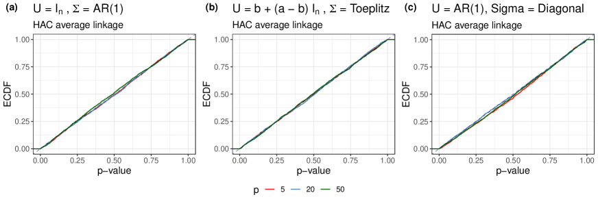
Figure 2: Empirical cumulative distribution functions (ECDF) of $p$-values (2) with $\mathcal{C}$ being a hierarchical clustering algorithm with average linkage. The ECDF were computed from $M=2000$ realizations of (2) under the three dependence settings $(a)$, $(b)$ and $(c)$ with $\boldsymbol{\mu}=\mathbf{0}_{n\times p}$, $n=100$ and $p\in\{5,20,50\}$.

Super-uniform $p$-values for unknown $\mathbf{\Sigma}$

In this section, we illustrate that $p$-values (25) are asymptotically super-uniform when $\Sigma$ is asymptotically over-estimated in the sens of Loewner partial order, as proved in Theorem 3.1. We use the estimator (28) that asymptotically over-estimates $\mathbf{\Sigma}$ if Assumptions 3.1, 3.2 and 3.3 hold. This is indeed the case for the three dependence scenarios $(a)$, $(b)$ and $(c)$, following Remarks 3.1, 3.2 and 3.3 respectively. The estimate is computed using an independent and identically distributed copy of the sample where the clustering was performed, following Proposition 3.4.

We follow the same steps as in [16, Section D.1]. For $n=500$ and $p=10$, we simulate $M=5000$ samples drawn from (2) in settings $(a)$, $(b)$ and $(c)$ with $\boldsymbol{\mu}$ being divided into two clusters:

$$\mu_{ij}=\begin{cases}\frac{\delta}{j}&\mathrm{if}\,\,i\leq\frac{n}{2},\\ -\frac{\delta}{j}&\mathrm{otherwise},\end{cases}\quad\forall\,i\in\{1,\ldots,n\},\,\forall\,j\in\{1,\ldots,p\},$$ (50)

with $\delta\in\{4,6\}$. For $k$-means and HAC with average, centroid, single and complete linkage we set $\mathcal{C}$ to chose three clusters. The samples for which (5) held when comparing two randomly selected clusters are kept. Results for HAC with average linkage are presented in Figure 3. The results for $k$-means and HAC with centroid, single and complete linkage are analogous and we present them in Appendix D.3. All simulations illustrate the asymptotic super-uniformity of $p$-values (2) under the null hypothesis, when $\mathbf{\Sigma}$ is asymptotically over-estimated using (28). Moreover, as the distance between clusters $\delta$ decreases, the over-estimation is less severe and the null distribution of $p$-values approaches the one of a uniform random variable.

It is important to remark that Figure 3 serves only to illustrate the validity of Theorem 3.1, but in no way to interpret the conservativeness of $p$-values when $\mathbf{\Sigma}$ is over-estimated. The deviation from uniformity of the null distribution of (25) or, equivalently, the power of the corresponding test, depends on the measure of the conditioning set, which in Figure 3 is determined by the frequency of iterations satisfying (5).

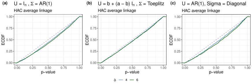
Figure 3: Empirical cumulative distribution functions (ECDF) of $p$-values (2) with $\mathcal{C}$ being a hierarchical clustering algorithm with average linkage. The ECDF are computed from $M=5000$ realizations of (2) under the three dependence settings $(a)$, $(b)$ and $(c)$ with $n=500$, $p=10$ and $\boldsymbol{\mu}$ given by (50) with $\delta\in\{4,6\}$. Only samples for which the null hypothesis held were kept, as described in Section 5.2.

Power analysis

We conclude the numerical simulations on synthetic data by assessing the relative efficiency of the five clustering algorithms considered in terms of power. As in [16, Section 5.2], we consider the conditional power of the $p$-value (2), which is the probability of rejecting the null (5) for a randomly selected pair of clusters when it holds. To estimate the conditional power, we simulate $M=5000$ samples drawn from (2) under the three settings $(a)$, $(b)$ and $(c)$ with $\boldsymbol{\mu}$ dividing the $n=50$ observations into three true clusters:

$$\mu_{ij}=\begin{cases}-\frac{\delta}{2}&\mathrm{if}\,\,i\leq\lfloor\frac{n}{3}\rfloor,\\ \frac{\sqrt{3}\delta}{2}&\mathrm{if}\,\,\lfloor\frac{n}{3}\rfloor<i\leq\lfloor\frac{2n}{3}\rfloor,\\ \frac{\delta}{2}&\mathrm{otherwise},\end{cases}\quad\forall\,i\in\{1,\ldots,n\},\,\forall\,j\in\{1,\ldots,p\},$$ (51)

for $p=10$ and for $14$ evenly-spaced values of $\delta\in[4,10.5]$. Then, we estimate the conditional power as the proportion of rejections at level $\alpha=0.05$ among the samples for which the null hypothesis (5) did not hold (which were above the 90% of $n$ in all settings). The conditional power as a function of $\delta$ is shown in Figure 4 for the three scenarios $(a)$, $(b)$ and $(c)$ and the five considered clustering algorithms. The $p$-values for HAC with complete linkage are estimated using the approximation (22) with $N=2000$ iterations.

Figure 4 shows that, in all cases, conditional power increases with the distance between true clusters. Regarding HAC, we observe that average linkage presents the best relative efficiency among the four considered linkages in all the dependence settings, followed closely by complete linkage, which seems to weaken in $(b)$. This might suggest that conditional power depends on the scale matrices and some scenarios might strongly differ from the overall observed behavior. Indeed, the qualitative difference between average or complete linkage and centroid or single linkage that is observed in $(a)$ and $(c)$ considerably lessens in $(b)$. In $(a)$ and $(c)$, the performance of single linkage is undoubtedly the lowest, and large differences between clusters are required to attain satisfactory levels of conditional power. However, single linkage achieves the second best performance in $(b)$.

The relative efficiency of the $k$-means algorithm in terms of conditional power is one of the worst among all the considered algorithms. This behavior was already pointed out by the authors in [9], who referred to the fact that conditioning on too much information entails a loss of power [20, 25, 8, 15]. Recall that the truncation set for $k$-means post-clustering inference defined in [8] is non-maximal to allow its efficient computation (see Section 4 and [9, Equation (9)]). This approach, although respecting the selective type I error as shown in Theorem 4.1, sacrifices the efficiency in terms of power of the corresponding test, as illustrated in Figure 4.

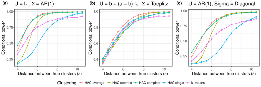
Figure 4: Conditional power for the test proposed in Section 2 under model (2) with the three dependence settings $(a)$, $(b)$ and $(c)$ and the mean matrix defined in (51). The conditional power is estimated as the proportion of rejection at level $\alpha=0.05$ among the subset of the $M=5000$ realizations of (2) for which the null hypothesis (5) holds.

Application to clustering of protein structures

Proteins are essential molecules in all living organisms. Many of their numerous functions are closely related to their non-static structure, which exhibits high variability within numerous protein families [24, 14, 30]. The characterization of such intrinsic structural complexity represents a highly active area of research in the field of Structural Biology. In this pursuit, clustering methods applied to protein conformations have provided valuable insights into this challenging problem [10, 3]. One of the most commonly-chosen descriptors to characterize a protein conformation is the set of pairwise Euclidean distances between every pair of amino acids along the sequence [33, 28, 22], usually referred to as distance maps. As these distances are strongly correlated, assuming a constant diagonal covariance matrix as in [16] seems very unrealistic. Instead, we opt for the more convenient model

$$\mathbf{X}\sim\mathcal{MN}_{n\times p}(\boldsymbol{\mu},\mathbf{I}_{n},\mathbf{\Sigma}),$$ (52)

where $\mathbf{\Sigma}$ can be estimated using (28). Each row of $\mathbf{X}$ corresponds to a protein conformation, featured by a vector of Euclidean distances between every pair of amino acids, which constitute the columns of $\mathbf{X}$. We perform hierarchical agglomerative clustering with average linkage (as it showed the best relative efficiency in Section 5.3) to estimate $k=6$ clusters among $n=2000$ conformations of a disordered protein called Histatin-5 (Hst5). The number of clusters was chosen arbitrarily. The corresponding sequence is 24 amino acids long, so $p=23\cdot 24/2=276$. The conformations were generated using Flexible-Meccano [31, 6] and refined using previously reported small-angle X-ray scattering (SAXS) data [35]. Note that Flexible-Meccano is a sampling algorithm that generates an independent conformation at each iteration, contrary to Molecular Dynamics simulation techniques that present temporal dependence between samples. This justifies our choice of $\mathbf{U}=\mathbf{I}_{n}$. Moreover, we had access to an independent replica of the simulated ensemble that we used to estimate $\mathbf{\Sigma}$, as it is usual for generated protein ensembles. Figure 5 shows the average distance map across all conformations in a given cluster or, in other words, the empirical cluster means $\bar{X}_{\hat{C}_{1}},\ldots,\bar{X}_{\hat{C}_{6}}$ as defined in (4). Table 1 presents the $p$-values corresponding to every pair of clusters, corrected for multiple testing using the Bonferroni-Holm adjustment [18].

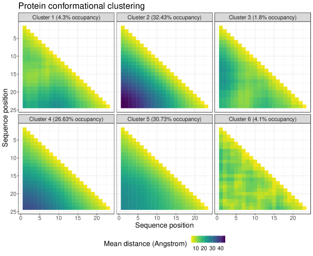
Figure 5: Average pairwise distances between every pair of amino acids across the conformations of each cluster. The clusters were found after performing hierarchical clustering with average linkage on the protein data presented in Section 6.

Cluster	1	2	3	4	5
2	2.187589$\cdot 10^{-4}$
3	3.039844$\cdot 10^{-11}$	1.41$\cdot 10^{-3}$
4	1.070993$\cdot 10^{-10}$	0.300540	2.98464$\cdot 10^{-4}$
5	3.038979$\cdot 10^{-16}$	0.093018	6.015797$\cdot 10^{-5}$	0.105446
6	1.729616$\cdot 10^{-6}$	0.010612	9.290826$\cdot 10^{-9}$	2.105$\cdot 10^{-3}$	5.624624$\cdot 10^{-5}$

Table 1: $p$-values (2) computed under model (52) retrieved after testing (5) on the protein data presented in Section 6. The hierarchical clustering algorithm was set to find six clusters using average linkage. In blue, adjusted $p$-values for which the null is not rejected at level $\alpha=0.05$.

The $p$-values presented in Table 1 show significant differences between the most part of the average distance maps depicted in Figure 5. The non-rejecting pairs of clusters at level $\alpha=0.05$, marked in blue in Table 1, suggest that clusters 2, 4 and 5 could be merged into a single group. Indeed, when looking at the corresponding empirical means $\bar{X}_{\hat{C}_{2}}$, $\bar{X}_{\hat{C}_{4}}$ in Figure 5, we appreciate that these three clusters are characterized by large distances between pairs of amino acids that are far apart in the sequence, which indicates a lack of interactions between the sequence termini and a more extended structure of the corresponding conformations. This feature appears as an exclusive and prominent characteristic of clusters 2, 4 and 5, which might explain the non-rejection of the corresponding nulls. For the rest of rejecting pairs of clusters, clear differences in distance patterns are retrieved in Figure 5, accounting for significant changes on Hst5 structure between the corresponding groups. The results presented in Table 1 are coherent with the HAC dendrogram, presented in Figure 6, showing that clusters 2, 4, and 5 form a subgroup that is promptly separated from the rest.

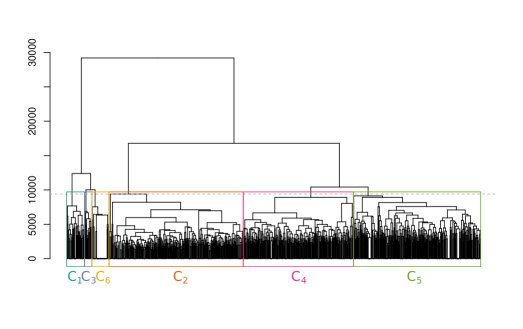
Figure 6: HAC dendrogram for the Hst5 protein ensemble data, with the six estimated clusters marked with colored rectangles.

Discussion

The seminal work by Gao et al. [16] has laid the foundation for selective inference after clustering by introducing the theoretical framework allowing to test differences between cluster means, conditioning on having estimated those clusters. Furthermore, the authors have tackled the problem of estimating unknown parameters while controlling the selective type I error, which had been overlooked in previous works [23, 34], but which is crucial for the practical application of this theory. Their contribution motivates extensions of post-clustering inference to more general frameworks that arise in complex real applications, where observations or features present non-negligible dependence structures. In this work, we generalize the model considered in [16] to non-independent observations and features, as well as the adequate estimation of the dependence structure, from the uni-dimensional case in [16] to the matrix framework presented here. These extensions, presented in Sections 2 and 3 respectively, and numerically illustrated in Sections 5 and 6, represent the main contributions of this work.

The theoretical framework presented in Section 2 covers any known dependence structure for observations and features. The main idea is to replace the Euclidean norm in [16] by the Mahalanobis distance with respect to the null distribution of the difference of means (9) to define the test statistic (Theorem 2.1). This removes the information about the variance from the statistic null distribution, which becomes independent of $\mathbf{U}$ and $\mathbf{\Sigma}$. Although the joint estimation of both scale matrices $\mathbf{\Sigma}$ and $\mathbf{U}$ is difficult to manage under (2), we have set the framework allowing the estimation of one of them when the other one is known. The key idea is to redefine the asymptotic over-estimation in terms of the Loewner partial order, which maintains the asymptotic control of the selective type I error (Theorem 3.1). Following Proposition 3.4, an i.i.d. copy of $\mathbf{X}$ is required to estimate $\mathbf{\Sigma}$. Resorting to data splitting here is unfeasible if $\mathbf{U}$ is not block diagonal with identical blocks. Several copies of $\mathbf{X}$ are naturally available in some applications, as is the case in the analysis of simulated protein ensembles presented in Section 6. To allow valid post-clustering inference in real scenarios, we provide an estimator of $\mathbf{\Sigma}$ that asymptotically over-estimates $\mathbf{\Sigma}$ when $\mathbf{U}$ satisfies Assumptions 3.1, 3.2 and 3.3. Future work could focus on showing that these assumptions are satisfied for new models of dependence between observations, besides the one presented in Remarks 3.1, 3.2 and 3.3.

Clustering is a multidimensional method that incorporates information from $p$ descriptors to classify $n$ observations. However, the estimated groups are often distinguished by a subset of variables, whose determination is essential in various fields of application [29, 39]. The framework presented in [16] has been adapted to feature-level post-clustering inference in [17], testing for the difference of the $g$-th coordinate of cluster means, for a fixed $g\in\{1,\ldots,p\}$. In that case, clustering is performed on the complete data set $\mathbf{X}$ but inference is carried out on the $g$-th column, modeled by a $n$-dimensional Gaussian of covariance matrix $\sigma_{g}^{2}\mathbf{I}_{n}$, for a $\sigma_{g}>0$. Note that the possible dependence structure between features is not taken into account for inference, but only the covariance between observations. Following a similar reasoning as in [16], the authors in [17] define a $p$-value that controls the selective type I error. However, no efficient analytic computation is not proposed, and a Monte Carlo approximation is used. Following the strategy presented here, adapting the framework of [17] to arbitrary dependence between observations is straightforward, but it would entail the same limitations regarding the efficient computation of the $p$-value. The analytical determination of the truncation set in that framework would be an important contribution. Additionally, the non-trivial extension of the over-estimation strategy presented in Section 3 to this framework would be essential to allow the practical implementation of the feature-level selective test.

Another potential avenue for exploration is the adaptation of the efficient computation of the truncation set, as presented in [16, 9], to other clustering algorithms. The combination of dimension reduction algorithms, such as t-SNE [38] and UMAP [27], with clustering techniques has gained immense popularity in various fields of Biology due to its remarkable empirical efficiency [10, 11, 3, 12, 5, 1]. As such, it would be useful to develop methods that avoid computationally expensive Monte Carlo approximations and efficiently compute the truncation set in scenarios where, for example, $\mathcal{C}$ represents the composition of a dimension reduction algorithm with hierarchical or $k$-means clustering.

As discussed in Section 4, performing analytically tractable post-clustering inference requires the addition of technical events to the conditioning set, which implies a reduction in power. Investigating whether these conditions might be relaxed is an interesting path for future research. The problem of power loss due to extra conditioning is not exclusive to this method. Techniques like data fission [23] need to calibrate the conditioning information and consequences in terms of power are analogous. However, it is still unknown whether power loss is more drastic in one method or the other. An interesting contribution would be to establish a framework allowing for a proper comparison of this effect when performing post-clustering inference using data fission and the approach proposed in [16]. Nevertheless, extending this comparison to practical applications would be unfeasible as long as the estimation of the covariance structure with statistical guarantees cannot be carried out in both methods.

Code availability

The methods introduced in the present work were implemented in the R package PCIdep, available at https://github.com/gonzalez-delgado/PCIdep. The package makes use of the R package clusterpval, providing the approaches of [16], and the R package KmeansInference, providing the approaches of [9].

Appendix A Proofs of Section 2

Proof of Theorem 2.1.

We follow the steps of the proof of Theorem 1 in [16]. We begin by deriving the null distribution of the test statistic $\left\lVert\bar{X}_{\mathcal{G}_{1}}-\bar{X}_{\mathcal{G}_{2}}\right\rVert_{\mathbf{V}_{\mathcal{G}_{1},\mathcal{G}_{2}}}$ under the null $H_{0}^{\{\mathcal{G}_{1},\mathcal{G}_{2}\}}$. First, we have

$$\mathbf{X}\sim\mathcal{M}\mathcal{N}_{n\times p}(\boldsymbol{\mu},\mathbf{U},\mathbf{\Sigma})\Leftrightarrow\mathbf{X}^{T}\sim\mathcal{M}\mathcal{N}_{p\times n}(\boldsymbol{\mu}^{T},\mathbf{\Sigma},\mathbf{U})\Leftrightarrow\mathrm{vec}(\mathbf{X}^{T})\sim\mathcal{N}_{np}(\mathrm{vec}(\boldsymbol{\mu}^{T}),\mathbf{U}\otimes\mathbf{\Sigma}),$$ (53)

where $\mathrm{vec}(\mathbf{X}^{T})$ is a column vector concatenating the $n$ vectors of $p$-dimensional observations that constitute $\mathbf{X}$. If we restrict $\mathrm{vec}(\mathbf{X}^{T})$ to the observations (10) in $\mathcal{G}_{1}\cup\mathcal{G}_{2}$ , we have

$$X_{\mathcal{G}_{1},\mathcal{G}_{2}}\sim\mathcal{N}_{p(\left\lvert\mathcal{G}_{1}\right\rvert+\left\lvert\mathcal{G}_{2}\right\rvert)}(\bar{\mu}_{\mathcal{G}_{1},\mathcal{G}_{2}},\mathbf{U}_{\mathcal{G}_{1},\mathcal{G}_{2}}\otimes\mathbf{\Sigma})$$ (54)

where $\bar{\mu}_{\mathcal{G}_{1},\mathcal{G}_{2}}=(\mathrm{vec}(\bar{\mu}_{\mathcal{G}_{1}}^{T}),\mathrm{vec}(\bar{\mu}_{\mathcal{G}_{2}}^{T}))$. Then, we can apply the linear transformation $\mathbf{D}_{\mathcal{G}_{1},\mathcal{G}_{2}}$ (11) to obtain the difference of means and get

$$\bar{X}_{\mathcal{G}_{1}}-\bar{X}_{\mathcal{G}_{2}}=\mathbf{D}_{\mathcal{G}_{1},\mathcal{G}_{2}}X_{\mathcal{G}_{1},\mathcal{G}_{2}}\sim\mathcal{N}_{p}\left(\bar{\mu}_{\mathcal{G}_{1}}-\bar{\mu}_{\mathcal{G}_{2}},\mathbf{D}_{\mathcal{G}_{1},\mathcal{G}_{2}}(\mathbf{U}_{\mathcal{G}_{1},\mathcal{G}_{2}}\otimes\mathbf{\Sigma})\mathbf{D}_{\mathcal{G}_{1},\mathcal{G}_{2}}^{T}\right),$$ (55)

that, under $H_{0}^{\{\mathcal{G}_{1},\mathcal{G}_{2}\}}$, gives

$$\bar{X}_{\mathcal{G}_{1}}-\bar{X}_{\mathcal{G}_{2}}\overset{H_{0}^{\{\mathcal{G}_{1},\mathcal{G}_{2}\}}}{\sim}\mathcal{N}_{p}\left(0,\mathbf{V}_{\mathcal{G}_{1},\mathcal{G}_{2}}\right),$$ (56)

where we replaced $\mathbf{V}_{\mathcal{G}_{1},\mathcal{G}_{2}}$ by its definition (12). $\mathbf{U}_{\mathcal{G}_{1},\mathcal{G}_{2}}$ is positive definite as it is a principal submatrix of $\mathbf{U}$. The Kronecker product of two positive definite matrices is also positive definite and, as $\mathbf{D}_{\mathcal{G}_{1},\mathcal{G}_{2}}$ is a full rank linear operator, $\mathbf{V}_{\mathcal{G}_{1},\mathcal{G}_{2}}$ is positive definite [19, Observation 7.1.8]. Consequently, $\mathbf{V}_{\mathcal{G}_{1},\mathcal{G}_{2}}$ is invertible and defines the norm (9) in $\mathbb{R}^{p}$. This, together with (56), yields

$$\left\lVert\bar{X}_{\mathcal{G}_{1}}-\bar{X}_{\mathcal{G}_{2}}\right\rVert_{\mathbf{V}_{\mathcal{G}_{1},\mathcal{G}_{2}}}^{2}\overset{H_{0}^{\{\mathcal{G}_{1},\mathcal{G}_{2}\}}}{\sim}\chi_{p}^{2}.$$ (57)

Let us now build the $p$-value for $H_{0}^{\{\mathcal{G}_{1},\mathcal{G}_{2}\}}$, by slightly adapting the reasoning in [16]. On one hand, for any $\nu\in\mathbb{R}^{n}$, we have

$$\mathbf{X}=\boldsymbol{\pi}_{\nu}^{\perp}\mathbf{X}+(\mathbf{I}_{n}-\boldsymbol{\pi}_{\nu}^{\perp}\mathbf{X})=\boldsymbol{\pi}_{\nu}^{\perp}\mathbf{X}+\left(\frac{\left\lVert\mathbf{X}^{T}\nu\right\rVert_{\mathbf{V}_{\mathcal{G}_{1},\mathcal{G}_{2}}}}{\left\lVert\nu\right\rVert_{2}^{2}}\right)\nu\,\mathrm{dir}_{\mathbf{V}_{\mathcal{G}_{1},\mathcal{G}_{2}}}(\mathbf{X}^{T}\nu)^{T}.$$ (58)

Following (8), $\mathbf{X}^{T}\nu(\mathcal{G}_{1},\mathcal{G}_{2})=\bar{X}_{\mathcal{G}_{1}}-\bar{X}_{\mathcal{G}_{2}}$ and $\left\lVert\nu(\mathcal{G}_{1},\mathcal{G}_{2})\right\rVert_{2}^{2}=1/\left\lvert\mathcal{G}_{1}\right\rvert+1/\left\lvert\mathcal{G}_{2}\right\rvert$. Thus, we can write

$$\mathbf{X}=\boldsymbol{\pi}_{\nu}(\mathcal{G}_{1},\mathcal{G}_{2})^{\perp}\mathbf{X}+\left(\frac{\left\lVert\bar{X}_{\mathcal{G}_{1}}-\bar{X}_{\mathcal{G}_{2}}\right\rVert_{\mathbf{V}_{\mathcal{G}_{1},\mathcal{G}_{2}}}}{\frac{1}{\left\lvert\mathcal{G}_{1}\right\rvert}+\frac{1}{\left\lvert\mathcal{G}_{2}\right\rvert}}\right)\nu(\mathcal{G}_{1},\mathcal{G}_{2})\,\mathrm{dir}_{\mathbf{V}_{\mathcal{G}_{1},\mathcal{G}_{2}}}(\bar{X}_{\mathcal{G}_{1}}-\bar{X}_{\mathcal{G}_{2}})^{T}.$$ (59)

On the other hand, from the proof in [16] we have $\boldsymbol{\pi}_{\nu}(\mathcal{G}_{1},\mathcal{G}_{2})^{\perp}\mathbf{X}\mathchoice{\mathrel{\hbox to0.0pt{$\displaystyle\perp$\hss}\mkern 2.0mu{\displaystyle\perp}}}{\mathrel{\hbox to0.0pt{$\textstyle\perp$\hss}\mkern 2.0mu{\textstyle\perp}}}{\mathrel{\hbox to0.0pt{$\scriptstyle\perp$\hss}\mkern 2.0mu{\scriptstyle\perp}}}{\mathrel{\hbox to0.0pt{$\scriptscriptstyle\perp$\hss}\mkern 2.0mu{\scriptscriptstyle\perp}}}\mathbf{X}^{T}\nu(\mathcal{G}_{1},\mathcal{G}_{2})$, which implies

$$\left\lVert\bar{X}_{\mathcal{G}_{1}}-\bar{X}_{\mathcal{G}_{2}}\right\rVert_{\mathbf{V}_{\mathcal{G}_{1},\mathcal{G}_{2}}}\mathchoice{\mathrel{\hbox to0.0pt{$\displaystyle\perp$\hss}\mkern 2.0mu{\displaystyle\perp}}}{\mathrel{\hbox to0.0pt{$\textstyle\perp$\hss}\mkern 2.0mu{\textstyle\perp}}}{\mathrel{\hbox to0.0pt{$\scriptstyle\perp$\hss}\mkern 2.0mu{\scriptstyle\perp}}}{\mathrel{\hbox to0.0pt{$\scriptscriptstyle\perp$\hss}\mkern 2.0mu{\scriptscriptstyle\perp}}}\boldsymbol{\pi}_{\nu}(\mathcal{G}_{1},\mathcal{G}_{2})^{\perp}\mathbf{X}$$ (60)

and, from the independence of the length and direction (in any norm) of a centered multivariate normal vector (56), we have

$$\left\lVert\bar{X}_{\mathcal{G}_{1}}-\bar{X}_{\mathcal{G}_{2}}\right\rVert_{\mathbf{V}_{\mathcal{G}_{1},\mathcal{G}_{2}}}\mathchoice{\mathrel{\hbox to0.0pt{$\displaystyle\perp$\hss}\mkern 2.0mu{\displaystyle\perp}}}{\mathrel{\hbox to0.0pt{$\textstyle\perp$\hss}\mkern 2.0mu{\textstyle\perp}}}{\mathrel{\hbox to0.0pt{$\scriptstyle\perp$\hss}\mkern 2.0mu{\scriptstyle\perp}}}{\mathrel{\hbox to0.0pt{$\scriptscriptstyle\perp$\hss}\mkern 2.0mu{\scriptscriptstyle\perp}}}\mathrm{dir}_{\mathbf{V}_{\mathcal{G}_{1},\mathcal{G}_{2}}}(\bar{X}_{\mathcal{G}_{1}}-\bar{X}_{\mathcal{G}_{2}}).$$ (61)

We can now plug (59) in the definition of our $p$-value (2) and, applying (60) and (61), we can derive

$$p_{\mathbf{V}_{\mathcal{G}_{1},\mathcal{G}_{2}}}(\mathbf{x};\{\mathcal{G}_{1},\mathcal{G}_{2}\})=\mathbb{P}_{H_{0}^{\{\mathcal{G}_{1},\mathcal{G}_{2}\}}}\left(\left\lVert\bar{X}_{\mathcal{G}_{1}}-\bar{X}_{\mathcal{G}_{2}}\right\rVert_{\mathbf{V}_{\mathcal{G}_{1},\mathcal{G}_{2}}}\geq\left\lVert\bar{x}_{\mathcal{G}_{1}}-\bar{x}_{\mathcal{G}_{2}}\right\rVert_{\mathbf{V}_{\mathcal{G}_{1},\mathcal{G}_{2}}}\,\,\right.\biggr{\rvert}$$

$$\left.\left\lVert\bar{X}_{\mathcal{G}_{1}}-\bar{X}_{\mathcal{G}_{2}}\right\rVert_{\mathbf{V}_{\mathcal{G}_{1},\mathcal{G}_{2}}}\in\,\mathcal{S}_{\mathbf{V}_{\mathcal{G}_{1},\mathcal{G}_{2}}}(\mathbf{x};\{\mathcal{G}_{1},\mathcal{G}_{2}\})\right),$$ (62)

where the set $\mathcal{S}_{\mathbf{V}_{\mathcal{G}_{1},\mathcal{G}_{2}}}(\mathbf{x};\{\mathcal{G}_{1},\mathcal{G}_{2}\})$ is defined in (15). Consequently, if we denote by $\mathbb{F}_{p}(t,\mathcal{S})$ the cumulative distribution function of a $\chi_{p}$ random variable truncated to the set $\mathcal{S}$, from (A) and (57) we have

$$p_{\mathbf{V}_{\mathcal{G}_{1},\mathcal{G}_{2}}}(\mathbf{x};\{\mathcal{G}_{1},\mathcal{G}_{2}\})=1-\mathbb{F}_{p}\left(\left\lVert\bar{x}_{\mathcal{G}_{1}}-\bar{x}_{\mathcal{G}_{2}}\right\rVert_{\mathbf{V}_{\mathcal{G}_{1},\mathcal{G}_{2}}}\,,\,\mathcal{S}_{\mathbf{V}_{\mathcal{G}_{1},\mathcal{G}_{2}}}(\mathbf{x};\{\mathcal{G}_{1},\mathcal{G}_{2}\})\right),$$ (63)

which proves the first statement (14). The control of selective type I error is proved identically to the reasoning in the proof of [16, Theorem 1]. ∎

Proof of Lemma 2.2.

Let us first show that the perturbed data sets $\mathbf{x}^{\prime}(\phi)$, defined in [16, Equation (13)] and $\mathbf{x}^{\prime}_{\mathbf{V}_{\hat{C}_{1},\hat{C}_{2}}}(\phi)$, defined in (17) are the same up to a scale transformation, i.e. that

$$\mathbf{x}^{\prime}_{\mathbf{V}_{\hat{C}_{1},\hat{C}_{2}}}(\phi)=\mathbf{x}^{\prime}\left(\frac{\left\lVert\bar{x}_{\hat{C}_{1}}-\bar{x}_{\hat{C}_{2}}\right\rVert_{2}}{\left\lVert\bar{x}_{\hat{C}_{1}}-\bar{x}_{\hat{C}_{2}}\right\rVert_{\mathbf{V}_{\hat{C}_{1},\hat{C}_{2}}}}\,\phi\right)\quad\forall\,\phi\geq 0.$$ (64)

Note first that we can write

$$\left(\frac{\left\lVert\bar{x}_{\hat{C}_{1}}-\bar{x}_{\hat{C}_{2}}\right\rVert_{2}}{\left\lVert\bar{x}_{\hat{C}_{1}}-\bar{x}_{\hat{C}_{2}}\right\rVert_{\mathbf{V}_{\hat{C}_{1},\hat{C}_{2}}}}\,\phi-\left\lVert\bar{x}_{\hat{C}_{1}}-\bar{x}_{\hat{C}_{2}}\right\rVert_{2}\right)\mathrm{dir}(\bar{x}_{\hat{C}_{1}}-\bar{x}_{\hat{C}_{2}})=\left(\phi-\left\lVert\bar{x}_{\hat{C}_{1}}-\bar{x}_{\hat{C}_{2}}\right\rVert_{\mathbf{V}_{\hat{C}_{1},\hat{C}_{2}}}\right)\mathrm{dir}_{\mathbf{V}_{\hat{C}_{1},\hat{C}_{2}}}(\bar{x}_{\hat{C}_{1}}-\bar{x}_{\hat{C}_{2}}),$$ (65)

where $\mathrm{dir}(u)=u/\left\lVert u\right\rVert_{2}\mathds{1}\{u\neq 0\}$. Replacing (65) in (19), we have (64). Finally, it suffices to remark that

$$\hat{\mathcal{S}}_{\mathbf{V}_{\hat{C}_{1},\hat{C}_{2}}}=\left\{\phi\geq 0\,:\,\hat{C}_{1},\hat{C}_{2}\in\mathcal{C}\left(\mathbf{x}^{\prime}_{\mathbf{V}_{\hat{C}_{1},\hat{C}_{2}}}(\phi)\right)\right\}=\left\{\phi\geq 0\,:\,\hat{C}_{1},\hat{C}_{2}\in\mathcal{C}\left(\mathbf{x}^{\prime}\left(\frac{\left\lVert\bar{x}_{\hat{C}_{1}}-\bar{x}_{\hat{C}_{2}}\right\rVert_{2}}{\left\lVert\bar{x}_{\hat{C}_{1}}-\bar{x}_{\hat{C}_{2}}\right\rVert_{\mathbf{V}_{\hat{C}_{1},\hat{C}_{2}}}}\,\phi\right)\right)\right\}$$

$$=\left\{\frac{\left\lVert\bar{x}_{\hat{C}_{1}}-\bar{x}_{\hat{C}_{2}}\right\rVert_{\mathbf{V}_{\hat{C}_{1},\hat{C}_{2}}}}{\left\lVert\bar{x}_{\hat{C}_{1}}-\bar{x}_{\hat{C}_{2}}\right\rVert_{2}}\,\phi\,:\,\hat{C}_{1},\hat{C}_{2}\in\mathcal{C}(\mathbf{x}^{\prime}(\phi))\right\}=\frac{\left\lVert\bar{x}_{\hat{C}_{1}}-\bar{x}_{\hat{C}_{2}}\right\rVert_{\mathbf{V}_{\hat{C}_{1},\hat{C}_{2}}}}{\left\lVert\bar{x}_{\hat{C}_{1}}-\bar{x}_{\hat{C}_{2}}\right\rVert_{2}}\,\hat{\mathcal{S}},$$

which concludes the proof. ∎

Appendix B Proofs of Section 3

Proof of Theorem 3.1.

We follows the steps of the proof of Theorem 4 in [16]. For simplicity, we use $\hat{p}_{n}$ to denote $p_{\hat{\mathbf{V}}_{\hat{C}_{1}^{(n)},\hat{C}_{2}^{(n)}}}\left(\mathbf{X}^{(n)};\left\{\hat{C}_{1}^{(n)},\hat{C}_{2}^{(n)}\right\}\right)$, $p_{n}$ to denote $p_{\mathbf{V}_{\hat{C}_{1}^{(n)},\hat{C}_{2}^{(n)}}}\left(\mathbf{X}^{(n)};\left\{\hat{C}_{1}^{(n)},\hat{C}_{2}^{(n)}\right\}\right)$, $\hat{\mathbf{V}}_{n}$ to denote $\hat{\mathbf{V}}_{\hat{C}_{1}^{(n)},\hat{C}_{2}^{(n)}}$ and $\mathbf{V}_{n}$ to denote $\mathbf{V}_{\hat{C}_{1}^{(n)},\hat{C}_{2}^{(n)}}$. If we show that

$$\hat{\mathbf{\Sigma}}\left(\mathbf{X}^{(n)}\right)\succeq\mathbf{\Sigma}\,\Rightarrow\,\hat{p}_{n}\geq p_{n},$$ (66)

then the result follows using the same reasoning as in the proof of [16, Theorem 4], replacing the usual order $\geq$ in $\mathbb{R}$ by the Loewner partial order $\succeq$ between matrices. Consequently, we only need to prove (66). First note that, as the Kronecker product is distributive, we have

$$\hat{\mathbf{\Sigma}}\left(\mathbf{X}^{(n)}\right)\succeq\mathbf{\Sigma}\,\Rightarrow\,\hat{\mathbf{V}}_{n}\succeq\mathbf{V}_{n}.$$ (67)

Next, by Corollary 7.7.4(a) and Theorem 7.7.2(a) in [19], we can write

$$\hat{\mathbf{V}}_{n}\succeq\mathbf{V}_{n}\,\Leftrightarrow\,\mathbf{V}_{n}^{-1}\succeq\hat{\mathbf{V}}_{n}^{-1}$$

$$\Rightarrow\left(\overline{X^{(n)}}_{\hat{C}_{1}^{(n)}}-\overline{X^{(n)}}_{\hat{C}_{2}^{(n)}}\right)^{T}\,\mathbf{V}^{-1}_{n}\,\left(\overline{X^{(n)}}_{\hat{C}_{1}^{(n)}}-\overline{X^{(n)}}_{\hat{C}_{2}^{(n)}}\right)$$

$$\geq\left(\overline{X^{(n)}}_{\hat{C}_{1}^{(n)}}-\overline{X^{(n)}}_{\hat{C}_{2}^{(n)}}\right)^{T}\,\hat{\mathbf{V}}^{-1}_{n}\,\left(\overline{X^{(n)}}_{\hat{C}_{1}^{(n)}}-\overline{X^{(n)}}_{\hat{C}_{2}^{(n)}}\right)$$

$$\Leftrightarrow\left\lVert\overline{X^{(n)}}_{\hat{C}_{1}^{(n)}}-\overline{X^{(n)}}_{\hat{C}_{2}^{(n)}}\right\rVert_{\mathbf{V}_{n}}\geq\left\lVert\overline{X^{(n)}}_{\hat{C}_{1}^{(n)}}-\overline{X^{(n)}}_{\hat{C}_{2}^{(n)}}\right\rVert_{\hat{\mathbf{V}}_{n}}.$$ (68)

Let us then state that, if $\mathbb{F}_{p}(t,c,\mathcal{S})$ denotes the cumulative distribution function of a $c\cdot\chi_{p}$ distribution truncated to the set $\mathcal{S}$, for $c>0$, it follows that

$$\mathbb{F}_{p}(t,c,a\,\mathcal{S})=\mathbb{F}_{p}\left(\frac{t}{a},\frac{c}{a},\mathcal{S}\right),$$ (69)

for any $a>0$. We prove (69) as a technical lemma after the proof. With a slight abuse of notation we write $\mathbb{F}_{p}(t,1,\mathcal{S})=\mathbb{F}_{p}(t,\mathcal{S})$ where $\mathbb{F}_{p}(t,\mathcal{S})$ is the CDF involved in (14). Consequently, taking

$$a=\frac{\left\lVert\overline{X^{(n)}}_{\hat{C}_{1}^{(n)}}-\overline{X^{(n)}}_{\hat{C}_{2}^{(n)}}\right\rVert_{\hat{\mathbf{V}}_{n}}}{\left\lVert\overline{X^{(n)}}_{\hat{C}_{1}^{(n)}}-\overline{X^{(n)}}_{\hat{C}_{2}^{(n)}}\right\rVert_{\mathbf{V}_{n}}}\leq 1,$$ (70)

we have

$$1-\hat{p}_{n}=\mathbb{F}_{p}\left(\left\lVert\overline{X^{(n)}}_{\hat{C}_{1}^{(n)}}-\overline{X^{(n)}}_{\hat{C}_{2}^{(n)}}\right\rVert_{\hat{\mathbf{V}}_{n}}\,,\,\mathcal{S}_{\hat{\mathbf{V}}_{n}}\right)=\mathbb{F}_{p}\left(\left\lVert\overline{X^{(n)}}_{\hat{C}_{1}^{(n)}}-\overline{X^{(n)}}_{\hat{C}_{2}^{(n)}}\right\rVert_{\hat{\mathbf{V}}_{n}}\,,\,a\,\mathcal{S}_{\mathbf{V}_{n}}\right)$$

$$=\mathbb{F}_{p}\left(\frac{1}{a}\,\left\lVert\overline{X^{(n)}}_{\hat{C}_{1}^{(n)}}-\overline{X^{(n)}}_{\hat{C}_{2}^{(n)}}\right\rVert_{\hat{\mathbf{V}}_{n}}\,,\,\frac{1}{a}\,,\,\mathcal{S}_{\mathbf{V}_{n}}\right)=\mathbb{F}_{p}\left(\left\lVert\overline{X^{(n)}}_{\hat{C}_{1}^{(n)}}-\overline{X^{(n)}}_{\hat{C}_{2}^{(n)}}\right\rVert_{\mathbf{V}_{n}}\,,\,\frac{1}{a}\,,\,\mathcal{S}_{\mathbf{V}_{n}}\right)$$

$$\leq\mathbb{F}_{p}\left(\left\lVert\overline{X^{(n)}}_{\hat{C}_{1}^{(n)}}-\overline{X^{(n)}}_{\hat{C}_{2}^{(n)}}\right\rVert_{\mathbf{V}_{n}}\,,\,1\,,\,\mathcal{S}_{\mathbf{V}_{n}}\right)=1-p_{n},$$ (71)

where the last inequality follows from Lemma A.3 in [16]. This shows (66). ∎

Lemma B.1.

For $c>0$ and $\emptyset\neq\mathcal{S}\subset\mathbb{R}$, let $\mathbb{F}_{p}(t,c,\mathcal{S})$ denote the cumulative distribution function of a $c\cdot\chi_{p}$ distribution truncated to $\mathcal{S}$. Then, for any $a>0$, it holds

$$\mathbb{F}_{p}(t,c,a\,\mathcal{S})=\mathbb{F}_{p}\left(\frac{t}{a},\frac{c}{a},\mathcal{S}\right).$$

Proof of Lemma B.1.

First, if we denote by $f(t,c,\mathcal{S)}$ the probability density function of a $c\cdot\chi_{p}$ distribution truncated to the set $\mathcal{S}$, we have

$$f(t,c,a\,\mathcal{S})=\frac{1}{a}\,f\left(\frac{t}{a},\frac{c}{a},\mathcal{S}\right).$$ (72)

Indeed, following the first lines of the proof of [16, Lemma A.3], we can rewrite $f(t,c,a\,\mathcal{S})$ as

$$f(t,c,a\,\mathcal{S})=\frac{t^{p-1}\,\mathds{1}\{t\in a\,\mathcal{S}\}}{\int u^{p-1}\exp(-\frac{u^{2}}{2c^{2}}),\mathds{1}\{t\in a\,\mathcal{S}\}\,du}\exp\left(-\frac{t^{2}}{2c^{2}}\right),$$ (73)

that we can easily express in terms of $t/a$ as

$$f(t,c,a\,\mathcal{S})=\frac{\left(\frac{t}{a}\right)^{p-1}\,\mathds{1}\{\frac{t}{a}\in\mathcal{S}\}}{\int\left(\frac{u}{a}\right)^{p-1}\exp(-\frac{(u/a)^{2}}{2(c/a)^{2}}),\mathds{1}\{\frac{t}{a}\in\mathcal{S}\}\,du}\exp\left(-\frac{(t/a)^{2}}{2(c/a)^{2}}\right)=\frac{1}{a}\,f\left(\frac{t}{a},\frac{c}{a},\mathcal{S}\right),$$ (74)

where the last equality follows from taking the variable change $y=u/a$ in the integral. Finally, we have

$$\mathbb{F}_{p}(t,c,a\,\mathcal{S})=\int_{0}^{t}f(x,c,a\,\mathcal{S})\,dx=\frac{1}{a}\int_{0}^{t}f\left(\frac{x}{a},\frac{c}{a},\mathcal{S}\right)\,dx=\int_{0}^{\frac{t}{a}}f\left(u,\frac{c}{a},\mathcal{S}\right)\,du\\ =\mathbb{F}_{p}\left(\frac{t}{a},\frac{c}{a},\mathcal{S}\right),$$

which concludes the proof. ∎

Proof of Remark 3.1.

The case of diagonal matrices is straightforward as both $\mathbf{U}^{(n)}$ and $\left(\mathbf{U}^{(n)}\right)^{-1}$ are defined by a sequence $\{\lambda_{i}\}_{i\in\mathbb{N}}$. Every diagonal entry of the inverse satisfies $\left(U^{(n)}\right)^{-1}_{ii}=\frac{1}{\lambda_{i}}$ for all $n\in\mathbb{N}$ and, as we asked the $\lambda_{i}$ to converge to $\lambda$, which is strictly positive due to the positive definiteness of $\mathbf{U}^{(n)}$, Assumption 3.3 is satisfied. ∎

Proof of Remark 3.2.

Let $\mathbf{U}^{(n)}=b\mathbf{1}_{n\times n}+(a-b)\,\mathbf{I}_{n}$. Note that, as $\mathbf{U}^{(n)}$ is positive definite, the coefficients $a,b$ verify $a>b$. This follows the fact that $\max_{i,j}|A_{ij}|\leq\max_{ii}A_{ii}$ for any positive definite matrix $A$. Following the Sherman–Morrison formula [4], we can derive an explicit expression for the sequence of inverse matrices:

$$\left(\mathbf{U}^{(n)}\right)^{-1}=\frac{1}{a-b}\,\mathbf{I}_{n}+\frac{-b}{(a-b)(nb+a-b)},\quad\forall\,n\in\mathbb{N}.$$ (75)

Consequently, for every $r\geq 0$ and every $i\in\mathbb{N}$, we have

$$\left(\mathbf{U}^{(n)}\right)^{-1}_{i\,i+r}=\begin{cases}\frac{1}{a-b}+\frac{-b}{(a-b)(nb+a-b)}&\mathrm{if}\,\,r=0,\\ \frac{-b}{(a-b)(nb+a-b)}&\mathrm{if}\,\,r>0,\end{cases}$$

which are monotone, so condition $(ii)$ in Assumption 3.3 is satisfied. Then, we have

$$\Lambda_{i\,i+r}=\begin{cases}\frac{1}{a-b}&\mathrm{if}\,\,r=0,\\ 0&\mathrm{if}\,\,r>0,\end{cases}$$

for all $i\in\mathbb{N}$, $\lambda_{0}=1/(a-b)$ and $\lambda_{r}=0$ for $r>0$. Consequently, Assumption 3.3 holds. ∎

Proof of Remark 3.3.

The inverse of an auto-regressive covariance matrix of lag $P\geq 1$ is banded with $2P-1$ non-zero diagonals. Its explicit form is derived in [40] for a stationary process of any lag, and the cases $P\leq 3$ are discussed in detail in [41]. From these results we can derive the behavior of the sequences $\{\left(U^{(n)}\right)^{-1}_{i\,i+r}\}$ as $n$ increases. The diagonal elements define the sequences

$$\sigma^{2}\,\left\{\left(U^{(n)}\right)^{-1}_{ii}\right\}_{n\in\mathbb{N}}=\begin{cases}\{1+\sum_{k=1}^{i-1}\beta_{k}^{2},1+\sum_{k=1}^{i-1}\beta_{k}^{2},\ldots\}&\mathrm{if}\,\,i\leq p+1,\\ \{0,\overset{i-1}{\ldots},0,1,1+\beta_{1}^{2},1,1+\beta_{1}^{2}\beta_{2}^{2},\ldots,1+\sum_{k=1}^{p}\beta_{k}^{2},1+\sum_{k=1}^{p}\beta_{k}^{2},\ldots\}&\mathrm{if}\,\,i>p+1,\end{cases}$$

where the sums are taken as zero if the upper limit of summation is zero. Note that these sequences do not satisfy condition $(i)$ in Assumption 3.3 as, even if each sequence reaches its limit after a finite number of terms, the index of the term where the limit is reached diverges with $i$. In other words, we can dominate the sequence, but not by a summable one. However, for all $i\in\mathbb{N}$ the series are non-decreasing so condition $(ii)$ is satisfied and we have

$$\sigma^{2}\,\Lambda_{ii}=\begin{cases}1+\sum_{k=1}^{i-1}\beta_{k}^{2}&\mathrm{if}\,\,i\leq p+1\\ 1+\sum_{k=1}^{p}\beta_{k}^{2}&\mathrm{if}\,\,i>p+1.\end{cases}$$

Then, $\sigma^{2}\,\lambda_{0}=1+\sum_{k=1}^{p}\beta_{k}^{2}$. The sequences outside the main diagonal show a similar behavior, but they are not positive in general. As, following the same reasoning, they do not satisfy condition $(i)$ in Assumption 3.3, we force them to satisfy condition $(ii)$. For any $0<r\leq P$, we have

$$\sigma^{2}\,\left\{\left(U^{(n)}\right)^{-1}_{i\,i+r}\right\}_{n\in\mathbb{N}}=\begin{cases}\{-\beta_{r}+\sum_{k=1}^{i-(r+1)}\beta_{k}\beta_{k+r},\,-\beta_{r}+\sum_{k=1}^{i-(r+1)}\beta_{k}\beta_{k+r},\ldots\}&\mathrm{if}\,\,i\leq p+1,\\ \{0,\overset{i-1}{\ldots},0,-\beta_{r}+\beta_{1}\beta_{1+r},-\beta_{r}+\beta_{1}\beta_{1+r}+\beta_{2}\beta_{2+r},\ldots,\\ -\beta_{r}+\sum_{k=1}^{p-r}\beta_{k}\beta_{k+r},-\beta_{r}+\sum_{k=1}^{p-r}\beta_{k}\beta_{k+r},\ldots\}&\mathrm{if}\,\,i>p+1.\end{cases}$$ (76)

For these sequences to satisfy condition $(ii)$ we need them to be non-decreasing or non-increasing. For $P\leq 2$ this is always satisfied but, for $P>2$, we need to require all the $\beta_{k}$ to have the same sign. In that case, condition $(ii)$ holds and we have

$$\sigma^{2}\Lambda_{i\,i+r}=\begin{cases}-\beta_{r}+\sum_{k=1}^{i-(r+1)}\beta_{k}\beta_{k+r}&\mathrm{if}i\leq p+1,\\ -\beta_{r}+\sum_{k=1}^{p-r}\beta_{k}\beta_{k+r}&\mathrm{if}i>p+1,\end{cases}$$

and, consequently, $\sigma^{2}\lambda_{r}=-\beta_{r}+\sum_{k=1}^{p-r}\beta_{k}\beta_{k+r}$. As the sequence $\{\lambda_{r}\}_{r=1}^{\infty}$ is non-zero for for a finite number of terms (due to the bandedness of the inverse matrix), its sum converges and Assumption 3.3 is satisfied. ∎

Proof of Lemma 3.3.

We start by rewriting the sum in (37) as a sum along each diagonal. Using the symmetry of $\left(\mathbf{U}^{(n)}\right)^{-1}$ we have,

$$\underset{n\rightarrow\infty}{\lim}\,\frac{1}{n}\sum_{l,s=1}^{n}\left(U^{(n)}\right)^{-1}_{ls}\,\mathds{1}\{\mu_{l}^{(n)}=\theta_{k}\}\,\mathds{1}\{\mu_{s}^{(n)}=\theta_{k^{\prime}}\}$$

$$=\underset{n\rightarrow\infty}{\lim}\,\frac{1}{n}\sum_{r=1}^{n-1}\sum_{i=1}^{n-r}\left(U^{(n)}\right)^{-1}_{i\,i+r}\,\mathds{1}\{\mu_{i}^{(n)}=\theta_{k}\}\,\mathds{1}\{\mu_{i+r}^{(n)}=\theta_{k^{\prime}}\}$$ (77)

$$+\underset{n\rightarrow\infty}{\lim}\,\frac{1}{n}\sum_{r=1}^{n-1}\sum_{i=1}^{n-r}\left(U^{(n)}\right)^{-1}_{i\,i+r}\,\mathds{1}\{\mu_{i+r}^{(n)}=\theta_{k}\}\,\mathds{1}\{\mu_{i}^{(n)}=\theta_{k^{\prime}}\}$$ (78)

$$+\underset{n\rightarrow\infty}{\lim}\,\frac{1}{n}\sum_{i=1}^{n}\left(U^{(n)}\right)^{-1}_{i\,i}\,\mathds{1}\{\mu_{i}^{(n)}=\theta_{k}\}\,\mathds{1}\{\mu_{i}^{(n)}=\theta_{k^{\prime}}\},$$ (79)

where (77),(78) and (79) are respectively the sums along all the superdiagonals, subdiagonals and along the main diagonal. Let us detail the general reasoning that we use to show that the three quantities converge. Let $\{a_{i}^{(n)}\}_{i\in\mathbb{N}}$ be a double sequence such that $\lim_{n\rightarrow\infty}a_{i}^{(n)}=a_{i}\in\mathbb{R}$, and let $\{b_{i}^{(n)}\}_{i\in\mathbb{N}}$ be a binary Cesàro summable double sequence, i.e. such that $\lim_{n\rightarrow\infty}\frac{1}{n}\sum_{i=1}^{n}b_{i}^{(n)}=b$ and $b_{i}^{(n)}\in\{0,1\}$ for all $i,n\in\mathbb{N}$. Let us first show that, if $\{a_{i}^{(n)}\}_{n\in\mathbb{N}}$ satisfies any of the conditions $(i)$ or $(ii)$, and the sequence $\{a_{i}^{(1)}-a_{i}\}_{i=1}^{\infty}\in\ell_{1}$, we can write

$$\underset{n\rightarrow\infty}{\lim}\,\frac{1}{n}\sum_{i=1}^{n}a_{i}^{(n)}\,b_{i}^{(n)}=\underset{n\rightarrow\infty}{\lim}\frac{1}{n}\sum_{i=1}^{n}a_{i}\,b_{i}^{(n)}.$$ (80)

First, note that

$$\underset{n\rightarrow\infty}{\lim}\,\frac{1}{n}\sum_{i=1}^{n}a_{i}^{(n)}\,b_{i}^{(n)}=\underset{n\rightarrow\infty}{\lim}\,\frac{1}{n}\sum_{i=1}^{n}\left(a_{i}^{(n)}-a_{i}\right)\,b_{i}^{(n)}+\underset{n\rightarrow\infty}{\lim}\,\frac{1}{n}\sum_{i=1}^{n}a_{i}\,b_{i}^{(n)}.$$ (81)

Therefore, it suffices to show that the first term in (81) is zero to have (80). Using Hölder’s inequality, we have

$$\underset{n\rightarrow\infty}{\lim}\frac{1}{n}\left\lvert\sum_{i=1}^{n}\left(a_{i}^{(n)}-a_{i}\right)\,b_{i}^{(n)}\right\rvert\leq\underset{n\rightarrow\infty}{\lim}\frac{1}{n}\sum_{i=1}^{n}\left\lvert\left(a_{i}^{(n)}-a_{i}\right)b_{i}^{(n)}\right\rvert$$

$$\leq\underset{n\rightarrow\infty}{\lim}\left(\sum_{i=1}^{n}\left(a_{i}^{(n)}-a_{i}\right)^{2}\right)^{\frac{1}{2}}\,\underset{n\rightarrow\infty}{\lim}\,\frac{1}{n}\left(\sum_{i=1}^{n}b_{i}^{(n)}\right)^{\frac{1}{2}}.$$

On one hand,

$$\underset{n\rightarrow\infty}{\lim}\,\frac{1}{n}\left(\sum_{i=1}^{n}b_{i}^{(n)}\right)^{\frac{1}{2}}=\underset{n\rightarrow\infty}{\lim}\frac{1}{\sqrt{n}}\,\underset{n\rightarrow\infty}{\lim}\left(\frac{1}{n}\sum_{i=1}^{n}b_{i}^{(n)}\right)^{\frac{1}{2}}=0.$$

On the other hand, let us show that

$$\underset{n\rightarrow\infty}{\lim}\sum_{i=1}^{n}\left(a_{i}^{(n)}-a_{i}\right)^{2}=0$$ (82)

if $\{a_{i}^{(n)}\}_{n\in\mathbb{N}}$ satisfies any of the conditions $(i)$ or $(ii)$. If $\{a_{i}^{(n)}\}_{n\in\mathbb{N}}$ satisfies $(i)$, the sequence $\{(a_{i}^{(n)}-a_{i})^{2}\}_{n\in\mathbb{N}}$ is dominated by the sequence $\{\alpha_{i}^{2}\}_{i\in\mathbb{N}}$, which is summable as $\ell_{1}\subset\ell_{2}$. Then, (80) holds following the Dominated Convergence Theorem [42, Theorem 9.20]. If $\{a_{i}^{(n)}\}_{n\in\mathbb{N}}$ is non-increasing, then $a_{i}^{(n+1)}-a_{i}\leq a_{i}^{(n)}-a_{i}$ implies $(a_{i}^{(n+1)}-a_{i})^{2}\leq(a_{i}^{(n)}-a_{i})^{2}$ and $\tilde{a}_{i}^{(n)}:=(a_{i}^{(n)}-a_{i})^{2}$ is a non-increasing and non-negative sequence. Similarly, if $\{a_{i}^{(n)}\}_{n\in\mathbb{N}}$ is non-decreasing, then $a_{i}^{(n+1)}-a_{i}\geq a_{i}^{(n)}-a_{i}$ implies $(a_{i}^{(n+1)}-a_{i})^{2}\leq(a_{i}^{(n)}-a_{i})^{2}$ and $\tilde{a}_{i}^{(n)}$ is again a non-increasing and non-negative sequence. Then, the sequence $z_{i}^{(n)}:=\tilde{a}_{i}^{(1)}-\tilde{a}_{i}^{(n)}$ is non-negative and non-decreasing. Thus, following the Monotone Convergence Theorem [42, Theorem 8.5], we have

$$\underset{n\rightarrow\infty}{\lim}\sum_{i=1}^{n}z_{i}^{(n)}=\underset{n\rightarrow\infty}{\lim}\sum_{i=1}^{n}(a_{i}^{(1)}-a_{i})^{2},$$ (83)

which implies (82) if the limit in the right side of (83) exists and is finite. This is guaranteed if we ask the sequence $\{a_{i}^{(1)}-a_{i}\}_{i=1}^{\infty}$ to be summable. This always holds in our case as we can arbitrarily define the entries $\left({U}^{(n)}\right)^{-1}_{i\,i+r}$ for $i>n$. Consequently, if we write $\{\left({U}^{(1)}\right)^{-1}_{i\,i+r}\}_{i=1}^{\infty}=\{\left({U}^{(1)}\right)^{-1}_{1\,1+r},\Lambda_{2\,2+r},\Lambda_{3\,3+r},\ldots\}$, the sequence $\{\left({U}^{(1)}\right)^{-1}_{i\,i+r}-\Lambda_{i\,i+r}\}_{i=1}^{\infty}$ is trivially summable. This proves (80).

Now, if we have that $\underset{i\rightarrow\infty}{\lim}a_{i}=a$, let us show that

$$\underset{n\rightarrow\infty}{\lim}\frac{1}{n}\sum_{i=1}^{n}a_{i}\,b_{i}^{(n)}=ab.$$ (84)

First, let separate the sum in (84) as

$$\frac{1}{n}\sum_{i=1}^{n}a_{i}\,b_{i}^{(n)}=\frac{1}{n}\sum_{i=1}^{n}\left(a_{i}-a\right)\,b_{i}^{(n)}+\frac{a}{n}\sum_{i=1}^{n}\,b_{i}^{(n)}.$$ (85)

The right term tends to $ab$ when $n\rightarrow\infty$. Let’s show that the first term tends to zero. For any $i_{0}\in\mathbb{N}$, we can write

$$\left\lvert\frac{1}{n}\sum_{i=1}^{n}\left(a_{i}-a\right)\,b_{i}^{(n)}\right\rvert\leq\left\lvert\frac{1}{n}\sum_{i=1}^{i_{0}-1}\left(a_{i}-a\right)\,b_{i}^{(n)}\right\rvert+\left\lvert\frac{1}{n}\sum_{i=i_{0}}^{n}\left(a_{i}-a\right)\,b_{i}^{(n)}\right\rvert$$ (86)

$$\leq\underset{i<i_{0}}{\sup}\left\lvert a_{i}-a\right\rvert\frac{1}{n}\sum_{i=1}^{i_{0}-1}b_{i}^{(n)}+\underset{i\geq i_{0}}{\sup}\left\lvert a_{i}-a\right\rvert\frac{1}{n}\sum_{i=i_{0}}^{n}b_{i}^{(n)}\leq\frac{C}{n}+\underset{i\geq i_{0}}{\sup}\left\lvert a_{i}-a\right\rvert\frac{1}{n}\sum_{i=i_{0}}^{n}b_{i}^{(n)},$$ (87)

where $C$ is a real constant. Then, following the definition of limit, when can choose $i_{0}$ as the one such that for all $i\geq i_{0}$ we have ${\left\lvert a_{i}-a\right\rvert}\leq\frac{1}{n}$. Therefore,

$$\left\lvert\frac{1}{n}\sum_{i=1}^{n}\left(a_{i}-a\right)\,b_{i}^{(n)}\right\rvert\leq\frac{C}{n}+\frac{1}{n^{2}}\sum_{i=i_{0}}^{n}b_{i}^{(n)},$$ (88)

which tends to zero when $n\rightarrow\infty$ using that $\{b_{i}^{(n)}\}_{i}\in\mathbb{N}$ has Cesàro sum $b$. Thus, we have (84). As the sequences $\left(U^{(n)}\right)^{-1}_{i\,i+r}$ have limits $\Lambda_{i\,i+r}$ when $i\rightarrow\infty$, following Assumption 3.2, and the products of indicator functions are Cesàro summable thanks to Assumptions 3.1 and 3.2, we can use (80) and (84) to rewrite the three limits in (77), (78), (79) as

$$\underset{n\rightarrow\infty}{\lim}\,\frac{1}{n}\sum_{l,s=1}^{n}\left(U^{(n)}\right)^{-1}_{ls}\,\mathds{1}\{\mu_{l}^{(n)}=\theta_{k}\}\,\mathds{1}\{\mu_{s}^{(n)}=\theta_{k^{\prime}}\}$$

$$=\underset{n\rightarrow\infty}{\lim}\sum_{r=1}^{n-1}\lambda_{r}\left(\pi_{kk^{\prime}}^{r}+\pi_{k^{\prime}k}^{r}\right)+\lambda_{0}\pi_{k}\delta_{kk^{\prime}}=2(\lambda-\lambda_{0})\pi_{k}\pi_{k^{\prime}}+\lambda_{0}\pi_{k}\delta_{kk^{\prime}},$$ (89)

where the last limit is derived following the same reasoning as to prove (84). This concludes the proof. ∎

Proof of Proposition 3.2.

We start by proving the element-wise convergence in probability of (28). More precisely, we show that

$$\hat{\Sigma}_{ij}^{(n)}\overset{p}{\rightarrow}\Sigma_{ij}+\lambda_{0}\sum_{k=1}^{K^{*}}\pi_{k}\left(\theta_{ki}-\tilde{\theta}_{i}\right)\left(\theta_{kj}-\tilde{\theta}_{j}\right),$$ (90)

for all $i,j\in\{1,\ldots,p\}$, where $\hat{\Sigma}_{ij}^{(n)}$ is the $ij$ entry of $\hat{\mathbf{\Sigma}}\left(\mathbf{X}^{(n)}\right)$ and we have defined $\tilde{\theta_{i}}=\sum_{k=1}^{K^{*}}\pi_{k}\theta_{ki}$. Recall that all the quantities in (90) have been defined in Assumptions 3.1 and 3.3. To prove (90), it suffices to show, following the same reasoning as in the proof of [16, Lemma C.1], that

$$\underset{n\rightarrow\infty}{\lim}\mathbb{E}\left(\hat{\Sigma}_{ij}^{(n)}\right)=\Sigma_{ij}+\lambda_{0}\sum_{k=1}^{K^{*}}\pi_{k}\left(\theta_{ki}-\tilde{\theta}_{i}\right)\left(\theta_{kj}-\tilde{\theta}_{j}\right)\quad\textrm{ and }\quad\underset{n\rightarrow\infty}{\mathrm{Var}}\left(\hat{\Sigma}_{ij}^{(n)}\right)=0.$$ (91)

Indeed, (91) implies convergence in mean of $\hat{\Sigma}_{ij}^{(n)}$ towards the limit of its expectation and, following Markov’s inequality, convergence in probability. Let start by rewriting $\hat{\Sigma}_{ij}^{(n)}$. Following (30), we can write

$$\hat{\Sigma}_{ij}^{(n)}=\frac{1}{n-1}\sum_{l,s=1}^{n}X_{li}^{(n)}\,X_{js}^{(n)}\,\left(U^{(n)}\right)^{-1}_{ls}-\frac{1}{n-1}\,\bar{X}_{j}^{(n)}\,\sum_{l,s=1}^{n}X_{li}^{(n)}\,\left(U^{(n)}\right)^{-1}_{ls}$$

$$-\frac{1}{n-1}\,\bar{X}_{i}^{(n)}\,\sum_{l,s=1}^{n}X_{sj}^{(n)}\left(U^{(n)}\right)^{-1}_{ls}+\frac{1}{n-1}\,\bar{X}_{i}^{(n)}\,\bar{X}_{j}^{(n)}\,\sum_{l,s=1}^{n}\left(U^{(n)}\right)^{-1}_{ls}.$$ (92)

For simplicity, we denote as $A_{ij}^{(n)}$, $B_{ij}^{(n)}$, $C_{ij}^{(n)}$ and $D_{ij}^{(n)}$ the four terms in (B) respectively. First, let us derive their asymptotic expectations.

$$\mathbb{E}\left(A_{ij}^{(n)}\right)=\frac{1}{n-1}\sum_{l,s=1}^{n}\left(U^{(n)}\right)^{-1}_{ls}\mathbb{E}\left(X_{li}^{(n)}\,X_{sj}^{(n)}\right)$$

$$=\frac{1}{n-1}\sum_{l,s=1}^{n}\left(U^{(n)}\right)^{-1}_{ls}\mu_{li}^{(n)}\mu_{sj}^{(n)}+\frac{\Sigma_{ij}}{n-1}\sum_{l,s=1}^{n}\left(U^{(n)}\right)^{-1}_{ls}\,U^{(n)}_{sl}$$

$$=\sum_{k,k^{\prime}=1}^{K^{*}}\frac{1}{n-1}\sum_{l,s=1}^{n}\left(U^{(n)}\right)^{-1}_{ls}\mathds{1}\{\mu_{l}^{(n)}=\theta_{k}\}\,\mathds{1}\{\mu_{s}^{(n)}=\theta_{k^{\prime}}\}\,\theta_{ki}\theta_{k^{\prime}j}+\frac{n}{n-1}\Sigma_{ij}.$$

Using Lemma 3.3, we have

$$\underset{n\rightarrow\infty}{\lim}\,\mathbb{E}\left(A_{ij}^{(n)}\right)=2(\lambda-\lambda_{0})\sum_{k=1}^{K^{*}}\pi_{k}\theta_{ki}\sum_{k=1}^{K^{*}}\pi_{k}\theta_{kj}+\lambda_{0}\sum_{k=1}^{K^{*}}\pi_{k}\theta_{ki}\theta_{kj}+\Sigma_{ij}.$$ (93)

Then,

$$\mathbb{E}\left(B_{ij}^{(n)}\right)=\frac{1}{n(n-1)}\sum_{l,s,r=1}^{n}\left(U^{(n)}\right)^{-1}_{ls}\mathbb{E}\left(X_{li}^{(n)}\,X_{rj}^{(n)}\right)$$

$$=\frac{1}{n(n-1)}\sum_{l,s,r=1}^{n}\left(U^{(n)}\right)^{-1}_{ls}\mu_{li}^{(n)}\mu_{rj}^{(n)}+\frac{\Sigma_{ij}}{n-1}=\frac{1}{n}\sum_{r=1}^{n}\mu_{rj}^{(n)}\frac{1}{n-1}\sum_{l,s}^{n}\left(U^{(n)}\right)^{-1}_{ls}\mu_{li}^{(n)}+\frac{\Sigma_{ij}}{n-1}$$

$$=\sum_{k=1}^{K^{*}}\frac{1}{n}\sum_{r=1}^{n}\mathds{1}\{\mu_{r}^{(n)}=\theta_{k}\}\theta_{kj}\,\sum_{k=1}^{K^{*}}\frac{1}{n-1}\sum_{l,s=1}^{n}\left(U^{(n)}\right)^{-1}_{ls}\mathds{1}\{\mu_{l}^{(n)}=\theta_{k}\}\theta_{ki}+\frac{\Sigma_{ij}}{n-1}.$$

Using the same reasoning as to prove Lemma 3.3, we have

$$\underset{n\rightarrow\infty}{\lim}\frac{1}{n-1}\sum_{l,s=1}^{n}\left(U^{(n)}\right)^{-1}_{ls}\mathds{1}\{\mu_{l}^{(n)}=\theta_{k}\}=(2(\lambda-\lambda_{0})+\lambda_{0})\pi_{k}.$$

This, together with Assumption 3.1, yields

$$\underset{n\rightarrow\infty}{\lim}\mathbb{E}\left(B_{ij}^{(n)}\right)=\underset{n\rightarrow\infty}{\lim}\mathbb{E}\left(C_{ij}^{(n)}\right)=(2(\lambda-\lambda_{0})+\lambda_{0})\sum_{k=1}^{K^{*}}\pi_{k}\theta_{kj}\sum_{k=1}^{K^{*}}\pi_{k}\theta_{ki},$$ (94)

where $B_{ij}^{(n)}$ and $C_{ij}^{(n)}$ have the same expectation by symmetry. Finally,

$$\mathbb{E}\left(D_{ij}^{(n)}\right)=\frac{1}{n^{2}(n-1)}\sum_{l,s=1}^{n}\left(U^{(n)}\right)^{-1}_{ls}\sum_{r,r^{\prime}=1}^{n}\mathbb{E}\left(X_{ri}^{(n)}\,X_{r^{\prime}j}^{(n)}\right)$$

$$\frac{1}{n-1}\sum_{l,s=1}^{n}\left(U^{(n)}\right)^{-1}_{ls}\left[\frac{1}{n^{2}}\sum_{r,r^{\prime}=1}^{n}\mu_{ri}^{(n)}\mu_{r^{\prime}j}^{(n)}+\frac{\Sigma{ij}}{n^{2}}\sum_{r,r^{\prime}=1}^{n}U_{rr^{\prime}}^{(n)}\right].$$

Using the same reasoning as to prove Lemma 3.3, we have

$$\underset{n\rightarrow\infty}{\lim}\frac{1}{n-1}\sum_{l,s=1}^{n}\left(U^{(n)}\right)^{-1}_{ls}=2(\lambda-\lambda_{0})+\lambda_{0}.$$ (95)

Moreover, we state that

$$\underset{n\rightarrow\infty}{\lim}\frac{1}{n^{2}}\sum_{l,s=1}^{n}U^{(n)}_{ls}=0.$$ (96)

We prove (96) at the end of the proof. This claim, together with (95) and Assumption 3.1, yields

$$\underset{n\rightarrow\infty}{\lim}\mathbb{E}\left(D_{ij}^{(n)}\right)=\left(2(\lambda-\lambda_{0})+\lambda_{0}\right)\sum_{k=1}^{K^{*}}\pi_{k}\theta_{ki}\,\sum_{k=1}^{K^{*}}\pi_{k}\theta_{kj}.$$ (97)

Consequently, following (93), (94) and (97), we have

$$\underset{n\rightarrow\infty}{\lim}\mathbb{E}\left(\hat{\Sigma}_{ij}^{(n)}\right)=\Sigma_{ij}+\lambda_{0}\left[\sum_{k=1}^{K^{*}}\pi_{k}\theta_{ki}\theta_{kj}-\sum_{k=1}^{K^{*}}\pi_{k}\theta_{ki}\sum_{k=1}^{K^{*}}\pi_{k}\theta_{kj}\right]$$

$$=\Sigma_{ij}+\lambda_{0}\sum_{k=1}^{K^{*}}\pi_{k}\left(\theta_{ki}-\tilde{\theta}_{i}\right)\left(\theta_{kj}-\tilde{\theta}_{j}\right).$$ (98)

This is the first statement in (91). To prove the second one, we show that the variance of each term in (B) tends to zero. To do so, we need the explicit form of the non-centered $4$-th moments of a Gaussian distribution. More precisely, if $X_{1},\ldots,X_{4}$ are four Gaussian random variables with $\mathbb{E}(X_{i})=\mu_{i}$ and $\mathrm{Cov}(X_{i},X_{j})=\sigma_{ij}$, for $i,j\in\{1,\ldots,4\}$, we need the explicit form of the quantity

$$\mathbb{E}\left(X_{1}\,X_{2}\,X_{3}\,X_{4}\right)-\mathbb{E}\left(X_{1}\,X_{2}\right)\,\mathbb{E}\left(X_{3}\,X_{4}\right).$$ (99)

The first term can be derived using the moment generating function of a $4$-dimensional normal distribution

$$M_{(X_{1},\ldots,X_{4})}(t_{1},\ldots,t_{4})=\exp\left(\sum_{i=1}^{4}\mu_{i}\,t_{i}+\frac{1}{2}\sum_{i,j=1}^{n}\sigma_{ij}\,t_{i}\,t_{j}\right),$$

and computing

$$\mathbb{E}\left(X_{1}\,X_{2}\,X_{3}\,X_{4}\right)=\frac{\partial M_{(X_{1},\ldots,X_{4})}(t_{1},\ldots,t_{4})}{\partial\,t_{1}\cdots\partial\,t_{4}}\Bigg{\rvert}_{0}.$$

Doing so, and using $\mathbb{E}(X_{i}\,X_{j})=\mu_{i}\mu_{j}+\sigma_{ij}$, we can derive

$$\mathbb{E}\left(X_{1}\,X_{2}\,X_{3}\,X_{4}\right)-\mathbb{E}\left(X_{1}\,X_{2}\right)\,\mathbb{E}\left(X_{3}\,X_{4}\right)=\sigma_{13}\sigma_{24}+\sigma_{14}\sigma_{23}+\mu_{1}\mu_{4}\sigma_{23}+\mu_{1}\mu_{3}\sigma_{24}+\mu_{2}\mu_{3}\sigma_{14}+\mu_{2}\mu_{4}\sigma_{13}.$$ (100)

We are ready to prove that $\mathrm{Var}\left(\hat{\Sigma}_{ij}^{(n)}\right)$ tends to zero. First, using $\mathrm{Var}(X)=\mathbb{E}(X^{2})-\mathbb{E}(X)^{2}$, we have

$$\mathrm{Var}\left(A_{ij}^{(n)}\right)=\frac{1}{(n-1)^{2}}\sum_{l,s,k,r=1}^{n}\left(U^{(n)}\right)^{-1}_{sl}\left(U^{(n)}\right)^{-1}_{kr}\left[\mathbb{E}\left(X_{li}\,X_{sj}\,X_{ri}\,X_{kj}\right)-\mathbb{E}\left(X_{li}\,X_{sj}\right)\mathbb{E}\left(X_{ki}\,X_{rj}\right)\right].$$ (101)

Using (100), we can separate (101) into the following six terms:

$$\mathrm{Var}\left(A_{ij}^{(n)}\right)=\frac{\Sigma_{ii}\Sigma_{jj}}{(n-1)^{2}}\sum_{l,s,k,r=1}^{n}\left(U^{(n)}\right)^{-1}_{ls}\left(U^{(n)}\right)^{-1}_{kr}\,U^{(n)}_{lk}\,U^{(n)}_{sr}$$ (102)

$$+\frac{\Sigma_{ij}^{2}}{(n-1)^{2}}\sum_{l,s,k,r=1}^{n}\left(U^{(n)}\right)^{-1}_{ls}\left(U^{(n)}\right)^{-1}_{kr}\,U^{(n)}_{lr}\,U^{(n)}_{sk}$$ (103)

$$+\frac{\Sigma_{jj}}{(n-1)^{2}}\sum_{l,s,k,r=1}^{n}\left(U^{(n)}\right)^{-1}_{ls}\left(U^{(n)}\right)^{-1}_{kr}\,U^{(n)}_{sr}\,\mu_{li}^{(n)}\,\mu_{ki}^{(n)}$$ (104)

$$+\frac{\Sigma_{ij}}{(n-1)^{2}}\sum_{l,s,k,r=1}^{n}\left(U^{(n)}\right)^{-1}_{ls}\left(U^{(n)}\right)^{-1}_{kr}\,U^{(n)}_{sk}\,\mu_{li}^{(n)}\,\mu_{rj}^{(n)}$$ (105)

$$+\frac{\Sigma_{ij}}{(n-1)^{2}}\sum_{l,s,k,r=1}^{n}\left(U^{(n)}\right)^{-1}_{ls}\left(U^{(n)}\right)^{-1}_{kr}\,U^{(n)}_{lr}\,\mu_{ki}^{(n)}\,\mu_{sj}^{(n)}$$ (106)

$$+\frac{\Sigma_{ii}}{(n-1)^{2}}\sum_{l,s,k,r=1}^{n}\left(U^{(n)}\right)^{-1}_{ls}\left(U^{(n)}\right)^{-1}_{kr}\,U^{(n)}_{lk}\,\mu_{sj}^{(n)}\,\mu_{rj}^{(n)}.$$ (107)

Each of these terms tend to zero when $n\rightarrow\infty$. For (102), we have

$$\frac{\Sigma_{ii}\Sigma_{jj}}{(n-1)^{2}}\sum_{l,s,k,r=1}^{n}\left(U^{(n)}\right)^{-1}_{ls}\left(U^{(n)}\right)^{-1}_{kr}\,U^{(n)}_{lk}\,U^{(n)}_{sr}=\frac{\Sigma_{ii}\Sigma_{jj}}{(n-1)^{2}}\sum_{l,s,r=1}^{n}\left(U^{(n)}\right)^{-1}_{ls}\,U^{(n)}_{sr}\,\delta_{lr}$$

$$=\frac{\Sigma_{ii}\Sigma_{jj}}{(n-1)^{2}}\sum_{l,s=1}^{n}\left(U^{(n)}\right)^{-1}_{ls}\,U^{(n)}_{sl}=\frac{\Sigma_{ii}\Sigma_{jj}}{(n-1)^{2}}\sum_{l=1}^{n}\delta_{ll}=\frac{n}{(n-1)^{2}}\Sigma_{ii}\Sigma_{jj}\underset{n\rightarrow\infty}{\longrightarrow}0.$$

Identically we can show that (103) tends to zero. For (104), we have

$$\frac{\Sigma_{jj}}{(n-1)^{2}}\sum_{l,s,k,r=1}^{n}\left(U^{(n)}\right)^{-1}_{ls}\left(U^{(n)}\right)^{-1}_{kr}\,U^{(n)}_{sr}\,\mu_{li}^{(n)}\,\mu_{ki}^{(n)}$$

$$=\frac{\Sigma_{jj}}{(n-1)^{2}}\sum_{l,k,r=1}^{n}\left(U^{(n)}\right)^{-1}_{kr}\,\delta_{lr}\,\mu_{li}^{(n)}\,\mu_{ki}^{(n)}=\frac{\Sigma_{jj}}{(n-1)^{2}}\sum_{l,k=1}^{n}\left(U^{(n)}\right)^{-1}_{kl}\,\,\mu_{li}^{(n)}\,\mu_{ki}^{(n)}$$

$$=\sum_{r,r^{\prime}=1}^{K^{*}}\frac{\Sigma_{jj}}{(n-1)^{2}}\sum_{l,k=1}^{n}\left(U^{(n)}\right)^{-1}_{kl}\,\,\mathds{1}\{\mu_{l}^{(n)}=\theta_{r}\}\,\mathds{1}\{\mu_{k}^{(n)}=\theta_{r^{\prime}}\}\,\mu_{li}^{(n)}\,\mu_{ki}^{(n)}\,\theta_{ri}\,\theta_{r^{\prime}i}\underset{n\rightarrow\infty}{\longrightarrow}0,$$

where the limit is derived using Lemma 3.3. The same reasoning is used to show that (105), (106) and (107) tend to zero when $n\rightarrow\infty$. Therefore, we have $\lim_{n\rightarrow\infty}\mathrm{Var}\left(A_{ij}^{(n)}\right)=0$. The same strategy, together with (95) and (96), is used to show that $\underset{n\rightarrow\infty}{\lim}\mathrm{Var}\left(B_{ij}^{(n)}\right)=\underset{n\rightarrow\infty}{\lim}\mathrm{Var}\left(C_{ij}^{(n)}\right)=\underset{n\rightarrow\infty}{\lim}\mathrm{Var}\left(D_{ij}^{(n)}\right)=0$. Consequently, we have (90). Note that the sum in (90) can be written as the $ij$ term of a matrix. Indeed, we have

$$\hat{\Sigma}_{ij}^{(n)}-\Sigma_{ij}\overset{p}{\rightarrow}\lambda_{0}\left(\Theta^{T}\,\mathrm{diag}(\pi_{1},\ldots,\pi_{K^{*}})\,\Theta\right)_{ij},$$ (108)

where $\Theta$ is a $p\times K^{*}$ matrix having as entries $\Theta_{ij}=\theta_{ij}-\tilde{\theta}_{j}$. As $\lambda_{0},\pi_{1},\ldots,\pi_{K^{*}}\geq 0$, the matrix $\lambda_{0}(\Theta^{T}\,\mathrm{diag}(\pi_{1},\ldots,\pi_{K^{*}})\,\Theta)$ is positive semi-definite, so the entries of $\hat{\mathbf{\Sigma}}\left(\mathbf{X}^{(n)}\right)-\mathbf{\Sigma}$ converge in probability to the entries of a positive semi-definite matrix. Note that, as both $\hat{\mathbf{\Sigma}}\left(\mathbf{X}^{(n)}\right)$ and $\mathbf{\Sigma}$ are positive definite, the eigenvalues of their difference are real. Finally, since the eigenvalues depend continuously on the entries of the matrix, the eigenvalues of $\hat{\mathbf{\Sigma}}\left(\mathbf{X}^{(n)}\right)-\mathbf{\Sigma}$ converge in probability to the eigenvalues of a positive semi-definite matrix, which are non-negative. Therefore, we have (36).

Let us conclude by showing (96). To do show, note that we can write,

$$1=\frac{1}{n}\sum_{k,l,s=1}^{n}\left(U^{(n)}\right)^{-1}_{lk}\,U^{(n)}_{ks}=\frac{2}{n}\sum_{s=1}^{n}\sum_{r=1}^{n-1}\sum_{i=1}^{n-r}\left(U^{(n)}\right)^{-1}_{i\,i+r}\,U^{(n)}_{i+r\,s}+\frac{1}{n}\sum_{s,i=1}^{n}\left(U^{(n)}\right)^{-1}_{i\,i}\,U^{(n)}_{i\,s}.$$

Using the same reasoning as in the proof of Lemma 3.3, we have

$$1=2\underset{n\rightarrow\infty}{\lim}\sum_{r=1}^{n-1}\,\lambda_{r}\left(\underset{n\rightarrow\infty}{\lim}\,\frac{1}{n}\sum_{i,s=1}^{n}U^{(n)}_{i+r\,s}\right)+\lambda_{0}\,\underset{n\rightarrow\infty}{\lim}\,\frac{1}{n}\sum_{i,s=1}^{n}U^{(n)}_{i\,s},$$

which diverges unless the third limit is finite, which implies (96). ∎

Appendix C Proofs of Section 4

Proof of Theorem 4.1.

As mentioned after Theorem 4.1, we omit the proof of (48) as it is identical to the one of (14). Here, we show that the $p$-values defined using a non-maximal conditioning set $E_{12}(\mathbf{X})\subset M_{12}(\mathbf{X})$ as (47) control the selective type I error for clustering (6). First, note that we have

$$\mathbb{P}_{H_{0}^{\{\mathcal{G}_{1},\mathcal{G}_{2}}}\left(p_{\mathbf{V}_{\mathcal{G}_{1},\mathcal{G}_{2}}}(\mathbf{x};\{\mathcal{G}_{1},\mathcal{G}_{2}\};E_{12})\leq\alpha\,\biggr{|}\,E_{12}(\mathbf{X})\cap T_{12}(\mathbf{X})\right)=\alpha$$ (109)

following (47), for any $\alpha\in(0,1)$. For simplicity, we will denote

$$A=\mathds{1}\left\{p_{\mathbf{V}_{\mathcal{G}_{1},\mathcal{G}_{2}}}(\mathbf{x};\{\mathcal{G}_{1},\mathcal{G}_{2}\};E_{12})\leq\alpha\right\}.$$ (110)

Then, following a similar reasoning as in the proof of [16, Theorem 1] and the tower property of conditional expectation, we can write

$$\mathbb{P}_{H_{0}^{\{\mathcal{G}_{1},\mathcal{G}_{2}\}}}\left(p_{\mathbf{V}_{\mathcal{G}_{1},\mathcal{G}_{2}}}(\mathbf{x};\{\mathcal{G}_{1},\mathcal{G}_{2}\};E_{12})\leq\alpha\,\biggr{|}\,M_{12}(\mathbf{X})\right)=\mathbb{E}_{H_{0}^{\{\mathcal{G}_{1},\mathcal{G}_{2}\}}}\left(A\,\biggr{|}\,M_{12}(\mathbf{X})\right)$$ (111)

$$=\mathbb{E}_{H_{0}^{\{\mathcal{G}_{1},\mathcal{G}_{2}\}}}\left[\mathbb{E}_{H_{0}^{\{\mathcal{G}_{1},\mathcal{G}_{2}\}}}\left(A\,\biggr{|}\,M_{12}(\mathbf{X})\cap E_{12}(\mathbf{X})\cap T_{12}(\mathbf{X})\right)\,\biggr{|}\,M_{12}(\mathbf{X})\right]$$ (112)

$$=\mathbb{E}_{H_{0}^{\{\mathcal{G}_{1},\mathcal{G}_{2}\}}}\left[\mathbb{E}_{H_{0}^{\{\mathcal{G}_{1},\mathcal{G}_{2}\}}}\left(A\,\biggr{|}\,E_{12}(\mathbf{X})\cap T_{12}(\mathbf{X})\right)\,\biggr{|}\,M_{12}(\mathbf{X})\right]=\mathbb{E}_{H_{0}^{\{\mathcal{G}_{1},\mathcal{G}_{2}\}}}\left[\alpha\,\biggr{|}\,M_{12}(\mathbf{X})\right]=\alpha,$$ (113)

where the third equality follows from the fact $E_{12}(\mathbf{X})\subset M_{12}(\mathbf{X})$ and the last equality follows from (109). ∎

Appendix D Additional numerical simulations

In this Section we describe the numerical experiment presented in Figure 1 and present the results of the simulations described in Sections 5.1 and 5.2 when $\mathcal{C}$ is a $k$-means or a hierarchical agglomerative clustering (HAC) algorithm with centroid, single and complete linkages.

Numerical simulation of Figure 1

Figure 1 simulates the null distribution of $p$-values defined in [16] when data present dependence structures between observations and features, and $p$-values are computed assuming (1). We consider the general matrix normal model $\mathbf{X}\sim\mathcal{MN}_{n\times p}(\boldsymbol{\mu},\mathbf{U},\mathbf{\Sigma})$, where we set $\boldsymbol{\mu}=\mathbf{0}_{n\times p}$, that is, the global null hypothesis. The matrices $\mathbf{U}\in\mathcal{M}_{n\times n}(\mathbb{R})$ and $\mathbf{\Sigma}\in\mathcal{M}_{p\times p}(\mathbb{R})$ encode the dependence structure between observations and features respectively. We choose $\mathbf{U}$ the covariance matrix of a stationary auto-regressive process of first order, AR(1), whose entries are given by $U_{ij}=\phi\rho^{\left\lvert i-j\right\rvert}$, for $\phi>0$ and $\left\lvert\rho\right\rvert<1$. The dependence between features is given by a Toeplitz matrix with entries $\Sigma_{ij}=1+1/\left\lvert i-j\right\rvert$. We choose $\phi=1$, $\rho=0.2$ and generate $M=2000$ realizations of $\mathbf{X}$. For each one, we set the HAC algorithm with average linkage to choose three clusters and test for the difference in means of a pair of randomly selected clusters. The $p$-values are computed using the approach defined in [16] assuming that $\mathbf{X}$ follows (1) with $\sigma^{2}=2$, that is, neglecting the off-diagonal entries of the covariance matrices $\mathbf{U}$ and $\mathbf{\Sigma}$.

Uniform $p$-values under a global null hypothesis

Figure 7 is the counterpart of Figure 2 for $k$-means and HAC with centroid, single and complete linkage. As mentioned in Section 5.1, the empirical distributions obtained for the $p$-value (2) match the one of a uniform random variable in all cases, excluding HAC with complete linkage and dependence setting $(c)$ (panel (i) in Figure 7). We postulate that the slight deviation from uniformity is an artifact coming from the noise that appears when simulating independent samples from an auto-regressive process. To illustrate so, we simulated $M$ samples of size $n=10$ drawn from a univariate AR(1) process with $\sigma=1$ and $\rho=0.9$, concatenated the $M$ samples into a sample of size $nM$ and computed its auto-correlation. Results are presented in Figure 8 for $M\in\{10^{3},5\cdot 10^{3},10^{4},5\cdot 10^{4}\}$. They show how, when $M$ is not large enough, the observed auto-correlation at lags higher than $n$ exceeds the confidence intervals, although the corresponding observations have been independently simulated. Consequently, either large sample sizes or number of simulations are required to reduce the noise, that make the simulated $p$-values in Figure 7(i) deviate from perfect independence and thus prevent their ECDF to match the CDF of a uniform random variable. The same effect is illustrated in Figure 9, where the ECDF of the $p$-values (2) is displayed after performing HAC with average linkage in the setting of Section 5.1, for the dependence scenario $(c)$ and different number of simulations $M\in\{200,500,1000,2000\}$. In Figure 9 we observe how increasing the number of iterations -and thus reducing the noise illustrated in Figure 8- makes the computed ECDF approximate to the diagonal. As it is appreciated in Figure 7, the encountered noise seems to have a more substantial effect when $p$-values are computed by Monte Carlo approximation. Note that this phenomenon does not contradict the fact that $p$-values are uniformly distributed under the global null, but shows that in some cases the noise effect prevents us from correctly simulating their distribution.

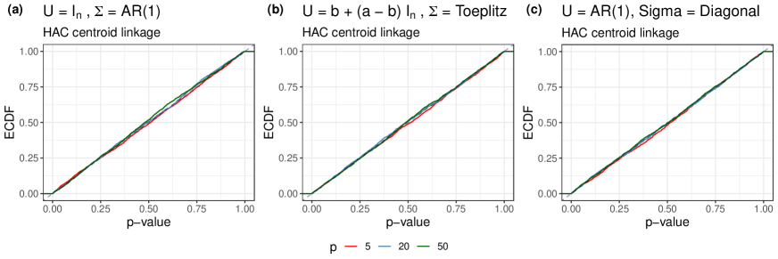
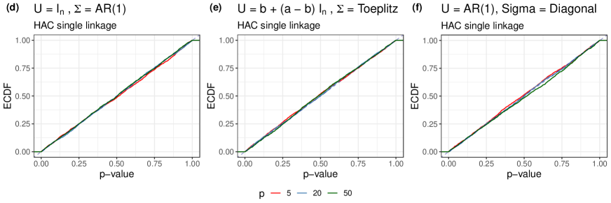
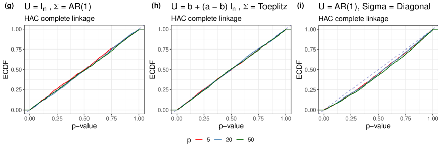
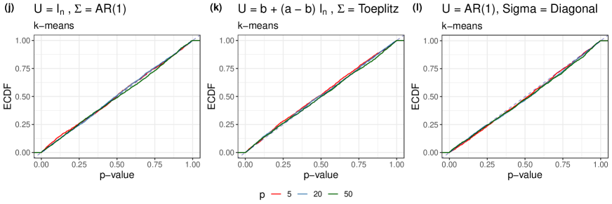
Figure 7: Empirical cumulative distribution functions (ECDF) of $p$-values (2) with $\mathcal{C}$ being a hierarchical agglomerative clustering algorithm (HAC) with centroid (a-c), single (d-f) and complete (g-i) linkage and a $k$-means algorithm (j-l). The ECDF were computed from $M=2000$ realizations of (2) under the three dependence settings $(a)$, $(b)$ and $(c)$ with $\boldsymbol{\mu}=\mathbf{0}_{n\times p}$, $n=100$ and $p\in\{5,20,50\}$.

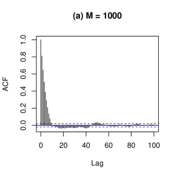
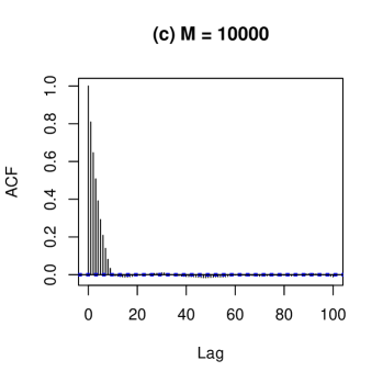
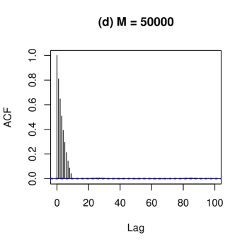
Figure 8: Auto-correlation functions of $M$ concatenated samples of size $n=10$ drawn from an AR(1) process with $\sigma=1$ and $\rho=0.1$, as described in Section D.2.

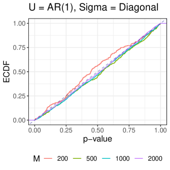
Figure 9: Empirical cumulative distribution functions (ECDF) of $p$-values (2) computed from $M$ iterations of hierarchical clustering with average linkage in the conditions described in Section D.2.

Super-uniform $p$-values for unknown $\mathbf{\Sigma}$

Figure 10 is the counterpart of Figure 3 for $k$-means and HAC with centroid, single and complete linkage. As mentioned in Section 5.2, the obtained $p$-values (2) are stochastically larger than a uniform random variable in all cases. Note that the empirical distribution for HAC with complete linkage and dependence setting $(c)$ (panel (i) in Figure 7) shows a more severe separation from the diagonal. This is explained due to the noise effect discussed in Section D.2. Regarding the simulation for $k$-means clustering, a larger sample size was needed to illustrate a super-uniform null distribution. We set $n=1000$ and $\delta=\{10,12\}$ in that case. For computational speeding-up we chose $p=2$.

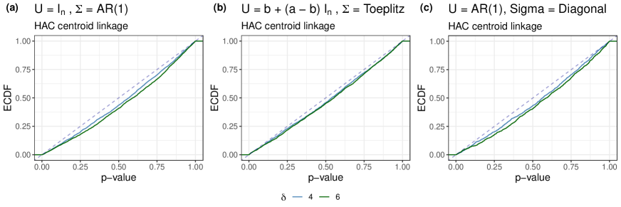
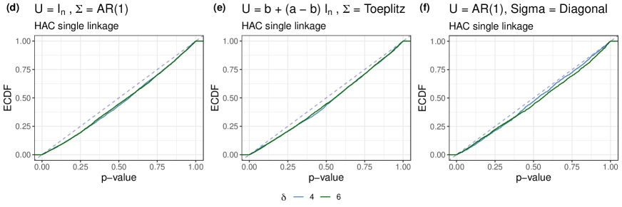
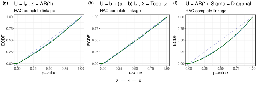
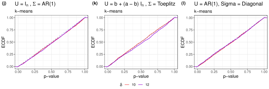
Figure 10: Empirical cumulative distribution functions (ECDF) of $p$-values (2) with $\mathcal{C}$ being a hierarchical clustering algorithm with average linkage. The ECDF were computed from $M=5000$ realizations of (2) under the three dependence settings $(a)$, $(b)$ and $(c)$ with $n=500$, $p=10$ and $\boldsymbol{\mu}$ given by (50) with $\delta\in\{4,6\}$. Only samples for which the null hypothesis held were kept, as described in Section 5.2.

References

- [1] M. Allaoui, M. L. Kherfi, and A. Cheriet. Considerably improving clustering algorithms using UMAP dimensionality reduction technique: A comparative study. In Lecture Notes in Computer Science, pages 317–325. Springer International Publishing, 2020.
- [2] M. P. Allen and D. J. Tildesley. Computer Simulation of Liquids. Oxford University Press, 06 2017.
- [3] R. Appadurai, J. K. Koneru, M. Bonomi, P. Robustelli, and A. Srivastava. Clustering heterogeneous conformational ensembles of intrinsically disordered proteins with t-distributed stochastic neighbor embedding. Journal of Chemical Theory and Computation, June 2023.
- [4] M. S. Bartlett. An Inverse Matrix Adjustment Arising in Discriminant Analysis. The Annals of Mathematical Statistics, 22(1):107 – 111, 1951.
- [5] E. Becht, L. McInnes, J. Healy, C.-A. Dutertre, I. W. H. Kwok, L. G. Ng, F. Ginhoux, and E. W. Newell. Dimensionality reduction for visualizing single-cell data using UMAP. Nature Biotechnology, 37(1):38–44, Dec. 2018.
- [6] P. Bernadó, L. Blanchard, P. Timmins, D. Marion, R. W. H. Ruigrok, and M. Blackledge. A structural model for unfolded proteins from residual dipolar couplings and small-angle x-ray scattering. Proceedings of the National Academy of Sciences of the United States of America, 102(47):17002–17007, 2005.
- [7] A. R. Camacho-Zarco, S. Kalayil, D. Maurin, N. Salvi, E. Delaforge, S. Milles, M. R. Jensen, D. J. Hart, S. Cusack, and M. Blackledge. Molecular basis of host-adaptation interactions between influenza virus polymerase PB2 subunit and ANP32a. Nature Communications, 11(1), July 2020.
- [8] Y. Chen, S. Jewell, and D. Witten. More powerful selective inference for the graph fused lasso. Journal of Computational and Graphical Statistics, 32(2):577–587, 2023.
- [9] Y. T. Chen and D. M. Witten. Selective inference for k-means clustering. Journal of Machine Learning Research, 24(152):1–41, 2023.
- [10] A. Conev, M. M. Rigo, D. Devaurs, A. F. Fonseca, H. Kalavadwala, M. V. de Freitas, C. Clementi, G. Zanatta, D. A. Antunes, and L. E. Kavraki. EnGens: a computational framework for generation and analysis of representative protein conformational ensembles. Briefings in Bioinformatics, 24(4):bbad242, 07 2023.
- [11] A. Diaz-Papkovich, S. Zabad, C. Ben-Eghan, L. Anderson-Trocmé, G. Femerling, V. Nathan, J. Patel, and S. Gravel. Topological stratification of continuous genetic variation in large biobanks, July 2023. bioRxiv 2023.07.06.548007.
- [12] M. W. Dorrity, L. M. Saunders, C. Queitsch, S. Fields, and C. Trapnell. Dimensionality reduction by UMAP to visualize physical and genetic interactions. Nature Communications, 11(1), Mar. 2020.
- [13] P. Dutilleul. The MLE algorithm for the matrix normal distribution. Journal of Statistical Computation and Simulation, 64(2):105–123, 1999.
- [14] H. J. Dyson and P. E. Wright. Intrinsically unstructured proteins and their functions. Nature Reviews Molecular Cell Biology, 6:197–208, 2005.
- [15] W. Fithian, D. Sun, and J. Taylor. Optimal inference after model selection, 2017. arXiv:1410.2597.
- [16] L. L. Gao, J. Bien, and D. Witten. Selective inference for hierarchical clustering. Journal of the American Statistical Association, 0(0):1–11, 2022.
- [17] B. Hivert, D. Agniel, R. Thiébaut, and B. P. Hejblum. Post-clustering difference testing: valid inference and practical considerations, 2022. arXiv:2210.13172.
- [18] S. Holm. A simple sequentially rejective multiple test procedure. Scandinavian Journal of Statistics, 6(2):65–70, 1979.
- [19] R. Horn and C. Johnson. Matrix Analysis. Matrix Analysis. Cambridge University Press, 2013.
- [20] S. Jewell, P. Fearnhead, and D. Witten. Testing for a change in mean after changepoint detection. Journal of the Royal Statistical Society Series B: Statistical Methodology, 84(4):1082–1104, Apr. 2022.
- [21] A. Kessel and N. Ben-Tal. Introduction to Proteins. Chapman and Hall/CRC, Mar. 2018.
- [22] T. Lazar, M. Guharoy, W. Vranken, S. Rauscher, S. J. Wodak, and P. Tompa. Distance-based metrics for comparing conformational ensembles of intrinsically disordered proteins. Biophysical Journal, 118(12):2952–2965, 2020.
- [23] J. Leiner, B. Duan, L. Wasserman, and A. Ramdas. Data fission: splitting a single data point, 2021. arXiv:2112.11079.
- [24] A. Liljas, L. Liljas, J. Piskur, G. Lindblom, P. Nissen, and M. Kjeldgaard. Textbook Of Structural Biology. World Scientific Publishing, Singapore, 2009.
- [25] K. Liu, J. Markovic, and R. Tibshirani. More powerful post-selection inference, with application to the lasso, 2018. arXiv:1801.09037.
- [26] P. Mahalanobis. On the generalized distance in statistics. Proceedings of the National Academy of Sciences, India (Calcutta), (2):44–55, 1936.
- [27] L. McInnes, J. Healy, N. Saul, and L. Großberger. Umap: Uniform manifold approximation and projection. Journal of Open Source Software, 3(29):861, 2018.
- [28] K. Nishikawa, T. Ooi, Y. Isogai, and N. Saitô. Tertiary structure of proteins. i. representation and computation of the conformations. Journal of the Physical Society of Japan, 32(5):1331–1337, 1972.
- [29] V. Ntranos, L. Yi, P. Melsted, and L. Pachter. A discriminative learning approach to differential expression analysis for single-cell RNA-seq. Nature Methods, 16(2):163–166, Jan. 2019.
- [30] C. J. Oldfield and A. K. Dunker. Intrinsically disordered proteins and intrinsically disordered protein regions. Annual Review of Biochemistry, 83(1):553–584, 2014.
- [31] V. Ozenne, F. Bauer, L. Salmon, J.-r. Huang, M. R. Jensen, S. Segard, P. Bernadó, C. Charavay, and M. Blackledge. Flexible-meccano: a tool for the generation of explicit ensemble descriptions of intrinsically disordered proteins and their associated experimental observables. Bioinformatics, 28(11):1463–1470, 2012.
- [32] R. Pearce and Y. Zhang. Deep learning techniques have significantly impacted protein structure prediction and protein design. Current Opinion in Structural Biology, 68:194–207, June 2021.
- [33] D. Phillips. British biochemistry, past and present. In London Biochemical Society Symposia, page 11. Academic Press, 1970.
- [34] D. G. Rasines and G. A. Young. Splitting strategies for post-selection inference. Biometrika, 12 2022. asac070.
- [35] A. Sagar, C. M. Jeffries, M. V. Petoukhov, D. I. Svergun, and P. Bernadó. Comment on the optimal parameters to derive intrinsically disordered protein conformational ensembles from small-angle X-ray scattering data using the ensemble optimization method. Journal of Chemical Theory and Computation, 17(4):2014–2021, 2021.
- [36] J. Shao, S. W. Tanner, N. Thompson, and T. E. Cheatham. Clustering molecular dynamics trajectories: 1. characterizing the performance of different clustering algorithms. Journal of Chemical Theory and Computation, 3(6):2312–2334, Oct. 2007.
- [37] W. F. Trench. Asymptotic distribution of the spectra of a class of generalized kac–murdock–szegö matrices. Linear Algebra and its Applications, 294(1):181–192, 1999.
- [38] L. van der Maaten and G. Hinton. Visualizing data using t-SNE. Journal of Machine Learning Research, 9(86):2579–2605, 2008.
- [39] A. Vandenbon and D. Diez. A clustering-independent method for finding differentially expressed genes in single-cell transcriptome data. Nature Communications, 11(1), Aug. 2020.
- [40] A. P. Verbyla. A note on the inverse covariance matrix of the autoregressive process1. Australian Journal of Statistics, 27(2):221–224, 1985.
- [41] J. Wise. The autocorrelation function and the spectral density function. Biometrika, 42(1/2):151–159, 1955.
- [42] J. Yeh. Real Analysis. World Scientific, 3rd edition, 2014.